On Rendering Synthetic Images for Training an Object Detector

Abstract

We propose a novel approach to synthesizing images that are effective for training object detectors. Starting from a small set of real images, our algorithm estimates the rendering parameters required to synthesize similar images given a coarse 3D model of the target object. These parameters can then be reused to generate an unlimited line of training images of the object of interest in arbitrary 3D poses, which can then be used to increase classification performances.

A key insight of our approach is that the synthetically generated images should be similar to real images, not in terms of image quality, but rather in terms of features used during the detector training. We show in the context of drone, plane, and car detection that using such synthetically generated images yields significantly better performances than simply perturbing real images or even synthesizing images in such way that they look very realistic, as is often done when only limited amounts of training data are available.

url]http://cvlab.epfl.ch/ rozantse, Phone: +41(0)78 9472721 url]http://www.icg.tugraz.at/Members/lepetit url]http://cvlab.epfl.ch/ fua

1 Introduction

It is now widely accepted that when enough training data is available, statistical approaches can address image classification problems [1] very effectively. In the commercial world, this is a key ingredient of high performing face detection software deployed by companies such as Apple and Google. However, there are real-world scenarios in which the required training data is hard to obtain in sufficiently large quantities. For example, our work is motivated by the emerging need for Unmanned Aerial Vehicles (UAVs), or drones, to see and avoid each other as they become increasingly numerous and autonomous in the sky. In this application, training videos are rare and do not cover the full range of possible shapes, poses, and lighting conditions under which they can be seen.

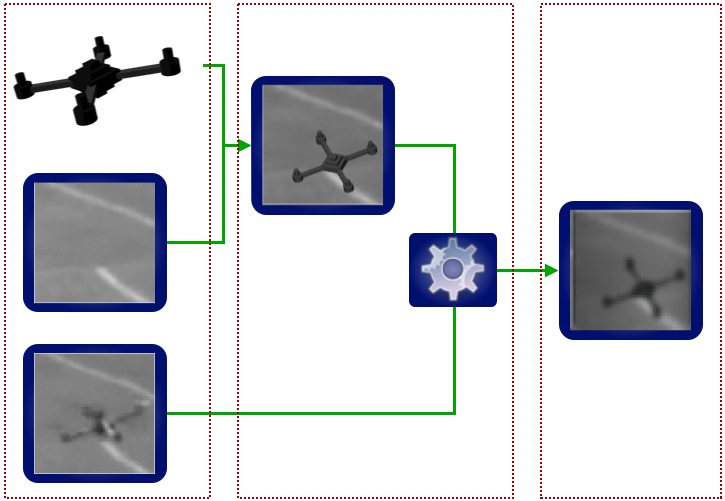
(a) $\qquad\qquad\verb" "$ (b) $\qquad\qquad\verb" "$ (c)

Figure 1: Synthetic data generation pipeline. (a) Input to the system includes a simple model of the object of interest, an image of this object and a background image (it should be the same background as the image of the object has). (b) Overlaying the model on the background yields a synthetic image. This image is then processed to maximize its similarity to a real image from the perspective of the detector. (c) The resulting synthetic image can be used for training the detector.

Our goal therefore is to supplement a small number of available real training samples with an arbitrary large dataset of synthetic ones to improve the detection accuracy of a final classifier. Using synthetic data has been spectacularly successful for 3D body pose estimation with a depth camera [2]. However, depth data do not vary with lighting, motion blur, and other artifacts that affect images from a regular camera, and are therefore comparatively simpler to synthesize.

A training set can also be augmented by applying small deformations and adding noise to the images it contains [3, 4]. This was done for character [5, 6], face [7], and image patch recognition [8]. Such augmentations are typically necessary for the now popular Convolutional Neural Networks [9], which require large amounts of training data.

However, this approach assumes that the original training set is already diverse enough, as the range of synthetic images that can be produced is limited. Moreover simple perturbations are often not enough and special car should be taken. More sophisticated approaches have also been proposed for human detection and pose estimation purposes in [10, 11], but [10] does not model image-acquisition artifacts while [11] involves considerable amounts of manual interaction, which is less desirable. It was recently shown [12] that it is possible to use a 3D car model to first extract appearance information from real images of cars, and use this information to synthesize novel views. Using these images for training purposes improves performance but this approach does not account for other artifacts such as motion blur and is only applicable to objects with relatively simple geometry.

Furthermore, to the best of our knowledge none of these approaches offers a principled way to choose the image synthesis parameters to match the behavior of real-world cameras in the presence of noise. The relevant parameters are typically tuned by hand, which quickly becomes unmanageable when the rendering pipeline is complex. To overcome this limitation, we therefore introduce a fully automated and generic method to estimate these parameters from a small set of available real images to maximize the performance of a detector trained using the resulting synthetic images.

To this end, we start from a small set of real seed images containing a target object and corresponding background images without it, such as the ones depicted by Fig. 1(a). Given a very coarse 3D model of the object of interest, such as that of the drone of Fig. 1(a), we estimate the 3D pose of the object, overlaid onto the background image, and then post-process the resulting composite image so that it is as similar as possible to the real one. This is achieved by automated selection of the post-processing parameters to maximize a similarity between the two images. Once these parameters are found, we can then change the position and the orientation of the object in the images to generate arbitrary large synthetic datasets with realistic imaging artifacts.

A key ingredient of our approach is the similarity function used to measure the difference between real and composite images. An obvious candidate would be the pixel-wise Euclidean distance. However, our goal is not to generate eye-pleasant images, but rather training data that is effective for our intended purpose. We will therefore show that the best similarity depends on the target detection method. We demonstrate this for three widely used methods that are representative of the state-of-the-art: The Deformable Part Model (DPM) method [13], an AdaBoost-based detector [14], and a detector based on Convolutional Neural Networks (CNN) [9]. Together, these methods cover the state-of-the-art in both object detection and image features.

In short, our contribution is a novel and fully automated approach to generating synthetic training image databases that increases detection performance and outperforms the state-of-the-art techniques discussed above, irrespective of the specific detector used. We will demonstrate this in the context of drone, plane, and car detection.

In the remainder of this paper, we first discuss the effects we want to model in our synthetic images. We then describe and compare the different similarity functions to quantify the similarity between synthetic and real images. Furthermore, we demonstrate the power of our approach on aircrafts of very different shapes and flying in various environments and lighting conditions. Finally, we compare our approach to recent work [12] on the Pascal VOC dataset.

2 Related Work

Given the prevalence of Machine Learning based algorithms, capturing and annotating training images has become a major issue, and sometimes a severe bottleneck when such images are hard to acquire. In such cases, using Computer Graphics techniques to generate them is a very attractive alternative.

For example, Optical Character Recognition systems have long been trained using samples created by applying various deformations and adding image noise to actual samples [5, 6]. Similarly, synthetically generated image patches have been successfully used in [15, 16]. Note, however, that neither characters nor patches exhibit the full complexity of natural images and are therefore easier to synthesize. In [2], this approach was used on complete depth images generated from 3D models of people to train classifiers to recover human 3D pose from the output of a Kinect camera. This has been remarkably successful, in large part because it provides a way to create arbitrarily large training dataset. However, depth images also lack many of the imaging artefacts present in ordinary images, such as motion blur or lighting effects, which make it difficult to use such an approach for video imagery.

This was attempted in [10] by generating images of pedestrians in various poses and environments to train a pedestrian detector. The results are encouraging but the method does not take complex imaging artefacts into account. More recently, an approach to creating more realistic synthetic images by extracting people’s silhouettes from real images, and superimposing them over various backgrounds was proposed [11]. However, it is very specific to pedestrian detection and requires a considerable amount of manual annotation.

Like ours, the approach of [12] relies on both real training images and a 3D model. After registering the 3D model to the images, the material and lighting properties of the different object components are estimated and used to synthesise new views of the 3D model. However, it does not take into account other artifacts such as motion blur and requires precise registration.

Of course, generic image synthesis techniques have also been used in computer vision for many other purposes, such as optimizing camera tracking algorithms [17], evaluation of algorithms [18, 19, 20, 21, 22, 23], gesture recognition and pose estimation [24, 25], or rendering virtual objects that merge well with real images [26]. Some of these approaches simply project the 3D model of the object of interest on an arbitrary background image. Others add post-processing on similarly generated synthetic images in order to make them look realistic. However, to the best of our knowledge none of them estimate neither how realistic the resulting images are, nor how suitable they are for the application itself.

In this work, we will use some of the same approaches to synthesizing realistic images. This being said, visual realism is not our end goal, but rather the classification performance improvement. As such our algorithm, unlike the others, automatically optimizes the rendering parameters solely for this purpose.

3 Generating Synthetic Images

As illustrated by Fig. 1, while our pipeline is simple, it depends on many parameters that would be hard to choose by hand. We use simple CAD models, such as that of Fig. 1(a), which roughly captures the target object geometry. We assume that we are given a small set of real images featuring the target object and a corresponding set of background images without it. As we will explain, these background images can usually be extracted from the training video sequence itself. In cases where the background is not visible at any time, it is still possible to estimate it by cutting out the object from the original images and using a texture filling algorithm. This approach will be more thoroughly discussed in Section 5.3.

For each real image, we then compute 5 pose parameters, that include 3 orientations $(\alpha^{p},\beta^{p},\gamma^{p})$ and 2 translations $(t^{p}_{x},t^{p}_{y})$, which lets us project the 3D model at the desired location. Note that as we use multi-scale detector, we do not need to vary the scale of the object.

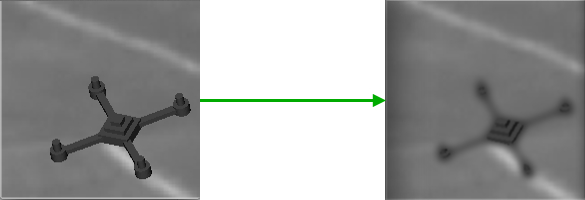
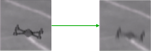
(a) Boundaries blurring		(b) Motion blurring
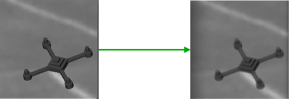
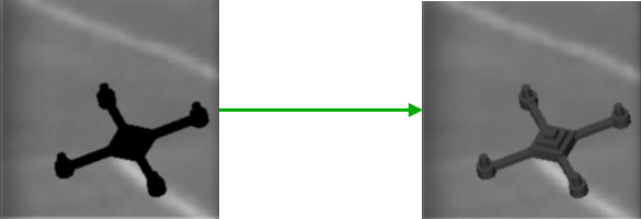
(c) Random noise		(d) Diffuse coefficient of material variation

Figure 2: The four post-processing effects we use for increasing the similarity between the real and synthetic images.

As shown in Fig. 2, we then post-process the synthetic image to maximize its similarity to the real image. This involves:

• Object boundary blurring (BB). The discrete nature of the image sensor causes a mixture of the intensities of the background and the target object along its boundaries. To simulate this effect we apply Gaussian blurring along the object boundaries after the object image has been overlaid on the background image. This is controlled by the standard deviation $\sigma^{s}$ of the Gaussian kernel used for smoothing.

• Motion blurring (MB). This mimics the blurring effect that affects on fast moving objects if the shutter time of the camera is too long. To simulate this effect we use anisotropic Gaussian blurring applied to the pixels of the object in the direction of its motion. The parameters are the two standard deviations $\sigma^{m}_{u}$ and $\sigma^{m}_{v}$ of the Gaussian kernel and the angle $\alpha^{m}$ of the motion.

• Random noise (RN). This emulates the shot noise added to the image by the camera. To simulate this effect we simply add independent Gaussian noise to the pixel intensities. Note this is limited to the image pixels that correspond to the inserted object, as the background images are real ones and already contain similar noise. This is controlled by the standard deviation $\sigma^{n}$ of the Gaussian distribution used to generate the noise.

• Material properties (MP). We also vary the material properties, by changing the weight $w^{d}$ of the diffuse reflection. This allows us not only to vary the color of the object, but also to introduce some diffuse lighting effects. While we do not take specularities into account, this would be a very natural extension to our approach.

We refer to these synthetic data generation parameters as capture parameters

$$\Theta=[\underbrace{\alpha^{p},\beta^{p},\gamma^{p},t^{p}_{x},t^{p}_{y}}_{\text{pose}},\underbrace{\sigma^{s},\sigma^{m}_{u},\sigma^{m}_{v},\alpha^{m},\sigma^{n},w^{d}}_{\text{capture}}]^{\top}\>.$$ (1)

These parameters are challenging to tune because they are heavily correlated. This is particularly true of object pose and direction of motion blur, as well of boundary blurring and motion blurring. Thus our goal is to estimate the $\Theta$ parameters for every seed real image that we use for synthetic data generation. Given the background images and the corresponding $\Theta$ parameters, we retain the capture parameters and randomize the pose ones to generate arbitrary large numbers of synthetic images that will be realistic enough to be used for training the object detector. We explain below how we recover these $\Theta$ parameters.

4 Optimizing the Rendering Parameters

To optimize the pose and capture parameters in $\Theta$, we rely on a small set of real images of the target object, together with the corresponding images of the background without the target.

Starting from a background image on which we render the CAD model of the target object, we optimize the rendering parameters to reproduce the corresponding real image. This optimization is performed on each image independently, because the same capture parameters do not necessarily apply to all of them. More formally, we consider the set of pairs of real images $\{(X_{i},B_{i})\}^{N}_{i=0}$, where $X_{i}\in$ $\chi$ is the $i^{\text{th}}$ image of the object and $B_{i}\in$ $\chi$ is the background image for $X_{i}$. Let $d:$$\chi$ $\times$ $\chi$ $\rightarrow\mathbf{R}^{+}$ be a similarity function, which we use to compare two images, and which we will define explicitly in Sect. 4.1. Lastly, let $S(\Theta,B_{i})\in$ $\chi$ represent the synthetically rendered image by applying the synthetic data generation process with parameters $\Theta$ to the Background $B_{i}$

To find the set of parameters $\Theta$ that best corresponds to real image $X_{i}$, we look for

$$\Theta^{(i)}=\operatorname*{\text{argmin}}_{\Theta}d(X_{i},S(\Theta,B_{i}))$$ (2)

by Simulated Annealing [27]. This approach is widely used for solving non-continuous optimization problems with a large number of parameters. In practice, we initialize the pose parameters by manually providing the object center, which could be avoided with a more sophisticated optimization algorithm. Capture parameters are initialized randomly. This optimization takes a few seconds on each of our $40\times 40$ images.

The capture parameters in $\Theta$ depend on viewing conditions, such as lighting and weather conditions, which is why we perform the optimization in each image independently. Fig. 3 describes their distributions across images. Note that these distributions are absolutely not Gaussian and that it would therefore be non-trivial to describe them analytically.

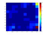
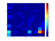
$\sigma^{n}$		$\sigma^{n}$		$\sigma^{m}_{u}$
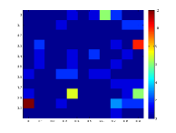
	$\sigma^{m}_{v}$		$\sigma^{s}$		$\sigma^{m}_{v}$

Figure 3: Each histogram depicts the joint distribution of different pairs of capture parameters. (best seen in color)

4.1 Image Similarity Measures

The resulting parameters depend critically on the similarity function $d(\cdot,\cdot)$ used to evaluate how close the two images are to each other. The simplest is the Euclidean distance between the intensity values of corresponding pixels

$$d_{\text{Eucl}}(X_{\text{re}},X_{\text{sy}})=\sqrt{\mathop{\Sigma}\limits_{v=1}^{H}\mathop{\Sigma}\limits_{u=1}^{W}\big{(}X_{\text{re}}(u,v)-X_{\text{sy}}(u,v)\big{)}^{2}}\>,$$ (3)

where $X_{\text{re}}$ and $X_{\text{sy}}$ are the real and synthetic images respectively, and $W$ and $H$ denote the images dimensions.

However, since our goal is to generate synthetic images that are more effective to train a detection method, we will see this is not the best possible choice, for our purposes.

More specifically, we evaluated our approach in conjunction with three commonly used object detectors—DPM [13], an AdaBoost-based detector [14], and a CNN [9]—and we therefore introduce three different similarity functions, each one based on the image features used by one of these methods. We will show that our approach to image generation works best when relying on the distance function corresponding to the detection method.

Since DPM relies on Histograms-of-Gradients (HoG) [28], the first similarity function we consider the distance between the HoG vectors [28] computed for the two images as the similarity function

$$d_{\text{HoG}}(X_{\text{re}},X_{\text{sy}})=\sqrt{\mathop{\Sigma}\limits_{i=1}^{L}\big{(}\text{HoG}_{i}(X_{\text{re}})-\text{HoG}_{i}(X_{\text{sy}})\big{)}^{2}}\>,$$ (4)

where $\text{HoG}_{i}(X)$ is the $i^{\text{th}}$ coordinate of the HoG vector computed for image $X$.

We also consider an AdaBoost detector, whose weak learners rely on the image gradients proposed in [29]. We write

$$h_{R,o,\tau}(X)=\left\{\begin{array}[]{ll}1,&\text{ if }E(X,R,o)>\tau,\\ 0,&\text{ otherwise.}\\ \end{array}\right.$$ (5)

These weak learners are parametrized by a region $R$, an orientation $o$, and a threshold $\tau$. $E(X,R,e)$ is the normalized image gradient energy over region $R$ in $X$ and in orientation $o$. We therefore introduce the additional function:

$$d_{\text{WL}}^{H}(X_{\text{re}},X_{\text{sy}})=\sqrt{\mathop{\Sigma}\limits_{i=1}\limits^{L}\alpha_{i}\big{(}h_{i}(X_{\text{re}})-h_{i}(X_{\text{sy}})\big{)}^{2}}\>,$$ (6)

where $L$ is the number of weak learners $h_{i}$ with their corresponding weights $\alpha_{i}$. We tried two different methods to build such a set:

• $d_{\text{WL}}^{R}(X_{\text{re}},X_{\text{sy}})$ will denote the previous similarity function when random weak learners, each with a weight $\alpha=1$, are used;

• $d_{\text{WL}}^{L}(X_{\text{re}},X_{\text{sy}})$ will denote the previous similarity function when a set of weak learners and their weights selected by AdaBoost on the seed real images is used.

The third detection method we consider is a Convolutional Neural Network (CNN) which, unlike the previous two, does not rely on hard-coded image features but learns them instead. We therefore first train a CNN on the real seed images only and consider the distance

$$d_{\text{CNN}}(X_{\text{re}},X_{\text{sy}})=\sqrt{\mathop{\Sigma}\limits_{n=2}^{N}\mathop{\Sigma}\limits_{i=1}^{L_{n}}\big{(}\text{CNN}^{n}_{i}(X_{\text{re}})-\text{CNN}^{n}_{i}(X_{\text{sy}})\big{)}^{2}}\>,$$ (7)

where $\text{CNN}^{n}_{i}(X)$ is the value of the $i^{\text{th}}$ neuron of the $n^{\text{th}}$ layer of the Convolutional Neural Network; $N$ is the number of layers in the CNN; $L_{n}$ is the number of neurons of the $n^{\text{th}}$ layer of CNN.

In Fig. 4, we show synthetic images with the corresponding real seed images. Each image was obtained by finding the rendering parameters that minimize one of the five similarity functions introduced above.

Original		$d_{\text{Eucl}}$	$d_{\text{HoG}}$	$d_{\text{WL}}^{R}$	$d_{\text{WL}}^{L}$	$d_{\text{CNN}}$

Figure 4: Samples of real images with corresponding synthetic ones. The $\Theta$ parameters for the synthetic images were optimised using different image similarity functions.

Training Data
Evaluation Data

Figure 5: Sample real images both for training and evaluation from the UAV dataset. The evaluation images, while created using a single UAV, are very challenging as they are low-resolution while exhibiting significant lighting, background, and pose variations.

5 Results

In this section, we first introduce the three datasets that we used for training and testing of our algorithms. Then we compare our synthetic data generation approach with several baselines, and evaluate the importance of each of our rendering effects. Our next step is to show the significance of the optimization of the $\Theta$ rendering parameters. Further on we experimentally estimate the optimal ratio between synthetic and real samples used for training. We then show that our algorithm is able to generalize to multiple kinds of aircrafts. Finally we compare our approach to a very recent one on realistic data generation on the PASCAL VOC dataset.

• UAV Dataset. This dataset contains challenging images that were acquired from the camera of a flying UAV. In these low-resolution images one can see another drone that flies around and appears against different backgrounds and under various lighting conditions. Even though only one drone was used to produce the images, the dataset includes many of the challenges that outdoor environments pose, such as large illumination and background changes. We use it to investigate the impact of the different effects our rendering pipeline includes.

• Aircraft dataset. This dataset contains images of different planes seen against changing backgrounds and under a variety of weather and lighting conditions. We use it to demonstrate that our approach generalizes to a much larger class of objects than simply drones. As in the case of the UAV dataset, we will demonstrate that regardless of the machine learning method used to detect the target objects, we can improve performance by appropriately generating our synthetic images.

• PASCAL VOC 2007. We use this well-known Computer Vision benchmark to compare our approach to a very recent work on synthetic view generation [12]. As in [12], we restrict ourselves here to the car class, which nevertheless further demonstrates the versatility of our approach.

We will present our results in terms of both recall $r$ vs precision $p$ curves and average precision AveP, defined as $\int\limits^{1}\limits_{0}p(r)dr$. Some additional results and video sequences can be found on the webpage of the project.

5.1 Gauging the Various Components of the Approach using the UAV Dataset

We created a dataset of 2,000 images of UAVs in various environments and seen under different lighting conditions. Fig. 5 depicts some of the images. The images were captured by one UAV filming another one while they were both flying.

Fig. 6 depicts detections by an AdaBoost classifier trained using either real images only or both real and synthetic images. We will quantify the observed performance improvement in the remainder of this section. In Fig. 7, we show additional examples of detections by the detector trained on both real and synthetic data as well as some failure cases to illustrate how challenging this dataset is.

We first describe the acquisition process and then use these UAV images to test individual components of our pipeline and to evaluate overall performance.

Real Data
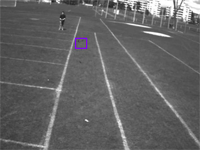
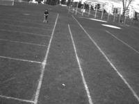
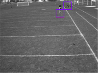
Real+Synth Data
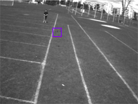
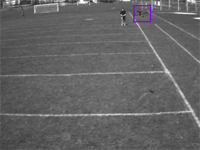
Real Data
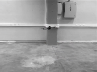
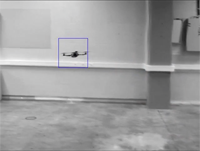
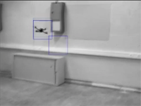
Real+Synth Data

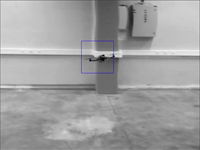
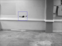
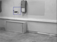
Figure 6: Qualitative comparison of the performance of the detectors trained just on real data versus both real and synthetic data.

Detections
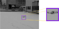
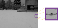
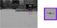
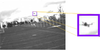
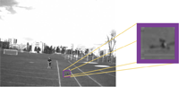
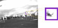
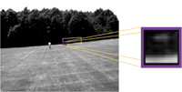
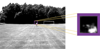
Missed and False Detections

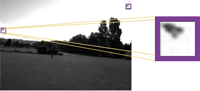
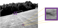
Figure 7: Top rows: More sample detections by the AdaBoost detector trained using both real and synthetic data. Bottom row: Missed or false detections to highlight the challenges that the dataset provides for the detector. (best seen in color)

5.1.1 Experimental Setup

To obtain the background images required to render the composite ones, we first aligned consecutive frames by computing the homographies between the frames, and kept the median intensity at each location of the aligned images.

The training and testing videos were acquired in different environments and feature different backgrounds. The CAD model of the UAV used for rendering only coarsely outlines the main geometrical structure of the real object, as illustrated by Fig. 1(a). Negative training and testing samples were obtained by randomly sampling the backgrounds of the training images. For detection, we use a sliding window approach that applies the detector at every spatial location and at different scales of the whole image. Non-maximum suppression is then applied to the response image scale-space.

The detection methods in the experiments are trained with a combination of real and synthetic data and tested on the real data only.

5.1.2 Comparing against simply Perturbing the Real Images

A broadly used approach to augmenting a training set is to perturb the available images using simple image transformations [5, 6]. Table 1 compares the performances of all three selected detectors when being trained on images generated either in this way or using our approach. The perturbations involve combining rotation, translation, mirroring, blurring and adding noise to the original images.

Our approach significantly outperforms this simple technique. This can be explained by the fact that we generate realistic combinations of 3D poses and background that are not present in the seed images.

		Using real	By perturbing	Our method
		images only	the real images
Detection method:		Average precision:
DPM		0.84	0.87	0.93
AdaBoost		0.80	0.83	0.92
CNN		0.85	0.86	0.89

Table 1: Comparing average precisions for each detection method when either perturbing real training images or using our approach with the optimal number of synthetic images and the appropriate distance measure . Our approach significantly outperforms this traditional method.

5.1.3 Relative Importance of the Various Rendering Effects

To demonstrate that correctly setting each one of the capture parameters introduced in Section 3 truly matters, we performed the following set of experiments. For each effect—object boundary blurring, Motion blurring, Random noise, Material properties—we set the corresponding value in the capture parameters $\Theta$ of Eq. 1 to 0 to suppress its influence and optimized the other parameters using the appropriate similarity measure for each detection method. We then used the resulting $\Theta$’s to generate the synthetic images, trained the corresponding detector on these images and evaluated is on the test images. The results are shown in Fig. 8. Correctly modeling each effect clearly has a positive influence on final performance.

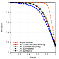
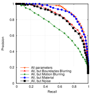
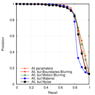
DPM and $d_{\text{HoG}}(.,.)$ AdaBoost and $d_{\text{WL}}^{L}(.,.)$ CNN and $d_{\text{CNN}}(.,.)$

Synthetic data generation effects: All no BB no MB no RN no MP Detection method: Average precision: DPM 0.93 0.83 0.84 0.83 0.80 AdaBoost 0.92 0.85 0.71 0.75 0.91 CNN 0.89 0.88 0.89 0.88 0.85

Figure 8: Evaluating the importance of each capture parameter. Each one clearly has a positive influence of the quality of the synthetic data. However, their respective impacts depends on the specific detection method. (best seen in color)

5.1.4 Importance of Optimizing over the Rendering Parameters

To show the importance of optimizing over the capture parameters $\Theta$, we compare in Fig. 9 the final performance obtained using optimized parameters with the final performance obtained with random parameters drawn from a uniform distribution. The minimum and maximum values of the uniform distribution were taken as the minimum and maximum values of the optimized parameters. Our optimization-based approach clearly brings a significant improvement.

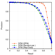
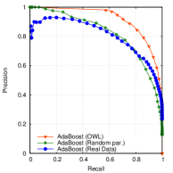
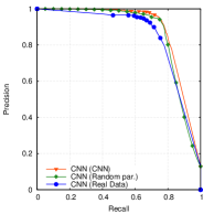
DPM AdaBoost CNN

Using real Random Optimized images only parameters parameters Classification method: Average precision: DPM 0.84 0.82 0.93 AdaBoost 0.80 0.82 0.92 CNN 0.85 0.87 0.89

Figure 9: Comparison of the performances of different detectors trained on real and synthetic data generated using corresponding similarity measures with those where the capture parameters are randomly selected. The optimized parameters always yield better performance. (best seen in color)

5.1.5 Influence of the Number of Synthetic and Real Images

To evaluate how much we can improve the performances using synthetic images generated with our approach, we trained each of the detection methods we consider with different numbers of synthetic samples in addition to the real training samples. For each detector, the synthetic samples were generated using the parameters obtained using the appropriate similarity functions.

Fig. 10 compares the performances of these detectors when varying the number of synthetic samples. It can be seen that using the synthetic images significantly improves performance over using the real images alone. However, this is only true up to a point. When there are too many synthetic images, the performance eventually decreases because the influence of the real images gets drowned out. In practice, this means that for best performance, it makes sense to use a validation set to ascertain the optimal ratio of synthetic to real images.

From these experiments we can conclude that the best ratio of synthetic and real examples that should be used for training depends on the detection algorithm. AdaBoost achieves its highest accuracy with $100$ synthetic images for each real one, DPM with 50 synthetic images for each real one, and CNN with $15-20$ synthetic images for each real one.

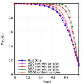
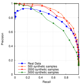
DPM and $d_{\text{HoG}}(.,.)$	AdaBoost and $d_{\text{WL}}^{R}(.,.)$
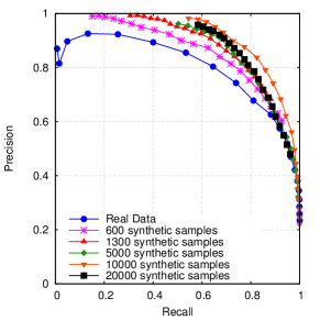
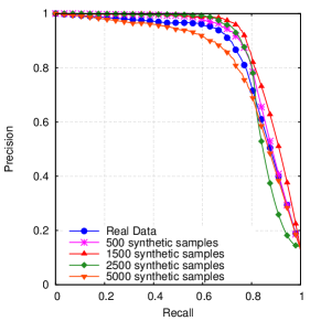
AdaBoost and $d_{\text{WL}}^{L}(.,.)$	CNN and $d_{\text{CNN}}(.,.)$

Figure 10: We varied the number of synthetic images used for training, for three detection methods, using their corresponding similarity measures. Using both real and synthetic data for training phase increases performances compared to real data used alone. However using too much synthetic data may also hurt. (best seen in color)

We also evaluated the influence of the number of seed real images on the final performances, by decreasing the number of real images used to optimize the rendering parameters. Fig. 11 shows the results for the AdaBoost detector. Using as few as 12 real samples is enough to generate synthetic samples that allows us to outperform a detector trained with about 8 times as many real images. Unsurprisingly, increasing the number of seed real images results in an improvement of the final performances.

		Similarity measure:
	Using real	$d_{\text{Eucl}}(.,.)$	$d_{\text{HoG}}(.,.)$	$d_{\text{WL}}^{R}(.,.)$	$d_{\text{WL}}^{L}(.,.)$	$d_{\text{CNN}}(.,.)$
	images only
Detection method:	Average precision:
DPM	0.84	0.78	0.93	0.70	0.72	0.67
AdaBoost	0.80	0.72	0.85	0.89	0.92	0.75
CNN	0.85	0.84	0.84	0.84	0.86	0.89

Table 2: Comparison of average precisions for each detection method, when the optimal number of synthetic images is used. Each detection method performs best with the corresponding similarity function.

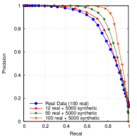
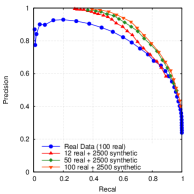
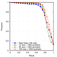
DPM and $d_{\text{HoG}}(.,.)$	AdaBoost and $d_{\text{WL}}^{L}(.,.)$	CNN and $d_{\text{CNN}}(.,.)$

Figure 11: Performance of the DPM, AdaBoost, and CNN detectors for different numbers of seed real images. Using as few as 12 real samples is enough to generate synthetic samples that allow us to outperform a detector trained with 100 images. For each detector, the synthetic images were generated using the corresponding similarity measure.

5.1.6 Optimal Performance

In this section, for each detection method, we use the optimal numbers of synthetic samples as discussed in the previous section. For comparison purposes, we also estimated the optimal numbers of synthetic samples when using the Euclidean distance $d_{\text{Eucl}}(.,.)$ as similarity measure.

Table 2 confirms that each detection method performs best when trained using synthetic images, generated using appropriate similarity measure, as discussed in Section 4.1. In particular, using the Euclidean distance is not only ineffective, but actually yields worse results than not using synthetic images at all. Interestingly, the best performance is obtained with DPM trained with both real and synthetic images, even though CNN was better than DPM when no synthetic images were used.

5.2 Detecting Multiple Kinds of Aircrafts

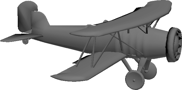
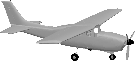
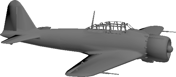
Figure 12: The three CAD models we used for the Aircraft dataset. They are freely available on the internet.

For the Aircraft dataset, we generated synthetic data using CAD models depicted by Fig. 12 of three types of fixed-wing aircrafts and tested them on different real video sequences. We use 100 real images of these three aircraft types along with their corresponding background images. These images were collected by manually annotating different video sequences where the aircrafts fly in different weather conditions and appear at different angles. Sample images from this dataset are shown on Fig. 13.

Figure 13: Sample seed real images from the Aircraft dataset.

Here, we used an AdaBoost detector trained using real and synthetic images generated based on the $d_{\text{WL}}^{L}(.,.)$ similarity function of Section 4.1. We generated 10,000 synthetic samples to supplement the real images and used them as a training dataset. Fig. 14 depicts sample synthetic images.

Figure 14: Generated samples of aircrafts.

The test images come from 8 video sequences, one of which contains 5,000 frames, while the others are made of 500 frames. These sequences show different types of aircrafts flying in different environments and weather conditions. In Table 3 and Fig. 15, we compare results using real images only against an optimal combination of real and synthetic images.

Using the detector trained on both real and synthetic images we achieve about $90\%$ detection accuracy, as opposed to approximately $65\%$ when using real images only. This large improvement can be explained by the fact that we have only 100 real images containing three different models, while we generated 100 images for each real seed image, which results in total in 10,000 positive examples. Table 3 illustrate the best accuracy one can get varying the number of synthetic samples being added to the training set. Sample detections are shown in Fig. 16, which also depicts some failure cases.

		Similarity measure:
	Using real	$d_{\text{Eucl}}(.,.)$	$d_{\text{HoG}}(.,.)$	$d_{\text{WL}}^{R}(.,.)$	$d_{\text{WL}}^{L}(.,.)$	$d_{\text{CNN}}(.,.)$
	images only
Detection method:	Average precision:
DPM	0.79	0.83	0.88	0.85	0.86	0.81
AdaBoost	0.65	0.75	0.84	0.87	0.92	0.73
CNN	0.72	0.75	0.85	0.70	0.83	0.88

Table 3: Comparing average precisions for each detection method when the optimal number of synthetic images is used for the Aircraft dataset. Each detection method performs best when using the corresponding similarity function.

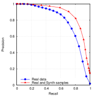
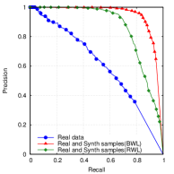
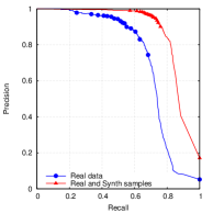
DPM and $d_{\text{HoG}}(.,.)$	AdaBoost and $d_{\text{WL}}^{L,R}(.,.)$	CNN and $d_{\text{CNN}}(.,.)$

Figure 15: Comparing the accuracy of the detectors trained with real images only (blue) against those trained using both synthetic and real images (red or green). AdaBoost in particular does not perform very well with only the real images because 100 samples are not enough to train the algorithm to detect 3 different kinds of aircrafts. Nevertheless, introducing synthetic images lets us enrich the training set to the point where performance improves substantially in all cases. In the AdaBoost case, the red curve is obtained by using the $d_{\text{WL}}^{L}(.,.)$ similarity measure and the green one the $d_{\text{WL}}^{R}(.,.)$ similarity measure.

Detections
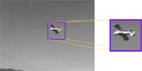
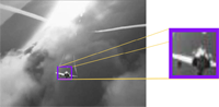
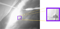
Missed and False Detections

Figure 16: Examples of detections and some errors made by the detector, trained on both real and synthetic samples, and evaluated on the Aircraft dataset.

5.3 Comparing against another recent Image-Based Synthesis Approach

We compare here our approach with the one of [12], which was applied to car detection on the PASCAL VOC car dataset. Like ours, it uses a CAD model of the target object and seed real images. Its main contributions are the estimation of the material properties of every car component in a real image and the exploitation of this information to generate new synthetic views, which are then used to supplement real ones to train a DPM detector. This requires registration of the model so that it precisely fits the car in the image and the image texture can then back-projected onto the car model, so that material properties can be assigned to each visible part of the model. To generate a new view, the model is rotated in 3D and re-projected in the scene, which includes the ground plane and the background plane. This ends up making some previously invisible parts of the car visible. Material properties for these newly visible parts are estimated using a weighted sum of the properties of the parts whose material properties have already been estimated.

Since, our algorithm requires background images in addition to the model and seed real images, we derived them from the seed images by cutting out the car and filling the empty space using content aware texture filling [30]. Sample images are shown in Fig. 17.

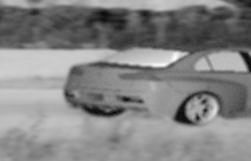
(a)		(b)	(c)

Figure 17: (a) Sample synthetic images of cars generated by our approach. (b, c) Patches extracted from these images emphasizing the importance of the boundary and motion blurring effects.

The images of the Pascal VOC dataset being in color, for a fair comparison against [12] that exploits this fact, we extended our approach to color images by simply optimizing on the $\Theta$ parameters on the three RGB channels independently, which yields three sets of parameters for every image. These parameters are then used to generate separate synthetic images for every channel, and finally combined in one RGB image. We vary the pose of the car model, but also the direction of the light source, which cannot be done with [12]. The results of this combination are presented in Fig. 18. The car in Fig. 18(b) does not look very realistic, because the same properties are applied to all the components of the car. A more sophisticated model would solve this issue, however we already obtain satisfying results using this simplistic rendering, which confirms that producing visually pleasing synthetic images is not a primary requirement. Some detections made by the 5 component DPM framework, trained on both real and synthetic data are presented in the Fig. 19.

Table 4 shows that we outperform [12] even though our approach was originally designed to generate small image patches centered on the target object. Furthermore, as shown in the previous sections, it is applicable to low-resolution images with very limited texture, for which the the method of [12] is not well adapted. Furthermore, if we don’t use color, the performance drops by only 1-2%, which is not very large.

Test set	Training set abcaaaabcabcabcabcabcabcabcabc	Avg. Precision
Number of components:		$N$ = 3	$N$ = 4	$N$ = 5
VOC 2007	Side	16.2	18.4	16.7
	Side+Synth [12]	30.2	31.4	33.2
	Side+Synth (Our method)	35.1	37.9	38.0
	Full	51.7	53.4	50.7
	Full+Synth [12]	50.2	53.1	50.9
	Full+Synth (Our method)	52.1	52.9	55.3

Table 4: Comparing the performances of the DPM detector on the PASCAL VOC car dataset when trained with the method of [12] and our method as a function of $N$, the number of DPM components. The performance of the detectors trained using only the real images is also given for reference.

(a)	(b)	(c)

Figure 18: Sample color synthetic images of cars, generated by our system. (b) does not look very realistic, because the same properties are applied to all the components of the car. A more sophisticated model could be used to address this issue. However realism does not seem to be critical for our purposes since our simplistic model is sufficient to outperform [12].

Correct Detections
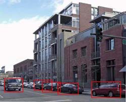
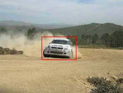
Mis-detections

Figure 19: Sample detections made by the 5 component DPM, trained on the full real VOC dataset, supplemented by synthetic data, generated by our method. Last row shows mis-detections. (best seen in color)

6 Conclusion

We have shown that by properly optimizing the parameters of a very simple rendering pipeline, we can generate synthetic images that significantly improve the performance of an object detector when used for training. We believe our parameter optimization scheme is a powerful tool to manage the large numbers of parameters a more complex rendering pipeline could have. It therefore opens new doors towards the use of sophisticated Computer Graphics and post-processing effects to generate images even closer to real ones, and to relax the cumbersome need for large numbers of real images to train Computer Vision methods.

Artem Rozantsev joined EPFL in 2012 as Ph.D. candidate at CVLab, under the supervision of Prof. Pascal Fua and Prof. Vincent Lepetit. He received his Specialist degree in Mathematics and Computer Science from Lomonosov Moscow State University. His main research interests include object detection, synthetic data generation and machine learning.

Vincent Lepetit is a Professor at the Institute for Computer Graphics and Vision, TU Graz and a Visiting Professor at the Computer Vision Laboratory, EPFL. He received the engineering and master degrees in Computer Science from the ESIAL in 1996. He received the PhD degree in Computer Vision in 2001 from the University of Nancy, France, after working in the ISA INRIA team. He then joined the Virtual Reality Lab at EPFL as a post-doctoral fellow and became a founding member of the Computer Vision Laboratory. His research interests include vision-based Augmented Reality, 3D camera tracking, Machine Learning, object recognition, and 3D reconstruction.

Pascal Fua received an engineering degree from Ecole Polytechnique, Paris, in 1984 and the Ph.D. degree in Computer Science from the University of Orsay in 1989. He joined EPFL in 1996 where he is now a Professor in the School of Computer and Communication Science. Before that, he worked at SRI International and at INRIA Sophia-Antipolis as a Computer Scientist. His research interests include shape modeling and motion recovery from images, analysis of microscopy images, and Augmented Reality. He has (co)authored over 150 publications in refereed journals and conferences. He is an IEEE fellow and has been a PAMI associate editor. He often serves as program committee member, area chair, or program chair of major vision conferences.

References

- [1] Q. Le, M. Ranzato, R. Monga, M. Devin, K. Chen, G. Corrado, J. Dean, A. Ng, Building High-Level Features Using Large Scale Unsupervised Learning, in: International Conference on Machine Learning, 2012.
- [2] J. Shotton, R. Girshick, A. Fitzgibbon, T. Sharp, M. Cook, M. Finocchio, R. Moore, P. Kohli, A. Criminisi, A. Kipman, A. Blake, Efficient Human Pose Estimation from Single Depth Images, IEEE Transactions on Pattern Analysis and Machine Intelligence 99.
- [3] C. Burges, B. Schölkopf, Improving the Accuracy and Speed of Support Vector Machines, in: Advances in Neural Information Processing Systems, 1997, pp. 375–381.
- [4] D. Decoste, B. Schölkopf, Training Invariant Support Vector Machines, Machine Learning 46 (2002) 161–190.
- [5] Y. LeCun, L. Bottou, Y. Bengio, P. Haffner, Gradient-Based Learning Applied to Document Recognition, in: Intelligent Signal Processing, 2001, pp. 306–351.
- [6] T. Varga, H. Bunke, Generation of Synthetic Training Data for an Hmm-Based Handwriting Recognition System, in: 7th Int. Conference on Document Analysis and Recognition, 2003, pp. 618–622.
- [7] F. Fleuret, D. Geman, Coarse-To-Fine Visual Selection, International Journal of Computer Vision 41 (1) (2001) 85–107.
- [8] V. Lepetit, P. Lagger, P. Fua, Randomized Trees for Real-Time Keypoint Recognition, in: Conference on Computer Vision and Pattern Recognition, 2005.
- [9] T. Serre, L. Wolf, S. Bileschi, M. Riesenhuber, T. Poggio, Robust Object Recognition with Cortex-Like Mechanisms, IEEE Transactions on Pattern Analysis and Machine Intelligence.
- [10] J. Marin, D. Vázquez, D. Geronimo, A. M. Lopez, Learning Appearance in Virtual Scenarios for Pedestrian Detection, in: Conference on Computer Vision and Pattern Recognition, 2010, pp. 137–144.
- [11] L. Pishchulin, A. Jain, A. Mykhaylo, T. Thormaehlen, B. Schiele, Articulated People Detection and Pose Estimation: Reshaping the Future, in: Conference on Computer Vision and Pattern Recognition, 2012.
- [12] K. Rematas, T. Ritschel, M. Fritz, T. Tuytelaars, Image-Based Synthesis and Re-Synthesis of Viewpoints Guided by 3D Models, in: Conference on Computer Vision and Pattern Recognition, 2014.
- [13] P. Felzenszwalb, D. Mcallester, D. Ramanan, A Discriminatively Trained, Multiscale, Deformable Part Model, in: Conference on Computer Vision and Pattern Recognition, 2008, pp. 1–8.
- [14] Y. Freund, R. Schapire, A Decision-Theoretic Generalization of On-Line Learning and an Application to Boosting, in: European Conference on Computational Learning Theory, 1995, pp. 23–37.
- [15] V. Lepetit, P. Fua, Keypoint Recognition Using Randomized Trees, IEEE Transactions on Pattern Analysis and Machine Intelligence 28 (9) (2006) 1465–1479.
- [16] D. Cireşan, A. Giusti, L. Gambardella, J. Schmidhuber, Deep Neural Networks Segment Neuronal Membranes in Electron Microscopy Images, in: Advances in Neural Information Processing Systems, 2012.
- [17] A. Handa, R. Newcombe, A. Angeli, A. Davison, Real-Time Camera Tracking: When is High Frame-Rate Best?, in: European Conference on Computer Vision, 2012, pp. 222–235.
- [18] B. Horn, B. Schunck, Determining Optical Flow, Artificial Intelligence 17 (1981) 185–204.
- [19] J. L. Barron, D. J. Fleet, S. S. Beauchemin, Performance of Optical Flow Techniques, International Journal of Computer Vision 12 (1994) 43–77.
- [20] M. Stark, M. Goesele, B. Schiele, Back to the Future: Learning Shape Models from 3D CAD Data, in: British Machine Vision Conference, 2010, pp. 1061–10611.
- [21] J. Liebelt, C. Schmid, Multi-View Object Class Detection with a 3D Geometric Model, in: Conference on Computer Vision and Pattern Recognition, 2010.
- [22] S. Baker, D. Scharstein, J. Lewis, S. Roth, M. Black, R. Szeliski, A Database and Evaluation Methodology for Optical Flow, International Journal of Computer Vision 92 (2011) 1–31.
- [23] B. Kaneva, A. Torralba, W. Freeman, Evaluation of Image Features Using a Photorealistic Virtual World, in: International Conference on Computer Vision, 2011.
- [24] V. Athitsos, S. Sclaroff, Estimating 3D Hand Pose from a Cluttered Image, in: Conference on Computer Vision and Pattern Recognition, 2003, pp. 432–439.
- [25] L. Taycher, G. Shakhnarovich, D. Demirdjian, T. Darrell, Conditional Random People: Tracking Humans with CRFs and Grid Filters, in: Conference on Computer Vision and Pattern Recognition, 2006.
- [26] G. Klein, D. W. Murray, Simulating Low-Cost Cameras for Augmented Reality Compositing, IEEE Transactions on Visualization and Computer Graphics 16 (3) (2010) 369–380.
- [27] S. Kirkpatrick, C. Gelatt, M. Vecchi, Optimization by Simulated Annealing, Science 220 (4598) (1983) 671–680.
- [28] N. Dalal, B. Triggs, Histograms of Oriented Gradients for Human Detection, in: Conference on Computer Vision and Pattern Recognition, 2005.
- [29] K. Levi, Y. Weiss, Learning Object Detection from a Small Number of Examples: the Importance of Good Features, in: Conference on Computer Vision and Pattern Recognition, 2004.
- [30] T. Ruzic, A. Pizurica, Texture and Color Descriptors as a Tool for Context-Aware Patch-Based Image Inpainting, in: SPIE Electronic Imaging, 2012.