The effect of heterogeneity on decorrelation mechanisms in spiking neural networks:
a neuromorphic-hardware study

Abstract

High-level brain function such as memory, classification or reasoning can be realized by means of recurrent networks of simplified model neurons. Analog neuromorphic hardware constitutes a fast and energy efficient substrate for the implementation of such neural computing architectures in technical applications and neuroscientific research. The functional performance of neural networks is often critically dependent on the level of correlations in the neural activity. In finite networks, correlations are typically inevitable due to shared presynaptic input. Recent theoretical studies have shown that inhibitory feedback, abundant in biological neural networks, can actively suppress these shared-input correlations and thereby enable neurons to fire nearly independently. For networks of spiking neurons, the decorrelating effect of inhibitory feedback has so far been explicitly demonstrated only for homogeneous networks of neurons with linear sub-threshold dynamics. Theory, however, suggests that the effect is a general phenomenon, present in any system with sufficient inhibitory feedback, irrespective of the details of the network structure or the neuronal and synaptic properties. Here, we investigate the effect of network heterogeneity on correlations in sparse, random networks of inhibitory neurons with non-linear, conductance-based synapses. Emulations of these networks on the analog neuromorphic hardware system Spikey allow us to test the efficiency of decorrelation by inhibitory feedback in the presence of hardware-specific heterogeneities. The configurability of the hardware substrate enables us to modulate the extent of heterogeneity in a systematic manner. We selectively study the effects of shared input and recurrent connections on correlations in membrane potentials and spike trains. Our results confirm that shared-input correlations are actively suppressed by inhibitory feedback also in highly heterogeneous networks exhibiting broad, heavy-tailed firing-rate distributions. In line with former studies, cell heterogeneities reduce shared-input correlations. Overall, however, correlations in the recurrent system can increase with the level of heterogeneity as a consequence of diminished effective negative feedback.

I Introduction

Dynamical systems in nature often exhibit a remarkable degree of diversity, specialization or anticorrelation across their components, despite equalizing factors such as common input or homogeneity in component and interaction parameters. In many cases, these observations can be explained by the effect of negative feedback. Cell differentiation caused by lateral inhibition (Gierer & Meinhardt, 1974), formation of new species driven by competition (Rosenzweig, 1978) or antiferromagnetism (Neel, 1952) constitute just a few examples. In recurrent neuronal networks, inhibitory feedback constitutes a powerful decorrelation mechanism which allows different neurons to respond nearly independently, even if they are driven by largely overlapping local or external inputs (Renart et al., 2010; Tetzlaff et al., 2012; Helias et al., 2014). Decorrelation by negative feedback hence implements an efficient form of redundancy reduction. In biological systems, it may serve similar purposes as decorrelation in technical applications, where it is used in data compression (e.g., principal-component analysis (Pearson, 1901)), crosstalk reduction (e.g., in digital signal processing (Ginis & Peng, 2006)), echo suppression (e.g., in acoustics (Benesty et al., 2001)) or random-number generation in hardware (Trichina et al., 2001). Moreover, inhibitory feedback suppresses “quantization noise” at low frequencies and can thereby increase the dynamical range and signal-to-noise ratio for the encoding of analog signals in the spiking activity of recurrent neural networks (Mar et al., 1999). It is tempting to exploit these mechanisms in synthetic, neurally inspired architectures such as analog neuromorphic hardware.

Analog neuromorphic hardware mimics properties of biological neural systems using physical models of neurons and synapses (capacitors, for example, emulate insulating cell membranes) (Mead, 1990; Indiveri et al., 2011). The temporal evolution of the analog circuits represents a solution to the corresponding model equations. In consequence, neural-network emulations on analog neuromorphic hardware are massively parallel, extremely fast and energy efficient. Analog neuromorphic devices are therefore highly attractive as tools for neuroscientific research, e.g., for the investigation of learning on long time scales, and technical applications (SenseMaker, 2009; FACETS, 2010; BrainScaleS, 2014; Human Brain Project, 2014). A biologically inspired neural network (olfactory system of insects) performing rapid online data (odor) classification, for example, has recently been successfully implemented on the analog neuromorphic hardware system Spikey (Pfeil et al., 2013; Schmuker et al., 2014). In this application, decorrelation by inhibition is an essential ingredient to guarantee high classification performance. The suppression of quantization noise by inhibitory feedback (Mar et al., 1999) has been used as a means of noise shaping in several neuromorphic-hardware applications, aiming at the construction of biologically inspired ultra-low power analog-to-digital converters (Marienborg2002_1010643; Kikombo2009_5178715).

For the functional performance of neuronal architectures, the level of correlations between the activities of individual neurons is often pivotal. Whether such correlations are beneficial or not is context dependent. A number of previous studies emphasize a functional benefit of certain types of correlation for encoding/decoding of information in/from populations of neurons (Ecker et al., 2011; Averbeck et al., 2006; Moreno-Bote et al., 2014), information transmission (Fries, 2005; Abeles, 1991; Diesmann et al., 1999), robustness against noise (Tabareau et al., 2010), or gain control of postsynaptic neurons (Salinas & Sejnowski, 2001). Other studies argue that positive cross-correlations are detrimental as they decrease the precision or sparseness of population codes (Shadlen & Newsome, 1998; Abbott & Dayan, 1999; Tripp & Eliasmith, 2007; Schmuker & Schneider, 2007; Schmuker et al., 2014). Cohen & Maunsell (2009), for example, have shown that decreased spike-train correlations in macaque visual area V4 are accompanied by increased behavioral performance in an orientation change-detection task. Depending on the similarity between the trial-averaged responses of different neurons to external stimuli (signal correlation), noise correlations (correlations not explained by signal correlations) can either increase or decrease the amount of information that can be encoded in or decoded from a population of neurons. In populations of neurons with high signal correlation, vanishing or even negative noise correlations are desirable to improve the population code (Averbeck et al., 2006).

In finite neural networks, an inevitable source of correlated neural activity is common presynaptic input, shared by multiple postsynaptic neurons. In network models and in-vivo recordings, however, pairwise correlations in the activity of neighboring neurons have been found to be substantially smaller than expected given the amount of shared input (Tetzlaff et al., 2004; Kriener et al., 2008; Tetzlaff et al., 2008; Ecker et al., 2010; Renart et al., 2010; Tetzlaff et al., 2012). In several studies, this observation has been explained by inhibitory coupling. While Ly et al. (2012) and Middleton et al. (2012) primarily focused on the effect of feedforward inhibition, Renart et al. (2010), Wiechert et al. (2010), and Tetzlaff et al. (2012) attributed the smallness of correlations to an active decorrelation of neural activity by inhibitory feedback. The mechanism underlying this active decorrelation has already been described by Mar et al. (1999). In this study, the authors focused on the suppression of low-frequency fluctuations of the population firing rate by recurrent dynamics. As the amplitude of population-rate fluctuations is directly linked to pair-wise correlations (see, e.g., (Harris & Thiele, 2011)), the effect described in (Mar et al., 1999) corresponds to a suppression of pairwise correlations in the spiking activity. The theory underlying decorrelation by inhibitory feedback suggests the effect to be general: Decorrelation should be observable in any system with sufficiently strong inhibitory feedback, irrespective of the details of the network structure and the cell and synapse properties. For networks of spiking neurons, however, the effect has so far been explicitly demonstrated only for the homogeneous case, where all neurons have identical properties, receive (approximately) the same number of inputs, and, hence, fire at about the same rate (Renart et al., 2010; Tetzlaff et al., 2012). Moreover, the sub-threshold dynamics of individual neurons was assumed to be linear.

Biological neuronal networks typically exhibit broad, heavy-tailed firing-rate distributions (Griffith & Horn, 1966; Koch & Fuster, 1989; Shafi et al., 2007; Hromadka et al., 2008; OĆonnor et al., 2010; Roxin et al., 2011; Buzsaki & Mizuseki, 2014), indicating a high degree of heterogeneity, e.g., in synaptic weights (Song et al., 2005; Lefort et al., 2009; Koulakov et al., 2009; Avermann et al., 2012; Ikegaya et al., 2013), in-degrees (Roxin, 2011) or time constants (Kuhn et al., 2004; Roxin et al., 2011). The same holds for neural networks implemented on analog neuromorphic hardware. All analog circuits suffer from device variations caused by unavoidable variability in the manufacturing process. Neurons and synapses implemented in analog neuromorphic hardware therefore exhibit heterogeneous response properties, similar to their biological counterparts (Stein et al., 2005; Marder & Goaillard, 2006). To understand the dynamics and function of recurrent neural networks in both biological and synthetic substrates, it is therefore essential to account for such heterogeneities.

Previous work on recurrent neural networks has shown that heterogeneity in single-neuron properties or connectivity broadens the distribution of firing rates (Van Vreeswijk & Sompolinsky, 1998; Roxin et al., 2011) and affects the stability of asynchronous or oscillatory states (Tsodyks et al., 1993; Golomb & Rinzel, 1993; Neltner et al., 2000; Denker et al., 2004; Roxin, 2011; Mejias & Longtin, 2012). A number of studies pointed at a potential benefit of heterogeneity for the information-processing capabilities of neural networks Stocks (2000); Shamir & Sompolinsky (2006); Chelaru & Dragoi (2008); Osborne et al. (2008); Padmanabhan & Urban (2010); Marsat & Maler (2010); Holmstrom et al. (2010); Yim et al. (2013); Mejias & Longtin (2012); Lengler et al. (2013); Mejias & Longtin (2014); Tripathy et al. (2013). The effect of heterogeneity on correlations in the activity of recurrent networks of spiking neurons, however, remains unclear. Padmanabhan & Urban (2010) have shown that the responses of a population of unconnected neurons are decorrelated by heterogeneity in the neuronal response properties. These results are supported by the subsequent theoretical analysis in (Yim et al., 2013). In the following, we refer to this type of decorrelation by heterogeneity as feedforward decorrelation. It does not account for the effect of the recurrent network dynamics. Active decorrelation due to inhibitory feedback (see above; Renart et al., 2010; Tetzlaff et al., 2012), in contrast, constitutes a very different mechanism. The effect of heterogeneity on this feedback decorrelation has lately been studied by Bernacchia & Wang (2013) in the framework of a recurrent network of linear firing-rate neurons. In this setup, correlations are suppressed by heterogeneity in the network connectivity (distributions of coupling strengths or random dilution of connectivity). It remains unclear, however, whether this holds true for networks of (nonlinear) spiking neurons.

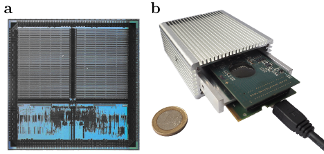
Figure 1: The neuromorphic hardware system Spikey. (a) Photograph of the Spikey chip (size $$5\text{\,}$\times$5\text{\,}{\mathrm{mm}}^{2}$$). It comprises analog circuits of $384$ neurons and $98304$ synapses, is highly configurable and emulates neural-network dynamics with a speed-up of $10^{4}$ with respect to biological real-time. (b) Photograph of the partly cased Spikey system, carrying the Spikey chip (covered by a black round seal) and conventional memory. The system is connected to the host computer via USB 2.0, consumes $6\text{\,}\mathrm{W}$ of power in total and less than $1\text{\,}\mathrm{nJ}$ per synaptic transmission (see Supplements 1).

In this study, we investigate the impact of heterogeneity on input and output correlations in the asynchronous regime of sparse networks of leaky integrate-and-fire (LIF) neurons with conductance-based synapses. Emulation of the networks on the analog neuromorphic hardware system Spikey (Figure 1) (Schemmel et al., 2006; Pfeil et al., 2013) enable us to investigate the impact of substrate specific properties on the network dynamics. Insights about the interplay between features of the computing substrate and network dynamics are a necessary prerequisite for the development of algorithms that exploit the benefits of analog neuromorphic systems at best. The configurability of this system (Pfeil et al., 2013) enables us to systematically vary the level of heterogeneity, and to disentangle the effects of heterogeneity on feedforward and feedback decorrelation (see above). For simplicity, we focus on purely inhibitory networks, thereby emphasizing that active decorrelation by inhibitory feedback does not rely on a dynamical balance between excitation and inhibition (Tetzlaff et al., 2012; Helias et al., 2014). We show that decorrelation by inhibitory feedback is effective even in highly heterogeneous networks with broad distributions of firing rates (Section III.1). Increasing the level of heterogeneity has two effects: Feedforward decorrelation is enhanced, feedback decorrelation is impaired. Due to the latter, the overall input and output correlations do not necessarily become smaller with increasing heterogeneity. They can even increase (Section III.2).

Note that results from specific network emulations on hardware do not directly translate to those obtained by simulations on conventional computers, because the dynamics, parametrization and interplay of analog circuits is very complex and difficult to reproduce with classical simulations. If simplified models for spatial and temporal variability are considered in software simulations, however, emulation results can be reproduced qualitatively, thereby verifying the design of the hardware system. While our hardware system is designed to physically implement biologically realistic neural algorithms in a fast and energy-efficient way, software simulations are used as a complementary tool to isolate, verify and investigate different hardware features, such as spatial and temporal parameter variations. Due to the limited access and configurability of network parameters, this would be difficult to achieve with hardware studies alone. In analogy to the necessity of performing experiments on biological neural systems to verify assumptions made in Computational Neuroscience, actual emulations on neuromorphic hardware are essential to understand its properties and develop efficient neural algorithms for these devices. The fact that our main findings hold true for both emulations on hardware and simulations with software, and that they can be distilled to simple linear models, support their broad relevance and robustness.

II Methods

II.1 Network model

Details on the network, neuron and synapse model are provided in Table 1. Parameter values are given in Table 2. Briefly: We consider a purely inhibitory, sparse network of $N$ ($N=192$, unless stated otherwise) LIF neurons with conductance-based synapses. Each neuron receives input from a fixed number $K=15$ of randomly chosen presynaptic sources, independently of the network size $N$. Self-connections and multiple connections between neurons are excluded. Resting potentials $E_{\text{l}}$ are set above the firing thresholds $\Theta$ (equivalent to applying a constant supra-threshold input current). We thereby ensure autonomous firing in the absence of any further external input. Due to temporal noise, the initial conditions are essentially random.

II.2 Network emulations on the neuromorphic-hardware system Spikey

The Spikey chip (Figure 1) consists of physical models of LIF neurons and conductance-based synapses with exponentially decaying dynamics (for details, see Table 1). The emergent dynamics of these physical models represents a solution for the model equations of neurons and synapses in continuous time, in parallel for all units. In contrast, in classical simulations on von-Neumann architectures, model equations are solved by step-wise numerical integration, where parallelization is limited by the available number of processor cores. To emphasize the difference between simulations using software and simulations using physical models, the term emulation is used for the latter (Pfeil et al., 2013).

The response properties of physical neurons and synapses vary across the chip due to unavoidable variations in the production process that manifest in a spatially disordered pattern (fixed-pattern noise). In contrast to the approximately static fixed-pattern noise, temporal noise, including electronic noise and transient experiment conditions (e.g., chip temperature), impairs the reproducibility of emulations. In general, two network emulations with identical configuration and stimulation do not result in identical network activity. Both fixed-pattern and temporal noise need to be taken into account when developing models for analog neuromorphic hardware.

The key features of the Spikey chip are the high acceleration and configurability of the analog network implementation. Some network parameters, e.g., synaptic weights and leak conductances, are configurable for each unit, while other parameters are shared for several units (for details see (Pfeil et al., 2013)). The hardware system is optimized for spike in- and output and allows to record the membrane potential of one (arbitrarily chosen) neuron with a sampling frequency of $96\text{\,}\mathrm{MHz}$ in hardware time. On the Spikey chip, capacitances are smaller and conductances are much higher than in biological nervous systems. In consequence, networks on the Spikey chip are emulated with a speed-up of approximately $10^{4}$ with respect to biological real-time. Due to this high acceleration of the neuromorphic chip, the data bandwidth of the connection between the neuromorphic system and the host computer is not sufficient to communicate with the chip in real time. Consequently, input and output spikes (for stimulation and from recordings, respectively) are buffered in a local memory next to the chip. The high acceleration of the Spikey chip allows most of the transistors to operate outside of weak inversion, thereby reducing the effect of transistor variations and minimizing fixed-pattern noise.

In contrast to such accelerated systems, most other configurable, analog neuromorphic substrates are designed for real-time emulations at very low power consumption (Badoni et al., 2006; Hafliger, 2007; Vogelstein et al., 2007; Indiveri et al., 2009; Serrano-Gotarredona et al., 2009; Brink et al., 2013; Benjamin et al., 2014) and implement fewer, but more complex, neurons (Renaud et al., 2010; Yu & Cauwenberghs, 2010).

Access to the Spikey system is encapsulated by the simulator-independent language PyNN (Davison et al., 2009; Brüderle et al., 2009), providing a stable and user-friendly interface. PyNN integrates the hardware into the computational neuroscience tool chain and has facilitated the implementation of several network models on the Spikey chip (Kaplan et al., 2009; Bill et al., 2010; Brüderle et al., 2010; Pfeil et al., 2013; Schmuker et al., 2014).

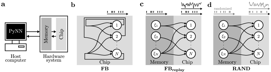
Figure 2: Experimental setup. (a) Data flow of the Spikey system. For details see Section II.2. (b) Network with on-chip feedback connections (FB). Spikes from all neurons are recorded to the local memory. (c) Spikes of the FB network in (b) replayed from memory via off-chip spike sources $\xi_{i}$ to neurons $i$ ($\text{FB}_{\text{replay}}$). Spike times of $\xi_{i}$ correspond to those recorded from neuron $i$ in (b). Spikes from all neurons or the free membrane potential of one selected neuron are recorded. (d) Like (c), but spike times from (b) are randomized for each source (RAND).

On the Spikey system, a spiking neural network is emulated as follows (Figure 2a): First, the network described in PyNN is mapped to the Spikey chip, i.e., neurons and synapses are allocated and parametrized. Second, input spikes, if available, are prepared on the host computer and transferred to the local memory on the hardware system. Third, the emulation is triggered and available input spikes are generated. Output spikes and membrane data are recorded to local memory. Last, spike and membrane data are transferred to the host computer and scaled back into the biological domain of the PyNN model description.

For consistency with the model description and simplified comparison to the existing literature, all hardware times and all hardware voltages are expressed in terms of the quantities they represent in the neurobiological model, throughout this study.

II.3 Experimental setup

To differentiate and compare the effects of shared inputs and feedback connections on correlations, we investigate two different emulation scenarios: First, we emulate networks with intact feedback (FB, Figure 2b), and second, the contribution of shared input is isolated by randomizing the temporal order of this feedback (RAND, Figure 2d).

In the RAND scenario, the inputs of neurons are decoupled from their outputs. Spatio-temporal correlations in presynaptic spike trains are removed by randomizing the presynaptic spike times.

Input correlations between neurons are measured via their free membrane potential, i.e., the membrane potential with disabled spiking mechanism (technically, the threshold is set very high). Because membrane potential traces can be recorded in the hardware only one at a time, traces are obtained consecutively, while repeatedly replaying the previously recorded activity of the FB network to a population of unconnected neurons of equal size. We keep the connectivity the same, and hence each neuron receives the same number of spikes as in the recurrent network during the whole emulation, either without ($\text{FB}_{\text{replay}}$, Figure 2c) or with randomization of presynaptic spike times (RAND, Figure 2d), respectively. To preserve the fixed pattern of variability of synaptic weights in hardware, the same hardware synapses are used for each connection in both scenarios. If network dynamics were reproduced perfectly, membrane potential traces and spike times would be identical in the FB and $\text{FB}_{\text{replay}}$ cases (see also Section II.4).

Drawing two different network realizations (i.e., the connectivity matrix) results in the allocation of different hardware synapses, and, due to fixed-pattern noise, in different values of synaptic weights. To average over this variability, throughout this study, emulation results are averaged over $M=100$ network realizations, if not stated otherwise.

II.4 Reproducibility of hardware emulations

Since the initial conditions of the recurrent network on hardware are undefined, consecutive emulations of the FB network result in different network activities. In the RAND and $\text{FB}_{\text{replay}}$ case, however, the input of neurons is decoupled from their output. Although unavoidable temporal noise is present, the system’s state-space trajectory returns to the trajectory of the previously recorded FB case. A certain degree of reproducibility is required for two reasons: First, the investigated effect of decorrelation by inhibitory feedback requires a precise relation between spike input and output. Thus our method of replacing the feedback loop by replay is only valid if temporal noise does not substantially corrupt this relationship. Second, to record the membrane potentials of all neurons, as if recorded at once, neuron dynamics have to be reasonably similar in consecutive emulations.

We measure the reproducibility of neuron dynamics by comparing consecutive emulations with identical configuration, i.e., connectivity and stimulation. For this purpose the spiking activity of a FB network is first recorded (Figure 2b) and then repeatedly replayed (Figure 2c). Reproducibility is quantified by the correlations ($\kappa_{X}$ in Table 3) of free membrane potential traces and output spike trains obtained for individual neurons in $L=25$ different trials.

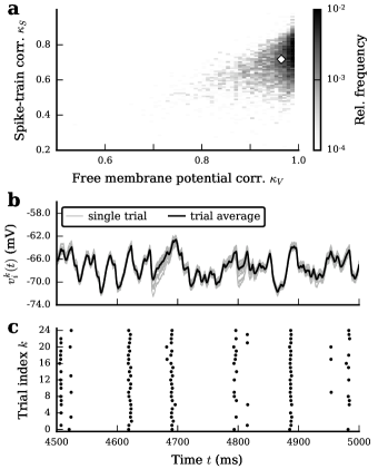
Figure 3: Reproducibility of free membrane potentials and spiking activity in the $\text{FB}_{\text{replay}}$ case. (a) Low-frequency coherence $\kappa_{{V}}$ and $\kappa_{{S}}$ of free membrane potentials $v_{i}^{k}(t)$ and $v_{i}^{l}(t)$ and binned spike trains $s_{i}^{k}(t)$ and $s_{i}^{l}(t)$, respectively, for each neuron $i$ averaged over $L=25$ trials $k,l$ with $k\neq l$, for $M=50$ different network realizations. The diamond marks the average across all neurons $i$ and $M$ network realizations ($\kappa_{{V}}=0.96$, $\kappa_{{S}}=0.72$). (b) Free single-trial membrane potentials $v_{i}^{k}(t)$ (gray) and average over trials $\frac{1}{L}\sum_{k=1}^{L}v_{i}^{k}(t)$ (black), and (c) spike density $\xi_{i}(t)$ of a single neuron $i$ for $L=25$ identical trials. The selected neuron $i$ has membrane potential coherence and spike train coherence closest to the diamond in (a).

Free membrane potentials are reproduced quite well, while spike trains show larger deviations across trials (Figure 3). Small deviations in the membrane potential (Figure 3b) are amplified by the thresholding procedure (Mainen & Sejnowski, 1995; De la Rocha et al., 2007; Wiechert et al., 2010) and can lead to large differences between spike trains (Figure 3c). Consequently, measures based on data of several consecutive replays are more precise for membrane potentials than for spike trains. Nevertheless, results have to be interpreted with care in both cases.

II.5 Calibration

The heterogeneity of the Spikey hardware is adjusted by calibrating the leak conductance for each individual neuron, compensating for fixed-pattern noise of neuron parameters. To this end, a population of unconnected neurons is driven by a constant supra-threshold current and the time-averaged population activity $\bar{r}$ is measured. Then, we applied the bisection method (Press et al., 2007) to adjust the leak conductance $g_{\text{l}}$ of each neuron, such that the neuron’s firing rate matches the target rate $\bar{r}$. This results in calibration values $b$ for the leak conductance $g_{\text{l}}=g_{\text{l,0}}(1+b)$, where $g_{\text{l,0}}$ is the leak conductance before calibration. Because emulations on hardware are not perfectly reproducible, more precise calibration was achieved by evaluating the median over $25$ identically configured trials instead of single trials. Furthermore, the bisection method was modified for noisy systems (for details, see Supplements 2).

Intermediate calibration states are obtained by linearly scaling the full calibration:

$$g_{\text{l}}=g_{\text{l,0}}(1+(1-a)b)\quad.$$ (1)

The heterogeneity $a$ is chosen in $[0,1]$ for calibrations between the uncalibrated ($a=1$) and calibrated state ($a=0$). In the following, the fully calibrated chip ($a=0$) is used, if not stated otherwise.

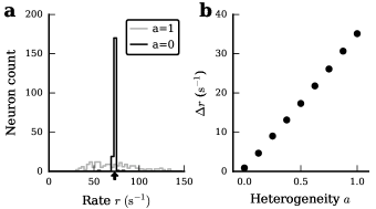
Figure 4: Calibration of the Spikey chip. (a) Histogram of firing rates $r$ for a population of unconnected neurons with supra-threshold input currents, before (gray) and after (black) calibration, each neuron averaged over $L=100$ trials. The arrow denotes the target rate $\bar{r}$. (b) Difference $\Delta r=r_{P75}-r_{P25}$ of 75th and 25th percentile of the histograms in (a), as a function of network heterogeneity $a$ (Equation 1). The mean firing rate over all values of $a$ is $73.4\pm 0.3\text{\,}{\mathrm{s}}^{-1}$.

This calibration substantially narrows the distribution of firing rates compared to the uncalibrated state (Figure 4). With respect to the stationary firing rate, variability on the neuron level is reduced from 35.1 to $$0.9\text{\,}\mathrm{s}$^{-1}$.

Even in the fully calibrated state, leak conductances can still be widely distributed. Due to the chosen calibration procedure, they are likely to be correlated to other parameters that influence the neurons’ response to a constant supra-threshold current after calibration. This mutual compensation can lead to similar phenomenology (here: firing rates) despite disparate parameter values, similar to what is observed in biology (Prinz et al., 2004). In addition to remaining variations in neuron parameters, synaptic parameters are significantly distributed (Pfeil et al., 2013; Schmuker et al., 2014).

II.6 Correlation measures

In the following, we introduce definitions used to analyze the recorded data. For clarity, all relevant equations and their parametrization are listed in Table 3 and 4, respectively.

We quantify correlations of membrane potentials $v_{i}(t)$ and spike trains $s_{i}(t)$ by the population-averaged low-frequency coherence $\kappa_{{V}}$ and $\kappa_{{S}}$, respectively. At frequency zero, the coherence corresponds to the normalized integral of the cross-covariance function, i.e., it measures correlations on all time scales. We define the low-frequency coherence $\kappa_{X}$, with $X\in\{S,V\}$, to be the average coherence over a frequency interval from $0.1\text{\,}$ to $20\text{\,}\mathrm{Hz}$. In this interval, the suppression of population-rate fluctuations in recurrent networks due to inhibitory feedback is most pronounced, and the coherence is approximately constant. Before calculating the coherence, we convolve the power- and cross-spectra with a rectangular window to average out random fluctuations. This measure, or a variant of it, is commonly used in the neuroscientific literature Bair et al. (2001); Kohn & Smith (2005); Moreno-Bote & Parga (2006); De la Rocha et al. (2007); Renart et al. (2010); Tetzlaff et al. (2012); Yim et al. (2013). We use the terms low-frequency coherence and correlation interchangeably.

Throughout this study, the term input correlations is used for correlations between free membrane potentials, and output correlations for correlations between spike trains. Shared-input correlations are membrane-potential correlations that are exclusively caused by overlapping presynaptic sources, ignoring possible correlations in the presynaptic activity. In homogeneous networks, the average pairwise shared-input correlation

$$\kappa_{{V}}=\frac{K}{N}$$ (2)

is given by the connectivity $K/N$ (Tetzlaff et al., 2012). In heterogeneous networks, shared-input correlations can be reduced. In the presence of heterogeneous synaptic weights, for example, the shared-input correlation

$$\kappa_{{V}}=\frac{1}{1+CV_{J}^{2}}\frac{K}{N}$$ (3)

is decreased by a factor $1/(1+CV_{J}^{2})$, where $CV_{J}$ denotes the coefficient of variation of the (non-zero) synaptic weights. Note, however, that heterogeneities which affect only the spike generation but not the integration of synaptic inputs, e.g. distributions of firing thresholds, have no effect on the shared-input correlation.

We assess the significance of correlations by comparing the results from emulations to correlations in surrogate data, in which we removed spatial correlations. For every neuron, we randomly shuffled bins of the membrane potential trace, and assigned a new timestamp uniformly drawn from the emulation interval to every spike, respectively. We thereby remove all spatio-temporal correlations between neurons recorded in parallel. By this procedure we create $100$ surrogate trials, across which we calculate the average correlations and the standard error.

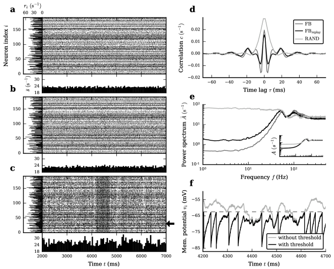
Figure 5: Typical spiking and membrane-potential activity of a random inhibitory network of LIF neurons with intact and cut feedback loop emulated on the fully calibrated system. (a–c) Spiking activity (raster plots), population activity $\bar{s}(t)$ (horizontal histograms; bin size $50\text{\,}\mathrm{ms}$) and time-averaged single-neuron firing rates $r_{i}$ (vertical histograms) in the network with intact feedback (a) and for cases where the feedback loop is cut (b and c). (a) Intact recurrent network (FB scenario). (b) Population of mutually unconnected neurons receiving input spike trains identical to those in (a) ($\text{FB}_{\text{replay}}$ scenario). (c) As in (b), but after randomization of presynaptic spike times (RAND scenario). (d,e) Population-averaged cross-correlation functions ${c}(\tau)$ (after offset subtraction) of pairs of spike trains (d) and power spectra $\bar{A}(f)$ (e; log-log representation) of the population activity $\bar{s}(t)$ (cf. horizontal histograms in (a–c)) for the FB (dark gray), $\text{FB}_{\text{replay}}$ (black) and RAND scenario (light gray). Inset in (e): Population-averaged power spectra $A(f)$ of individual single-cell spike trains (same scales as in main panel). Correlation functions and spectra are averaged across $M=100$ network realizations. (f) Membrane potential of a neuron in the RAND scenario (with firing rate of $23.20\text{\,}{\mathrm{s}}^{-1}$ close to population average of $23.24\text{\,}{\mathrm{s}}^{-1}$; see black arrow in (c)) with intact (black curve) and removed threshold (gray curve; free membrane potential). The threshold potential is marked by the horizontal dashed line. The time frame corresponds to the gray-shaded region in (c).

To quantify fluctuations in the population activity $\bar{s}$ (Figure 5a–c, horizontal histograms) we compute the power spectrum $\bar{A}(f)$ of the population activity (Figure 5e), which we scale with the duration $T$ of the emulation. Consequently, the population power spectrum $\bar{A}(f)$, scaled by the population size, coincides with the time-averaged population activity $\bar{r}$ for high frequencies: $\lim_{f\rightarrow\infty}\frac{1}{N}\bar{A}(f)=\bar{r}$ (Tetzlaff et al., 2008).

As a measure of pairwise correlations in the time domain (Figure 5d), we compute the population-averaged cross-correlation function ${c}(\tau)$ by Fourier transforming the population-averaged cross-spectrum $C(f)$ to time domain.

III Results

In this study, we investigate the roles of shared input, feedback and heterogeneity on input and output correlations in random, sparse networks of inhibitory LIF neurons with conductance-based synapses (Table 1), implemented on the analog neuromorphic hardware chip Spikey (Figure 1). Similarly to Tetzlaff et al. (2012), we separate the contributions of shared input and feedback by studying different network scenarios (Figure 2): In the FB case, we emulate the recurrent network with intact feedback loop (Figure 2b) and record its spiking activity (Figure 5a). In the $\text{FB}_{\text{replay}}$ case (Figure 2c), the feedback loop is cut and replaced by the activity recorded in the FB network. Ideally, the input to each neuron in the $\text{FB}_{\text{replay}}$ case should be identical to the input of the corresponding neuron in the FB network. As the replay of spikes and the resulting postsynaptic currents and membrane potentials are not perfectly reproducible on the Spikey chip, the neural responses in the FB and in the $\text{FB}_{\text{replay}}$ scenario are slightly different (compare Figures 5a and 5b). In the RAND case (Figures 2d and 5c), we use the same setup as in the $\text{FB}_{\text{replay}}$ case. However, the spike times in each presynaptic spike train are randomized. While the average presynaptic firing rates and the shared-input structure are exactly preserved in this scenario, the spatio-temporal correlations in the presynaptic spiking activity are destroyed.

Using this setup, we first demonstrate in Section III.1 that active decorrelation by inhibitory feedback Renart et al. (2010); Tetzlaff et al. (2012) is effective in heterogeneous networks with conductance-base synapses over a range of different network sizes. In Section III.2, we show that decreasing the level of heterogeneity by calibration of hardware neurons leads to an enhancement of this active decorrelation.

III.1 Decorrelation by inhibitory feedback

The time-averaged population activities in the FB, $\text{FB}_{\text{replay}}$ and RAND scenarios are roughly identical (vertical histograms in Figures 5a–c; see also high-frequency power in Figure 5e). In the FB and $\text{FB}_{\text{replay}}$ scenario, fluctuations in the population-averaged activity are small (horizontal histograms in Figure 5a and b). The removal of spatial and temporal correlations in the presynaptic spike trains in the RAND case leads to a significant increase in the fluctuations of the population-averaged response activity (horizontal histogram in Figure 5c). At low frequencies ($\leq$20\text{\,}\mathrm{Hz}$$), the population-rate power in the FB and in the RAND case differs by about two orders of magnitudes (dark and light gray curves in Figure 5e). This increase in low-frequency fluctuations in the RAND case is mainly caused by an increase in pairwise correlations in the spiking activity (Figure 5d; the power spectra of individual spike trains [inset in Figure 5e] are only marginally affected by a randomization of presynaptic spike times) Tetzlaff et al. (2012). In other words, shared-input correlations, i.e., those leading to large spike-train correlations in the RAND scenario, are efficiently suppressed by the feedback loop in the FB case.

On the neuromorphic hardware, the replay of network activity is not perfectly reproducible (Section II.4). While the across-trial variability in membrane potentials is small, postsynaptic spikes are dithered by few milliseconds (Figure 3). In the $\text{FB}_{\text{replay}}$ case, the suppression of shared-input correlations by correlations in presynaptic spike trains is slightly less efficient as compared to the intact network (FB). The differences in the population-rate power spectra and in the spike-train correlations between the $\text{FB}_{\text{replay}}$ and RAND case, respectively, are nevertheless substantial (solid black and light gray curves in Figure 5d and e; note the logarithmic scale; for a detailed investigation of spike dither see Supplements 4 and Supplements Figure 7).

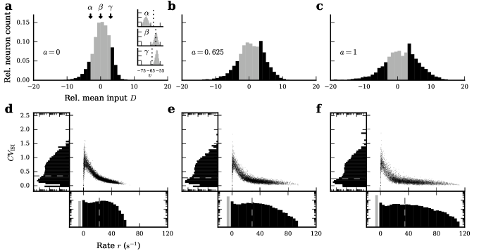
Figure 6: Modulation of network heterogeneity by leak-conductance calibration (see Section II.5). Input (top row) and firing statistics (bottom row) in the intact recurrent networks (FB scenarios) for fully calibrated (a and d; $a=0$), partially calibrated (b and e; $a=0.625$) and uncalibrated neurons (c and f; $a=1$). (a–c) Effect of calibration on input statistics. Distributions of relative mean input $D=(\bar{v}-\Theta)/\sigma(v)$ (distance of time averaged free membrane potential $\bar{v}$ from firing threshold $\Theta$ in units of the standard deviation $\sigma(v)$) across the population of neurons. Gray areas in (a), (b) and (c) highlight $[-3,3]$ intervals, containing $74\%$, $53\%$ and $42\%$ of the total mass of the distribution, respectively. Inset in (a): Distributions of free membrane potentials $v$ for three neurons $\alpha$, $\beta$ and $\gamma$ with $D=-3$, $D=0$ and $D=3$ (arrows in (a)), respectively. Dotted lines mark threshold potentials that may vary due to fixed-pattern noise. (d–f) Effect of calibration on spike-train statistics. Joint (scatter plots) and marginal distributions of single-neuron firing rates $r$ (horizontal histograms; log-linear scale) and coefficients of variation $CV_{\text{ISI}}$ of inter-spike intervals (vertical histograms; log-linear scale). Dashed lines mark mean of firing rate ($22.6\text{\,}{\mathrm{s}}^{-1}$, $28.7\text{\,}{\mathrm{s}}^{-1}$, $34.8\text{\,}{\mathrm{s}}^{-1}$) and $CV_{\text{ISI}}$ distributions ($0.35$, $0.28$, $0.25$), respectively. Gray bars (bottom panels) represent fractions of silent neurons. Data obtained from $M=50$ different network realizations. Percentage of dead neurons: $8\%,26\%,37\%$.

Note that the suppression of correlations and, hence, population-rate fluctuations by inhibitory feedback is restricted to low frequencies (here, to frequencies $<{}$50\text{\,}\mathrm{Hz}$$; see Figure 5e). In the remainder of this study, we will quantify pairwise correlations by the low-frequency coherence in the range $0.1\text{\,}$–$20\text{\,}\mathrm{Hz}$ (see Section II.6). At higher frequencies, the population-rate power spectra in the FB, $\text{FB}_{\text{replay}}$ and RAND case are similar. In Figure 5e, the peaks at $\sim{}$50\text{\,}\mathrm{Hz}$$ and higher harmonics result from the single-cell spike-train statistics (they are also visible in the single-cell spectra; see inset): A large fraction of cells, in particular those firing at higher rates, generate regular spike trains with low inter-spike-interval (ISI) variability (cf. Figure 6d–f). These (fast spiking) cells contribute maxima to the spike-train spectra at frequencies close to their firing rates (and higher harmonics). The structure of the population-rate spectra at higher frequencies ($\geq{}$50\text{\,}\mathrm{Hz}$$) is reproduced using surrogate data where the ISI distributions of the individual neurons (and, hence, their firing rates and ISI variability) are preserved, but serial ISI correlations and cross-correlations between spike trains are destroyed (data not shown).

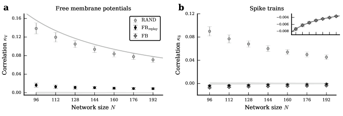
Figure 7: Dependence of population-averaged input correlations (a) and spike-train correlations (b) on the network size $N$, for the intact network (FB, dark gray diamonds), the $\text{FB}_{\text{replay}}$ (black circles) and the RAND (light gray circles) case (fixed in-degree $K=15$). Symbols and error bars denote mean and one standard deviation, respectively, across $M=100$ network realizations (error bars are partly covered by markers). The gray curve in (a) depicts shared-input correlations in a homogeneous network (Equation 2). The inset in (b) shows a magnified view of the spike-train correlations in the FB case (dark gray diamonds) with a power-law fit $\sim N^{-1}$ (dark gray curve). The light gray horizontal band represents mean $\pm$ three standard deviations of (spurious) correlations in surrogate data where correlations were removed. Note that free membrane potentials cannot be recorded in the FB case (see Section II). Hence, there are no gray diamonds in (a).

In the RAND case, presynaptic spike-train correlations were removed, and hence input (i.e., free-membrane-potential) correlations are exclusively determined by the number of shared presynaptic sources (Equation 2). If the in-degree $K$ is fixed, input correlations will decrease with network size $N$ (Equation 2, light gray curve and symbols in Figure 7a). In purely inhibitory networks with intact feedback loop (FB scenario), correlations in presynaptic spike trains are on average significantly smaller than zero (dark gray diamonds in Figure 7b, (Tetzlaff et al., 2012)), and largely cancel the positive contribution from shared-input correlations. Average input correlations are therefore significantly reduced (black symbols in Figure 7a). As both shared-input and spike-train correlations scale with the inverse of the network size ($N^{-1}$; light gray curve in Figure 7a and inset in Figure 7b, respectively) (De la Rocha et al., 2007), this suppression of correlations in the FB (and $\text{FB}_{\text{replay}}$) case is observed for all investigated network sizes $N$. Note that output correlations are negative even though input correlations are positive. This effect is predicted by theory and also observed in linear network models as well as LIF-network simulations on conventional computers (see Figure 9, Supplements 4, Supplements 5 and Section IV).

III.2 Effect of heterogeneity on decorrelation

In neural networks implemented in analog neuromorphic hardware, neuron and synapse parameters vary significantly across the population of cells (fixed-pattern noise; see Section II.2). For a population of mutually unconnected neurons with distributed parameters, injection of a constant (supra-threshold) input current leads to a distribution of response firing rates (Figure 4). In this study, we consider the width of this firing-rate distribution as a representation of neuron heterogeneity. It is systematically varied by calibration of leak conductances. The extent of heterogeneity is quantified by the calibration parameter $a$ ($a=1$ and $a=0$ correspond to the uncalibrated and the fully calibrated system, respectively; for details, see Section II.5). For an unconnected population of neurons subject to constant input, the width of the firing-rate distribution increases monotonically with $a$.

As shown in Figure 6, the level of heterogeneity (i.e., the calibration state $a$) is clearly reflected in the activity of the recurrent network (FB case). Both the width of the distribution of mean free membrane potentials (Figure 6a–c) as well as the width of the firing-rate distribution increases with $a$ (Figure 6d–f; horizontal histograms). In the uncalibrated system ($a=1$), a substantial fraction of neurons is predominantly driven by constant supra-threshold input currents and therefore generates highly regular spike trains ($CV_{\text{ISI}}\approx{}0$) with high firing rates ($r>$60\text{\,}\mathrm{s}$^{-1}$). Simultaneously, about $37\%$ of the neurons are silent ($r=$0\text{\,}\mathrm{s}$^{-1}$). Neurons with intermediate firing rates ($$0\text{\,}\mathrm{s}$^{-1}<r<$15\text{\,}\mathrm{s}$^{-1}$), however, show quite irregular activity ($CV_{\text{ISI}}>0.5$). After calibration, the firing-rate distribution is narrowed. For $a=0$, the fraction of silent neurons is reduced to about $8\%$. Maximum rates are limited to $<$66\text{\,}\mathrm{s}$^{-1}$. Note that our calibration routine compensates only for the distribution of neuron parameters, but not for the heterogeneity in synapse properties (synaptic weights, synaptic time constants; see Section IV). Even for the fully calibrated network ($a=0$), the firing-rate distribution is therefore still broad. In the RAND case, we obtain similar firing-rate and ISI statistics as in the FB case (Supplements 6).

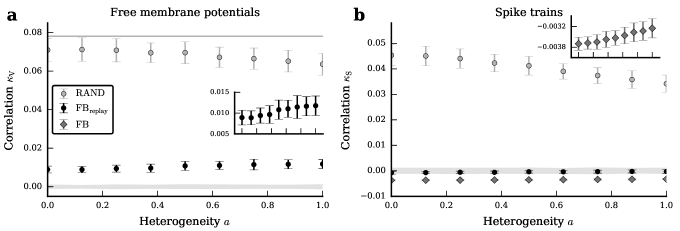
Figure 8: Dependence of population-averaged input correlations (a) and spike-train correlations (b) on the heterogeneity of the neuromorphic substrate for the intact network (FB, dark gray diamonds), the $\text{FB}_{\text{replay}}$ (black circles) and the RAND (light gray circles) case. Symbols and error bars denote mean and one standard deviation, respectively, across $M=100$ network realizations (error bars are partly covered by markers). The gray line in (a) depicts shared-input correlations in a homogeneous network (Equation 2). Insets in (a) and (b) depict magnified views of input correlations in the $\text{FB}_{\text{replay}}$ case and spike-train correlations in the FB case, respectively. The light gray horizontal band represents mean $\pm$ three standard deviations of (spurious) correlations in surrogate data where correlations were removed. Note that free membrane potentials cannot be recorded in the FB case (see Section II). Hence, there are no gray diamonds in (a).

For all levels of heterogeneity attainable by our calibration procedure ($a\in[0,1]$), input and output correlations are significantly suppressed by the recurrent-network dynamics (cf. black and dark gray vs. light gray symbols in Figure 8). In a homogeneous, random (Erdős-Rényi) network with fixed in-degree $K$ and linear sub-threshold dynamics, the contribution of shared input to the input (free-membrane-potential) correlation is given by the network connectivity $K/N$ (Equation 2; reference Tetzlaff et al., 2012) (thin light gray curves in Figure 7a and Figure 8a). Nonlinearities in synaptic and/or spike-generation dynamics (De la Rocha et al., 2007) as well as heterogeneity in neuron (and synapse) parameters lead to a suppression of this contribution (Equation 3, (Padmanabhan & Urban, 2010)). Here, we refer to this type of decorrelation as feedforward decorrelation. In fact, in our setup the input and spike-train correlations in the RAND case decrease with increasing heterogeneity (light gray symbols in Figure 8). Even in the fully calibrated case input correlations are slightly smaller than $K/N$ (gray symbols vs. thin gray curve in Figure 8a) due to remaining heterogeneities. Spike-train correlations decrease slightly faster with increasing heterogeneity than input correlations. These observations indicate that both the synaptic integration and spike generation are affected by heterogeneities on hardware. To illustrate the different effects of heterogeneity in synaptic integration and spike generation, we performed network simulations on conventional computers where we distributed either firing thresholds (Figure 9) or synaptic weights (Supplements Figure 4). In the RAND case, the decrease of input correlations on the hardware can be attributed to an increase in heterogeneity in parameters affecting synaptic integration (compare light gray symbols in Figure 8a and Supplements Figure 4a). Heterogeneity in spike thresholds, in contrast, does not affect input correlations in the RAND scenario, but strongly reduces spike-train correlations (light gray symbols in Figure 9). Overall, feedforward decorrelation, i.e. the suppression of correlations in the RAND case, becomes more effective in networks with heterogeneous cell parameters.

Despite this enhancement of feedforward decorrelation, input and output correlations increase with the level of heterogeneity in the presence of an intact feedback loop (FB and $\text{FB}_{\text{replay}}$ scenarios; black and dark gray symbols in Figure 8). We attribute this effect to a weakening of the effective feedback loop in the recurrent circuit: In heterogeneous networks with broad firing-rate distributions, neurons firing with low or high rates, corresponding to mean inputs far below or far above firing threshold (see Figure 6a–c), are less sensitive to input fluctuations than moderately active neurons (see Supplements Figure 2). Hence, they contribute less to the overall feedback. In consequence, feedback decorrelation is impaired by heterogeneity (see also Section IV).

IV Discussion

We have shown that inhibitory feedback effectively suppresses correlations in heterogeneous recurrent neural networks of leaky integrate-and-fire (LIF) neurons with nonlinear subthreshold dynamics, emulated on analog neuromorphic hardware (Spikey; (Schemmel et al., 2006; Pfeil et al., 2013)). Both input and output correlations are substantially smaller in networks with intact feedback loop (FB), as compared to the case where the feedback is replaced by randomized input while preserving the connectivity structure and presynaptic firing rates (RAND). Our results hence show that active decorrelation of network activity by inhibitory feedback (Renart et al., 2010; Tetzlaff et al., 2012) is a general phenomenon which can be observed in realistic, highly heterogeneous networks with nonlinear interaction and sufficiently strong negative feedback. Moreover, the study serves as a proof-of-principle that network activity can be efficiently decorrelated even on heterogeneous hardware, which can be exploited in functional applications, e.g., in the neuromorphic algorithms developed by Pfeil et al. (2013) and Schmuker et al. (2014).

Functional neural architectures often rely on stochastic dynamics of its constituents or on some form of background noise (see, e.g., Maass, 2014; Pfeil et al., 2013; Schmuker et al., 2014). Deterministic recurrent neural networks with inhibitory feedback could provide decorrelated noise to such functional networks, both in artificial as well as in biological substrates. In neuromorphic hardware applications, these “noise networks” could thereby replace conventional random-number generators and avoid a costly transmission of background noise from a host computer to the hardware substrate (which may be particularly relevant for mobile applications with low power consumption; see Supplements 1). It needs to be investigated, however, how well functional stochastic circuits perform in the presence of such network-generated noise.

Partial calibration of hardware neurons allowed us to modulate the level of network heterogeneity and, therefore, to systematically study its effect on correlations in the network activity. The analysis revealed two counteracting contributions: As shown in previous studies (e.g., Padmanabhan & Urban, 2010), neuron heterogeneity decorrelates (shared) feedforward input (feedforward decorrelation). On the other hand, however, heterogeneity impairs feedback decorrelation (see next paragraph). In our network model, this weakening of feedback decorrelation is the dominating factor. Overall, we observed a slight increase in correlations with increasing level of heterogeneity. We cannot exclude that feedforward decorrelation may play a more significant role for different network configurations (e.g., different connection strengths or network topologies, different structure of external inputs, different types of heterogeneity). Our study demonstrates, however, that heterogeneity is not necessarily suppressing correlations in recurrent systems. In this context, it would be interesting to investigate the interplay of signal and noise correlations in the presence of network heterogeneities in recurrent systems. We leave this intriguing topic to future studies.

As shown in (Tetzlaff et al., 2012), feedback decorrelation in recurrent networks becomes more (less) efficient with increasing (decreasing) strength of the effective negative feedback. For networks of spiking neurons, the effective connection strength $w_{ij}$ between two neurons $j$ and $i$ corresponds to the total number of extra spikes emitted by neuron $i$ in response to an additional input spike generated by neuron $j$ (see, e.g., (London et al., 2010)). Assuming that the effect of a single additional input spike is small, the effective connectivity can be obtained by linear-response theory (De la Rocha et al., 2007). Note that the effective weights $w_{ij}$ depend on the working point, i.e., the average firing rates of all pre- and postsynaptic neurons (mathematically, $w_{ij}$ is given by the derivative of the stationary response firing rate $r_{i}=\phi_{i}(r_{1},\ldots,r_{j},\ldots,r_{N})$ of neuron $i$ with respect to the input firing rate $r_{j}$, evaluated at the working point; for details, see (Tetzlaff et al., 2012)). Neurons firing at very low or very high rates are typically less sensitive to input fluctuations than neurons firing at intermediate rates (due to the shape of the response function $\phi_{i}(r_{1},\ldots,r_{N})$). Their dynamical range is reduced. In consequence, they hardly mediate feedback in a recurrent network. In heterogeneous networks with broad distributions of firing rates, the number of these insensitive neurons is increased. Hence, the effective feedback is weakened (see Supplements 3). We can qualitatively reproduce this effect of heterogeneity on correlations in recurrent networks (FB case) by means of a simplified linear rate model where increasing heterogeneity is described as a decrease in the effective-weight amplitudes (see Supplements 5). A more quantitative analysis requires an explicit mapping of the synaptic weights in the LIF-neuron network to the effective weights of the linear model (as in, e.g., (Grytskyy et al., 2013)) in the presence of distributed firing rates. We commit this task to future studies. Note that the rate dependence of the effective weights and the resulting effects on correlations are consistent with our observation that neuron pairs with very low firing rates exhibit spike-train correlations close to zero, whereas pairs with high firing rates are positively correlated (see Supplements 7). Pairs with one neuron firing at an intermediate rate often exhibit negative spike-train correlations. As shown in (Renart et al., 2010; Tetzlaff et al., 2012), these negative spike-train correlations are essential for compensating the positive contribution of shared inputs to the total input correlation (at least in purely inhibitory networks). Narrowing the firing rate distribution (e.g., by calibration of hardware neurons) increases the number of neurons contributing to the negative feedback, which, in turn, leads to more neuron pairs with negative spike-train correlations and, therefore, to smaller overall correlations.

Seemingly contrary to our findings, Bernacchia & Wang (2013) report a decrease in correlations with increasing level of heterogeneity. The results of their study are obtained for a linear network model, which can be considered the outcome of the linearization procedure described above. Hence, the connectivity of their model corresponds to an effective connectivity (see above). Their study neglects the rate (working-point) dependence of the effective weights and can therefore not account for the effect of firing-rate heterogeneity. In (Bernacchia & Wang, 2013), heterogeneity is quantified by the variance of the (effective) weight matrix (Equations 2.2 and 2.4 in (Bernacchia & Wang, 2013)). For sparse connectivity matrices (with a large number of zero elements), the variance of the weight matrix reflects not only the width of the non-zero-weight distribution, but also its mean (Equation 2.4 in (Bernacchia & Wang, 2013)). For networks of nonlinear spiking neurons, heterogeneities in neuron and/or synapse parameters broadens the distribution of non-zero effective weights, but may simultaneously reduce its mean (see above, Supplements 3, and (Roxin et al., 2011; Grytskyy et al., 2013)). Hence, the variance of the full weight matrix may decrease (for illustration, see Supplements Figure 9). In other words, increasing heterogeneity in the nonlinear system may correspond to decreasing heterogeneity in the linearized system. A direct test of this hypothesis requires an explicit linearization of the nonlinear heterogeneous system.

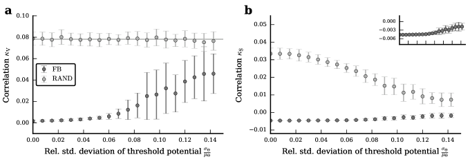
Figure 9: Dependence of population-averaged input correlations (a), and spike-train correlations (b) on the width of threshold distributions in networks simulated with NEST (Gewaltig & Diesmann, 2007) and PyNN (Davison et al., 2008), for the intact network (FB, dark gray circles) and the RAND (light gray circles) case. Symbols and error bars denote mean and standard deviation, respectively, across $M=30$ network realizations (error bars are partly covered by markers). The gray line in (a) depicts shared-input correlations in a homogeneous network (Equation 2). The inset in (b) shows a magnified view of the spike-train correlations in the FB case. Note that in simulations the $\text{FB}_{\text{replay}}$ is identical to the FB case, and is hence not shown. For details see Supplements 4.

The results of this study were obtained by network emulations on analog neuromorphic hardware. We reproduced the main findings by means of conventional computer simulations of LIF-neuron networks with distributed firing thresholds (see Figure 9). The focus on threshold heterogeneity allows us to isolate the effect of firing-rate distributions on correlations. It does not affect shared-input correlations (see Section II.6). Although networks simulated on conventional computers and those emulated on the neuromorphic hardware differ in several respects (e.g., in the exact implementation of heterogeneity or the synapse model; compare Supplements Table 1 and 2 to Table 1 and 2, respectively), the qualitative results are very similar: In networks with intact feedback loop, input and output correlations are substantially reduced (as compared to the case where the feedback is replaced by randomized input), but increase with the extent of heterogeneity. As predicted by the theory for homogeneous inhibitory networks, we observe positive input correlations and negative output correlations (see Equation $21$ in Tetzlaff et al. (2012) and in the paragraph which follows; see also Helias et al. (2013) and Supplements 5). Further, note that heterogeneity in neuron parameters does not “average out” in larger networks. Upscaling the network size by a factor of $25$ ($N=4800$, in-degree $K=375$) yields smaller spike-train correlations, but the qualitative results are similar to those obtained for the smaller network ($N=192$, $K=15$) emulated on the Spikey chip (compare Figure 8 to Supplements Figure 3).

In networks with intact feedback loop (FB and $\text{FB}_{\text{replay}}$ scenarios), the precise spatio-temporal structure of spike trains arranges such that the self-consistent input and output correlations are suppressed. Perturbations of this structure in the local input typically lead to an increase in correlations (Tetzlaff et al., 2012). In this study, we demonstrate this by replaying spiking activity after randomization of spike times, i.e., by replacing the time of each input spike by a random number uniformly drawn from the full emulation time interval $[0,T)$ (RAND case). However, even subtle modifications of input spike trains, such as random dither of spike times by few milliseconds, lead to an increase of correlations. On the neuromorphic hardware, replay of spike trains is not entirely reproducible (see Section II.4 and Supplements 9). Hence, spike-train correlations measured in the $\text{FB}_{\text{replay}}$ mode are slightly larger than in the FB case. We would expect the same effect on the input side (free membrane potentials). Due to hardware limitations, however, we can measure input correlations only in replay mode ($\text{FB}_{\text{replay}}$ or RAND), but not in the fully connected network (FB). Therefore, all reported input correlations are likely to be slightly overestimated. In conventional network simulations, we mimicked the effect of unreliable replay by input-spike dithering and, indeed, find a gradual increase in input and output correlations (see Supplements Figure 6). These results seem to be contrary to the study by Rosenbaum & Josic (2011), in which synaptic noise leads to a decrease of output correlations in a feedforward scenario. In our case, spike-train correlations, which suppress shared-input correlations, are removed by dithering spikes, thereby increasing correlations on the output side. In (Rosenbaum & Josic, 2011), in contrast, spike-train correlations are always zero, and shared-input correlations are decreased by synaptic failure, explaining the decreased output correlations. We attribute this contradiction to the missing feedback loop in their system, and expect correlations to increase in recurrent networks subject to similar perturbations.

Despite the imperfect replay of input spikes, the decorrelation effect is clearly visible in hardware emulations, both on the input and on the output side. The reproducibility of emulations on neuromorphic hardware could be improved by stabilizing the environment of the system, e.g., the chip temperature or the support electronics (under development). Analog hardware, however, will never reach the level of reproducibility of digital computers. But note that, similar to analog hardware, biological neurons exhibit a considerable amount of trial-to-trial variability, even under controlled in-vitro conditions (Mainen & Sejnowski, 1995). So far, the details of how neuronal noise, for example, stochastic synapses (spontaneous postsynaptic events, stochastic spike transmission, synaptic failure (Ribrault et al., 2011)), affects correlations in recurrent neural circuits remain unclear.

Although different Spikey chips exhibit different realizations of fixed-pattern noise, they show a comparable extent of heterogeneity and yield results which are qualitatively similar to those presented in this article (Supplements 8).

We have shown that negative feedback in recurrent circuits can efficiently suppress correlations, even in highly heterogeneous systems such as the analog neuromorphic architecture Spikey. Correlations can be further reduced by minimizing the level of network heterogeneity. In this study, we reduced the level of heterogeneity through calibration of neuron parameters in the unconnected case (see Section II.5). The calibration could, in principle, be improved by calibrating neuron (and possibly synapse) parameters in the full recurrent network. Such calibration procedures are however time consuming and cumbersome. In biological substrates, homeostasis mechanisms (Marder & Goaillard, 2006; O’Leary et al., 2014) keep neurons in a responsive regime and reduce the level of firing-rate heterogeneity in a self-regulating manner. Future neuromorphic devices could mimic this behavior, thereby reducing the necessity of time consuming calibration procedures. Alternatively, the analog circuits could be optimized to reduce fixed-pattern noise. This would likely require the allocation of more chip resources, hence reducing the network size per chip area.

For simplicity, this work focuses on purely inhibitory networks (as in (Mar et al., 1999)). This demonstrates that decorrelation by inhibitory feedback does not rely on a dynamical balance between excitation and inhibition (note that the external “excitatory” drive is constant in our model) (Tetzlaff et al., 2012; Helias et al., 2014). Previous studies have shown that, for the homogeneous case, decorrelation by inhibitory feedback is a general phenomenon, which also occurs in excitatory-inhibitory networks, provided the overall inhibition is sufficiently strong (which is typically the case to ensure stability) (Renart et al., 2010; Tetzlaff et al., 2012; Bernacchia & Wang, 2013; Helias et al., 2014). For the heterogeneous case, computer simulations of excitatory-inhibitory networks show qualitatively the same results as purely inhibitory networks (compare Figure 8 to Supplements Figure 5), confirming that our results generalize to the case of mixed excitatory-inhibitory coupling.

Similar to our study, Giulioni et al. (2012) use a theory-guided approach to implement, verify and investigate network dynamics on analog neuromorphic hardware. In their study, an attractor network is implemented that is inspired by a mean-field model. Due to heterogeneities in synaptic efficacies on the hardware, stability analysis of attractor states requires the authors to measure effective response functions of populations of hardware neurons. To this end, they replace recurrent connections in one population of neurons by external input. This allows them to measure the firing rate of the population as a function of the external input, while the activity of the population is in equilibrium with that of other recurrently connected populations. This study represents another example illustrating that investigations of actual hardware emulations are a prerequisite for successful application of analog neuromorphic hardware.

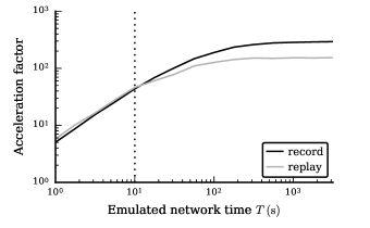
Figure 10: Acceleration factor as a function of emulated network time $T$ for the record (black) and the replay case (gray). The acceleration factor is defined as the ratio between the emulated network time $T$ (in biological time) and the execution time (wall clock time). In the record case, a network realization is generated on the host computer and uploaded to the chip. During the subsequent emulation, spike trains are recorded. In the replay case, spikes are replayed and the membrane potential of one neuron is recorded with full sampling frequency ($9.6\text{\,}\mathrm{kHz}$). The execution time covers the full data flow from a network description in PyNN to the emulation on the Spikey system and back to the network representation in PyNN. The time-averaged population firing rate is $\bar{r}=$23.7\pm 0.2\text{\,}{\mathrm{s}}^{-1}$$. The vertical dashed line depicts the runtime used in this study. The hardware system has to be initialized once before usage ($<$1\text{\,}\mathrm{s}$$), which is not considered here.

This study demonstrates that the Spikey system has matured to a level that permits its use as a tool for neuroscientific research. For the results presented in this study, we recorded in total $10^{11}$ membrane-potential and spike-train samples, representing more than $100$ days of biological time. Due to the $10^{4}$-fold acceleration of the Spikey chip, this corresponds to less than $15$ minutes in the hardware-time domain. Interfacing the hardware system, however, reduces the acceleration to an approximately $50$-fold speed-up (Figure 10). The translation between the network description and its hardware representation claims the majority of execution time, more than the network emulation and the transfer of data to and from the hardware system together. Encoding and decoding spike times on the host computer is particularly expensive. Obviously, the system could be optimized by processing the data directly on the hardware, or by choosing a data representation which is closer to the format used on the Spikey chip, but this would impair user-friendliness, and hence, the effectiveness of prototyping. While the Spikey system permits the monitoring of the spiking activity of all neurons simultaneously, access to the membrane potentials is limited to a single (albeit arbitrary) neuron in each emulation run. Monitoring of membrane potentials of a population of $n$ neurons therefore requires $n$ repetitions of the same emulation. Extending the hardware system to enable access to the membrane potentials of at least two neurons simultaneously would allow for a direct observation of input correlations in the intact network (and thereby avoid problems with replay reproducibility; see above) and reduce execution time (the Spikey chip itself permits recording of up to eight neurons in parallel, the support electronics, however, does not). While the Spikey system does not significantly outperform conventional computers in terms of computational power, emulations on this system are much more energy efficient (Supplements 1). A substantial increase of computational power is expected for large systems exploiting the scalability of this technology without slow-down (Schemmel et al., 2010).

Appendix A Network description

A                                                                          Model summary
Populations	One (inhibitory)
Topology	None
Connectivity	Random convergent connections (fixed in-degree)
Neuron model	Leaky integrate-and-fire (LIF), fixed firing threshold, fixed absolute refractory time
Channel models	None
Synapse model	Exponentially decaying conductances, fixed delays
Plasticity	None
External input	Resting potential higher than threshold (= constant current) ($E_{\text{l}}>\Theta$)
Measurements	Spikes and membrane potentials from all neurons
Other	No autapses, no multapses

B                                                                          Populations
Name	Elements	Size
I	LIF neuron	$N$

C                                                                          Connectivity
Source	Target	Pattern
I	I	Random convergent connections, in-degree $K$

D                                                                          Neuron and synapse model
Type	Leaky integrate-and-fire, exponentially decaying conductances
Subthreshold dynamics	Subthreshold dynamics ($t\not\in(t^{*},t^{*}+\tau_{\text{ref}})$):     $C_{\text{m}}\frac{\text{d}}{\text{d}t}v(t)=-g_{\text{l}}(v(t)-E_{\text{l}})-g_{\text{syn}}(t)(v(t)-E_{\text{inh}})$ Reset and refractoriness ($t\in(t^{*},t^{*}+\tau_{\text{ref}})$):     $v(t)=v_{\text{reset}}$ This model is emulated by analog circuitry on the Spikey chip (Indiveri et al., 2011).
Conductance dynamics	For each presynaptic spike at time $t^{*}$ ($t>t^{*}+d$):     $g_{\text{syn}}(t)\approx J\exp(-\frac{t-t^{*}-d}{\tau_{\text{syn}}})\Theta(t)$, with $J=w_{\text{hw}}g_{\text{max}}$ and Heaviside function $\Theta(t)$. This model is emulated by analog circuitry on the Spikey chip (Pfeil et al., 2013).
Spiking	If $v(t^{*}-)<\Theta\wedge v(t^{*}+)\geq\Theta$:     emit spike with time stamp $t^{*}$

Table 1: Description of the network model (according to (Nordlie et al., 2009)).

B                                                                          Populations
Name	Values	Description
$N$	$\{96,112,128,144,160,176,\textbf{192}\}$	network size
C                                                                          Connectivity
Name	Values	Description
$K$	$15$	number of presynaptic partners
D                                                                          Neuron
Name	Values	Description
$v_{\text{reset}}$	$-80\text{\,}\mathrm{mV}$	reset potential
$E_{\text{l}}$	$-52\text{\,}\mathrm{mV}$	resting potential
$\Theta$	$-62\text{\,}\mathrm{mV}$	firing threshold
$E_{\text{inh}}$	$-80\text{\,}\mathrm{mV}$	inhibitory reversal potential
$\tau_{\text{ref}}$	$1\text{\,}\mathrm{ms}$	refractory period
$C_{\text{m}}$	$0.2\text{\,}\mathrm{nF}$	membrane capacitance
$g_{\text{l}}$	tuned during calibration process	leak conductance
$\tau_{\text{m}}^{\text{\text{eff}}}$	uncalibrated: $10.50(5.94,17.90)$$\text{\,}\mathrm{ms}$	effective membrane time constant
	calibrated: $10.77(6.22,18.30)$$\text{\,}\mathrm{ms}$
D                                                                          Synapse
Name	Values	Description
$g_{\text{max}}$	in the order of $1\text{\,}\mathrm{nS}$	conductance amplitude
$w_{\text{hw}}$	$3$	synaptic weight (in hardware values $\in[0,15]$)
$V_{\text{max}}^{\text{\text{eff}}}$	uncalibrated: -$5.57(-12.50,-2.62)$$\text{\,}\mathrm{mV}$	effective post-synaptic potential prefactor
	calibrated: -$6.05(-14.37,-2.92)$$\text{\,}\mathrm{mV}$
$\tau_{\text{syn}}^{\text{\text{eff}}}$	uncalibrated: $3.78(2.52,5.58)$$\text{\,}\mathrm{ms}$	effective synaptic-current time constant
	calibrated: $4.17(2.76,6.18)$$\text{\,}\mathrm{ms}$
$d^{\text{\text{eff}}}$	uncalibrated: $2.16(1.91,2.48)$$\text{\,}\mathrm{ms}$	effective synaptic delay
	calibrated: $2.26(1.93,2.55)$
Other                                                                          Software
Name	Values	Description
SpikeyHAL	9e86d11c	git revision
PyNN	2fe40b43	git revision
vmodule	76ef3b44	git revision
logger	826c5ed6	git revision
Other                                                                          Hardware
Name	Values	Description
	chip 508 (version 5)	chip used for main manuscript
	chip 503, 504 (version 5) and 603, 605, 666 (version 4)	chips used for supplements

Table 2: Parameter values for the network model described in Table 1. Bold numbers indicate default values. Gray numbers indicate target values not considering fixed-pattern noise. Leak conductances $g_{\text{l}}$ are adjusted in the calibration process (see Section II.5). $\tau_{\text{m}}^{\text{\text{eff}}}$, $\tau_{\text{syn}}^{\text{\text{eff}}}$, $d^{\text{\text{eff}}}$ and $V_{\text{max}}^{\text{\text{eff}}}$ describe effective values measured from spike-triggered averages in RAND emulations as described in Supplements 10. Effective values denote the median across synapses and trials followed by the 25th and 75th percentiles in brackets.

Details on the network model as well as parameter values are provided in Table 1 and 2, respectively.

Appendix B Description of data analysis

A                                                                          Analysis measures
Measure	Details
spike density	$\xi_{i}(t)=\sum_{k}\delta(t-t_{i}^{k})$
spike train	$s_{i}(t_{k})=$ number of spikes of neuron $i$ per bin $[k\Delta t,(k+1)\Delta t)$
population activity	$\bar{s}(t)=\frac{1}{N}\sum_{i}s_{i}(t)$
time-averaged population activity	$\bar{r}=\left<\bar{s}(t)\right>_{t}$
membrane potential	$v_{i}(t_{k})=$ membrane potential of neuron $i$ in bin $[k\Delta t,(k+1)\Delta t)$
(finite time) Fourier transform	$X_{i}(f)=\mathfrak{F}[x_{i}(t)](f)=\int_{0}^{T}dt\,x_{i}(t)e^{-2\pi ift}$ (with inverse $\mathfrak{F}^{-1}$)
(single unit) power spectrum	$A_{i}(f)=\frac{1}{T}X_{i}^{*}(f)X_{i}(f)$
population-averaged power spectrum	$A(f)=\frac{1}{N}\sum_{i}A_{i}(f)$
population power spectrum	$\bar{A}(f)=\frac{1}{T}(\sum_{i}S_{i}^{*}(f))(\sum_{j}S_{j}(f))$
pairwise cross spectrum	$C_{ij}=\frac{1}{T}X_{i}^{*}(f)X_{j}(f),i\neq j$
population-averaged cross spectrum	$C(f)=\frac{1}{N(N-1)}\sum_{i\neq j}C_{ij}(f)\equiv\frac{1}{N(N-1)}(\bar{A}(f)-NA(f))$
	(note: $C(f)\in\mathbb{R}$)
sliding window filter	$X(f)\rightarrow X(f)\ast H(f)$
	with $H(f)=\frac{1}{f_{1}-f_{0}}\Theta(f-f_{0})\Theta(f_{1}-f)$
coherence	$\kappa(f)=\frac{C(f)}{A(f)}$
low-frequency coherence	$\kappa_{X}=\frac{1}{f_{\text{max}}-f_{\text{min}}}\int_{f_{\text{min}}}^{f_{\text{max}}}df\kappa(f)$
pop.-averaged cross-correlation function	${c}(\tau)=\frac{1}{N(N-1)}\sum_{i\neq j}\left<s_{i}(t)s_{j}(t+\tau)\right>_{t}\equiv\mathfrak{F}^{-1}[C(f)](\tau)$
time average	$\left<\dots\right>_{t}$

Table 3: Summary of the data analysis. Here $i\in[1,N]$, $X\in{S,V}$.

A                                                                          Analysis parameters
Parameter	Description	Values
$\Delta t$	bin size for spike trains	$1\text{\,}\mathrm{ms}$
$\Delta t_{\mathrm{m}}$	bin size for membrane potential traces	$0.52\text{\,}\mathrm{ms}$
$T_{\text{warmup}}$	initial warm-up time (not considered in analysis)	$1\text{\,}\mathrm{s}$
$T$	emulated network time (biol. time domain)	$10\text{\,}\mathrm{s}$
$M$	number of network realizations	$\{50,\textbf{100}\}$
$\Delta F$	width of sliding window	$1\text{\,}\mathrm{Hz}$
$f_{\text{min}},f_{\text{max}}$	interval boundaries for low-frequency coherence	$0.1\text{\,}\mathrm{Hz}$, $20\text{\,}\mathrm{Hz}$
$a$	calibration state	$\{0,\frac{1}{8},\frac{2}{8},\frac{3}{8},\frac{4}{8},\frac{5}{8},\frac{6}{8},\frac{7}{8},\textbf{1}\}$

Table 4: Summary of analysis parameters (default values in bold).

A summary of the quantities and the data analysis used in this study is provided in Table 3. Parameter values for the data analysis are given in Table 4.

Supplements

Supplements 1 Power consumption

The Spikey system consumes approximately $6\text{\,}\mathrm{W}$ of power, and the chip itself less than $0.6\text{\,}\mathrm{W}$. On the chip most power is consumed by digital communication infrastructure, which is not part of the neuromorphic network. In the following, we estimate the power consumption for a single synaptic event using the data set partly shown in Figure 5a. This emulation lasts $T=$10\text{\,}\mathrm{s}$$ in biological time and generates approximately $45\cdot 10^{3}$ spikes. Considering the acceleration of the hardware network ($10^{4}$) and the synapse count per neuron ($K=15$), the system generates $7\cdot 10^{8}$ synaptic events per second in hardware time. If we consider the total power consumption of the Spikey chip, the upper bound of energy consumed by each synaptic transmission will be approximately $1\text{\,}\mathrm{nJ}$. Because these measurements include the communication infrastructure and other support electronics to observe spike times and membrane traces, the real energy consumption for synaptic transmissions is estimated to be approximately ten times smaller. Network simulations on conventional supercomputers a far less energy efficient and consume tens of $\text{\,}\mathrm{\SIUnitSymbolMicro J}$ for each synaptic transmission (Sharp et al., 2012).

Supplements 2 Modification of the bisection method

In each iteration of the bisection method that is used to calibrate the leak conductances of hardware neurons (Section II.5), we evaluated the firing rate for each neuron by the median over $L=25$ identical trials. However, if this measure is compared between consecutive identical iterations, temporal noise on time scales longer than the duration of one iteration may still lead to variability. In the original bisection method, the interval of possible solutions is halved after each iteration step (Press et al., 2007). To improve the convergence of this method in the context of our calibration we expanded the halved interval by $20\%$ at both ends after each iteration. This prevents the algorithm to get stuck in an interval wrongly chosen by random fluctuations of the firing rates.

Supplements 3 Effective weights

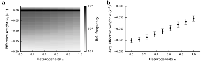
SUP. FIG. 1: Distribution of effective weights $w$ (a; log scale) and population-averaged effective weights $\bar{w}$ (b) for different levels of heterogeneity, averaged over $M=100$ network realizations. Symbols and error bars denote mean and one standard deviation, respectively.

We quantify the effect of a single spike of neuron $j$ on the firing rate of a postsynaptic neuron $i$ by the effective weight $w_{ij}$ of the connection $i\leftarrow j$. Assuming that the activity of neuron $i$ does not affect the activity of neuron $j$ (i.e., the RAND case), we define $w_{ij}$ as the cross-correlation between the spike trains $s_{j}(t)$ and $s_{i}(t+\tau)$, where, due to causality, $\tau$ is positive. Then, we average the effective weight over the emulated network time $T$, and subtract the baseline determined by the average correlation for negative $\tau$:

$$w_{ij}= \frac{1}{\tau_{\mathrm{max}}}\int_{0}^{\tau_{\mathrm{max}}}\langle s_{j}(t)s_{i}(t+\tau)\rangle_{t}d\tau-\frac{1}{\tau_{\mathrm{min}}}\int_{-\tau_{\mathrm{min}}}^{0}\langle s_{j}(t)s_{i}(t+\tau)\rangle_{t}d\tau\quad.$$ (S1)

Here, we chose $\tau_{\mathrm{max}}=$50\text{\,}\mathrm{ms}$$ and $\tau_{\mathrm{min}}=$50\text{\,}\mathrm{ms}$$. $\tau_{\mathrm{max}}$ was determined by measuring the average duration in which a spike from neuron $j$ has an influence on neuron $i$ (data not shown). $\tau_{\mathrm{min}}$ was then chosen symmetrically. The mass of the effective weights density shifts towards less negative effective weights for increasing heterogeneity (Supplements Figure 1a).

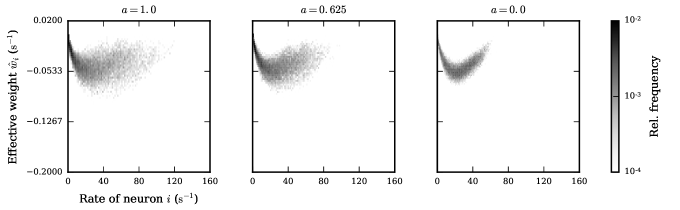
SUP. FIG. 2: Distribution of average incoming effective weights $\hat{w}_{i}$ over the rates of the postsynaptic neurons $i$, for three different levels of heterogeneity ($a=0$, $a=0.625$ and $a=1$), averaged over $M=100$ network realizations. The average incoming effective weights are obtained by summing over all presynaptic partners ($\hat{w}_{i}=\sum_{j}w_{ij}$).

We obtain $\bar{w}$ by averaging over all possible connections:

$$\bar{w}=\frac{1}{NK}\sum_{i,j}w_{ij}\quad.$$ (S2)

For increasing heterogeneity the absolute value of the average effective weight $\bar{w}$ decreases (Supplements Figure 1b). This can be explained by the dependence of the effective weight on the firing rate of the postsynaptic neuron (Supplements Figure 2). In the regime of small rates ($<$10\text{\,}\mathrm{s}$^{-1}$), incoming spikes hardly affect the neuron’s firing and the effective weight is small. Similarly, in the case for large rates ($>$40\text{\,}\mathrm{s}$^{-1}$). Neurons with intermediate firing rates are sensitive to input and hence have a more negative effective weight. Heterogeneity increases the number of neurons with small and large firing rates, and hence the absolute value of the average effective weight decreases, which in turn weakens the effective negative feedback of the network.

Supplements 4 Simulations with software

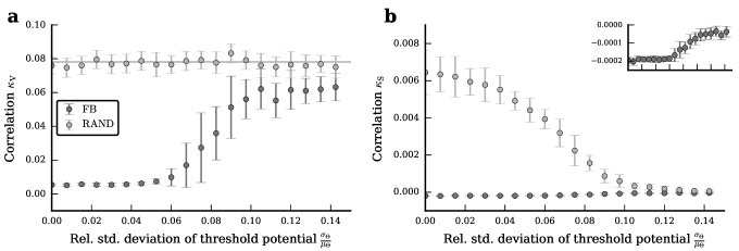
SUP. FIG. 3: Like Figure 9, but for $N=4800$ neurons and $K=375$ inputs for each neuron. Note the different scales of the ordinate in Figure 9 and (b). Symbols and error bars denote mean and standard deviation, respectively, across $M=20$ network realizations (error bars are partly covered by markers).

We validate our results by comparing them to simulations with software (NEST (Gewaltig & Diesmann, 2007), PyNN (Davison et al., 2008)). In these simulations we modulated the degree of heterogeneity by distributing the firing thresholds of all neurons according to a normal distribution with mean $\Theta$ and standard deviation $\sigma_{\Theta}$. Details about the network, neuron and synapse models and their parameters can be found in Supplements Table 1 and 2, respectively. The results are qualitatively similar to network emulations on the Spikey chip (compare Figure 8 to 9) and also hold for larger network sizes (Supplements Figure 3). In the FB case, input correlations and output correlations increase with network heterogeneity. In contrast to hardware emulations, input correlations stay approximately constant in the RAND case. Output correlations strongly decrease with the standard deviation $\sigma_{\Theta}$. Here, heterogeneity only affects the output spike times, and not the integrative properties of the neurons (see also Section III.2 and (Yim et al., 2013)).

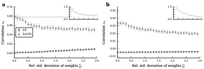
SUP. FIG. 4: Dependence of population-averaged input correlations (a), and spike-train correlations (b) on the width of the weight distribution, for the intact network (FB, dark gray circles) and the RAND (light gray circles) case. Symbols and error bars denote mean and standard deviation, respectively, across $M=30$ network realizations (error bars are partly covered by markers). The gray line in (a) depicts shared-input correlations in a homogeneous network (Equation 2). The insets show correlations normalized to unity at $\sigma_{J}=0$, with the same abscissa as in the main plot. Note that in simulations the $\text{FB}_{\text{replay}}$ is identical to the FB case, and is hence not shown. Networks simulated with NEST (Gewaltig & Diesmann, 2007) and PyNN (Davison et al., 2008).

In addition, we compare the effect of heterogeneity in firing thresholds on correlations to that of heterogeneity in synaptic weights. Details about the network, neuron and synapse models and their parameters can be found in Supplements Table 1 and 3, respectively. If we distribute synaptic weights, shared-input correlations decrease with the width of the weight distribution (Supplements Figure 4). Output correlations are also reduced, however, only proportionally to the reduction of input correlations (compare insets in Supplements Figure 4). While output correlations are overall smaller than input correlations due to the non-linearity in spike generation, we do not observe a boost of this decrease for large heterogeneities. Overall, the dynamics of the recurrent system is more sensitive to heterogeneities in firing thresholds than in synaptic weights (compare scale of abscissas of Figure 9 to Supplements Figure 4).

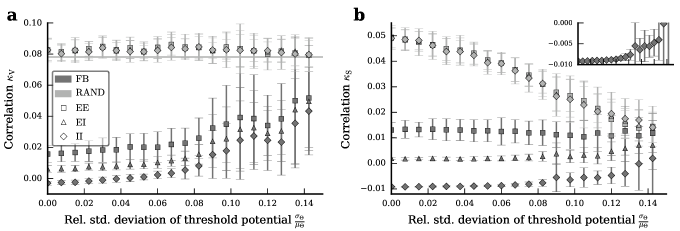
SUP. FIG. 5: Dependence of population-averaged input correlations (a), and spike-train correlations (b) on the width of the threshold distribution, for the intact network (FB, dark gray circles) and the RAND (light gray circles) case. The network consists of two populations, one excitatory and one inhibitory, of equal size. Symbols and error bars denote mean and standard deviation, respectively, across $M=30$ network realizations (error bars are partly covered by markers). The gray line in (a) depicts shared-input correlations in a homogeneous network (Equation 2). The inset in (b) shows a magnified view of the spike-train correlations in the FB case. Note that in simulations the $\text{FB}_{\text{replay}}$ is identical to the FB case, and is hence not shown. Networks are simulated with NEST (Gewaltig & Diesmann, 2007) and PyNN (Davison et al., 2008).

To investigate the generalization of our results to mixed excitatory-inhibitory networks, correlations were measured in a network of $N=192$ neurons consisting of half excitatory and half inhibitory neurons. Details about the network, neuron and synapse models and their parameters can be found in Supplements Table 4 and 5, respectively. As described above, we distribute the firing thresholds of all neurons according to a normal distribution. The results are consistent with those obtained from purely inhibitory networks on hardware demonstrating the generality of our findings (compare Figure 8 to Supplements Figure 5). By modulating the level of heterogeneity separately for the excitatory or the inhibitory population, we observe that network dynamics are more sensitive to heterogeneities in the inhibitory than in the excitatory population (data not shown).

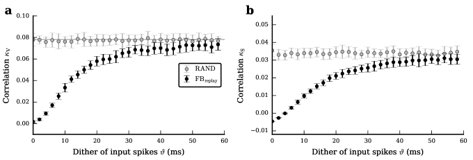
SUP. FIG. 6: Dependence of population-averaged input correlations (a), and spike-train correlations (b) on the strength of temporal noise, for the $\text{FB}_{\text{replay}}$ (black circles) and the RAND (light gray circles) case. Symbols and error bars denote mean and standard deviation, respectively, across $M=30$ network realizations (error bars are partly covered by markers). Gray curve in (a) depicts shared-input correlations in a homogeneous network (Equation 2). Correlations in the FB case correspond to correlations in the $\text{FB}_{\text{replay}}$ case for $\vartheta=$0\text{\,}\mathrm{ms}$$. Networks simulated with NEST (Gewaltig & Diesmann, 2007) and PyNN (Davison et al., 2008).

SUP. FIG. 7: Power spectrum of the population activity of the networks in Supplements Figure 6 for the intact network (solid dark gray), different degrees of dither on input spikes (dashed, dashed dotted and dotted black) and the RAND case (solid light gray), averaged across $M=30$ network realizations.

We investigate the effect of temporal noise on correlations by dithering spikes in the $\text{FB}_{\text{replay}}$ case before replaying them to the network (for network, neuron and synapse models see Supplements Table 1 and 2). Each spike time $t$ is replaced by a spike time $t^{\prime}$ randomly drawn from a normal distribution with width $\vartheta$: $t^{\prime}\sim\mathcal{N}(t,\vartheta)$. Even for small $\vartheta$, correlations increase on the input as well as on the output side, demonstrating the sensitivity of correlations to perturbations in the feedback loop (see Supplements Figure 6 and Tetzlaff et al. (2012)). This effect is also reflected in an increase of the power of the population activity at small frequencies (see Supplements Figure 7). These results suggest that on hardware temporal noise is responsible for the increase of correlations and population power in the $\text{FB}_{\text{replay}}$ case (compare $\text{FB}_{\text{replay}}$ to FB in Figure 5, 7 and 8).

Supplements 5 Linear model

We investigate the consistency of our results with a linear rate model that allows us to numerically calculate the average correlations from a given connectivity matrix ${\bf W}$. The model is defined as (according to, e.g., (Grytskyy et al., 2013))

$${\bf r}(t) =({\bf W}({\bf r}+{\bf x})\ast h)(t)\quad.$$ (S3)

Here, ${\bf r}(t)$ denotes the rate of the individual neurons and ${\bf x}(t)$ a Gaussian white noise input that is independent for each neuron. The linear filter kernel $h(t)$ depends on the details of the model, is not relevant in our calculation, and hence is not further specified here. Equation S3 can be transformed to Fourier domain, where the input and output spectral matrices can be expressed by

$${\bf C}_{\mathrm{RR}}(\omega) =T(\omega)T(\omega)^{\dagger}\quad,$$ (S4)

$${\bf C}_{\mathrm{RR}}^{\mathrm{in}}(\omega) ={\bf W}{\bf C}_{\mathrm{RR}}(\omega){\bf W}^{T}\quad,$$ (S5)

with $T(\omega)=(1-H(\omega){\bf W})^{-1}$ (Grytskyy et al., 2013). In the RAND case, the linear equation for the rate of the (unconnected) neurons reads

$${\bf q}(t)=({\bf W}(\tilde{{\bf r}}+{\bf x})\ast h)(t)\quad,$$ (S6)

where $\tilde{{\bf r}}(t)$ has the same auto-correlations as ${\bf r}(t)$ but zero cross correlations, i.e., ${\bf C}_{\mathrm{\tilde{R}\tilde{R}}}=\mathrm{diag}({\bf C}_{\mathrm{RR}})$, since the randomization of spike times removes all spatio-temporal correlations. According to Tetzlaff et al. (2012) spectral matrices in the RAND case are given by

$${\bf C}_{\mathrm{QQ}}^{\mathrm{in}}(\omega)= {\bf W}{\bf C}_{\mathrm{\tilde{R}\tilde{R}}}{\bf W}^{T}\quad,$$ (S7)

$${\bf C}_{\mathrm{QQ}}(\omega)= |H(\omega)|^{2}({\bf C}_{\mathrm{QQ}}^{\mathrm{in}}+\rho)\quad.$$ (S8)

We calculate the population-averaged power- and cross-spectra from the full matrices:

$$\bar{A}_{\mathrm{X}}(\omega) =\frac{1}{N}\sum_{i}C_{\mathrm{XX},ii}\quad,$$ (S9)

$$\bar{C}_{\mathrm{XX}}(\omega) =\frac{1}{N(N-1)}\sum_{i\neq j}C_{\mathrm{XX},ij}\quad.$$ (S10)

Here, $X\in\{R,Q\}$ denotes the FB and RAND case, respectively. The low frequency coherence is the cross-spectra normalized by the power spectra:

$$\kappa_{X}(0)=\frac{\bar{C}_{\mathrm{XX}}(0)}{\bar{A}_{\mathrm{X}}(0)}\quad.$$ (S11)

Note that in the linear model we are actually taking the zero frequency coherence.

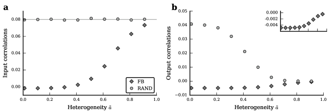
SUP. FIG. 8: Dependence of population-averaged input correlations (a), and output correlations (b) on the absolute magnitude of the effective weights (“heterogeneity” $\tilde{a}$, see text), for the intact network (FB, dark gray diamonds) and the RAND (light gray circles) case. Gray curve in (a) depicts shared-input correlations in a homogeneous network (Equation 2). The inset in (b) shows a magnified view of the spike-train correlations in the FB case (dark gray diamonds). Note that in the linear model the $\text{FB}_{\text{replay}}$ is identical to the FB case, and is hence not shown.

As in the spiking model, we consider a sparse network, i.e., we randomly choose for each neuron $i\in[1,N]$ an identical number of presynaptic partners ($K=15$). In the linear model we do not consider a distribution of non-zero effective weights. Instead, each realized connection is assigned the same weight value $-w$. To mimic the effect of calibration we vary the absolute value of the effective weight by scaling the weights of the non-zero connections with a sigmoidal function of $\tilde{a}\in[0,1]$:

$$\tilde{w}=\frac{1}{1+e^{10\times(\tilde{a}-0.5)}}w\quad.$$ (S12)

This procedure changes the variance of the weight matrix Bernacchia & Wang (2013) and hence $\tilde{a}$ is denoted the heterogeneity of the network. More homogeneous (heterogeneous) networks have larger (smaller) effective weights and hence stronger (weaker) feedback. We obtain qualitatively similar results as we observe on the Spikey chip (compare Supplements Figure 8 to Figure 8). Output correlations in the RAND case decrease, while both input and output correlations in the FB case increase with network heterogeneity, i.e., with the variance of the effective weight matrix. Note that, in this simplified model, input correlations in the RAND case are not affected by the level of "heterogeneity" because the non-zero weights are homogeneous, i.e. have zero variance, irrespectively of $\tilde{a}$ (cf. Equation 3).

SUP. FIG. 9: Distributions of effective weights in a sparse network. Different values for the mean $\mu_{\mathrm{w}}$ and standard deviation $\sigma_{\mathrm{w}}$ of the distribution of non-zero weights in (a) and (b), respectively, result in different values for the mean $\mu_{\mathrm{{W}}}$ and standard deviation $\sigma_{\mathrm{{W}}}$ of the effective weight matrix.

In Supplements Figure 9 we illustrate, how in a sparse network the variance of the weight matrix can increase, although the distribution of non-zero weights becomes narrower. The standard deviation $\sigma_{\mathrm{w}}$ of a distribution of non-zero weights with mean $\mu_{\mathrm{w}}$ is (in this example) smaller than the standard deviation $\sigma_{\mathrm{{W}}}$ of the full effective weight matrix, due to the sparseness of the matrix (Supplements Figure 9a; here, we chose $\epsilon=0.8$). If we, at the same time, increase the mean $\mu_{\mathrm{w}}$ and decrease the standard deviation $\sigma_{\mathrm{w}}$ of non-zero weights, the standard deviation of the weight matrix $\sigma_{\mathrm{{W}}}$ can increase significantly (Supplements Figure 9). While the distribution of effective weights is broadened, the mean is decreased, which has a greater impact on the size of correlations. This observation could explain the decrease of correlations with increased calibration of the neuromorphic chip.

Supplements 6 Firing statistics in the RAND case

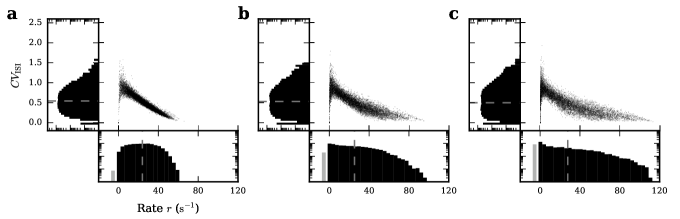
SUP. FIG. 10: (a–c) Like Figure 6d–f, but for the RAND case. The mean of firing rate ($24.0\text{\,}{\mathrm{s}}^{-1}$, $25.2\text{\,}{\mathrm{s}}^{-1}$, $27.8\text{\,}{\mathrm{s}}^{-1}$) and $CV_{\text{ISI}}$ distributions ($0.54$, $0.53$, $0.5$) are marked with dashed lines. Percentage of dead neurons: $0.00\%,0.02\%,0.08\%$.

The firing rate distributions in the RAND case are similar to those in the FB scenario (compare Supplements Figure 10 to Figure 6d–f). As in the FB case they become broader for increasing heterogeneity. Due to a larger variance of the membrane potentials, inactive neurons in the FB case have a higher probability to fire in the RAND case (compare gray bars in horizontal histograms of Supplements Figure 10a–c and Figure 6d–f). Neurons with firing rates larger than the average firing rate are strongly driven by constant current influx, and hence show similar firing rates than in the FB scenario. The irregularity of firing increases for the RAND compared to the FB case. This can also be traced back to an increased variance of the membrane potential for the RAND case (data not shown).

Supplements 7 Correlation matrices

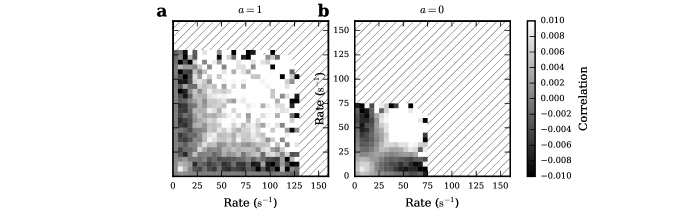
SUP. FIG. 11: Firing-rate dependence of pairwise low-frequency spike-train coherence in the uncalibrated (a) and fully calibrated system (b). Each bin represents the low-frequency spike-train coherence $\kappa_{ij}=\frac{1}{f_{\text{max}}-f_{\text{min}}}\int_{f_{\text{min}}}^{f_{\text{max}}}\frac{\mathfrak{Re}(C_{ij}(f))}{\sqrt{A_{i}(f)A_{j}(f)}}$, averaged across all neuron pairs $\{i,j\}$ with firing rates in the interval $[r_{i},r_{i}+\Delta{}r)$ and $[r_{j},r_{j}+\Delta{}r)$. Here, $\mathfrak{Re}(C_{ij}(f))$ denotes the real part of the complex cross-spectrum at frequency $f$. $f_{\text{min}}=$0.1\text{\,}\mathrm{Hz}$$, $f_{\text{max}}=$20\text{\,}\mathrm{Hz}$$, $\Delta{}r=$5\text{\,}\mathrm{s}$^{-1}$. Data averaged across $M=100$ network realizations.

In addition to the population-averaged measures from the main manuscript, we calculated the pairwise correlations for each pair $i,j$ of neurons with $i\neq j\in[1,N]$, and ordered these by the time-averaged rate of the corresponding neurons (Supplements Figure 11). This reveals a dependence of the pairwise correlation on the firing rate of the respective neurons. If both neurons fire at low rate (here $<$5\text{\,}{\mathrm{s}}^{-1}$$), correlations will be close to zero similar to the results in De la Rocha et al. (2007). For high rates (here $>$25\text{\,}{\mathrm{s}}^{-1}$$) we find mostly positive correlations. However, for neurons firing at intermediate rates, the activity of the pair is often anti-correlated, and can hence effectively suppress (positive) shared-input correlations. After calibration, the amount of neurons firing at intermediate rates and showing negative correlations increases (Supplements Figure 11b, Figure 6). Shared-input correlations are hence suppressed by more neurons leading to smaller input correlations than in the uncalibrated case (Figure 8).

Supplements 8 Results for different Spikey chips

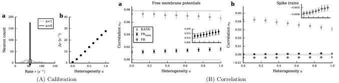
SUP. FIG. 12: Like Figure 4 and 8 in (A) and (B), respectively, but for two additional chips of version 5.

We have performed the same experiments as described in the main text using two additional Spikey chips of the current version (5). Different chips show different realizations of fixed-pattern noise, and hence calibration was repeated for each chip separately (Figure 4, Supplements Figure 12A). For all chips we find qualitatively the same results as described above: in the FB case, free membrane potentials (and spike trains) are decorrelated by inhibitory feedback and correlations increase with an increasing level of heterogeneity (Figure 8, Supplements Figure 12B).

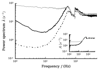
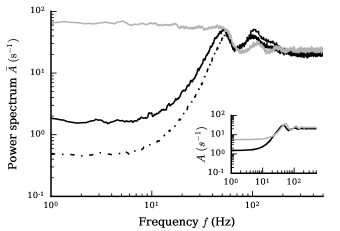
SUP. FIG. 13: Spectra of trial-averaged population power $\bar{A}(f)$ and trial-averaged single-cell power $A(f)$ for chip 666 (version 4, left) and chip 508 (version 5, right) illustrating the synchronization artifact in the $100\text{\,}\mathrm{Hz}$ range for the intact network (FB, dark gray), the $\text{FB}_{\text{replay}}$ (black) and the RAND (light gray) case.

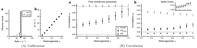
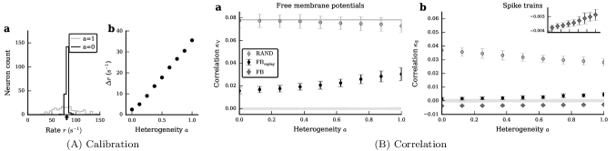
SUP. FIG. 14: Like Figure 4 and 8 in (A) and (B), respectively, but for three chips of version 4.

This also applies to the results of identical experiments on three previous-generation chips (version 4). These old chips show more pronounced heterogeneity in their parameters. In addition, we observe larger quantitative differences between old chips for the uncalibrated case, which is likely to be caused by different extents of intrinsic fixed-pattern noise. Unfortunately, the old systems show an artifact affecting the population power at around $100\text{\,}\mathrm{Hz}$ (Supplements Figure 13), consistently across all chips of identical revision. We can exclude that this effect can be traced back to network effects (it occurs across the FB, $\text{FB}_{\text{replay}}$ and RAND cases) or to single-cell power spectra (data not shown). We hence have to consider it an artificial spurious synchronization. As the artifact lies outside the range of frequencies that are relevant for our measures of correlation it does not affect the main results and experiments on the old chips qualitatively confirm our results in the main manuscript (compare Supplements Figure 14 to Figure 4, 8 and Supplements Figure 12).

Supplements 9 Reproducibility of networks with intact feedback

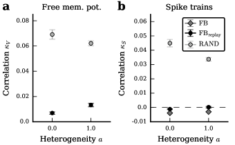
SUP. FIG. 15: Like Figure 8 and for the same chip, but for $L=20$ trials of one network realization.

We measured the standard deviation of free membrane potential and spike train correlations over several trials for a single network realization (Supplements Figure 15). This standard deviation is smaller than the standard deviation we observe over different network realizations (compare to Figure 8 and Supplements Figure 12), which indicates that the latter is mostly caused by the different realizations of the connectivity, not by trial-to-trial variability. Note that the variability between trials of networks with intact feedback is likely to be larger than between replays of network activity as shown in Figure 3, because network dynamics may be chaotic. The data shown in Supplements Figure 15 has to be interpreted with care, because the reproducibility of only a single network realization is considered. For different realizations, the mean and standard deviation will in general be different.

Supplements 10 Extraction of effective PSP amplitudes, time constants and delays

In order to provide an estimation for the order of magnitude of various neuron parameters, we fitted the postsynaptic potentials (PSPs) of current-based LIF neurons with exponential postsynaptic currents (PSCs) to the spike-triggered average (STA) of free membrane potentials obtained from hardware emulations. The differential equations describing the dynamics of membrane potentials $V_{j}(t)$ and synaptic currents $I_{j}(t)$ for this simplified model are given by

$$\tau_{\text{m}}^{\text{\text{eff}}}\dot{V}_{j}(t)= -V_{j}(t)+RI_{j}(t)$$ (S13)

$$\tau_{\text{syn}}^{\text{\text{eff}}}\dot{I}_{j}(t)= -I_{j}(t)+\tau_{\text{syn}}^{\text{\text{eff}}}\sum_{k}J_{jk}s_{k}(t-d^{\text{\text{eff}}})\,.$$ (S14)

where $R$ is the resistance of the membrane, $\tau_{\text{m}}^{\text{\text{eff}}}$ the membrane time constant, $\tau_{\text{syn}}^{\text{\text{eff}}}$ the synaptic time constant and $J_{jk}$ the synaptic weight of the connection from neuron $k$ to $j$. Here the superscript ${}^{\text{eff}}$ indicates that these are not the parameters realized on hardware, but of an abstract model that we fit to hardware measurements. Data were obtained from $100$ network realizations of the RAND case (same dataset as for Figure 8). For each neuron we computed the STA of its free membrane potential individually for each spike train of its presynaptic partners. The PSP for the current based model described above is given by

$$V(t)= V_{\text{max}}^{\text{\text{eff}}}\frac{\tau_{\text{syn}}^{\text{\text{eff}}}}{\tau_{\text{syn}}^{\text{\text{eff}}}-\tau_{\text{m}}^{\text{\text{eff}}}}\left(e^{-(t-d^{\text{\text{eff}}})/\tau_{\text{syn}}^{\text{\text{eff}}}}-e^{-(t-d^{\text{\text{eff}}})/\tau_{\text{m}}^{\text{\text{eff}}}}\right)\Theta(t-d^{\text{\text{eff}}})\,,$$ (S15)

where we introduced $V_{\text{max}}^{\text{\text{eff}}}=RJ$ to simplify the fitting procedure. For each pair of neurons $i$, $j$ we obtain a set of parameters: $V_{\text{max}}^{\text{\text{eff}}}$, $\tau_{\text{syn}}^{\text{\text{eff}}}$, $\tau_{\text{m}}^{\text{\text{eff}}}$ and $d^{\text{\text{eff}}}$.

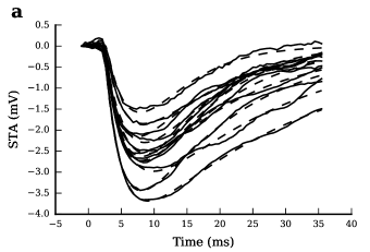
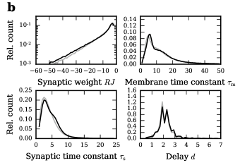
SUP. FIG. 16: (a) Fits of theoretical PSPs (dashed; for model, see Equation S15) to STAs of free membrane potentials in the FB case (solid). (b) Distributions of effective parameters obtained from fitting. Black and gray lines correspond to the fully calibrated ($a=0$) and uncalibrated ($a=1$) network, respectively. Median, 25th and 75th percentile of all fitted parameters are reported in Table 2.

The fitted curves (using the function scipy.optimize.curve_fit with default parameters from Python’s scipy module v0.17.0) match fairly well to the empirical data to allow an estimation of the effective values of the neuron parameters governing the shape of the postsynaptic potentials (Supplements Figure 16a). However, note that the resulting parameter distributions do not precisely reflect the actual parameter distributions on the chip.

The distributions of neuron and synapse parameters change slightly with calibration. For the calibrated network the absolute values of $V_{\text{max}}^{\text{\text{eff}}}$, $\tau_{\text{syn}}^{\text{\text{eff}}}$, $\tau_{\text{m}}^{\text{\text{eff}}}$ and $d^{\text{\text{eff}}}$ are larger than for the uncalibrated network (see Table 2 and Supplements Figure 16b).

A                                                                          Model summary
Populations	One (inhibitory)
Topology	-
Connectivity	Random convergent connections (fixed in-degree)
Neuron model	Leaky integrate-and-fire (LIF), fixed firing threshold, fixed absolute refractory time
Channel models	-
Synapse model	Exponentially decaying currents, fixed delays
Plasticity	-
External input	Resting potential higher than threshold (= constant current) ($E_{\text{l}}>\Theta$)
Measurements	Spikes and membrane potentials
Other	No autapses, no multapses

B                                                                          Populations
Name	Elements	Size
I	LIF neuron	$N$

C                                                                          Connectivity
Source	Target	Pattern
I	I	Random convergent connect, in-degree $K$

D                                                                          Neuron and synapse model
Type	Leaky integrate-and-fire, exponential currents
Subthreshold dynamics	Subthreshold dynamics ($t\not\in(t^{*},t^{*}+\tau_{\text{ref}})$):     $C_{\text{m}}\frac{\text{d}}{\text{d}t}v(t)=-g_{\text{l}}(v(t)-E_{\text{l}})+I_{\text{syn}}(t)$ Reset and refractoriness ($t\in(t^{*},t^{*}+\tau_{\text{ref}})$):     $v(t)=v_{\text{reset}}$
Current dynamics	$\tau_{\text{syn}}\frac{\text{d}}{\text{d}t}I_{\text{syn}}(t)=-I_{\text{syn}}(t)+\sum_{i,k}J\delta(t-t_{i}^{k})$ Here the sum over $i$ runs over all presynaptic neurons and the sum over $k$ over all spike times of the respective neuron $i$
Spiking	If $v(t^{*}-)<\Theta\wedge v(t^{*}+)\geq\Theta$:     emit spike with time stamp $t^{*}$

E                                                                          Measurements
Spike trains	recorded from $P_{\mathrm{s}}$ neurons
Membrane potentials	recorded from $P_{\mathrm{v}}$ neurons

SUP. TABLE 1: Description of the network model (according to (Nordlie et al., 2009)).

B                                                                          Populations
Name	Values	Description
$N$	$\{192,4800\}$	network size
C                                                                          Connectivity
Name	Values	Description
$K$	$\{15,375\}$	number of presynaptic partners
D                                                                          Neuron
Name	Values	Description
$C_{\text{m}}$	$0.2\text{\,}\mathrm{nF}$	membrane capacitance
$\tau_{\text{ref}}$	$0.1\text{\,}\mathrm{ms}$	refractory period
$v_{\text{reset}}$	$-80\text{\,}\mathrm{mV}$	reset potential
$E_{\text{l}}$	$-52\text{\,}\mathrm{mV}$	resting potential
$\Theta$	$\sim\mathcal{N}\left(-62,[0,8.8]\right)$ $\text{\,}\mathrm{mV}$	firing threshold
$g_{\text{l}}$	$10\text{\,}\mathrm{nS}$	leak conductance
D                                                                          Synapse
Name	Values	Description
$\tau_{\text{syn}}$	$5\text{\,}\mathrm{ms}$	synaptic time constant
$J$	$-0.254\text{\,}\mathrm{nA}$	synaptic weight
$d$	$1.0\text{\,}\mathrm{ms}$	synaptic delay
E                                                                          Measurements
Name	Values	Description
$P_{\mathrm{s}}$	$\{192,4800\}$	number of neurons spike trains are recorded from
$P_{\mathrm{v}}$	$\{150,150\}$	number of neurons membrane potentials are recorded from

SUP. TABLE 2: Parameter values for the network model described in Supplements Table 1 with distributed thresholds.

B                                                                          Populations
Name	Values	Description
$N$	$192$	network size
C                                                                          Connectivity
Name	Values	Description
$K$	$15$	number of presynaptic partners
D                                                                          Neuron
Name	Values	Description
$C_{\text{m}}$	$0.2\text{\,}\mathrm{nF}$	membrane capacitance
$\tau_{\text{ref}}$	$0.1\text{\,}\mathrm{ms}$	refractory period
$v_{\text{reset}}$	$-80\text{\,}\mathrm{mV}$	reset potential
$E_{\text{l}}$	$-52\text{\,}\mathrm{mV}$	resting potential
$\Theta$	$-62\text{\,}\mathrm{mV}$	firing threshold
$g_{\text{l}}$	$10\text{\,}\mathrm{nS}$	leak conductance
D                                                                          Synapse
Name	Values	Description
$\tau_{\text{syn}}$	$5\text{\,}\mathrm{ms}$	synaptic time constant
$J$	$\sim\left[\mathcal{N}\left(0.254,[0.00254,0.75]\right)\right]_{+}$	synaptic weight, clipped to positive values
$d$	$1.0\text{\,}\mathrm{ms}$	synaptic delay
E                                                                          Measurements
Name	Values	Description
$P_{\mathrm{s}}$	192	number of neurons spike trains are recorded from
$P_{\mathrm{v}}$	150	number of neurons membrane potentials are recorded from

SUP. TABLE 3: Parameter values for the network model described in Supplements Table 1 with distributed weights.

A                                                                          Model summary
Populations	Two (excitatory, inhibitory)
Topology	-
Connectivity	Random convergent connections (fixed in-degree)
Neuron model	Leaky integrate-and-fire (LIF), fixed firing threshold, fixed absolute refractory time
Channel models	-
Synapse model	Exponentially decaying currents, fixed delays
Plasticity	-
External input	Resting potential higher than threshold (= constant current) ($E_{\text{l}}>\Theta$)
Measurements	Spikes and membrane potentials
Other	No autapses, no multapses

B                                                                          Populations
Name	Elements	Size
E	LIF neuron	$N_{\text{E}}$
I	LIF neuron	$N_{\text{I}}$

C                                                                          Connectivity
Source	Target	Pattern
E	E	Random convergent connect, in-degree $K_{\text{E}}$, weight $J_{\text{E}}$
E	I	Random convergent connect, in-degree $K_{\text{E}}$, weight $J_{\text{E}}$
I	E	Random convergent connect, in-degree $K_{\text{I}}$, weight $J_{\text{I}}$
I	I	Random convergent connect, in-degree $K_{\text{I}}$, weight $J_{\text{I}}$

D                                                                          Neuron and synapse model
Type	Leaky integrate-and-fire, exponential currents
Subthreshold dynamics	Subthreshold dynamics ($t\not\in(t^{*},t^{*}+\tau_{\text{ref}})$):     $C_{\text{m}}\frac{\text{d}}{\text{d}t}v(t)=-g_{\text{l}}(v(t)-E_{\text{l}})+I_{\text{syn}}(t)$ Reset and refractoriness ($t\in(t^{*},t^{*}+\tau_{\text{ref}})$):     $v(t)=v_{\text{reset}}$
Current dynamics	$\tau_{\text{syn}}\frac{\text{d}}{\text{d}t}I_{\text{syn}}(t)=-I_{\text{syn}}(t)+\sum_{i,k}J\delta(t-t_{i}^{k})$ Here the sum over $i$ runs over all presynaptic neurons and the sum over $k$ over all spike times of the respective neuron $i$
Spiking	If $v(t^{*}-)<\Theta\wedge v(t^{*}+)\geq\Theta$:     emit spike with time stamp $t^{*}$

E                                                                          Measurements
Spike trains	recorded from $P_{\mathrm{s}}^{\text{E}}$ excitatory and $P_{\mathrm{s}}^{\text{I}}$ inhibitory neurons
Membrane potentials	recorded from $P_{\mathrm{v}}^{\text{E}}$ excitatory and $P_{\mathrm{v}}^{\text{I}}$ inhibitory neurons

SUP. TABLE 4: Description of the network model consisting of an excitatory and an inhibitory population (according to (Nordlie et al., 2009)).

B                                                                          Populations
Name	Values	Description
$N_{\text{E}}$	$96$	size of the excitatory population
$N_{\text{I}}$	$96$	size of the inhibitory population
C                                                                          Connectivity
Name	Values	Description
$K_{\text{E}}$	$7$	number of excitatory presynaptic partners
$K_{\text{I}}$	$8$	number of inhibitory presynaptic partners
D                                                                          Neuron
Name	Values	Description
$C_{\text{m}}$	$0.2\text{\,}\mathrm{nF}$	membrane capacitance
$\tau_{\text{ref}}$	$0.1\text{\,}\mathrm{ms}$	refractory period
$v_{\text{reset}}$	$-80\text{\,}\mathrm{mV}$	reset potential
$E_{\text{l}}$	$-52\text{\,}\mathrm{mV}$	resting potential
$\Theta$	$-62\text{\,}\mathrm{mV}$	firing threshold
$g_{\text{l}}$	$10\text{\,}\mathrm{nS}$	leak conductance
D                                                                          Synapse
Name	Values	Description
$\tau_{\text{syn}}$	$5\text{\,}\mathrm{ms}$	synaptic time constant
$J_{\text{E}}$	$0.0635\text{\,}\mathrm{nA}$	excitatory synaptic weight
$J_{\text{I}}$	$-0.254\text{\,}\mathrm{nA}$	inhibitory synaptic weight
$d$	$1.0\text{\,}\mathrm{ms}$	synaptic delay
E                                                                          Measurements
Name	Values	Description
$P_{\mathrm{s}}^{\text{E}}$	96	number of excitatory neurons spike trains are recorded from
$P_{\mathrm{s}}^{\text{I}}$	96	number of inhibitory neurons spike trains are recorded from
$P_{\mathrm{v}}^{\text{E}}$	150	number of excitatory neurons membrane potentials are recorded from
$P_{\mathrm{v}}^{\text{I}}$	150	number of inhibitory neurons membrane potentials are recorded from

SUP. TABLE 5: Parameter values for the network model described in Supplements Table 4.

References

- Gierer & Meinhardt (1974) Gierer, A., & Meinhardt, H. (1974). Biological pattern formation involving lateral inhibition. Lectures on mathematics in the life sciences 7, 163.
- Rosenzweig (1978) Rosenzweig, M. L. (1978). Competitive speciation. Biological Journal of the Linnean Society 10(3), 275–289.
- Neel (1952) Neel, L. (1952). Antiferromagnetism and ferrimagnetism. Proceedings of the Physical Society. Section A 65(11), 869.
- Renart et al. (2010) Renart, A., De La Rocha, J., Bartho, P., Hollender, L., Parga, N., Reyes, A., & Harris, K. D. (2010). The asynchronous state in cortical circuits. Science 327, 587–590.
- Tetzlaff et al. (2012) Tetzlaff, T., Helias, M., Einevoll, G., & Diesmann, M. (2012). Decorrelation of neural-network activity by inhibitory feedback. PLoS Comput. Biol. 8(8), e1002596.
- Helias et al. (2014) Helias, M., Tetzlaff, T., & Diesmann, M. (2014). The correlation structure of local cortical networks intrinsically results from recurrent dynamics. PLoS Comput. Biol. 10(1), e1003428.
- Pearson (1901) Pearson, K. (1901). Liii. on lines and planes of closest fit to systems of points in space. Philosophical Magazine Series 6 2(11), 559–572.
- Ginis & Peng (2006) Ginis, G., & Peng, C.-N. (2006). Alien crosstalk cancellation for multipair digital subscriber line systems. EURASIP Journal on Advances in Signal Processing 2006(1), 1–12.
- Benesty et al. (2001) Benesty, J., Gänsler, T., Morgan, D. R., Sondhi, M. M., & Gay, S. L. (2001). Advances in Network and Acoustic Echo Cancellation (1 ed.). Berlin, Germany: Springer.
- Trichina et al. (2001) Trichina, E., Bucci, M., De Seta, D., & Luzzi, R. (2001). Supplemental cryptographic hardware for smart cards. Micro, IEEE 21(6), 26–35.
- Mar et al. (1999) Mar, D., Chow, C., Gerstner, W., Adams, R., & Collins, J. (1999). Noise shaping in populations of coupled model neurons. Proc. Nat. Acad. Sci. USA 96(18), 10450–10455.
- Mead (1990) Mead, C. (1990). Neuromorphic electronic systems. Proc. IEEE 78(10), 1629–1636.
- Indiveri et al. (2011) Indiveri, G., Linares-Barranco, B., Hamilton, T. J., van Schaik, A., Etienne-Cummings, R., Delbruck, T., Liu, S.-C., Dudek, P., Häfliger, P., Renaud, S., Schemmel, J., Cauwenberghs, G., Arthur, J., Hynna, K., Folowosele, F., Saighi, S., Serrano-Gotarredona, T., Wijekoon, J., Wang, Y., & Boahen, K. (2011). Neuromorphic silicon neuron circuits. Front. Neurosci. 5(73).
- SenseMaker (2009) SenseMaker (2009). SenseMaker: A multi-sensory, task-specific, adaptable perception system; project website. Available at: http://cordis.europa.eu/project/rcn/62746_en.html.
- FACETS (2010) FACETS (2010). Fast Analog Computing with Emergent Transient States, project website. Available at: http://www.facets-project.org.
- BrainScaleS (2014) BrainScaleS (2014). Project website. Available at: http://www.brainscales.eu.
- Human Brain Project (2014) Human Brain Project (2014). Project website. Available at: http://www.humanbrainproject.eu.
- Pfeil et al. (2013) Pfeil, T., Grübl, A., Jeltsch, S., Müller, E., Müller, P., Petrovici, M. A., Schmuker, M., Brüderle, D., Schemmel, J., & Meier, K. (2013). Six networks on a universal neuromorphic computing substrate. Front. Neurosci. 7(11).
- Schmuker et al. (2014) Schmuker, M., Pfeil, T., & Nawrot, M. P. (2014). A neuromorphic network for generic multivariate data classification. Proc. Natl. Acad. Sci. USA 111(6), 2081–2086.
- Ecker et al. (2011) Ecker, A. S., Berens, P., Tolias, A. S., & Bethge, M. (2011). The effect of noise correlations in populations of diversely tuned neurons. J. Neurosci. 31(40), 14272–14283.
- Averbeck et al. (2006) Averbeck, B. B., Latham, P. E., & Pouget, A. (2006). Neural correlations, population coding and computation. Nat. Rev. Neurosci. 7, 358–366.
- Moreno-Bote et al. (2014) Moreno-Bote, R., Beck, J., Kanitscheider, I., Pitkow, X., Latham, P., & Pouget, A. (2014). Information-limiting correlations. Nat. Neurosci. 17, 1410–1417.
- Fries (2005) Fries, P. (2005). A mechanism for cognitive dynamics: neuronal communication through neuronal coherence. Theor. Comput. Sci. 9(10), 474–480.
- Abeles (1991) Abeles, M. (1991). Corticonics: Neural Circuits of the Cerebral Cortex (1st ed.). Cambridge: Cambridge University Press.
- Diesmann et al. (1999) Diesmann, M., Gewaltig, M.-O., & Aertsen, A. (1999). Stable propagation of synchronous spiking in cortical neural networks. Nature 402(6761), 529–533.
- Tabareau et al. (2010) Tabareau, N., Slotine, J.-J., & Pham, Q.-C. (2010). How synchronization protects from noise. PLoS Comput. Biol. 6(1). doi:10.1371/journal.pcbi.1000637.
- Salinas & Sejnowski (2001) Salinas, E., & Sejnowski, T. J. (2001). Correlated neuronal activity and the flow of neural information. Nat. Rev. Neurosci. 2(8), 539–550.
- Shadlen & Newsome (1998) Shadlen, M. N., & Newsome, W. T. (1998). The variable discharge of cortical neurons: Implications for connectivity, computation, and information coding. J. Neurosci. 18(10), 3870–3896.
- Abbott & Dayan (1999) Abbott, L. F., & Dayan, P. (1999). The effect of correlated variability on the accuracy of a population code. Neural Comput. 11, 91–101.
- Tripp & Eliasmith (2007) Tripp, B., & Eliasmith, C. (2007). Neural populations can induce reliable postsynaptic currents without observable spike rate changes or precise spike timing. Cereb. Cortex 17(8), 1830–1840.
- Schmuker & Schneider (2007) Schmuker, M., & Schneider, G. (2007). Processing and classification of chemical data inspired by insect olfaction. Proc. Natl. Acad. Sci. USA 104(51), 20285–20289.
- Cohen & Maunsell (2009) Cohen, M. R., & Maunsell, J. H. R. (2009). Attention improves performance primarily by reducing interneuronal correlations. Nat. Neurosci. 12, 1594–1600.
- Tetzlaff et al. (2004) Tetzlaff, T., Morrison, A., Geisel, T., & Diesmann, M. (2004). Consequences of realistic network size on the stability of embedded synfire chains. Neurocomputing 58–60, 117–121.
- Kriener et al. (2008) Kriener, B., Tetzlaff, T., Aertsen, A., Diesmann, M., & Rotter, S. (2008). Correlations and population dynamics in cortical networks. Neural Comput. 20, 2185–2226.
- Tetzlaff et al. (2008) Tetzlaff, T., Rotter, S., Stark, E., Abeles, M., Aertsen, A., & Diesmann, M. (2008). Dependence of neuronal correlations on filter characteristics and marginal spike-train statistics. Neural Comput. 20(9), 2133–2184.
- Ecker et al. (2010) Ecker, A. S., Berens, P., Keliris, G. A., Bethge, M., & Logothetis, N. K. (2010). Decorrelated neuronal firing in cortical microcircuits. Science 327(5965), 584–587.
- Ly et al. (2012) Ly, C., Middleton, J., & Doiron, B. (2012). Cellular and circuit mechanisms maintain low spike co-variability and enhance population coding in somatosensory cortex. Front. Comput. Neurosci. 6(7), 1–25.
- Middleton et al. (2012) Middleton, J., Omar, C., Doiron, B., & Simons, D. (2012). Neural correlation is stimulus modulated by feedforward inhibitory circuitry. J. Neurosci. 32(2), 506–518.
- Wiechert et al. (2010) Wiechert, M. T., Judkewitz, B., Riecke, H., & Friedrich, R. W. (2010). Mechanisms of pattern decorrelation by recurrent neuronal circuits. Nat. Neurosci. 13, 1003–1010.
- Harris & Thiele (2011) Harris, K. D., & Thiele, A. (2011). Cortical state and attention. Nat. Rev. Neurosci. 12, 509–523.
- Griffith & Horn (1966) Griffith, J. S., & Horn, G. (1966). An analysis of spontaneous impulse activity of units in the striate cortex of unrestrained cats. J. Physiol. (Lond.) 186(3), 516–534.
- Koch & Fuster (1989) Koch, K. W., & Fuster, J. M. (1989). Unit activity in monkey parietal cortex related to haptic perception and temporary memory. Exp. Brain Res. 76(2), 292–306.
- Shafi et al. (2007) Shafi, M., Zhou, Y., Quintana, J., Chow, C., Fuster, J., & Bodner, M. (2007). Variability in neuronal activity in primate cortex during working memory tasks. Neuroscience 146(3), 1082–1108.
- Hromadka et al. (2008) Hromadka, T., DeWeese, M. R., & Zador, A. M. (2008). Sparse representation of sounds in the unanesthetized auditory cortex. PLoS Biol. 6(1).
- OĆonnor et al. (2010) OĆonnor, D. H., Peron, S. P., Huber, D., & Svoboda, K. (2010). Neural activity in barrel cortex underlying vibrissa-based object localization in mice. Neuron 67(6), 1048–1061.
- Roxin et al. (2011) Roxin, A., Brunel, N., Hansel, D., Mongillo, G., & van Vreeswijk, C. (2011). On the distribution of firing rates in networks of cortical neurons. J. Neurosci. 31(45), 16217–16226.
- Buzsaki & Mizuseki (2014) Buzsaki, G., & Mizuseki, K. (2014). The log-dynamic brain: how skewed distributions affect network operations. Nat. Rev. Neurosci. 15, 264–278.
- Song et al. (2005) Song, S., Sjöström, P., Reigl, M., Nelson, S., & Chklovskii, D. (2005). Highly nonrandom features of synaptic connectivity in local cortical circuits. PLoS Biol. 3(3), e68.
- Lefort et al. (2009) Lefort, S., Tomm, C., Sarria, J.-C. F., & Petersen, C. C. H. (2009). The excitatory neuronal network of the C2 barrel column in mouse primary somatosensory cortex. Neuron 61, 301–316.
- Koulakov et al. (2009) Koulakov, A. A., Hromadka, T., & Zador, A. M. (2009). Correlated connectivity and the distribution of firing rates in the neocortex. J. Neurosci. 29(12), 3685–3694.
- Avermann et al. (2012) Avermann, M., Tomm, C., Mateo, C., Gerstner, W., & Petersen, C. (2012). Microcircuits of excitatory and inhibitory neurons in layer 2/3 of mouse barrel cortex. J. Neurophysiol. 107(11), 3116–3134.
- Ikegaya et al. (2013) Ikegaya, Y., Sasaki, T., Ishikawa, D., Honma, N., Tao, K., Takahashi, N., Minamisawa, G., Ujita, S., & Matsuki, N. (2013). Interpyramid spike transmission stabilizes the sparseness of recurrent network activity. Cereb. Cortex 23(2), 293–304.
- Roxin (2011) Roxin, A. (2011). The role of degree distribution in shaping the dynamics in networks of sparsely connected spiking neurons. Front. Comput. Neurosci. 5(8).
- Kuhn et al. (2004) Kuhn, A., Aertsen, A., & Rotter, S. (2004). Neuronal integration of synaptic input in the fluctuation-driven regime. J. Neurosci. 24(10), 2345–2356.
- Stein et al. (2005) Stein, R. B., Gossen, E. R., & Jones, K. E. (2005). Neuronal variability: Noise or part of the signal? natrevnsci 6, 389–397.
- Marder & Goaillard (2006) Marder, E., & Goaillard, J.-M. (2006). Variability, compensation and homeostasis in neuron and network function. Nat. Rev. Neurosci. 7(7), 563–574.
- Van Vreeswijk & Sompolinsky (1998) Van Vreeswijk, C., & Sompolinsky, H. (1998). Chaotic balanced state in a model of cortical circuits. Neural Comput. 10(6), 1321–1371.
- Tsodyks et al. (1993) Tsodyks, M., Mitkov, I., & Sompolinsky, H. (1993). Pattern of synchrony in inhomogeneous networks of oscillators with pulse interactions. Phys. Rev. Lett. 71(8).
- Golomb & Rinzel (1993) Golomb, D., & Rinzel, J. (1993). Dynamics of globally coupled inhibitory neurons with heterogeneity. Phys. Rev. E 48(6), 4810–4814.
- Neltner et al. (2000) Neltner, L., Hansel, D., Mato, G., & Meunier, C. (2000). Synchrony in heterogeneous networks of spiking neurons. Neural Comput. 12(7), 1607–1641.
- Denker et al. (2004) Denker, M., Timme, M., Diesmann, M., Wolf, F., & Geisel, T. (2004). Breaking synchrony by heterogeneity in complex networks. Phys. Rev. Lett. 92(7), 074103–1–074103–4.
- Mejias & Longtin (2012) Mejias, J. F., & Longtin, A. (2012). Optimal heterogeneity for coding in spiking neural networks. Phys. Rev. Lett. 108.
- Stocks (2000) Stocks, N. G. (2000). Suprathreshold stochastic resonance in multilevel threshold systems. Physical Review Letters 84(11), 2310.
- Shamir & Sompolinsky (2006) Shamir, M., & Sompolinsky, H. (2006). Implications of neuronal diversity on population coding. Neural Comput. 18(8), 1951–1986.
- Chelaru & Dragoi (2008) Chelaru, M. I., & Dragoi, V. (2008). Efficient coding in heterogeneous neuronal populations. Proc. Natl. Acad. Sci. USA 105(42).
- Osborne et al. (2008) Osborne, L. C., Palmer, S. E., Lisberger, S. G., & Bialek, W. (2008). The neural basis for combinatorial coding in a cortical population response. J. Neurosci. 28(50), 13522–13531.
- Padmanabhan & Urban (2010) Padmanabhan, K., & Urban, N. N. (2010). Intrinsic biophysical diversity decorrelates neuronal firing while increasing information content. Nat. Neurosci. 13(10), 1276–1282.
- Marsat & Maler (2010) Marsat, G., & Maler, L. (2010). Neural heterogeneity and efficient population codes for communication signals. J. Neurophysiol. 104(5), 2543–2555.
- Holmstrom et al. (2010) Holmstrom, L. A., Eeuwes, L. B., Roberts, P. D., & Portfors, C. V. (2010). Efficient encoding of vocalizations in the auditory midbrain. J. Neurosci. 30(3), 802–819.
- Yim et al. (2013) Yim, M. Y., Aertsen, A., & Rotter, S. (2013). Impact of intrinsic biophysical diversity on the activity of spiking neurons. Phys. Rev. E 87.
- Lengler et al. (2013) Lengler, J., Jug, F., & Steger, A. (2013). Reliable neuronal systems: The importance of heterogeneity. PLoS One.
- Mejias & Longtin (2014) Mejias, J. F., & Longtin, A. (2014). Differential effects of excitatory and inhibitory heterogeneity on the gain and asynchronous state of sparse cortical networks. Frontiers in computational neuroscience 8.
- Tripathy et al. (2013) Tripathy, S. J., Padmanabhan, K., Gerkin, R. C., & Urban, N. N. (2013). Intermediate intrinsic diversity enhances neural population coding. Proc. Natl. Acad. Sci. USA 110(20), 8248–8253.
- Bernacchia & Wang (2013) Bernacchia, A., & Wang, X.-J. (2013). Decorrelation by recurrent inhibition in heterogeneous neural circuits. Neural Comput. 25(7), 1732–1767.
- Schemmel et al. (2006) Schemmel, J., Grübl, A., Meier, K., & Müller, E. (2006). Implementing synaptic plasticity in a VLSI spiking neural network model. In Proceedings of the 2006 International Joint Conference on Neural Networks (IJCNN), Vancouver, pp. 1–6. IEEE Press.
- Badoni et al. (2006) Badoni, D., Giulioni, M., Dante, V., & Del Giudice, P. (2006). An aVLSI recurrent network of spiking neurons with reconfigurable and plastic synapses. In Proceedings of the 2006 International Symposium on Circuits and Systems (ISCAS), Island of Kos, pp. 4. IEEE Press.
- Hafliger (2007) Hafliger, P. (2007). Adaptive WTA with an analog VLSI neuromorphic learning chip. IEEE Trans. Neural Netw. 18(2), 551–572.
- Vogelstein et al. (2007) Vogelstein, R., Mallik, U., Vogelstein, J., & Cauwenberghs, G. (2007). Dynamically reconfigurable silicon array of spiking neurons with conductance-based synapses. IEEE Trans. Neural Netw. 18(1), 253–265.
- Indiveri et al. (2009) Indiveri, G., Chicca, E., & Douglas, R. (2009). Artificial cognitive systems: From VLSI networks of spiking neurons to neuromorphic cognition. Cognitive Computation 1(2), 119–127.
- Serrano-Gotarredona et al. (2009) Serrano-Gotarredona, R., Oster, M., Lichtsteiner, P., Linares-Barranco, A., Paz-Vicente, R., Gomez-Rodriguez, F., Camunas-Mesa, L., Berner, R., Rivas-Perez, M., Delbruck, T., Liu, S.-C., Douglas, R., Hafliger, P., Jimenez-Moreno, G., Ballcels, A., Serrano-Gotarredona, T., Acosta-Jimenez, A., & Linares-Barranco, B. (2009). CAVIAR: A 45k neuron, 5M synapse, 12G connects/s AER hardware sensory - processing - learning - actuating system for high-speed visual object recognition and tracking. IEEE Trans. Neural Netw. 20(9), 1417–1438.
- Brink et al. (2013) Brink, S., Nease, S., Hasler, P., Ramakrishnan, S., Wunderlich, R., Basu, A., & Degnan, B. (2013). A learning-enabled neuron array IC based upon transistor channel models of biological phenomena. IEEE Trans. Biomed. Circuits Syst. 7(1), 71–81.
- Benjamin et al. (2014) Benjamin, B., Gao, P., McQuinn, E., Choudhary, S., Chandrasekaran, A., Bussat, J., Alvarez-Icaza, R., Arthur, J., Merolla, P., & Boahen, K. (2014). Neurogrid: A mixed-analog-digital multichip system for large-scale neural simulations. Proc. IEEE 102(5), 699–716.
- Renaud et al. (2010) Renaud, S., Tomas, J., Lewis, N., Bornat, Y., Daouzli, A., Rudolph, M., Destexhe, A., & Saïghi, S. (2010). PAX: A mixed hardware/software simulation platform for spiking neural networks. Neural Networks 23(7), 905–916.
- Yu & Cauwenberghs (2010) Yu, T., & Cauwenberghs, G. (2010). Analog VLSI biophysical neurons and synapses with programmable membrane channel kinetics. IEEE Trans. Biomed. Circuits Syst. 4(3), 139–148.
- Davison et al. (2009) Davison, A., Brüderle, D., Eppler, J. M., Kremkow, J., Muller, E., Pecevski, D., Perrinet, L., & Yger, P. (2009). PyNN: a common interface for neuronal network simulators. Front. Neuroinformatics 2(11).
- Brüderle et al. (2009) Brüderle, D., Müller, E., Davison, A., Muller, E., Schemmel, J., & Meier, K. (2009). Establishing a novel modeling tool: A Python-based interface for a neuromorphic hardware system. Front. Neuroinformatics 3(17).
- Kaplan et al. (2009) Kaplan, B., Brüderle, D., Schemmel, J., & Meier, K. (2009). High-conductance states on a neuromorphic hardware system. In Proceedings of the 2009 International Joint Conference on Neural Networks (IJCNN), Atlanta, pp. 1524–1530. IEEE Press.
- Bill et al. (2010) Bill, J., Schuch, K., Brüderle, D., Schemmel, J., Maass, W., & Meier, K. (2010). Compensating inhomogeneities of neuromorphic VLSI devices via short-term synaptic plasticity. Front. Comput. Neurosci. 4(129).
- Brüderle et al. (2010) Brüderle, D., Bill, J., Kaplan, B., Kremkow, J., Meier, K., Müller, E., & Schemmel, J. (2010). Simulator-like exploration of cortical network architectures with a mixed-signal VLSI system. In Proceedings of the 2010 International Symposium on Circuits and Systems (ISCAS), Paris, France. IEEE Press.
- Mainen & Sejnowski (1995) Mainen, Z. F., & Sejnowski, T. J. (1995). Reliability of spike timing in neocortical neurons. Science 268, 1503–1506.
- De la Rocha et al. (2007) De la Rocha, J., Doiron, B., Shea-Brown, E., Kresimir, J., & Reyes, A. (2007). Correlation between neural spike trains increases with firing rate. Nature 448(16), 802–807.
- Press et al. (2007) Press, W. H., Teukolsky, S. A., Vetterling, W. T., & Flannery, B. P. (2007). Numerical Recipes: The Art of Scientific Computing (3rd ed.). Cambridge University Press.
- Prinz et al. (2004) Prinz, A. A., Bucher, D., & Marder, E. (2004). Similar network activity from disparate circuit parameters. Nat. Neurosci. 7, 1345–1352.
- Pfeil et al. (2013) Pfeil, T., Scherzer, A.-C., Schemmel, J., & Meier, K. (2013). Neuromorphic learning towards nano second precision. In Neural Networks (IJCNN), The 2013 International Joint Conference on, pp. 1–5. IEEE Press.
- Bair et al. (2001) Bair, W., Zohary, E., & Newsome, W. (2001). Correlated firing in Macaque visual area MT: time scales and relationship to behavior. J. Neurosci. 21(5), 1676–1697.
- Kohn & Smith (2005) Kohn, A., & Smith, M. A. (2005). Stimulus dependence of neuronal correlations in primary visual cortex of the Macaque. J. Neurosci. 25(14), 3661–3673.
- Moreno-Bote & Parga (2006) Moreno-Bote, R., & Parga, N. (2006). Auto- and crosscorrelograms for the spike response of leaky integrate-and-fire neurons with slow synapses. Phys. Rev. Lett. 96, 028101.
- Maass (2014) Maass, W. (2014). Noise as a resource for computation and learning in networks of spiking neurons. Proc. IEEE 102(5), 860–880.
- London et al. (2010) London, M., Roth, A., Beeren, L., Häusser, M., & Latham, P. E. (2010). Sensitivity to perturbations in vivo implies high noise and suggests rate coding in cortex. Nature 466(1), 123–128.
- Grytskyy et al. (2013) Grytskyy, D., Tetzlaff, T., Diesmann, M., & Helias, M. (2013). A unified view on weakly correlated recurrent networks. Front. Comput. Neurosci. 7, 131.
- Gewaltig & Diesmann (2007) Gewaltig, M.-O., & Diesmann, M. (2007). NEST (NEural Simulation Tool). Scholarpedia 2(4), 1430.
- Davison et al. (2008) Davison, A., Brüderle, D., Eppler, J., Kremkow, J., Muller, E., Pecevski, D., Perrinet, L., & Yger, P. (2008). PyNN: a common interface for neuronal network simulators. Front. Neuroinformatics 2(11). doi:10.3389/neuro.11.011.2008.
- Helias et al. (2013) Helias, M., Tetzlaff, T., & Diesmann, M. (2013). Echoes in correlated neural systems. New J. Phys. 15, 023002.
- Rosenbaum & Josic (2011) Rosenbaum, R., & Josic, K. (2011). Mechanisms that modulate the transfer of spiking correlations. Neural Comput. 23(5), 1261–1305.
- Ribrault et al. (2011) Ribrault, C., Sekimoto, K., & Triller, A. (2011). From the stochasticity of molecular processes to the variability of synaptic transmission. natrevnsci 12, 375–387.
- O’Leary et al. (2014) O’Leary, T., Williams, A. H., Franci, A., & Marder, E. (2014). Cell types, network homeostasis, and pathological compensation from a biologically plausible ion channel expression model. Neuron 82(4), 809–821.
- Giulioni et al. (2012) Giulioni, M., Camilleri, P., Mattia, M., Dante, V., Braun, J., & Del Giudice, P. (2012). Robust working memory in an asynchronously spiking neural network realized in neuromorphic VLSI. Front. Neurosci. 5(149).
- Schemmel et al. (2010) Schemmel, J., Brüderle, D., Grübl, A., Hock, M., Meier, K., & Millner, S. (2010). A wafer-scale neuromorphic hardware system for large-scale neural modeling. In Proceedings of the 2010 International Symposium on Circuits and Systems (ISCAS), Paris, pp. 1947–1950. IEEE Press.
- Nordlie et al. (2009) Nordlie, E., Gewaltig, M.-O., & Plesser, H. E. (2009). Towards reproducible descriptions of neuronal network models. PLoS Comput. Biol. 5(8), e1000456.
- Sharp et al. (2012) Sharp, T., Galluppi, F., Rast, A., & Furber, S. (2012). Power-efficient simulation of detailed cortical microcircuits on SpiNNaker. J. Neurosci. Methods 210(1), 110–118.