High energy neutrinos from choked GRBs and their flavor ratio measurement by the IceCube.

Abstract

The high energy neutrinos produced in a choked GRB can undergo matter oscillation before emerging out of the stellar envelope. Before reaching the detector on Earth, these neutrinos can undergo further vacuum oscillation and then Earth matter oscillation. In the context of IceCube we study the Earth matter effect on neutrino flux in the detector. For the calculation of track-to-shower ratio R in the IceCube, we have included the shadowing effect and the additional contribution from the muon track produced by the high energy tau lepton decay in the vicinity of the detector. We observed that R is different for different CP phases in vacuum but the matter effect suppresses these differences. We have also studied the behavior of R when the spectral index $\alpha$ varies.

I Introduction

Gamma-Ray Bursts (GRBs) are cosmological events with the emission of very intense electromagnetic radiation in the energy range $\sim$ 100 keV - 1 MeV. Phenomenologically GRBs come in two variants: the short-hard bursts and long-soft bursts. The long gamma-ray bursts (LGRBs, typically with duration longer than 2 seconds), which constitute about 3/4 of the total observed GRBs, are generally believed to be associated with deaths of massive starsZhang:2003uk ; Kouveliotou:1993yx . In this scenario the gamma rays emitted by the collapsing star during a long GRB event should be the result of relativistic jets of radiation and matter breaking through the stellar envelope. Fermi-accelerated electrons would produce gamma rays by synchrotron and inverse Compton scattering in optically thin magnetized relativistic shocks. In this same shock protons should also be accelerated to relativistic velocities and interact with the photons producing neutrinos with an energy range from MeV- EeVWaxman:1997ti ; Waxman:1998yy . Observationally, only a small fraction ($\leq 10^{-3}$) of core collapse SNe are associated with GRBsBerger:2003kg ; Mazzali:2003np ; Woosley:2006fn . These correspond to the cases when the energetic jet successfully penetrates through the stellar envelope and reaches a highly relativistic speed (Lorentz factor $\Gamma\geq 100$). It is possible that the larger fraction of the core collapse may not be able to punch through the massive envelope to launch a successful GRB. Irrespective of its failure to emerge out from the thick envelop, like the successful jet, these choked jet can also accelerate protons to very high energy and produce multi-TeV neutrinos through interaction with the keV photon background present in the jet environmentSahu:2010ap . The high energy neutrinos are produced from the decay of charged pions which lead to the neutrino flux ratio at the source $\Phi^{0}_{\nu_{e}}:\Phi^{0}_{\nu_{\mu}}:\Phi^{0}_{\nu_{\tau}}=1:2:0$ ($\Phi^{0}_{\nu_{\alpha}}$ corresponds to the sum of neutrino and antineutrino flux at the source). As is well known, matter effect can substantially modify the flux ratio due to neutrino oscillation, in a presupernova star scenario, high energy neutrinos propagating through a heavy envelope can oscillate to other flavors due to matter effects, resulting in flavor ratios at the surface of the star that can be significantly different from 1:2:0. In a previous paperOliveros:2013apa (Paper-I) we presented a detail calculation of the effects of matter inside the presupernova star on the neutrino fluxes, using a formalism that takes into account the three neutrino flavors and different density profiles for the presupernova star. Our results show that for neutrinos with $E_{\nu}\leq 10$ TeV the fluxes on the surface of the star are different from the original one 1:2:0. We have also calculated the fluxes of the these neutrinos on the surface of the Earth after they travel through the long baseline between the source and the Earth. We found that for neutrino energy $E_{\nu}\leq 10$ TeV, the flux ratio is different from 1:1:1 and above this energy the ratio converges to 1:1:1 implying that matter effect does not play a significant role for high energy neutrinos.

The IceCube neutrino detector in South pole is fully operational since December 2010. The IceCube collaboration has reported the observation of 37 neutrino events in the energy range 30 TeV-2 PeV and the sources of these events are unknownAartsen:2013bka ; Aartsen:2013jdh ; Aartsen:2014gkd . These neutrino events have flavors, directions and energies not compatible with the atmospheric neutrinos and it is believed that this is the first indication of extraterrestrial origin of high energy neutrinos. Recently, IceCube collaboration has presented results of 641 days data taken during 2010-2012 in the energy range 1 TeV-1 PeV from the southern sky which gives a new constraint on the diffuse astrophysical neutrino spectrumAartsen:2014muf . These high energy neutrino events have generated much interest and several models are proposed for their origin. The choked GRBs are potential candidates to produce the high energy neutrinos which can propagate hundreds of Mpc baseline to reach the Earth. So it is important to study these neutrinos and the matter effect on their propagation. The present work is an extension of Paper-I. Here we take into account the matter effect of both presupernova star medium and the Earth on the calculation of the flux ratio by a detector like IceCube which could be relavent to get information regarding the type of progenitor responsible for the choked GRBs. We also take into account the shadowing effect of Earth on these neutrinos.

The organization of the papers is as follows: In Sec.2 we discuss about the neutrino propagation in the Earth by considering the realistic density profile of it. Here we also take into account the shadowing effect which is important for high energy neutrinos. In Sec. 3, the signature of shower and track events are discussed. The detailed calculation of track-to-shower ration is discussed in Sec. 4. Finally we present our results in Sec. 5 followed by a summary in Sec. 6.

II Matter effect on neutrinos going through the Earth

The energy spectra of the gamma rays produced by long GRBs have been measured and they follow power laws, or broken power lawsHalzen:1999xc . In the GRB jet (both successful and choked), neutrinos are produced with varying energy depending on the distance from the central engine. The one which are closer to the central engine are in the MeV range and it increases as the distance increases. This happens because the protons are Fermi accelerated within the jet and gain energy as the distance increases up to a maximum, where neutrinos of $\sim$ EeV energy can be produced. In this environment the high energy $\gamma$-rays and neutrinos are produced through $pp$ and/or $p\gamma$ interaction within the jet environment and the fluxes of these GeV-TeV neutrinos and the $\gamma$-rays are related. Both the $\gamma$-rays and the neutrinos have power-law spectrum. Here we assume a simple power-law spectrum for the high energy neutrinos as:

$$\frac{dF_{\nu_{l}}}{dE_{\nu_{l}}}=N_{\nu_{l}}{E_{\nu_{l}}}^{-\alpha},$$ (1)

where $\alpha\geq 2$ is the spectral index and $N_{\nu_{l}}$ is the normalization constant in units of $GeV^{-1}cm^{-2}s^{-1}$.

High energy neutrinos reaching the detector on Earth from the opposite side can experience absorption due to neutrino-nucleon CC and NC interactions. For very high energy neutrinos the interaction cross sections are large enough so that the absorption effects become very important and have to be taken into account. The shadowing factor due to this absorption is given byBecker:2007sv :

$$P_{\text{shad}}=\text{exp}(-N_{A}\sigma_{TOT}X),$$ (2)

where $\sigma_{TOT}$ is the total neutrino-nucleon cross section, $N_{A}=6.0221\times 10^{23}$ mol^-1 is the Avogadro’s number, and $X$ is the column depth traveled by the neutrino inside the Earth before interaction. The column depth is the product of the distance traveled and the density of matter inside the Earth $\rho_{e}$. Since the Earth’s density depends on position, $\rho_{e}=\rho_{e}(r)$ and $\ X$ is given by:

$$X=\int{\rho_{e}(r)\ d\mathbf{r}}\ ,$$ (3)

where the integral is a path integral along the trajectory of the neutrino, from the entrance point to the Earth up to the detector, and can be parametrized in terms of the zenith angle $\theta$ of the neutrino track at the detector. The cross section $\sigma_{TOT}$ is a function of the neutrino energy $E_{\nu}$. Then the shadowing factor $P_{shad}$ depends on both $E_{\nu}$ and $\theta$ and can be expressed as $P_{shad}=P_{shad}(E_{\nu},\theta)$. We consider the most realistic density profile of the Earth, which is given byBecker:2007sv :

$$\rho_{e}\left(r\right)=\left\{\begin{array}[]{l l}13.0885-8.8381\cdot x^{2}&\quad x<0.192\\ 12.5815-1.2638\cdot x\ -&\\ \ \ 3.6426\cdot x^{2}-5.5281\cdot x^{3}&\quad 0.192<x<0.546\\ 7.9565-6.4761\cdot x\ +&\\ \ \ 5.5283\cdot x^{2}-3.0807\cdot x^{3}&\quad 0.546<x<0.895\\ 5.3197-1.4836\cdot x&\quad 0.895<x<0.906\\ 11.2494-8.0298\cdot x&\quad 0.906<x<0.937\\ 7.089-3.8045\cdot x&\quad 0.937<x<0.965\\ 2.691+0.6924\cdot x&\quad 0.965<x<0.996\\ 2.9&\quad 0.996<x<0.998\\ 2.6&\quad 0.998<x<0.999\\ 1.02&\quad 0.999<x\leq 1,\\ \end{array}\right.$$ (4)

where $x=r/R_{Earth}$ and $\rho_{e}$ is given in units of g/cm³. The Earth density profile is shown in Fig. 1. Using this density profile $X(\theta)$ can be calculated.

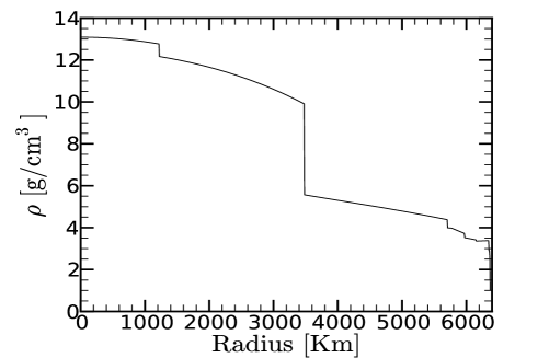
Figure 1: Earth matter density profile $\rho_{e}$   [g/cm³] as a function of radius.

The values of the total cross sections, for neutrino and antineutrino interaction with matter (nuclei) at high energies, have to be extrapolated from low energy data, since no measurements have been performed yet. In this work we use the cross sections reported in Ref.Gandhi:1998ri and present in Figs. 2 and 3 respectively for $\nu-N$ and ${\bar{\nu}}-N$. Comparison of the total cross sections $\nu-N$ and ${\bar{\nu}}-N$ shows that in the low energy limit $E_{\nu}\leq 10$ TeV there is a very small difference between these two which can be seen in Fig. 4.

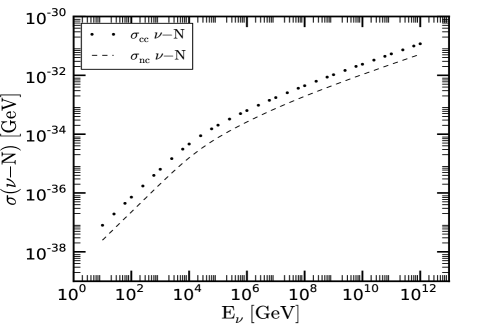
Figure 2: Neutrino-nucleon cross sections at high energies Gandhi:1998ri .

Figure 3: Antineutrino-nucleon cross sections ant high energies Gandhi:1998ri .

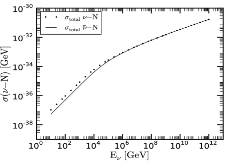
Figure 4: Comparison of both neutrino-nucleon and antineutrino-nucleon cross sections.

In Fig. 5,  $P_{shad}$ is plotted as a function of $E_{\nu}$, for a zenith angle $\theta=180^{\circ}$ (neutrinos arriving to the detector from underneath). From the graph it can be noticed that the shadowing factor decreases as the neutrino energy increases beyond $\sim 1$ TeV and the Earth becomes opaque for neutrinos with energies above $\sim 1000$ TeV. There is a small difference between neutrino and antineutrino shadowing factor above 1 TeV. Since we are interested in TeV neutrinos, the shadowing effect has to be taken into account properly in the calculation of neutrino fluxes arriving at the detector. Depending on the energy of the neutrinos, the interaction of the neutrinos with the medium inside the Earth will also result on flavor oscillations. Since in this work we will account for those neutrinos that go through the Earth before undergoing deep inelastic collision with the surround medium to the detector, we must take into account the flavor oscillation.

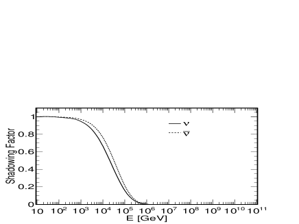
Figure 5: The shadowing factor $P_{shad}$ as a function of neutrino energy for a zenith angle $\theta=180^{\circ}$.

In Paper-I we have already used the analytic formalism developed by T. Ohlsson and H. Snellman (OS) to calculate three-flavor neutrino oscillationsOhlsson:1999xb ; Ohlsson:2001et in the presupernova starOliveros:2013apa and then calculate the flavor ratio of neutrinos arriving on Earth. Here we are extending the calculation by taking into account the matter effect of the Earth to calculate the flavor ratio at the IceCube detector. For this calculation we use the Earth density profile given in Eq. (4).

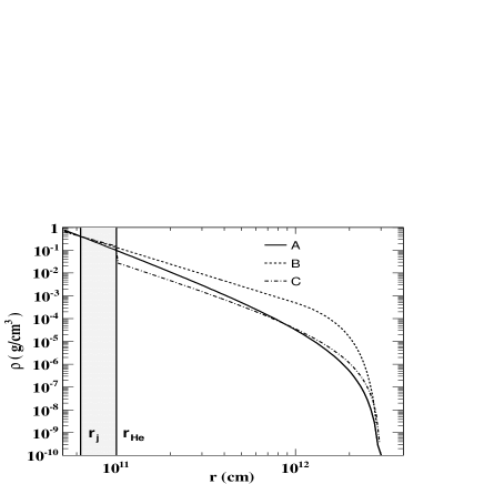
Figure 6: Density profiles of the progenitor star taken from Mena:2006eq . The density profiles [A], [B], [C] are described in detail in Oliveros:2013apa .

The input neutrino fluxes at the surface of the Earth, as functions of neutrino energy $E_{\nu}$, are those calculated in Paper-I, for three different models of the presupernova star, which we will refer to as model A, B and C and are discussed throughly in Paper-I. For reference we present the density profile of these three models in Fig. 6 and a detail description is given in paper-IOliveros:2013apa . In Figs. 7 and 8 the neutrino and antineutrino fluxes at the detector, as functions of neutrino energy, resulting from the models A and B (in (b), (c) and (d)) and taking into account the Earth’s matter effect, are compared with the case in which the effects of the stellar medium are ignored (in (a)). The two sets of plots, corresponding to different neutrino-mixing angles $\theta_{13}$, are shown. In these plots the neutrinos have traversed the whole Earth before arriving to the detector (a 180^∘ zenith angle). All other parameters are taken from the best fit parameters from different experiments which are surrarized in Table 1. We also consider two sets of parameters Set-I and Set-II corresponding to two different presuprenova star radii $R^{*}$ as shown in Table 1 and analyze our results.

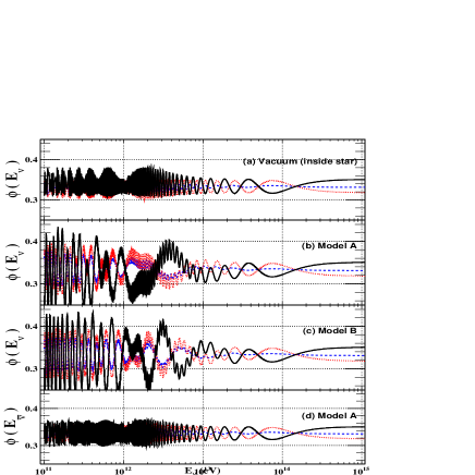
Figure 7: Neutrino and antineutrino fluxes at the detector. In (a), (b) and (c) solid lines is for $\Phi_{\nu_{e}}$, dashed lines are for $\Phi_{\nu_{\mu}}$, and dotted lines are for $\Phi_{\nu_{\tau}}$. In (d) solid line, dashed line and dotted line are for $\Phi_{\bar{\nu}_{e}}$, $\Phi_{\bar{\nu}_{\mu}}$ and $\Phi_{\bar{\nu}_{\tau}}$ respectively. The neutrino-mixing parameters are: $\delta_{CP}=0$; $\theta_{12}=33.8^{\circ}$; $\theta_{13}=8.8^{\circ}$; $\theta_{23}=45.0^{\circ}$; $\Delta m^{2}_{21}=8.0\times 10^{-5}$ eV²; $\Delta m^{2}_{23}=3.2\times 10^{-3}$ eV².

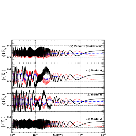
Figure 8: Same as Fig. 7 but here we consider $\theta_{13}=12.0^{\circ}$.

Table 1: We consider these parameters for our study. $R^{*}$ is the radius of the presupernova star. We consider three different values of $\Delta m^{2}_{32}$ to observe the variation in $R$.

Parameter	Set-I	Set-II
$R^{*}$	$3\times 10^{12}\,cm$	$2.7\times 10^{12}\,cm$
$\theta_{12}$	$33.8^{\circ}$	$33.8^{\circ}$
$\theta_{13}$	$8.8^{\circ}$	$12^{\circ}$
$\theta_{23}$	$45^{\circ}$	$45^{\circ}$
$\Delta m^{2}_{21}/eV^{2}$	$8.5\times 10^{-5}$	$8.5\times 10^{-5}$
$\Delta m^{2}_{32}/eV^{2}$	$1.4\times 10^{-3}$	$1.4\times 10^{-3}$
	$3.2\times 10^{-3}$	$3.2\times 10^{-3}$
	$6.0\times 10^{-3}$	$6.0\times 10^{-3}$

III Detection of neutrinos by IceCube

A neutrino detector, like IceCube, detect high energy neutrinos by observing the Cherenkov radiation emitted by the secondary charged particles produced when high energy neutrinos interact with the surrounding rock and iceicecubesite . These secondaries produce showers events and/or tracks events depending on the primary neutrino flavor. The neutrino interaction with rock and ice takes place through neutral current (NC) and/or charge current (CC) weak processes $\nu_{l}+N\rightarrow\nu_{l}({l})+X$. In the NC case, since there is a neutrino in the final state, the only signature of the interaction will be through the hadronic shower, independent of the neutrino flavor. In the CC case the end-result depends on neutrino flavor. If the interacting neutrino is an electron type, the resulting electron will quickly interact with the medium, producing an electromagnetic shower, which will overlap with the hadronic shower. If the neutrino is muon type, the resulting muon will produce a long track that emerges from the shower. Finally, if the neutrino is tau type, the resulting tau lepton may or may not produce a track depending on its energy. But when the tau decays into muon, $\tau\rightarrow\nu_{\mu}\,\mu\,\nu_{\tau}$ the later will produce a long track, just like in the case of a muon-neutrino CC interaction, this modifies the number of track events, which has to be accounted for. Since in this work we are considering neutrinos coming from underneath the detector, those with energies above 1 PeV will be drastically suppressed, and therefore the lollipop and double-bang events that are associated with very energetic $\nu_{\tau}$ will also be suppressedBeacom:2003nh . In this work we will not consider these kinds of events, however, we will include the $\mu$-track events induced by tau neutrinos, as explained above.

In conclusion, the ratio of track events to shower events is related in a convoluted way to the neutrino flavor ratios. However, given a set of flavor ratios, like 1:1:1 in the ”standard picture”, or any other set, like in the case we are presenting in this work, the ratio of tracks-to-showers R can be calculated. In the next section we discuss in detail the track-to-shower ratio calculation.

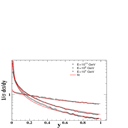
Figure 9: Comparison between our empirical fit, based on equation (14), and the Monte Carlo results presented in reference Bevan.:2007pt .

IV The track-to-shower ratio

The calculation of the track-to-shower ratio R presented in this section is based on the calculations from referencesBeacom:2003nh ; Esmaili:2009dz . Here we have included the shadowing effect due to the neutrino absorption by the Earth, $P_{shad}(E_{\nu},\theta)$. Since we are considering neutrinos coming from underneath, $\theta=180^{o}$, then $P_{shad}(E_{\nu})=P_{shad}(E_{\nu},\theta=180^{\text{o}})$. The ratio R is defined as:

$$\text{R}=\frac{\text{Number of}\ \mu\text{-track events}}{\text{Number of shower-like events}}.$$ (5)

The $\mu$-track events have two components: $N_{\mu\mu}$ from $\mu$-tracks induced by muon neutrinos, and $N_{\mu\tau}$ from $\mu$-tracks induced by tau neutrinos. The number of shower-like events have three components: $N_{sh_{had}}$ from hadronic showers associated with NC interaction, $N_{sh_{em}}$ from electromagnetic showers produced by CC interaction of $\nu_{e}$ and $N_{sh_{\tau}}$ from showers produced by CC interaction of $\nu_{\tau}$ decaying hadronically. So we can express $R$ as

$$\text{R}=\frac{N_{\mu\mu}+N_{\mu\tau}}{N_{sh_{had}}+N_{sh_{em}}+N_{sh_{\tau}}}.$$ (6)

The $\mu$-tracks induced by $\nu_{\mu}(\bar{\nu}_{\mu})$ result from the CC interaction of the neutrinos with the rock or the ice underground. The muons can travel a long distance before decaying; the effective muon range $R_{\mu}$ depends on the initial energy $E_{\mu}$ and the detection energy threshold $E_{\mu}^{th}$; in the case of IceCube this threshold is $\sim\,100$ GeV. The $\mu$-track induced by $\nu_{\tau}(\bar{\nu}_{\tau})$ result from the decay of a $\tau$ produced in a CC interaction into a $\mu$; this decay has a probability density $f(E_{\tau},E_{\mu})$ and a branching ratio $B=17.8\%$. The expressions for $N_{\mu\mu}$ and $N_{\mu\tau}$ are given by

$$N_{\mu\mu}=\rho AN_{A}\int_{E_{\mu}^{th}}^{\ \infty}\int_{E_{\mu}^{th}}^{E_{\nu_{\mu}}}R_{\mu}(E_{\mu},E_{\mu}^{th})P_{shad}(E_{\nu_{\mu}})\frac{dF_{\nu_{\mu}}}{dE_{\nu_{\mu}}}\frac{d\sigma^{CC}}{dE_{\mu}}dE_{\mu}dE_{\nu_{\mu}}\ \ +\ \ [\nu_{\mu}\rightarrow\bar{\nu}_{\mu}].$$ (7)

$$N_{\mu\tau} = B\rho AN_{A}\int_{E_{\mu}^{th}}^{\ \infty}\int_{E_{\mu}^{th}}^{E_{\nu_{\tau}}}\int_{E_{\mu}^{th}}^{\frac{E_{\tau}}{2}(1+\beta)}R_{\mu}(E_{\mu},E_{\mu}^{th})P_{shad}(E_{\nu_{\mu}})$$ (8)

$$\times\frac{dF_{\nu_{\tau}}}{dE_{\nu_{\tau}}}\frac{d\sigma^{CC}}{dE_{\tau}}f(E_{\tau},E_{\mu})dE_{\mu}dE_{\tau}dE_{\nu_{\tau}}\ \ +\ \ [\nu_{\tau}\rightarrow\bar{\nu}_{\tau}],$$

where the muon range is defined as

$$R_{\mu}(E_{\mu},E_{\mu}^{th})=(2.6\ \text{Km})\ln\left[\frac{2.0+4.2\times 10^{-3}E_{\mu}}{2.0+4.2\times 10^{-3}E_{\mu}^{th}}\right],$$ (9)

and its probability density is given by

$$f(E_{\tau},E_{\mu})\simeq\frac{5}{3E_{\tau}}-\frac{3E_{\mu}^{2}}{E_{\tau}^{3}}+\frac{4E_{\mu}^{3}}{3E_{\tau}^{4}}\ .$$ (10)

The expression for $f(E_{\tau},E_{\mu})$ is an approximation valid for $\beta\rightarrow 1\$ ($\gamma\gg 1$), where $\beta=\sqrt{1-1/\gamma^{2}\ }=\sqrt{1-(\frac{m_{\tau}}{E_{\tau}})^{2}\ }$. The number of shower-like events for the different kinds of processes are given by:

$$N_{sh_{had}}=\sum_{l=e,\mu,\tau}\rho ALN_{A}\left[\int_{E_{sh}^{th}}^{\ \infty}P_{shad}(E_{\nu_{l}})\frac{dF_{\nu_{l}}}{dE_{\nu_{l}}}\sigma^{NC}dE_{\nu_{l}}\ +\ \int_{E_{sh}^{th}}^{\ \infty}P_{shad}(E_{\bar{\nu}_{l}})\frac{dF_{\bar{\nu}_{l}}}{dE_{\bar{\nu}_{l}}}\sigma^{NC}dE_{\bar{\nu}_{l}}\right],$$ (11)

$$N_{sh_{em}}=\rho ALN_{A}\left[\int_{E_{sh}^{th}}^{\ \infty}P_{shad}(E_{\nu_{e}})\frac{dF_{\nu_{e}}}{dE_{\nu_{e}}}\sigma^{CC}dE_{\nu_{e}}\ +\ \int_{E_{sh}^{th}}^{\ \infty}P_{shad}(E_{\bar{\nu}_{e}})\frac{dF_{\bar{\nu}_{e}}}{dE_{\bar{\nu}_{e}}}\sigma^{CC}dE_{\bar{\nu}_{e}}\right],$$ (12)

$$N_{sh_{\tau}}=(1-B)\rho ALN_{A}\left[\int_{E_{sh}^{th}}^{\ \infty}P_{shad}(E_{\nu_{\tau}})\frac{dF_{\nu_{\tau}}}{dE_{\nu_{\tau}}}\sigma^{CC}dE_{\nu_{\tau}}\ +\ \int_{E_{sh}^{th}}^{\ \infty}P_{shad}(E_{\bar{\nu}_{\tau}})\frac{dF_{\bar{\nu}_{\tau}}}{dE_{\bar{\nu}_{\tau}}}\sigma^{CC}dE_{\bar{\nu}_{\tau}}\right],$$ (13)

where $\rho$ is the density of the detector medium, $A$ is the effective area of the detector, $L$ is the length of the detector, $N_{A}$ is the Avogadro’s number and $dF_{\nu_{l}}/dE_{\nu_{l}}$ is defined in Eq. (1). The normalization for this equation, $N_{\nu_{l}}$, is proportional to the neutrino flux, for the different flavors. Since $dF_{\nu_{l}}/dE_{\nu_{l}}$ is evaluated in the quotient of equation (5), the proportionality constant cancels out. The total cross sections for $CC$ ($\sigma^{CC}$) and $NC$ ($\sigma^{NC}$) shown in Figs. (2) and (3) are used to evaluate the $N_{sh_{had}}$ and $N_{sh_{em}}$.

In order to evaluate $d\sigma^{CC}/dE_{l}$ we performed an empirical fit to the differential cross section presented in Fig. 4 of reference Bevan.:2007pt , which is given as:

$$\frac{1}{\sigma^{CC}}\frac{d\sigma^{CC}}{dy}=N_{0}\left\{\begin{array}[]{lcc}b_{1}\ y^{-a_{1}}&\ \ \ \ \text{if}&\ y<y_{cut}\\ \\ b_{2}\ y^{-a_{2}}&\ \ \ \ \text{if}&\ y\geq y_{cut}\ ,\end{array}\right.$$ (14)

where $N_{0}$ is the normalization,

$$y=\frac{E_{\nu_{l}}-E_{l}}{E_{\nu_{l}}},$$ (15)

and

$$y_{cut}=\exp\left(\frac{\log b_{1}-\log b_{2}}{a_{1}-a_{2}}\right).$$ (16)

The parameters in Eq.(14) are as follows:

$$a_{1}=-0.0163\ x^{2}+0.3877\ x-1.1905,$$ (17)

$$a_{2}=-0.0222\ x^{2}+0.4222\ x-0.9833,$$ (18)

$$b_{1}=0.0168\ x^{2}-0.3683\ x+2.0038,$$ (19)

$$b_{2}=0.0139\ x^{2}-0.2739\ x+1.4233,$$ (20)

and

$$x=\log_{10}(E_{\nu_{l}}/\text{GeV}).$$ (21)

The normalization is set such that

$$\int_{0}^{1}\left(\frac{1}{\sigma^{CC}}\frac{d\sigma^{CC}}{dy}\right)dy=1\ .$$ (22)

We compare our fit with the data presented in referenceBevan.:2007pt which are shown in Fig. 9.

After performing the necessary change of variable from $E_{l}$ to $y$, one can evaluated the integrals numerically. The neutrino-flavor ratios, $R$, obtained after propagating the neutrinos from the source, all the way up to the detector, for different combinations of the parameters involved, and for different energies are used as input for the calculation.

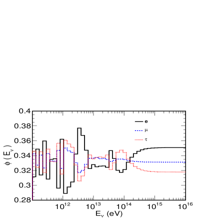
Figure 10: Neutrino flux $\Phi_{\nu}(E_{\nu})$ as a function of neutrino energy $E_{\nu}$ in the detector.

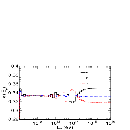
Figure 11: Antineutrino flux $\Phi(E_{\bar{\nu}})$ as a function of neutrino energy $E_{\nu}$ in the detector.

V Results

As can be seen from Figs.7 and 8, the normalized flux of neutrinos and antineutrinos in the detector depends on energy. For the calculation of the ratio $R$ we need the neutrino flux $dF_{\nu}/dE_{\nu}$. Neither we know the exact form of it nor the spectral index $\alpha$. But by considering the neutrino flux ratio 1:2:0 at the source, then propagating these neutrinos through the presupernova matter we calculated the normalized flux on the surface of the star in Paper-I. Here, we take these normalized flux and propagate the neutrinos through the distance between the source and the Earth, where Earth’s matter effect is included and calculate the normalized flux of these neutrinos and antineutrinos in the detector. For the calculation of the track-to-shower ratio $R$ of Eq.(5) we use these fluxes. But instead of calculating the flux for each energy, we divide the whole energy range to energy bins as $\Delta E_{\nu}=0.3E_{\nu}$ i.e. %30 energy resolution. Within each bin the flux is constant which we take by averaging the flux in the same energy bin. Here we have shown these avarage neutrino and antineutrino fluxes in Figs.10 and 11. From these figures, it is observed that the average neutrino and antineutrino fluxes are different for $E_{\nu}<2\times 10^{13}$ eV. Finally, we consider two values of the CP violating phase $\delta_{CP}=0$ and $\pi$ to see the change in $R$. The upper limit of the $E_{\nu}$ is taken to be $10$ PeV to evaluate the neutrino energy integrals. The following values are considered for the IceCube detector in our calculation: density of ice $\rho=0.051\,g\,cm^{-3}$, detector area $A=10^{10}\,cm^{2}$ and the detector length $L=10^{5}\,cm$. The results are presented in Figs. 12 to 20.

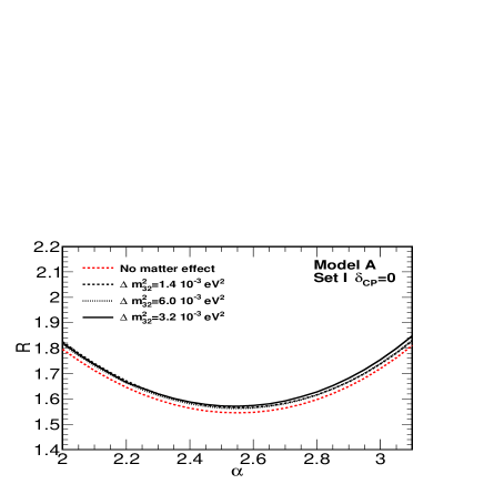
Figure 12: The track-to-shower ratio $R$ as a function of the spectral index $\alpha$ for $\delta_{CP}=0$ in Model-A.

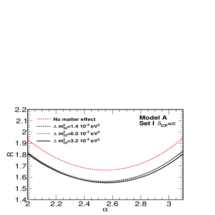
Figure 13: The track-to-shower ratio $R$ as a function of the spectral index $\alpha$ for $\delta_{CP}=\pi$ in Model A.

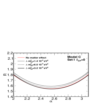
Figure 14: Same as Fig. 12 for model C.

Figure 15: Same as Fig. 13 for model C.

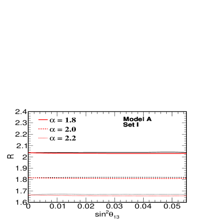
Figure 16: The track-to-shower ratio $R$ as a function of $sin^{2}\theta_{13}$ in Model-A for the parameter Set-I with $\Delta m^{2}_{32}=3.2\times 10^{-3}\,eV^{2}$. The black curve is for $\delta_{CP}=0$ and red one is for $\delta_{CP}=\pi$.

Figure 17: The track-to-shower ratio $R$ as a function of $sin^{2}\theta_{13}$ in Model-A for the parameter Set-II with $\Delta m^{2}_{32}=3.2\times 10^{-3}\,eV^{2}$. The black curve is for $\delta_{CP}=0$ and red one is for $\delta_{CP}=\pi$.

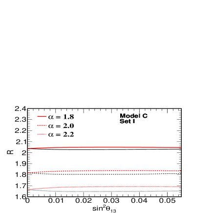
Figure 18: The track-to-shower ratio $R$ as a function of $sin^{2}\theta_{13}$ in Model-C for the parameter Set-I with $\Delta m^{2}_{32}=3.2\times 10^{-3}\,eV^{2}$. The black curve is for $\delta_{CP}=0$ and red one is for $\delta_{CP}=\pi$.

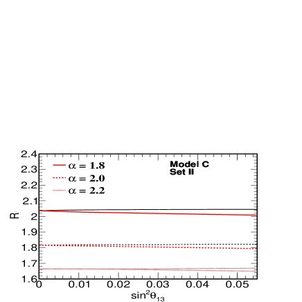
Figure 19: The track-to-shower ratio $R$ as a function of $sin^{2}\theta_{13}$ in Model-C for the parameter Set-II with $\Delta m^{2}_{32}=3.2\times 10^{-3}\,eV^{2}$. The black curve is for $\delta_{CP}=0$ and red one is for $\delta_{CP}=\pi$.

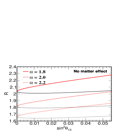
Figure 20: The track-to-shower ratio $R$ as a function of $sin^{2}\theta_{13}$ with no matter effect. Hre also the black curve is for $\delta_{CP}=0$ and red one is for $\delta_{CP}=\pi$. We take $\Delta m^{2}_{32}=3.2\times 10^{-3}\,eV^{2}$.

In Figs. 12 to 15, we have shown $R$ as a function of the spectral index $\alpha$ for models A and C. In these figures we also include no matter effect which implies: at the source we consider the flux ratio 1:2:0 and these neutrinos propagate up to the detector in vacuum. For our convenience we define the track-to-shower ratio for no matter effect as $R_{0}$. For $\delta_{CP}=0$ we found that $R_{0}\leq R$ for any given value of $\alpha$. Also the gap between $R$ and $R_{0}$ is small. On the other hand, for $\delta_{CP}=\pi$, always we found $R_{0}>R$ and the gap is bigger. The value of $R$ is minimum around $\alpha=2.6$ which is independent of whether we consider matter effect or not. We have also shown for three different $\Delta m^{2}_{32}$ values, which shows that there is very little variation in $R$. This minimum value of $R$ is also independent of $\Delta m^{2}_{32}$. The order in which $R$ is arranged for different $\Delta m^{2}_{32}$ values reverses by going from $\delta_{CP}=0$ to $\pi$, which can be seen by comparing Fig. 12 with Fig. 13 in model A and similarly Fig. 14 with Fig. 15 in model C. Here we have omitted the results from model B because the results are very similar to model A.

In Figs. 16 to 19 we have shown the variation of $R$ as a function of $sin^{2}{\theta_{13}}$ in models A and C for three different values of the spectral index $\alpha$. In these plots we observe that the ratio $R$ is almost constant for a given $\alpha$ and for both $\delta_{CP}=0$ and $\pi$, as we vary $sin^{2}{\theta_{13}}$ for all the models. Also the value of $R$ is higher for smaller $\alpha$.

We have also shown the $R$ as a function of $sin^{2}{\theta_{13}}$ for no matter effect in Fig.20. This shows a clear difference between $\delta_{CP}=0$ (lower curve) and $\delta_{CP}=\pi$ (upper curve) for each $\alpha$. These two curves diverge from the point $\theta_{13}=0$ as can be seen from the plots in Fig.20. Comparison of the matter effect (from Figs. 16 to 19) with the no matter effect Fig.20 shows that the $\delta_{CP}=\pi$ contribution is very much suppressed in matter compared to $\delta_{CP}=0$ contribution and makes them almost the same. This shows that the track-to-shower ratio $R$ for high energy neutrinos in IceCube is probably almost blind to CP violating phases when Earth matter effect is taken into account.

VI Summary

A very small fraction ($\leq\,10^{-3}$) of the core collapse supernovae can produce GRBs by launching a successful jet. Although the majority of these core collapse can not produce GRBs, very high energy neutrinos can easily be produced in their choked jets. These neutrinos propagating through the over burden matter can undergo oscillation and the flux ratio on the surface of the star can be different from the point where these neutrinos were produced. The Mpc long baseline, from the surface of the star to the surface of the Earth, these neutrinos will have vacuum oscillation. Before reaching to the detector from the opposite side of the Earth, these neutrinos will cross the dimeter of the Earth and can undergo again matter oscillation. By considering the realistic density profile of the Earth we have extended our previous work to study numerically the three neutrino oscillation and evaluate the change in the flux ratio in the detector. Depending on the energy of these neutrinos, there can also be shadowing effect and neutrinos above few PeV can be completely absorbed. In this work we have done a through analysis of the high energy neutrino propagation in the Earth before reaching to the detector by taking into account the shadowing effect. The track-to-shower ratio $R$ is calculated for these high energy neutrinos. In the calculation of $R$ we have included the shadowing effect and the contribution of muon track produced by the high energy $\tau$ lepton decay around the IceCube detector. These $\tau$ leptons are produced due to the CC interaction of $\nu_{\tau}$ with the surround rock and ice of the detector. We have studied the variation of $R$ when the spectral index $\alpha$ and the mixing angle $sin^{2}\theta_{13}$ vary. We found that $R$ has a minimum around $\alpha=2.6$ and is independent of whether we consider matter effect or not. This minimum value of $R$ is also independent of $\Delta m^{2}_{32}$ value. We observed that the ratio $R$ is different for $\delta_{CP}=0$ and $\pi$ when no matter effect is considered. But when Earth matter contribution is taken into account, the $R$ value is almost blind to these different CP phases.

S.S. is thankful to Departamento de Fisica de Universidad de los Andes, Bogota, Colombia, for their kind hospitality during his several visits. This work is partially supported by DGAPA-UNAM (Mexico) Project No. IN103812.

References

- (1)
- (2) B. Zhang and P. Meszaros, Int. J. Mod. Phys. A 19, 2385 (2004) [astro-ph/0311321].
- (3) C. Kouveliotou, C. A. Meegan, G. J. Fishman, N. P. Bhyat, M. S. Briggs, T. M. Koshut, W. S. Paciesas and G. N. Pendleton, Astrophys. J. 413, L101 (1993).
- (4) E. Waxman and J. N. Bahcall, Phys. Rev. Lett. 78, 2292 (1997).
- (5) E. Waxman and J. N. Bahcall, Phys. Rev. D 59, 023002 (1999).
- (6) E. Berger, S. R. Kulkarni, D. A. Frail and A. M. Soderberg, Astrophys. J. 599, 408 (2003).
- (7) S. E. Woosley and J. S. Bloom, Ann. Rev. Astron. Astrophys. 44, 507 (2006) [astro-ph/0609142].
- (8) P. A. Mazzali, J. S. Deng, N. Tominaga, K. Maeda, K. .Nomoto, T. Matheson, K. S. Kawabata and K. Z. Stanek et al., Astrophys. J. 599, L95 (2003) [astro-ph/0309555].
- (9) S. Sahu and B. Zhang, Res. Astron. Astrophys. 10, 943 (2010) [arXiv:1007.4582 [hep-ph]].
- (10) A. F. Osorio Oliveros , S. Sahu and J. C. Sanabria, Eur. Phys. J. C 73, 2574 (2013). [astro-ph/1304.4906].
- (11) M. G. Aartsen et al. [IceCube Collaboration], Phys. Rev. Lett. 111, 021103 (2013) [arXiv:1304.5356 [astro-ph.HE]].
- (12) M. G. Aartsen et al. [IceCube Collaboration], Science 342, no. 6161, 1242856 (2013) [arXiv:1311.5238 [astro-ph.HE]].
- (13) M. G. Aartsen et al. [IceCube Collaboration], arXiv:1405.5303 [astro-ph.HE].
- (14) M. G. Aartsen et al. [IceCube Collaboration], arXiv:1410.1749 [astro-ph.HE].
- (15) F. Halzen and D. W. Hooper, Astrophys. J. 527, L93 (1999) [astro-ph/9908138].
- (16) J. K. Becker, Phys. Rept. 458, 173 (2008) [arXiv:0710.1557 [astro-ph]].
- (17) R. Gandhi, C. Quigg, M. H. Reno and I. Sarcevic, Phys. Rev. D 58, 093009 (1998) [hep-ph/9807264].
- (18) O. Mena, I. Mocioiu and S. Razzaque, Phys. Rev. D 75, 063003 (2007) [astro-ph/0612325].
- (19) T. Ohlsson and H. Snellman, J. Math. Phys. 41, 2768 (2000) [Erratum-ibid. 42, 2345 (2001)] [hep-ph/9910546].
- (20) T. Ohlsson and H. Snellman, Eur. Phys. J. C 20, 507 (2001) [hep-ph/0103252].
- (21) See IceCube website: http://icecube.wisc.edu/
- (22) J. F. Beacom, N. F. Bell, D. Hooper, S. Pakvasa and T. J. Weiler, Phys. Rev. D 68, 093005 (2003) [Erratum-ibid. D 72, 019901 (2005)] [hep-ph/0307025].
- (23) A. Esmaili and Y. Farzan, Nucl. Phys. B 821, 197 (2009) [arXiv:0905.0259 [hep-ph]].
- (24) S. Bevan., S. Danaher., J. Perkin., S. Ralph., C. Rhodes., L. Thompson., T. Sloan. and D. Waters., Astropart. Phys. 28, 366 (2007) [arXiv:0704.1025 [astro-ph]].