Guaranteed Matrix Completion via Non-convex Factorization

Abstract

Matrix factorization is a popular approach for large-scale matrix completion. The optimization formulation based on matrix factorization can be solved very efficiently by standard algorithms in practice. However, due to the non-convexity caused by the factorization model, there is a limited theoretical understanding of this formulation. In this paper, we establish a theoretical guarantee for the factorization formulation to correctly recover the underlying low-rank matrix. In particular, we show that under similar conditions to those in previous works, many standard optimization algorithms converge to the global optima of a factorization formulation, and recover the true low-rank matrix. We study the local geometry of a properly regularized factorization formulation and prove that any stationary point in a certain local region is globally optimal. A major difference of our work from the existing results is that we do not need resampling in either the algorithm or its analysis. Compared to other works on nonconvex optimization, one extra difficulty lies in analyzing nonconvex constrained optimization when the constraint (or the corresponding regularizer) is not “consistent” with the gradient direction. One technical contribution is the perturbation analysis for non-symmetric matrix factorization.

1 Introduction

In the era of big data, there has been an increasing need for handling the enormous amount of data generated by mobile devices, sensors, online merchants, social networks, etc. Exploiting low-rank structure of the data matrix is a powerful method to deal with “big data”. One prototype example is the low rank matrix completion problem in which the goal is to recover an unknown low rank matrix $M\in\mathbb{R}^{m\times n}$ for which only a subset of its entries $M_{ij},(i,j)\in\Omega\subseteq\{1,2,\dots,m\}\times\{1,2,\dots,n\}$ are specified. Matrix completion has found numerous applications in various fields such as recommender systems [1], computer vision [2] and system identification [3], to name a few.

There are two popular approaches to impose the low-rank structure: the nuclear norm based approach and the matrix factorization (MF) based approach. In the first approach, the whole matrix is the optimization variable and the nuclear norm (denoted as $\|\cdot\|_{*}$) of this matrix variable, which can be viewed as a convex approximation of its rank, serves as the objective function or a regularization term. For the matrix completion problem, the nuclear norm based formulation becomes either a linearly constrained minimization problem [4]

$$\min_{Z\in\mathbb{R}^{m\times n}}\quad\|Z\|_{*},\quad{\rm s.t.}\quad Z_{ij}=M_{ij},\ \forall\ (i,j)\in\Omega,$$ (1)

a quadratically constrained minimization problem

$$\min_{Z\in\mathbb{R}^{m\times n}}\quad\|Z\|_{*},\quad{\rm s.t.}\sum_{(i,j)\in\Omega}(Z_{ij}-M_{ij})^{2}\leq\epsilon,$$ (2)

or a regularized unconstrained problem

$$\min_{Z\in\mathbb{R}^{m\times n}}\quad\|Z\|_{*}+\lambda\sum_{(i,j)\in\Omega}(Z_{ij}-M_{ij})^{2}.$$ (3)

On the theoretical side, it has been shown that given a rank-$r$ matrix $M$ satisfying an incoherence condition, solving (1) will exactly reconstruct $M$ with high probability provided that $O(r(m+n)\log^{2}(m+n))$ entries are uniformly randomly revealed [4, 5, 6, 7]. This result was later generalized to noisy matrix completion, whereby the optimization formulation (2) is adopted [8]. Using a different proof framework, reference [9] provided theoretical guarantee for a variant of the formulation (3). On the computational side, problems (1) and (2) can be reformulated as a semidefinite program (SDP) and solved to global optima by standard SDP solvers when the matrix dimension is smaller than 500. To solve problems with larger size, researchers have developed first order algorithms, including the SVT (singular value thresholding) algorithm for the formulation (1) [10], and several variants of the proximal gradient method for the formulation (3) [11, 12] . Although linear convergence of the proximal gradient method has been established for the formulation (3) under certain conditions [13, 14], the per-iteration cost of computing SVD (Singular Value Decomposition) may increase rapidly as the dimension of the problem increases, making these algorithms rather slow or even useless for problems of huge size. The other major drawback is the memory requirement of storing a large $m$ by $n$ matrix.

In the second approach, the unknown rank $r$ matrix is expressed as the product of two much smaller matrices $XY^{T}$, where $X\in\mathbb{R}^{m\times r},Y\in\mathbb{R}^{n\times r}$, so that the low-rank requirement is automatically fulfilled. Such a matrix factorization model has long been used in PCA (principle component analysis) and many other applications [15]. It has gained great popularity in the recommender systems field and served as the basic building block of many competing algorithms for the Netflix Prize [1, 16] due to several reasons. First, the compact representation of the unknown matrix greatly reduces the per-iteration computation cost as well as the storage space (requiring essentially linear storage of $O((m+n)r)$ for small $r$). Second, the per-iteration computation cost is rather small and people have found in practice that huge size optimization problems based on the factorization model can be solved very fast. Third, as elaborated in [1], the factorization model can be easily modified to incorporate additional application-specific requirements.

A popular factorization based formulation for matrix completion takes the form of an unconstrained regularized square-loss minimization problem [1]:

$$\begin{split}\mathrm{P}0:\quad\min_{X\in\mathbb{R}^{m\times r},Y\in\mathbb{R}^{n\times r}}\quad&\frac{1}{2}\sum_{(i,j)\in\Omega}[M_{ij}-(XY^{T})_{ij}]^{2}+\lambda(\|X\|_{F}^{2}+\|Y\|_{F}^{2}).\end{split}$$ (4)

There are a few variants of this formulation: the coefficient $\lambda$ can be zero [17, 18, 19, 20] or different for each row of $X,Y$ [21]; each square loss term $[M_{ij}-(XY^{T})_{ij}]^{2}$ can have different weights [1]; an additional matrix variable $Z\in\mathbb{R}^{n\times r}$ can be introduced [22]. Problem (4) is a non-convex fourth-order polynomial optimization problem, and can be solved to stationary points by standard nonlinear optimization algorithms such as gradient descent method, alternating minimization [1, 21, 18, 19] and SGD (stochastic gradient descent) [23, 24, 16, 1]. Alternating minimization is easily parallelizable but has higher per-iteration computation cost than SGD; in contrast, SGD requires little computation per iteration, but its parallelization is challenging. Recently several parallelizable variants of the SGD [25, 26, 27] and variants of the block coordinate descent method with very low per-iteration cost [28, 29] have been developed. Some of these algorithms have been tested in distributed computation platforms and can achieve good performance and high efficiency, solving very large problems with more than a million rows and columns in just a few minutes.

1.1 Our contributions

Despite the great empirical success, the theoretical understanding of the algorithms for the factorization based formulation is fairly limited. More specifically, the fundamental question of whether these algorithms (including many recently proposed ones) can recover the true low-rank matrix remains largely open. In this paper, we partially answer this question by showing that under similar conditions to those used in previous works, many standard optimization algorithms for a factorization based formulation (see (18)) indeed converge to the true low-rank matrix (see Theorem 3.1). Our result applies to a large class of algorithms including gradient descent, SGD and many block coordinate descent type methods such as two-block alternating minimization and block coordinate gradient descent. We also show the linear convergence of some of these algorithms (see Theorem 3.2 and Corollary 3.2).

To the best of our knowledge, our result is the first one that analyzes the geometry of matrix factorization in Euclidean space for matrix completion. In addition, our result also provides the first recovery guarantee for alternating minimization without resampling (i.e. without using independent samples in different iterations). Below we elaborate these two contributions in light of the existing works.

1) We analyze the local geometry of the matrix factorization formation (in Euclidean space). We argue that the success of many algorithms attributes mostly (or at least partially) to the geometry of the problem, rather than the specific algorithms being used. The geometrical property we establish is that the local gradient direction $-\nabla f(x)$ is aligned with the global descent direction $x^{*}-x$. For the classical matrix factorization formulation $\|M-XY^{T}\|_{F}^{2}$, we develop a novel perturbation analysis to deal with the ambiguity of the factorization. For the sampling loss $\|\mathcal{P}_{\Omega}(M-XY^{T})\|_{F}^{2}$, an incoherence regularizer (or constraint) is needed, which causes an extra difficulty of analyzing nonconvex constrained optimization. Unfortunately, projection to the constraint (or the gradient of the regularizer) is not aligned with the global direction, and we add one more regularizer to “correct” the local descent direction. A high-level lesson is that regularization may change the geometry of the problem.

2) Our result applies to the standard forms of the algorithms (though our optimization formulation is a bit different), which do not require the additional resampling scheme used in other works [17, 18, 19, 20]. We obtain a sample complexity bound that is independent of the recovery error $\epsilon$, while all previous sample complexity bounds for the matrix factorization based formulation (in Euclidean space) depend on $\epsilon$. There is a subtle theoretical issue for the resampling scheme; see more discussions in Section 1.2 and [30, Sec. 1.5.3].

1.2 Related works

Factorization models. The first recovery guarantee for the factorization based matrix completion is provided in [31], where Keshavan, Montanari and Oh considered a factorization model in Grassmannian manifold and showed that the matrix can be recovered by a proper initialization and a gradient descent method on Grassmannian manifold. Besides being quite complicated, this model is not as flexible as the factorization model in Euclidean space, and it is not easy to solve by many advanced large-scale optimization algorithms. Moreover, most algorithms in Grassmann manifold require line search, and little is known about the convergence rate.

The factorization model in Euclidean space was first analyzed in an unpublished work [17] of Keshavan , as well as a later work of Jain et al. [18]. Both works considered alternating minimization with resampling scheme, a special variant of the original alternating minimization. The sample complexity bounds were later improved by Hardt [19] and Hardt and Wooters [20], where in the latter work, notably, the authors devised an algorithm with a corresponding sample complexity bound independent of the condition number. However, these improvements are obtained for more sophisticated versions of resampling-based alternating minimization, not the typical alternating minimization algorithm.

Resampling. The issues of resampling have been discussed in a recent work on phase retrieval by Candès et al.[32]. We will point out a subtle theoretical issue not mentioned in [32], as well as some other practical issues.

The resampling scheme (a.k.a. golfing scheme [6]) can be used at almost no cost for the nuclear norm approach [33, 6, 7], but for the alternating minimization it causes many issues. At first, it may seem that for both approaches resampling is a cheap way to get around a common difficulty: the dependency of the iterates on the sample set. However, there is a crucial difference: for the nuclear norm approach, resampling is just a proof technique used in a “conceptual” algorithm for constructing the dual certificate, while for the alternating minimization, resampling is used in the actual algorithm. This difference causes some issues of resampling-based alternating minimization at conceptual, practical and theoretical levels.

1) Gap between theory and algorithm. Algorithmically, an easy resampling scheme is to randomly partition the given set $\Omega$ into non-overlapping subsets $\Omega_{k},k=1,\dots,L$, as proposed in [17, 18] . However, the results in [17, 18, 19, 20] actually require a generative model of independent $\Omega_{k}$’s, instead of sampling $\Omega_{k}$’s based on a given $\Omega$. Therefore, the results in [17, 18, 19, 20] do not directly apply to the partition based resampling scheme that is easy to use. See [30, Sec. 1.5.3] for more discussions on this subtle issue.

This issue has been discussed by Hardt and Wooters in [20, Appendix D], and they proposed a new resampling scheme [20, Algorithm 6] to which the results in [17, 18, 19, 20] can apply, provided that the generative model of $\Omega$ is exactly known. In practice, the underlying generative model of $\Omega$ is usually unknown, in which case the scheme [20, Algorithm 6] does not work. In contrast, the classical results in [4, 5, 7, 6] and our result herein are robust to the generative model of $\Omega$: these results actually state that for an overwhelming portion of $\Omega$ with a given size, one can recover $M$ through a certain algorithm, thus for many reasonable probability distributions of $\Omega$ a high probability result holds.

2) Impracticality. As argued previously, assuming a generative model of $\Omega_{k}$’s is not practical since $\Omega$ is usually given. For given $\Omega$, the only known validated resampling scheme [20, Algorithm 6], besides not being robust to the underlying generative model of $\Omega$, might be a bit complicated to use in practice. Even the simple resampling scheme of partitioning $\Omega$ (which has not been validated yet) is rather unrealistic since each sample is used only once during the algorithm.

3) Inexact recovery. A theoretical consequence of the resampling scheme is that the required sample complexity $|\Omega|$ becomes dependent on the desired accuracy $\epsilon$, and goes to infinity as $\epsilon$ goes to zero. This is different from the classical results (and ours) where exact reconstruction only requires finite samples. While it is common to see the dependency of time complexity on the accuracy $\epsilon$, it is relatively uncommon to see the dependency of sample complexity on $\epsilon$.

In a recent work [34] the authors have managed to remove the dependency of the required sample size on $\epsilon$ by using a singular value projection algorithm. However, [34] considers a matrix variable of the same size as the original matrix, which requires significantly more memory than the matrix factorization approach considered in this paper. Moreover, it requires resampling at a number of iterations (though not all), which may suffer from the same issues we mentioned earlier. The resampling is also required in the recent work of [35]; see [30, Sec. 1.5.3] for more discussions.

Other works on non-convex formulations. Non-convex formulation has also been studied for the phase retrieval problem in some recent works [36, 32]. These works provide theoretical guarantee for some algorithms specially tailored to certain non-convex formulations and with specific initializations. The major difference between [36] and [32] is that the former requires independent samples in each iteration, while the latter uses the same samples throughout in the proposed algorithm. As mentioned earlier, such a difference also exists between all previous works on alternating minimization for matrix completion [17, 18, 19, 20] and our work.

Finally, we note that there is a growing list of works on the theoretical guarantee of non-convex formulations for various problems, such as sparse regression (e.g. [37, 38, 39]), sparse PCA [40, 41], robust PCA [42] and EM (Expected-Maximization) algorithm [43, 44]. We emphasize several aspects that distinguish our paper from other recent works on non-convex optimization. First, our paper is one of the first to analyze the (local) geometry of the problem. Second, we deal with non-symmetric matrix factorization which has a more bizarre geometry than symmetric matrix factorization and some other models. Third, one difficulty of our problem essentially lies in nonconvex constrained optimization (though we consider the closely related regularized form).

1.3 Proof Overview and Techniques

Basic idea: local geometry. The very first question is what kind of property can ensure global convergence for non-convex optimization. We will establish a local geometrical property of a regularized objective such that any stationary point in a local region is globally optimal. This is achieved in three steps: (i) study the local geometry of the fully observed objective $\|M-XY^{T}\|_{F}^{2}$; (ii) study the local geometry of the matrix completion objective $\|\mathcal{P}_{\Omega}(M-XY^{T})\|_{F}^{2}$; (iii) study the local geometry of a regularized objective. Next, we will discuss the difficulties involved in each step and describe how we address these difficulties.

Local geometry of $\|M-XY^{T}\|_{F}^{2}$. We start by considering a simple case that $M$ is fully observed and the objective function is $f(X,Y)=\|M-XY^{T}\|_{F}^{2}$. What is the geometrical landscape of this function? In the simplest case $m=n=r=1$ and $f(x,y)=(xy-1)^{2}$, the set of stationary points is $\{(x,y)\mid xy=1\}\cup\{(0,0)\}$, in which $(0,0)$ is a saddle point and the curve $xy=1$ consists of global optima. We plot the function around the curve $xy=1$ in the positive orthant in Figure 1.

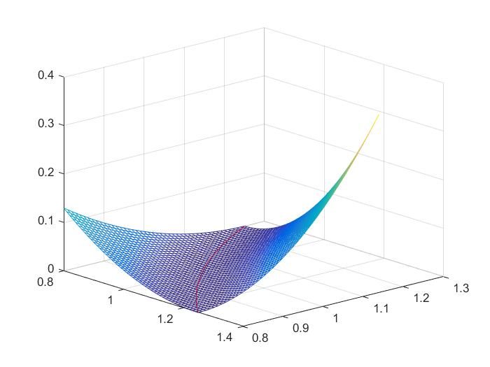
Figure 1: The plot of function $f(x,y)=(xy-1)^{2}$ around the set of global optima $xy=1$ in the positive orthant. The bottom of this bowl shape is a hyperbola $xy=1$.

Clearly a certain geometrical property prevents bad local minima in the neighborhood of the global optima, but what kind of property? We emphasize that the property can not be local convexity because the set of global optima is non-convex in $\mathbb{R}^{2}$. Due to the intrinsic symmetry that $f(x,y)=f(xq,yq^{-1})$, only the product $z=xy$ affects the value of $f$. We hope that the strong convexity of $(1-z)^{2}$ can be partially preserved when $z$ is reparameterized into $z=xy$. It turns out we can prove the following local convexity-type property: for any $(x,y)$ such that $xy$ is close to $1$ and $|x|,|y|$ are upper bounded, there exists $uv=1$ such that

$$\langle\nabla f(x,y),(x,y)-(u,v)\rangle\geq c\|(x,y)-(u,v)\|^{2}.$$

An interpretation is that the negative gradient direction $-\nabla f$ should be aligned with the global direction $(u,v)-(x,y)$; a convex function has a similar property, but the difference is that here the global direction is adjusted according to the position of $(x,y)$.

For general $m,n,r$, the geometrical landscape is probably much more complicated than the scalar case. Nevertheless, we can still prove that the convexity of $\|M-Z\|^{2}$ is partially preserved when reparameterizing $Z$ as $Z=XY$. The exact expression is a variant of (6) which we will discuss in more detail later. Technically, we need to connect the Euclidean space and the quotient manifold via “coupled perturbation analysis”: given $X,Y$ such that $\|XY^{T}-M\|_{F}$ is small, find decomposition $M=UV^{T}$ such that $U,V$ are close to $X$ and $Y$ respectively (a simpler version of Proposition 4.1). The difference from traditional perturbation analysis of Wedin [45] (i.e. if two matrices are close then their row/column spaces are close) is that in [45] the row/column spaces are fixed while in our problem $U,V$ are up to our choice.

Local geometry of $\|\mathcal{P}_{\Omega}(M-XY^{T})\|_{F}^{2}$. Let us come back to the original matrix completion problem, in which an additional sampling operator $\mathcal{P}_{\Omega}$ is introduced. Similarly, we hope that $f_{\Omega}(Z)=\frac{1}{2}\|\mathcal{P}_{\Omega}(M-Z)\|^{2}$ is strongly convex and this strong convexity can be partially preserved after reparametrization $Z=XY^{T}$. However, one issue is that the function $f_{\Omega}(Z)$ is possibly non-strongly-convex (though still convex). In fact, if $f_{\Omega}$ is locally strongly convex around $M$, then we should have

$$f_{\Omega}(Z)-f_{\Omega}(M)\geq O(\|Z-M\|_{F}^{2}),\forall\ Z\text{ close to }M.$$

Assuming $Z$ is rank-$r$, this inequality can be rewritten as

$$\|\mathcal{P}_{\Omega}(M-XY^{T})\|_{F}^{2}\geq Cp\|M-XY^{T}\|_{F}^{2},\ \forall(X,Y)\in K(\delta),$$ (5)

where $K(\delta)$ is a neighborhood of $M$ defined as $\{(X,Y)\mid\|XY^{T}-M\|_{F}\leq\delta\}$ and $C$ is a numerical constant. We wish (5) to hold with high probability (w.h.p.) for random $\Omega$ in which each position in $M$ is chosen with probability $p$. This inequality is closely related to matrix RIP (restricted isometry property) in [8] (see equation (III.4) therein). If $X,Y$ are independent of $\Omega$, then (5) follows easily from the concentration inequalities. Unfortunately, if $X,Y$ are chosen arbitrarily instead of independently from $\Omega$, the bound (5) may fail to hold.

A solution, as employed in [31], is to utilize a random graph lemma in [46] which provides a bound on $\|\mathcal{P}_{\Omega}(A)\|_{F}$ for any rank-$1$ matrix $A$ (possibly dependent on $\Omega$). This lemma, combined with another probability result in [4], implies a bound on $\|\mathcal{P}_{\Omega}(M-XY^{T})\|_{F}$. However, this bound is not good enough since it only leads to (5) when $\delta=O(1/n)$. The underlying reason is that the bound given by the random graph lemma is actually quite loose if $X$ or $Y$ have unbalanced rows, i.e. certain row has large norm. One solution is to force the iterates to have bounded row norms (a.k.a. incoherent), by adding a constraint or regularizer. With the incoherence requirement on $X,Y$, now (5) can be shown to be hold for $\delta=O(1)$, or more precisely, $\delta=O(\Sigma_{\min})$, where $\Sigma_{\min}$ is the minimum eigenvalue of $M$. With such a $\delta$, it is possible to find an initial point in the region $K(\delta)$.

In summary, although $f_{\Omega}(Z)=\frac{1}{2}\|\mathcal{P}_{\Omega}(Z-M)\|_{F}^{2}$ is possibly non-strongly-convex, by restricting to an incoherent neighborhood of $M$ it is “relative” strongly convex (called “relative” since we fix $M$ in (5)). More specifically, we have that w.h.p.

$$\|\mathcal{P}_{\Omega}(M-XY^{T})\|_{F}^{2}\geq Cp\|M-XY^{T}\|_{F}^{2},\ \forall(X,Y)\in\mathcal{B}\triangleq K(\delta)\cap K_{1}.$$ (6)

where $K_{1}$ denotes the set of $(X,Y)$ with bounded row norms. Note that this inequality also implies that global optimally in $\mathcal{B}$ leads to exact recovery; or equivalently, zero training error leads to zero generalization error.

Having established the geometry of $f_{\Omega}(Z)$, we can use the same technique for the fully observed case to show the local geometry of

$$F(X,Y)\triangleq f_{\Omega}(X,Y)=\frac{1}{2}\|\mathcal{P}_{\Omega}(M-XY^{T})\|_{F}^{2}.$$

More specifically, we can prove that for any $(X,Y)\in\mathcal{B}$, there exists $(U,V)\in\mathcal{X}^{*}=\{(U,V)\in\mathbb{R}^{m\times r}\times\mathbb{R}^{n\times r}\mid UV^{T}=M\}$ such that

$$\langle\nabla_{X}F(X,Y),X-U\rangle+\langle\nabla_{Y}F(X,Y),Y-V\rangle\geq c(\|X-U\|_{F}^{2}+\|Y-V\|_{F}^{2}).$$ (7)

Denoting $\bm{x}=(X,Y),\bm{x}^{*}=(U,V)$ and utilizing $\nabla F(\bm{x}^{*})=0$, (7) becomes

$$\forall\ \bm{x}\in\mathcal{B},\ \exists\ \bm{x}^{*}\in\mathcal{X}^{*},\ \text{ s.t.}\ \langle\nabla F(\bm{x})-\nabla F(\bm{x}^{*}),\bm{x}-\bm{x}^{*}\rangle\geq c\|\bm{x}-\bm{x}^{*}\|^{2}.$$ (8)

It links the local optimality measure $\|\nabla F(\bm{x})\|$ with the global optimality measure $\text{dist}(\bm{x},\mathcal{X}^{*})=\min_{\bm{x}^{*}\in\mathcal{X}^{*}}\|\bm{x}-\bm{x}^{*}\|$, and implies that any stationary point of $F$ in $\mathcal{B}$ is a global minimum.

If (8) holds for arbitrary $\bm{x},\bm{x}^{*}$ then $F$ would be strongly convex in $\bm{x}$. Let us emphasize again two differences of (8) with local strong convexity: i) since $\bm{x}^{*}$ is not arbitrary but has to be one global minimum, (8) indicates local “relative convexity” of $F$; ii) due to the ambiguity of factorization, $\bm{x}^{*}$ should be chosen according to $\bm{x}$, thus (8) indicates local relative convexity up to a group transformation (it might be conceptually helpful to view it as a property in the quotient manifold, but we do not explicitly exploit its structure).

Local geometry with regularizers/constraints. The property (8) is still not desirable. The original purpose of studying geometry is to show there is no spurious “1st order local-min” (point that satisfies 1st order optimality conditions). To establish the geometrical property with sampling, we restrict to an incoherent set $K_{1}$, but this restriction changes the meaning of the 1st order local-min. In fact, to ensure the iterates stay in the incoherent region $K_{1}$, we need to solve a constrained optimization problem $\min_{\bm{x}\in K_{1}}F(\bm{x})$ or a regularized problem $\min_{\bm{x}}F(\bm{x})+G_{1}(\bm{x})$ where $G_{1}$ is a regularizer forcing $\bm{x}$ to be in $K_{1}$. Standard optimization algorithms converge to the KKT points of $\min_{\bm{x}\in K_{1}}F(\bm{x})$ or the stationary points of $F+G_{1}$, which may not be the stationary points of $F$. The property (8) only implies any stationary point of $F$ in $\mathcal{B}$ is globally optimal.

We shall focus on the regularized problem $\min F+G_{1}$; the constrained problem $\min_{\bm{x}\in K_{1}}F$ is similar. Because of the extra regularizer, the property (8) is not enough. We need to prove a result similar to (8), but with $\nabla F$ replaced by $\nabla F+\nabla G_{1}$:

$$\forall\ \bm{x}\in\mathcal{B},\ \exists\ \bm{x}^{*}\in\mathcal{X}^{*},\ \text{s.t.}\ \langle\nabla F(\bm{x})+\nabla G_{1}(\bm{x}),\bm{x}-\bm{x}^{*}\rangle\geq c\|\bm{x}-\bm{x}^{*}\|^{2}.$$ (9)

If it happens to be the case that

$$\langle\nabla G_{1}(\bm{x}),\bm{x}-\bm{x}^{*}\rangle\geq 0,$$ (10)

then combining with the existing result (8) we are done; unfortunately, we do not know how to prove (10). Intuitively, (10) means that $-\nabla G_{1}(\bm{x})$, which is almost the same direction as the projection to the incoherent region $K_{1}$, is positively correlated with the global direction $\bm{x}^{*}-\bm{x}$. At first sight, this seems trivially true because for any point $\bar{\bm{x}}\in K_{1}$ we have $\langle\nabla G_{1}(\bm{x}),\bm{x}-\bar{\bm{x}}\rangle\geq 0$ (as illutrated in Fig. 2). However, a rather strange issue is that $\bm{x}^{*}$ is chosen to be a point in $\{(U,V)\mid UV^{T}=M\}$ that is close to $\bm{x}$, thus there is no guarantee that $\bm{x}^{*}$ lies in $K_{1}$. An underlying reason is that the global optimum set $\{(U,V)\mid UV^{T}=M\}$ is unbounded and thus not a subset of $K_{1}$. If we enforce $(U,V)$ to be in $K_{1}$, we may not be able to find $(U,V)$ that is close enough to $(X,Y)$.

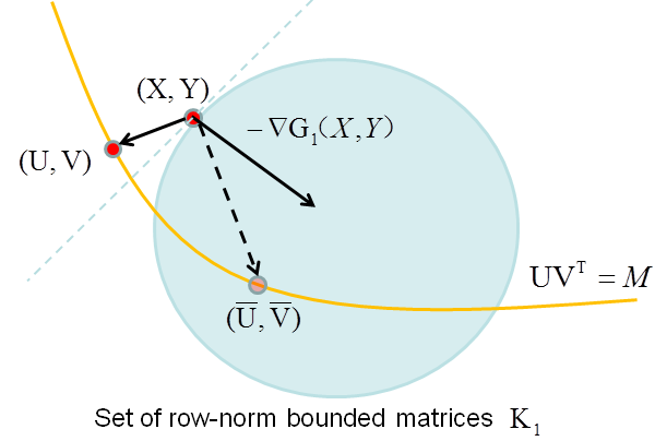
Figure 2: Illustration of why a single regularizer $G_{1}$ is not enough. The requirement (10) means $-\nabla G_{1}(\bm{x})=-\nabla G_{1}(X,Y)$ is positively correlated with $\bm{x}^{*}-\bm{x}$. This holds if we could pick some $\bm{x}^{*}=(\bar{U},\bar{V})$ lying in the row-bounded region $K_{1}$. However, we need to choose $\bm{x}^{*}=(U,V)$ in the hyperbolic space $\{(U,V)\mid UV^{T}=M\}$ that is close to $(X,Y)$. The figure indicates that such a $(U,V)$ may be outside of $K_{1}$, and $(U,V)-(X,Y)$ may be negatively correlated with $-\nabla G_{1}(X,Y)$.

Technically, the issue is that $(U,V)$ chosen in Proposition 4.1 have row-norms bounded above by quantities proportional to the norms of $X,Y$, and can be higher than the row-norms of $X,Y$ (threshold of $K_{1}$). To resolve this issue, we add an extra regularizer $G_{2}(X,Y)$ to force $(X,Y)$ to lie in $K_{2}$, a set of matrix pairs with bounded norms. This extra bound makes $\langle\nabla G_{1}(\bm{x}),\bm{x}-\bm{x}^{*}\rangle\geq 0$ straightforward to prove, but a similar issue arises: now we need to prove (8) for $F+G_{1}+G_{2}$ instead of $F$. Again, it suffices to prove that for any $\bm{x}\in K(\delta)\cap K_{1}\cap K_{2}$ there exists $\bm{x}^{*}$ such that

$$\langle\nabla G_{2}(\bm{x}),\bm{x}-\bm{x}^{*}\rangle\geq 0.$$ (11)

This is what we prove as outlined next.

Constrained perturbation analysis. The desired inequality (11) is implied by the following condition on $U,V$: $\|U\|_{F}\leq\|X\|_{F},\|V\|_{F}\leq\|Y\|_{F}$ when $\|X\|_{F},\|Y\|_{F}$ are large. Recall that previously we try to find $U,V$ that are close to $X,Y$; see Proposition 4.1. Now we need to impose extra constraints on $U,V$, giving rise to Proposition 4.2. The extra constraints make the perturbation analysis significantly more involved; in fact, we apply a sophisticated iterative procedure to construct the factorization $M=UV^{T}$. The main steps of the proof are briefly given in Appendix C.2.

One crucial component of our proof can be viewed as the perturbation analysis for “preconditioning”. Roughly speaking, the basic problem is: given an $r\times r$ matrix $\hat{X}$ with a large condition number, find another matrix $\hat{U}$ with the same Frobenius norm as $\hat{X}$ but smaller inverse Frobenious norm (i.e. $\|\hat{U}^{-1}\|_{F}\leq\frac{1}{1-\delta}\|\hat{X}^{-1}\|_{F}$). In other words, we want to reduce $\sum_{i=1}^{r}\frac{1}{\sigma_{i}^{2}}$ with $\sum_{i=1}^{r}\sigma_{i}^{2}$ fixed, where $\sigma_{i}$’s are all singular values. Intuitively, by reducing $\sum_{i=1}^{r}\frac{1}{\sigma_{i}^{2}}$ we reduce the discrepancy of singular values. This process is somewhat similar to preconditioning in numerical algebra that reduces the gap between the largest and smallest eigenvalue. The precise statement of the basic problem and its relation with the key technical result Proposition 4.2 are provided in Appendix C.2.1.

Algorithm requirements. We provide three conditions and show that if an algorithm satisfies either of them, then with specific initialization the iterates will stay in the desired basin (see Proposition 5.1). A special case of the third condition has been used in [31] for Grassmann manifold optimization. Together, these three conditions cover a wide spectrum of algorithms including GD, SGD and block coordinate descent type methods.

Proof outline. The overall proof can be divided into two parts: the geometrical property (Lemma 3.1) and the algorithm property (Lemma 3.2). For the geometrical property, Lemma 3.1 states that the regularized objective function $F+G_{1}+G_{2}$ enjoys some nice geometrical property in a certain local region around the global optima, thus there is no other stationary point in this region. For the algorithm property, Lemma 3.2 states that starting from an easily computable initial point, many standard algorithms generate a sequence that are inside the desired region and these algorithms also converge to stationary points. Since these stationary points must be global optima by Lemma 3.1, we obtain that these algorithms converge to the global optima.

1.4 Other Remarks

Difference with previous works. As discussed earlier, one major challenge is to bound $\mathcal{P}_{\Omega}(A)$ when $A$ may be dependent on $\Omega$. One simple strategy as adopted in [17, 18, 19, 20] is to use a resampling scheme to decouple $A$ and the observation set. This strategy artificially avoids this difficulty, and causes a few issues discussed earlier in Section 1.2. Another strategy, as employed in [31], is to use a random graph lemma in [46].

We apply the random graph lemma of [46] when extending the local geometry of $\|M-XY^{T}\|_{F}^{2}$ to $\|\mathcal{P}_{\Omega}(M-XY^{T})\|_{F}^{2}$. The difference of our work with [31] is that we study the local geometry in Euclidean space (and, indirectly, the geometry of the quotient manifold), which is quite different from the local geometry in Grassmann manifold studied in [31]. Technically, the complications of the proof in [31] are mostly due to heavy computation of various quantities in Grassmann manifold; in addition, much effort is spent in estimating the terms related to the extra factor $S$ which enables the decoupling of $X$ and $Y$ ([31] actually uses a three-factor decomposition $XSY^{T}$). For our problem, one difficulty is to “pull back” the distance in the quotient manifold to the Euclidean space, by the coupled perturbation analysis. Another difficulty is to align the gradient of the regularizer with the global direction (this is not an issue for Grassman manifold), which requires a more sophisticated perturbation analysis. The difficulties have been discussed in detail in Section 1.3.

Symmetric PSD or rank-1 case. The symmetric PSD (positive semi-definite) case or the rank-1 case are easier to deal with, because in the 3-step study of the local geometry the third step is not necessary. When $M$ is rank-1 (possibly non-symmetric), the regularizer $G_{2}(\cdot)$ may still be needed, but Proposition 4.2 is trivial since its assumptions cannot hold for $r=1$. When $M$ is symmetric PSD, a popular approach is to use a symmetric factorization $M=XX^{T}$ instead of the non-symmetric factorization, and the loss function becomes $\|\mathcal{P}_{\Omega}(M-XX^{T})\|_{F}^{2}$. The same proof in our paper can be translated to this symmetric PSD case, except that the third step is not necessary. In fact, it is possible to show that (10) holds without any additional requirement on $\bm{x}$. As a result, the regularizer $G_{2}$ and a major technical result Proposition 4.2 are not needed. In both the symmetric PSD and rank-1 case, we only need to establish the intermediate result (7) and the proof can be greatly simplified. Stronger sample complexity and time complexity bounds may be established in these two cases.

Simulation Results The regularizers are introduced due to theoretical purposes; interestingly, they turn out to be helpful in the numerical experiments (the comments below are extracted from the thesis [30, Chapter 2]).

First, the simulation suggests that the imbalance of the rows of $X$ or $Y$ is an important issue for matrix completion in practice, a phenomenon not reported before to our knowledge. The table in Figure 2.10 of [30] shows that when $|\Omega|$ is small, in all successful instances the iterates are balanced, while in all failed instances the iterates are unbalanced. This contrast occurs for many standard algorithms such as AltMin,GD and SGD.

Second, adding only the regularizer $G_{1}$ helps, but not too much. Adding an extra regularizer $G_{2}$ can push the sample complexity to be very close to the fundamental limit, at least for the synthetic Gaussian data. These experiments seem to indicate that the new regularizers do change the geometry of the problem.

Necessity of incoherence? While our regularizers are helpful when $|\Omega|$ is small, an open question is whether the row-norm requirement is needed for the local geometry when $|\Omega|$ is large. We observe that the row-norms can be automatically controlled by standard algorithms for the synthetic Gaussian data when there are, say, $5rn$ samples for $n\times n$ matrices. There are two possible explanations (assuming a large $|\Omega|$): (i) the local geometrical property (7) holds without the incoherence requirement; (ii) (7) still requires incoherence, but there is an unknown mechanism for many algorithms to control the row-norms.

To exclude the first possibility, we need to find $(X,Y)\in K(\delta)$ such that $\nabla F(X,Y)=0$ but $XY^{T}\neq M$; since (7) holds, such $(X,Y)$ must have unbalanced row-norms. Such an example would validate the necessity of the incoherence restriction for the local geometry. Note that the necessity of incoherence for the local geometry is different from the necessity of an incoherence regularizer/constraint for a specific algorithm. Even if the local geometry requires incoherence, it remains an interesting question why many algorithms can automatically control row-norms when $|\Omega|$ is large.

1.5 Notations and organization

Notations. Throughout the paper, $M\in\mathbb{R}^{m\times n}$ denotes the unknown data matrix we want to recover, and $r\ll\min\{m,n\}$ is the rank of $M$. The SVD of $M$ is $M=\hat{U}\Sigma\hat{V}^{T}$, where $\hat{U}\in\mathbb{R}^{m\times r},\hat{V}\in\mathbb{R}^{n\times r}$ and $\Sigma\in\mathbb{R}^{r\times r}$ is a diagonal matrix with diagonal entries $\Sigma_{1}\geq\Sigma_{2}\geq\dots\geq\Sigma_{r}$. We denote the maximum and minimum singular value as $\Sigma_{\rm max}$ and $\Sigma_{\rm min}$, respectively, and denote $\kappa\triangleq\Sigma_{\rm max}/\Sigma_{\rm min}$ as the condition number of $M$. Define $\alpha=m/n$, which is assumed to be bounded away from 0 and $\infty$ as $n\longrightarrow\infty$. Without loss of generality, assume $m\geq n$, then $\alpha\geq 1$.

Define the short notations $[m]\triangleq\{1,2,\dots,m\},[n]\triangleq\{1,2,\dots,n\}$. Let $\Omega\subseteq[m]\times[n]$ be the set of observed positions, i.e.  $\{M_{ij}\mid(i,j)\in\Omega\}$ is the set of all observed entries of $M$, and define $p\triangleq\frac{|\Omega|}{mn}$ which can be viewed as the probability that each entry is observed. For a linear subspace $\mathcal{S}$, denote $\mathcal{P}_{\mathcal{S}}$ as the projection onto $\mathcal{S}$. By a slight abuse of notation, we denote $\mathcal{P}_{\Omega}$ as the projection onto the subspace $\{W\in\mathbb{R}^{m\times n}:W_{i,j}=0,\forall(i,j)\notin\Omega\}$. In other words, $\mathcal{P}_{\Omega}(A)$ is a matrix where the entries in $\Omega$ are the same as $A$ while the entries outside of $\Omega$ are zero.

For a vector $x\in\mathbb{R}^{n},$ denote $\|x\|$ as its Euclidean norm. For a matrix $X,$ denote $\|X\|_{F}$ as its Frobenius norm, and $\|X\|_{2}$ as its spectral norm (i.e. the largest singular value). Denote $\sigma_{\rm max}(X),\sigma_{\rm min}(X)$ as the largest and smallest singular values of $X$, respectively. Let $X^{{\dagger}}$ denote the pseudo inverse of a matrix $X$. The standard inner product between vectors or matrices are written as $\langle x,y\rangle$ or $\langle X,Y\rangle,$ respectively. Denote $A^{(i)}$ as the $i$th row of a matrix A. We will use $C,C_{1},C_{T},C_{d},$ etc. to denote universal numerical constants.

Organization. The rest of the paper is organized as follows. In Section 2 we introduce the problem formulation and four typical algorithms. In Section 3, we present the main results and the main lemmas used in the proofs of these results. The proof of the two lemmas used in proving Theorem 3.1 are given in Section 4 and Section 5 respectively. The proof of the first lemma depends on two “coupled perturbation analysis” results Proposition 4.1 and Proposition 4.2, the proofs of which are given in Appendix B and Appendix C respectively. The proof of a lemma used in proving Theorem 3.2 is given in Appendix E.

2 Problem Formulation and Algorithms

2.1 Assumptions

Incoherence condition. The incoherence condition for the matrix completion problem is first introduced by Candès and Recht in [4] and has become a standard assumption for low-rank matrix recovery problems (except a few recent works such as [47, 48]). We will define an incoherence condition for an $m\times n$ matrix $M$ which is the same as that in [31].

Definition 2.1

We say a matrix $M=\hat{U}\Sigma\hat{V}^{T}$ (compact SVD of $M$) is $\mu$-incoherent if:

$$\sum_{k=1}^{r}\hat{U}_{ik}^{2}\leq\frac{\mu r}{m},\quad\sum_{k=1}^{r}\hat{V}_{jk}^{2}\leq\frac{\mu r}{n},\quad 1\leq i\leq m,1\leq j\leq n.$$ (12)

It can be shown that $\mu\in[1,\frac{\max\{m,n\}}{r}]$. For some popular random models for generating $M$, the incoherence condition holds with a parameter scaling as $\sqrt{r\log n}$ (see [31]). In this paper, we just assume that $M$ is $\mu$-incoherent. Note that the incoherence condition implies that $\hat{U},\hat{V}$ have bounded row norm. Throughout the paper, we also use the terminology “incoherent” to (imprecisely) describe $m\times r$ or $n\times r$ matrices that have bounded row norm (see the definition of set $K_{1}$ in (30)).

Random sampling model. In the statement of the results in this paper, the probability is taken with respect to the uniform random model of $\Omega\subseteq[m]\times[n]$ with fixed size $|\Omega|=S$ (i.e. $\Omega$ is generated uniformly at random from set $\{\Omega^{\prime}\subseteq[m]\times[n]:\text{ the size of }\Omega^{\prime}\text{ is }S\}$ ). We remark that this model is “equivalent to” a Bernolli model that each entry of $M$ is included into $\Omega$ independently with probability $p=\frac{S}{mn}$ in the sense that if the success of an algorithm holds for the Bernolli model with a certain $p$ with high probability, then the success also holds for the uniform random model with $|\Omega|=pmn$ with high probability (see [4] or [31, Sec. 1D] for more details). Thus in the proofs we will instead use the Bernolli model.

2.2 Problem formulation

We consider a variant of (P0) with incoherence-control regularizers. In particular, we introduce two types of regularization terms besides the square loss function: the first type is designed to force the iterates $X_{k},Y_{k}$ to be incoherent (i.e. with bounded row norm), and the second type is designed to upper bound the norm of $X_{k}$ and $Y_{k}$. Note that (P0) is related to the Lagrangian method, while our regularizer is based on the penalty function method for constrained optimization problems. We can also view the regularizer $\lambda(\|X\|_{F}^{2}+\|Y\|_{F}^{2})$ as a “soft regularizer”, and our new regularizer as a “hard regularizer”. The advantage of the hard regularizer is that it does not distort the optimal solution.

Our regularizers are smooth functions with simple gradients, thus the algorithms for our formulation have similar per-iteration computation cost as the algorithms for the formulation without regularizers. In the numerical experiments, we find that when $|\Omega|$ is large, the iterates are always incoherent and bounded, and our algorithms are the same as the traditional algorithms for the unregularized formulation; when $|\Omega|$ is relatively small, the traditional algorithms may produce high error, and our regularizer becomes active and significantly reduce the error. In some sense, our algorithms for the new formulation are “better” versions of the traditional algorithms, and our theoretical results can be viewed as a validation of the traditional algorithms in the “large-$|\Omega|$ regime” and a validation of the modified algorithm in the “small-$\Omega$” regime. Preliminary simulation results show that many algorithms for the proposed formulation can recover the matrix when $|\Omega|$ is very close to the fundamental limit, significantly improving upon the traditional algorithms; see [30, Chapter 3].

The regularization function $G$ is defined as follows:

$$\begin{split}G(X,Y)\triangleq\rho\sum_{i=1}^{m}G_{0}\left(\frac{3\|X^{(i)}\|^{2}}{2\beta_{1}^{2}}\right)+\rho\sum_{j=1}^{n}G_{0}\left(\frac{3\|Y^{(j)}\|^{2}}{2\beta_{2}^{2}}\right)\\ +\rho G_{0}\left(\frac{3\|X\|_{F}^{2}}{2\beta_{T}^{2}}\right)+\rho G_{0}\left(\frac{3\|Y\|_{F}^{2}}{2\beta_{T}^{2}}\right),\end{split}$$ (13)

where $A^{(i)}$ denotes the $i$th row of a matrix A,

$$G_{0}(z)\triangleq I_{[1,\infty]}(z)(z-1)^{2}=\max\{0,z-1\}^{2},$$ (14)

$$\begin{split}\beta_{T}\triangleq\sqrt{C_{T}r\Sigma_{\max}},\;\beta_{1}\triangleq\beta_{T}\sqrt{\frac{3\mu r}{m}}{\color[rgb]{0,0,0}=\sqrt{C_{T}r\Sigma_{\max}}\sqrt{\frac{3\mu r}{m}}},\\ \;\beta_{2}\triangleq\beta_{T}\sqrt{\frac{3\mu r}{n}}{\color[rgb]{0,0,0}=\sqrt{C_{T}r\Sigma_{\max}}\sqrt{\frac{3\mu r}{n}}}.\end{split}$$ (15)

Here, $I_{\mathcal{C}}$ is the indicator function of a set $\mathcal{C}$, i.e. $I_{\mathcal{C}}(z)$ equals $1$ when $z\in\mathcal{C}$ and $0$ otherwise. $\rho$ is a constant specified shortly. Throughout the paper, $\delta$ and $\delta_{0}$ are defined as

$$\begin{split}\delta\triangleq\frac{\Sigma_{\rm min}}{C_{d}r^{1.5}\kappa},\quad\delta_{0}\triangleq\frac{\delta}{6},\end{split}$$ (16)

where $C_{d}$ is some numerical constant. The coefficient $\rho$ is defined as (a larger $\rho$ also works)

$$\rho\triangleq\frac{2p\delta_{0}^{2}}{G_{0}(3/2)}=8p\delta_{0}^{2}.$$ (17)

The numerical constant $C_{T}>5$ will be specified in the proof of our main result. The parameter $\beta_{T}$ is chosen to be of the same order as $\|\hat{U}\Sigma^{1/2}\|_{F}$ and $\|\hat{V}\Sigma^{1/2}\|_{F}$, and $\beta_{1},\beta_{2}$ are chosen to be of the same order as $\sqrt{r}\|(\hat{U}\Sigma^{1/2})^{(i)}\|,\sqrt{r}\|(\hat{V}\Sigma^{1/2})^{(j)}\|$. The additional factor $\sqrt{3r}$ is due to technical consideration (to prove (256)). Our regularizer $G$ involves $\Sigma_{\max}$ and $\mu$ which depend on the unknown matrix $M$; in practice, we can estimate $\Sigma_{\max}$ by $c_{1}\sqrt{\frac{\|\mathcal{P}_{\Omega}(M)\|_{F}^{2}}{pr}}$, and estimate $\mu$ by $c_{2}\frac{\sqrt{mn}}{r\Sigma_{\max}}\max_{(i,j)\in\Omega}|M_{ij}|$ (according to (203)) where $c_{1},c_{2}$ are numerical constants to tune.

It is easy to verify that $G_{0}$ is continuously differentiable. The choice of function $G_{0}$ is not unique; in fact, we can choose any $G_{0}$ that satisfies the following requirements: a) $G_{0}$ is convex and continuously differentiable; b) $G_{0}(z)=0,z\in[0,1]$. In [31], $G_{0}$ is chosen as $G_{0}(z)=I_{[1,\infty]}(z)(e^{(z-1)^{2}}-1)$, which also satisfies these two requirements. Choosing different $G_{0}$ does not affect the proof except the change of numerical constants (which depend on $G_{0}(3/2),G_{0}^{\prime}(3/2),G_{0}^{\prime\prime}(3/2)$). Note that the requirement of $G_{0}$ being non-decreasing and convex guarantees the convexity of $G(X,Y)$. In fact, according to the well-known result that the composition of a non-decreasing convex function and a convex function is a convex function, and notice that $\|X^{(i)}\|^{2},\|Y^{(j)}\|^{2},\|X\|_{F}^{2},\|Y\|_{F}^{2}$ are convex, we have that each component of $G$ is convex and thus $G$ is convex.

Denote the square loss term in (P0) as $F(X,Y)\triangleq\sum_{(i,j)\in\Omega}[M_{ij}-(XY^{T})_{ij}]^{2}=\|\mathcal{P}_{\Omega}(M-XY^{T})\|_{F}^{2}$. Replacing the objective function of (P0) by $\tilde{F}(X,Y)\triangleq F(X,Y)+G(X,Y)$, we obtain the following problem:

$$\begin{split}\mathrm{P}1:\quad\min_{X\in\mathbb{R}^{m\times r},Y\in\mathbb{R}^{n\times r}}\quad&\frac{1}{2}\|\mathcal{P}_{\Omega}(M-XY^{T})\|_{F}^{2}+G(X,Y).\end{split}$$ (18)

We remark that (P1) can be interpreted as the penalized version of the following constrained problem (see, e.g. [49])

$$\begin{split}\min_{X,Y}&\quad\frac{1}{2}\|\mathcal{P}_{\Omega}(M-XY^{T})\|_{F}^{2},\\ {\rm s.t.}\quad&\|X\|_{F}^{2}\leq\frac{2}{3}\beta_{T}^{2},\quad\|Y\|_{F}^{2}\leq\frac{2}{3}\beta_{T}^{2};\\ &\|X^{(i)}\|^{2}\leq\frac{2}{3}\beta_{1}^{2},\ \forall\ i,\quad\|Y^{(j)}\|^{2}\leq\frac{2}{3}\beta_{2}^{2},\ \forall\ j.\end{split}$$ (19)

To illustrate this, note that the constraint $f_{1}(X)\triangleq\frac{3\|X\|_{F}^{2}}{2\beta_{T}^{2}}-1\leq 0$ corresponds to the penalty term $\rho G_{0}(f_{1}(X)+1)=\rho\max\{0,f_{1}(X)\}^{2}$ which appears as the third term in $G(X,Y)$, and similarly other constraints correspond to other terms in $G(X,Y)$. In other words, the regularization function $G(X,Y)$ is just a penalty function for the constraints of the problem (19). The function $\max\{0,\cdot\}^{2}$ is a popular choice for the penalty function in optimization (see, e.g. [49]), which motivates our choice of $G_{0}$ in (14). Our result can be extended to cover the algorithms for the constrained version (19), or a partially regularized formulation (e.g. only penalize the violation of the constraint $\|X\|_{F}^{2}\leq\frac{2}{3}\beta_{T}^{2},\|Y\|_{F}^{2}\leq\frac{2}{3}\beta_{T}^{2}$).

It is easy to check that the optimal value of (P1) is zero and $(X,Y)=(\hat{U}\Sigma^{1/2},\hat{V}\Sigma^{1/2})$ is an optimal solution to (P1), provided that $M$ is $\mu$-incoherent. In fact, since $\tilde{F}$ is a nonnegative function, we only need to show $\tilde{F}(X,Y)=0$ for this choice of $(X,Y)$. As $XY^{T}=M$ implies $\|\mathcal{P}_{\Omega}(M-XY^{T})\|_{F}^{2}=0$, we only need to show $G(X,Y)=G(\hat{U}\Sigma^{1/2},\hat{V}\Sigma^{1/2})$ equals zero. In the expression of $G(X,Y)$, the third and fourth terms $G_{0}(\frac{3\|X\|_{F}^{2}}{2\beta_{T}^{2}})$ and $G_{0}(\frac{3\|Y\|_{F}^{2}}{2\beta_{T}^{2}})$ equal zero because $\|X\|_{F}^{2}=\|Y\|_{F}^{2}\leq r\Sigma_{\rm max}<\frac{2}{3}\beta_{T}^{2}$. The first and second terms $\sum_{i}G_{0}(\frac{3\|X^{(i)}\|^{2}}{2\beta_{1}^{2}})$ and $\sum_{j}G_{0}(\frac{3\|Y^{(j)}\|^{2}}{2\beta_{2}^{2}})$ equal zero because $\|X^{(i)}\|^{2}\leq\Sigma_{\rm max}\|\hat{U}^{(i)}\|^{2}\leq\Sigma_{\rm max}\frac{\mu r}{m}\leq\frac{2}{3}\beta_{1}^{2},$ for all $i$ and, similarly, $\|Y^{(j)}\|^{2}\leq\frac{2}{3}\beta_{2}^{2},$ for all $j$, where we have used the incoherence condition (12). This verifies our previous claim that the “hard regularizer” $G(X,Y)$ does not distort the optimal solution of the original formulation.

One commonly used assumption in the optimization literature is that the gradient of the objective function is Lipschitz continuous. For any positive number $\beta$, define a bounded set

$$\Gamma(\beta)\triangleq\{(X,Y)|X\in\mathbb{R}^{m\times r},Y\in\mathbb{R}^{n\times r},\|X\|_{F}\leq\beta,\|Y\|_{F}\leq\beta\}.$$ (20)

The following result shows that this assumption (Lipschitz continuous gradients) holds for our objective function within a bounded set.

Claim 2.1

Suppose $\beta_{0}\geq\beta_{T}$ and

$$L(\beta_{0})\triangleq 4\beta_{0}^{2}+54\rho\frac{\beta_{0}^{2}}{\beta_{1}^{4}}.$$ (21)

Then $\nabla\tilde{F}(X,Y)$ is Lipschitz continuous over the set $\Gamma(\beta_{0})$ with Lipschitz constant $L(\beta_{0})$, i.e.

$$\begin{split}\|\nabla\tilde{F}(X,Y)-\nabla\tilde{F}(U,V)\|_{F}\leq L(\beta_{0})\|(X,Y)-(U,V)\|_{F},\;\;\\ \forall(X,Y),(U,V)\in\Gamma(\beta_{0}),\end{split}$$

where $\|(X,Y)-(U,V)\|_{F}=\sqrt{\|X-U\|_{F}^{2}+\|Y-V\|_{F}^{2}}$.

The proof of Claim 2.1 is given in Appendix A.1.

2.3 Row-scaled Spectral Initialization

Our results require the initial point to be close enough to the global optima. To be more precise, we want the initial point to be in an incoherent neighborhood of the original matrix $M$ (this neighborhood will be specified later). Special initialization is also required in other works on non-convex formulations [31, 17, 18, 19, 20, 36, 32].

We will show that such an initial point can be found through a simple procedure. This procedure consists of two steps: first, using the spectral method (see, e.g. [31]), we obtain $M_{0}=\hat{X}_{0}\hat{Y}_{0}^{T}$ which is close to $M$; second, we scale the rows of $(\hat{X}_{0},\hat{Y}_{0})$ to make it incoherent (i.e. with bounded row-norm). Denote the best rank-$r$ approximation of a matrix $A$ as $\mathrm{P}_{r}(A)$. Define an operation $\mathrm{SVD}_{r}$ that maps a matrix $A$ to the SVD components $(X,D,Y)$ of its best rank-$r$ approximation $\mathrm{P}_{r}(A)$, i.e.

$$\mathrm{SVD}_{r}(A)\triangleq(X,D,Y),\text{ where }XDY^{T}\text{ is compact SVD of }\mathrm{P}_{r}(A).$$ (22)

The initialization procedure is given in Table 1. The property of the initial point generated by this procedure will be presented in Claim 5.2.

In the numerical experiments, we find that the proposed initialization is not better than random initialization if we use the proposed formulation with the incoherence-control regularizer. In contrast, for traditional formulations (either unregularized or with a regularizer $\lambda(\|X\|_{F}^{2}+\|Y\|_{F}^{2})$) the proposed initialization does lead to better recovery performance (lower sample complexity). We also notice that the row-scaling step is crucial for this improvement since simply initializing via the spectral method does not help too much. See [30, Chapter 3] for the simulation results and discussions.

Table 1: Initialization procedure (Initialize)

Input: $\mathcal{P}_{\Omega}(M)$, target rank $r$, target row norm bounds $\beta_{1},\beta_{2}$.
Algorithm Initialize($\mathcal{P}_{\Omega}(M),p,r$).
1. Compute $(\bar{X}_{0},D_{0},\bar{Y}_{0})=\mathrm{SVD}_{r}\left(\frac{1}{p}\mathcal{P}_{\Omega}(M)\right)$, as defined in (22).
Compute $\hat{X}_{0}=\bar{X}_{0}D_{0}^{1/2},\hat{Y}_{0}=\bar{Y}_{0}D_{0}^{1/2}$ .
2. For each row of $\hat{X}_{0}$ (resp.$\ \hat{Y}_{0}$) with norm larger than $\sqrt{\frac{2}{3}}\beta_{1}$ (resp.$\ \sqrt{\frac{2}{3}}\beta_{2}$), scale it to make the norm of this row equal $\sqrt{\frac{2}{3}}\beta_{1}$ (resp.$\ \sqrt{\frac{2}{3}}\beta_{2}$) to obtain $X_{0},Y_{0}$, i.e.  $$\begin{split}X_{0}^{(i)}=\frac{\hat{X}_{0}^{(i)}}{\|\hat{X}_{0}^{(i)}\|}\min\left\{\|\hat{X}_{0}^{(i)}\|,\sqrt{\frac{2}{3}}\beta_{1}\right\},i=1,\dots,m.\\ Y_{0}^{(j)}=\frac{\hat{Y}_{0}^{(j)}}{\|\hat{Y}_{0}^{(j)}\|}\min\left\{\|\hat{Y}_{0}^{(j)}\|,\sqrt{\frac{2}{3}}\beta_{2}\right\},j=1,\dots,n.\end{split}$$ (23)
Output $X_{0}\in\mathbb{R}^{m\times r},Y_{0}\in\mathbb{R}^{n\times r}.$

2.4 Algorithms

Our result applies to many standard algorithms such as gradient descent, SGD and block coordinate descent type methods (including alternating minimization, block coordinate gradient descent, block successive upper bound minimization, etc.). We will describe several typical algorithms in this subsection.

The gradient $\nabla\tilde{F}=\nabla F+\nabla G=(\nabla_{X}F+\nabla_{X}G,\nabla_{Y}F+\nabla_{Y}G)$ can be easily computed as follows:

$$\begin{split}\nabla_{X}F(X,Y)&=\mathcal{P}_{\Omega}(XY^{T}-M)Y,\\ \nabla_{Y}F(X,Y)&=\mathcal{P}_{\Omega}(XY^{T}-M)^{T}X,\\ \nabla_{X}G(X,Y)&=\rho\sum_{i=1}^{m}G_{0}^{\prime}(\frac{3\|X^{(i)}\|^{2}}{2\beta_{1}^{2}})\frac{3\bar{X}^{(i)}}{\beta_{1}^{2}}+\rho G_{0}^{\prime}(\frac{3\|X\|_{F}^{2}}{2\beta_{T}^{2}})\frac{3X}{\beta_{T}^{2}},\\ \nabla_{Y}G(X,Y)&=\rho\sum_{j=1}^{n}G_{0}^{\prime}(\frac{3\|Y^{(j)}\|^{2}}{2\beta_{2}^{2}})\frac{3\bar{Y}^{(j)}}{\beta_{2}^{2}}+\rho G_{0}^{\prime}(\frac{3\|Y\|_{F}^{2}}{2\beta_{T}^{2}})\frac{3Y}{\beta_{T}^{2}},\end{split}$$ (24)

where $G_{0}^{\prime}(z)=I_{[1,\infty]}(z)2(z-1)$, and $\bar{X}^{(i)}$ (resp. $\bar{Y}^{(j)}$) denotes a matrix with the $i$-th (resp. $j$-th) row being $X^{(i)}$ (resp. $Y^{(j)}$) and the other rows being zero.

We first present a gradient descent algorithm in Table 2. There are many choices of stepsizes such as constant stepsize, exact line search, limited line search, diminishing stepsize and Armijo rule [50]. We present three stepsize rules here: constant stepsize, restricted Armijo rule and restricted line search (the latter two are the variants of Armijo rule and exact line search). Note that the restricted line search rule is similar to that used in [31] for the gradient descent method over Grassmannian manifolds. To simplify the notations, we denote $\bm{x}_{k}(\eta)\triangleq(X_{k}(\eta),Y_{k}(\eta))$ and $d(\bm{x}_{k}(\eta),\bm{x}_{0})\triangleq\sqrt{\|X_{k}(\eta)-X_{0}\|_{F}^{2}+\|Y_{k}(\eta)-Y_{0}\|_{F}^{2}}.$

Table 2: Algorithm 1 (Gradient descent)

Initialization: $(X_{0},Y_{0})\longleftarrow\textsc{Initialize}(\mathcal{P}_{\Omega}(M),p,r)$.

The $k$-th iteration:

$\quad\quad\quad\quad\quad\quad X_{k}\longleftarrow X_{k}(\eta_{k})\triangleq X_{k-1}-\eta_{k}\nabla_{X}\tilde{F}(X_{k-1},Y_{k-1}),$

$\quad\quad\quad\quad\quad\quad Y_{k}\longleftarrow Y_{k}(\eta_{k})\triangleq Y_{k-1}-\eta_{k}\nabla_{Y}\tilde{F}(X_{k-1},Y_{k-1}),$

where the stepsize $\eta_{k}$ is chosen according to one of the following rules:

a) Constant stepsize: $\eta_{k}=\eta\leq\bar{\eta}_{1},\ \forall\ k$ ($\bar{\eta}_{1}$ is a constant defined by (238) in Appendix D.4).

b) Restricted Armijo rule: Let $\sigma\in(0,1),\xi\in(0,1),s_{0}$ be fixed scalars.

b1) Find the smallest nonnegative integer $i$ such that $d(\bm{x}_{k}(\xi^{i}s_{0}),\bm{x}_{0})\leq 5\delta/6$ and

$\text{ }\quad\quad\quad\quad\quad\quad\quad\quad\tilde{F}(\bm{x}_{k}(\xi^{i}s_{0}))\leq\tilde{F}(\bm{x}_{k-1})-\sigma\xi^{i}s_{0}\|\nabla\tilde{F}(\bm{x}_{k-1})\|_{F}^{2}$.

b2) Let $\eta_{k}=\xi^{i}s_{0}$.

c) Restricted line search: $\eta_{k}=\arg\min_{\eta\in\mathbb{R},d(\bm{x}_{k}(\eta),\bm{x}_{0})\leq 5\delta/6}\tilde{F}(\bm{x}_{k}(\eta)).$

AltMin (alternating minimization) belongs to the class of block coordinate descent (BCD) type methods. One can update the blocks in different orders (e.g. cyclic [51, 52, 53], randomized [54] or parallel) and solve the subproblem inexactly. Commonly used inexact BCD type algorithms include BCGD (block coordinate gradient descent, which updates each variable by a single gradient step [54]) and BSUM (block successive upper bound minimization, which updates each variable by minimizing an upper bound of the objective function [55]). BCD-type methods have been widely used in engineering (e.g. [56, 57]). In the context of matrix completion, Hastie et al. [58] proposed an algorithm that could be viewed as a BSUM algorithm. Just considering different choices of the blocks will lead to different algorithms for the matrix completion problem [29]. Our result applies to many BCD type methods, including the two-block alternating minimization, BCGD and BSUM. While it is not very interesting to list all possible algorithms to which our results are applicable, we just present two specific algorithms for illustration.

The first BCD type algorithm we present is (two-block) AltMin, which, in the context of matrix completion, usually refers to the algorithm that alternates between $X$ and $Y$ by updating one factor at a time with the other factor fixed. Although the overall objective function is non-convex, each subproblem of $X$ or $Y$ is convex and thus can be solved efficiently. The details are given in Table 3.

Table 3: Algorithm 2 (Two-block Alternating Minimization)

Initialization: $(X_{0},Y_{0})\longleftarrow\textsc{Initialize}(\mathcal{P}_{\Omega}(M),p,r)$.

The $k$-th iteration:

$\quad\quad\quad\quad\quad\quad X_{k}\longleftarrow\arg\min_{X}\tilde{F}(X,Y_{k-1}),$

$\quad\quad\quad\quad\quad\quad Y_{k}\longleftarrow\arg\min_{Y}\tilde{F}(X_{k-1},Y).$

For the case without the regularization term $G(X,Y)$, the objective function becomes $F(X,Y)$ and is quadratic with respect to $X$ or $Y$. Thus $X_{k},Y_{k}$ have closed form update. Suppose $X^{T}=(x_{1},\dots,x_{m})$ and $Y^{T}=(y_{1},\dots,y_{n})$, where $x_{i},y_{j}\in\mathbb{R}^{r\times 1}$. Then $(x_{1}^{*},\dots,x_{m}^{*})\triangleq(\arg\min_{X}F(X,Y))^{T}$ and $(y_{1}^{*},\dots,y_{n}^{*})\triangleq(\arg\min_{Y}F(X,Y))^{T}$ are given by

$$\begin{split}x_{i}^{*}=(\sum_{j\in\Omega_{i}^{x}}y_{j}y_{j}^{T})^{{\dagger}}(\sum_{j\in\Omega_{i}^{x}}M_{ij}y_{j}),\;i=1,\dots,m,\\ y_{j}^{*}=(\sum_{i\in\Omega_{j}^{y}}x_{i}x_{i}^{T})^{{\dagger}}(\sum_{i\in\Omega_{j}^{y}}M_{ij}x_{i}),\;j=1,\dots,n,\end{split}$$ (25)

where $\Omega_{i}^{x}=\{j\mid(i,j)\in\Omega\},\Omega_{j}^{y}=\{i\mid(i,j)\in\Omega\}$, and $A^{{\dagger}}$ denotes the pseudo inverse of a matrix $A$. For our problem with the regularization term $G(X,Y)$, we no longer have closed form update of $X_{k},Y_{k}$. One way to solve the convex subproblems is to start from the solution given in (25) and then apply the gradient descent method until convergence. The details for solving $\min_{X}\tilde{F}(X,Y)$ is given in Table 4 (the stepsize can be chosen by one of the standard rules of the gradient descent method), and the other subproblem $\min_{Y}\tilde{F}(X,Y)$ can be solved in a similar fashion.

Theoretically speaking, AltMin for our formulation (P1) is not as efficient as the vanilla AtlMin for (P0) since an extra inner loop is needed to solve the subproblem. However, we remark that in the regimes of $|\Omega|$ that the vanilla AltMin works, the least square solution $X$ (resp. $Y$) is always bounded and incoherent (empirical observation), in which case the regularizer $G$ is inactive; therefore, the gradient updates in Table 4 do not happen. In the regimes of $|\Omega|$ that the vanilla AltMin fails, $G$ is active and the gradient updates do happen; however, instead of solving the subproblem exactly, one could perform one gradient step and the algorithm becomes the popular variant BCGD [54]. Our main result of exact recovery still holds for BCGD (the proof for Algorithm 3 in Claim 5.3 can be applied to BCGD since BCGD is a special case of BSUM).

Table 4: Solving subproblem of Algorithm 2

Solving subproblem of Algorithm 2: $\min_{X}\tilde{F}(X,Y)$.
Input: $Y=(y_{1},\dots,y_{n})\in\mathbb{R}^{n\times r}$.
Initialization: $X=(x_{1},\dots,x_{m})$, where $x_{i}=(\sum_{j\in\Omega_{i}^{x}}y_{j}y_{j}^{T})^{{\dagger}}(\sum_{j\in\Omega_{i}^{x}}M_{ij}y_{j}),\;i=1,\dots,m$,
Repeat:
$\quad\quad\quad\quad\quad\quad X\longleftarrow X-\eta\nabla_{X}\tilde{F}(X,Y),$
Until Stopping criterion is met.

In the second BCD type algorithm called row BSUM, we update the rows of $X$ and $Y$ cyclically by minimizing an upper bound of the objective function; see Table 5. The extra terms $\frac{\lambda_{0}}{2}\|X^{(i)}-X_{k-1}^{(i)}\|^{2}$ or $\frac{\lambda_{0}}{2}\|Y^{(j)}-Y_{k-1}^{(j)}\|^{2}$ are added to make the subproblems strongly convex, which help prove convergence to stationary points. Such a technique has also been used in the alternating least square algorithm for tensor decomposition [55]. Note that for the two-block BCD algorithm, convergence to stationary points can be guaranteed even when the subproblems are not strongly convex [59], thus in Algorithm 2 we do not add the extra terms. The benefit of cyclically updating the rows is that each subproblem can be solved efficiently using a simple binary search; see Appendix A.2 for the details. We remark again that instead of solving the subproblem exactly, one could just perform one gradient step to update each row of $X$ and $Y$ (with $\lambda=0$) and our result still holds.

Table 5: Algorithm 3 (Row BSUM)

Initialization: $(X_{0},Y_{0})\longleftarrow\textsc{Initialize}(\mathcal{P}_{\Omega}(M),p,r)$.

Parameter: $\lambda_{0}>0$.

The $k$-th loop:

For $i$ = 1 to $m$:

$\quad X_{k}^{(i)}\longleftarrow\arg\min_{X^{(i)}}\tilde{F}(X_{k}^{(1)},\dots,X_{k}^{(i-1)},X^{(i)},X_{k-1}^{(i+1)}\dots,X_{k-1}^{(m)},Y_{k-1})+\frac{\lambda_{0}}{2}\|X^{(i)}-X_{k-1}^{(i)}\|^{2},$

For $j$ = 1 to $n$:

$\quad Y_{k}^{(j)}\longleftarrow\arg\min_{Y^{(j)}}\tilde{F}(X_{k},Y_{k}^{(1)},\dots,Y_{k}^{(j-1)},Y^{(j)},Y_{k-1}^{(j+1)},\dots,Y_{k-1}^{(m)})+\frac{\lambda_{0}}{2}\|Y^{(j)}-Y_{k-1}^{(j)}\|^{2}.$

The fourth algorithm we present is SGD (stochastic gradient descent) [23, 1] tailored for our problem (P1). In the optimization literature, this algorithm for minimizing the sum of finitely many functions is more commonly referred to as “incremental gradient method”, while SGD represents the algorithm for minimizing the expectation of a function; nevertheless, in this paper we follow the convention in the computer science literature and still call it “SGD”. In SGD, at each iteration we pick a component function and perform a gradient update. Similar to the BCD type methods where the blocks can be chosen in different orders, one can pick the component functions in a cyclic order, in an essentially cyclic order, or in a random order (either sampling with replacement or without replacement). In practice, the version of sampling without replacement converges much faster than the version of sampling with replacement (see [30, Chapter 2] for simulation results). In general, the understanding of sampling without replacement for optimization algorithms is quite limited (see, e.g., [60] for one example of such analysis).

In this paper we only consider the cyclic order, and use a standard stepsize rule for SGD [61, 62] which requires the stepsizes $\{\eta_{k}\}$ to go to zero as $k\rightarrow\infty$, but neither too fast nor too slow (this choice guarantees convergence to stationary points even for nonconvex problems). One such choice of stepsizes is $\eta_{k}=O(1/k)$. We remark that our results also apply to other versions of SGD with different update orders or stepsize rules as long as they converge to stationary points.

To apply SGD to our problem, we decompose the objective function $\tilde{F}(X,Y)$ as follows:

$$\tilde{F}(X,Y)=\sum_{(i,j)\in\Omega}F_{ij}(X,Y)+\sum_{i=1}^{m}G_{1i}(X)+\sum_{j=1}^{n}G_{2j}(Y)+G_{3}(X)+G_{4}(Y)=\sum_{k=1}^{|\Omega|+m+n+2}f_{k}(X,Y),$$

where the component functions

$$\begin{split}F_{ij}(X,Y)=[(XY^{T}-M)_{ij}]^{2}&=[(X^{(i)})^{T}Y^{(j)}-M_{ij}]^{2},\;(i,j)\in\Omega,\\ G_{1i}(X)=\rho G_{0}(\frac{3\|X^{(i)}\|^{2}}{2\beta_{1}^{2}}),1\leq i\leq m,\;\;&G_{2j}(Y)=\rho G_{0}(\frac{3\|Y^{(j)}\|^{2}}{2\beta_{2}^{2}}),1\leq j\leq n,\\ G_{3}(X)=\rho G_{0}(\frac{3\|X\|_{F}^{2}}{2\beta_{T}^{2}}),\;\;&G_{4}(Y)=\rho G_{0}(\frac{3\|Y\|_{F}^{2}}{2\beta_{T}^{2}})\end{split}$$ (26)

and $\{f_{k}(X,Y)\}_{k=1}^{|\Omega|+m+n+2}$ denotes the collection of all component functions. With these definitions, the SGD algorithm is given in Table 6.

Table 6: Algorithm 4 (SGD)

Initialization: $(X_{0},Y_{0})\longleftarrow\textsc{Initialize}(\mathcal{P}_{\Omega}(M),p,r)$.

Parameters: $\eta_{k},k=0,1,\dots$ satisfying $\sum_{k}\eta_{k}=\infty,\sum_{k}\eta_{k}^{2}<\eta_{\mathrm{sum}}$ and $0<\eta_{k}\leq\bar{\eta}$,

where $\eta_{\mathrm{sum}}$ and $\bar{\eta}$ are constants specified in Appendix D.4.

The $(k+1)$-th loop:

$X_{k,0}\longleftarrow X_{k},\quad Y_{k,0}\longleftarrow Y_{k}.$

For $i$ = 1 to $|\Omega|+m+n+2$ :

$\quad\quad\quad\quad\quad\quad X_{k,i}\longleftarrow X_{k,i-1}-\eta_{k}\nabla_{X}f_{i}(X_{k,i-1},Y_{k,i-1}),$

$\quad\quad\quad\quad\quad\quad Y_{k,i}\longleftarrow Y_{k,i-1}-\eta_{k}\nabla_{Y}f_{i}(X_{k,i-1},Y_{k,i-1}).$

End

$X_{k+1}\longleftarrow X_{k,|\Omega|+m+n+2},\quad Y_{k+1}\longleftarrow Y_{k,|\Omega|+m+n+2}.$

3 Main Results

The main result of this paper is that Algorithms 1-4 (standard optimization algorithms) will converge to the global optima of problem (P1) given in (18) and reconstruct $M$ exactly with high probability, provided that the number of revealed entries is large enough. Similar to the results for nuclear norm minimization [4, 5, 7, 6], the probability is taken with respect to the random choice of $\Omega$, and the result also applies to a uniform random model of $\Omega$.

Theorem 3.1

(Exact Recovery) Assume a rank-$r$ matrix $M\in\mathbb{R}^{m\times n}$ is $\mu$-incoherent. Suppose the condition number of $M$ is $\kappa$ and $\alpha=m/n\geq 1$. Then there exists a numerical constant $C_{0}$ such that: if $\Omega$ is uniformly generated at random with size

$$|\Omega|\geq C_{0}\alpha nr\kappa^{2}\max\{\mu\log n,\sqrt{\alpha}\mu^{2}r^{6}\kappa^{4}\},$$ (27)

then with probability at least $1-2/n^{4}$, each of Algorithms 1-4 reconstructs $M$ exactly. Here, we say an algorithm reconstructs $M$ if each limit point $(X^{*},Y^{*})$ of the sequence $\{X_{k},Y_{k}\}$ generated by this algorithm satisfies $X^{*}(Y^{*})^{T}=M$.

This result shows that although (18) is a non-convex optimization problem, many standard algorithms can converge to the global optima with certain initialization. Different from all previous works on alternating minimization for matrix completion, our result does not require the algorithm to use independent samples in different iterations. To the best of our knowledge, our result is the first one that provides theoretical guarantee for alternating minimization without resampling. In addition, this result also provides the first exact recovery guarantee for many algorithms such as gradient descent, SGD and BSUM.

As demonstrated in [4] (and proved in [5, Theorem 1.7]), $O(nr\log n)$ entries are the minimum requirement to recover the original matrix: $O(nr)$ is the number of degrees of freedom of a rank $r$ matrix $M$, and the additional $\log n$ factor is due to the coupon collector effect [4]. For $r=O(1)$ and $\kappa$ bounded, Theorem 3.1 is order optimal in terms of the sample complexity since only $O(n\log n)$ entries are needed to exactly recover $M$. For $r=\mathcal{O}(\log n)$, however, our result is suboptimal by a polylogarithmic factor. The initialization has contributed $r^{4}\kappa^{4}$ to the sample complexity bound, and we expect that using other initialization procedures (e.g. the one proposed in [19]) can reduce the exponents of $r$ and $\kappa$.

Theorem 3.1 only establishes the convergence, but not the convergence speed. With some extra effort, we can prove the linear convergence of the gradient descent method (see Theorem 3.2 below). Again, this result can be extended beyond the gradient descent method. In fact, by a standard optimization argument, we can prove the linear convergence of any algorithm that satisfies “sufficient decrease” (i.e. $\tilde{F}(\bm{x}^{k})-\tilde{F}(\bm{x}^{k+1})\geq O(\|\nabla\tilde{F}(\bm{x}^{k})\|_{F}^{2})$) and the requirements in Lemma 3.2; see Corollary 3.2. Many first order methods, including alternating type methods (e.g. BCGD, two-block BCD), can be shown to have the sufficient decrease property under mild conditions. For space reason, we do not verify all the methods considered in this paper, but only present the linear convergence result for the gradient descent method. The proof of Theorem 3.2 is given in Section 3.2.

Theorem 3.2

(Linear convergence) Under the same condition of Theorem 3.1, with probability at least $1-2/n^{4}$, Algorithm 1a (gradient descent with constant stepsize) converges linearly; more precisely, the sequence $\{X_{k},Y_{k}\}$ generated by Algorithm 1a satisfies

$$\tilde{F}(X_{k},Y_{k})\leq(1-\frac{1}{2}\eta_{1}\xi)^{k},$$ (28)

where $\xi=\frac{1}{C_{g}r^{5}\kappa^{3}}p\Sigma_{\min}$ (here $C_{g}$ is a numerical constant), $\eta_{1}$ is the stepsize and $\eta_{1}\xi<1$.

The linear convergence will immediately lead to a time complexity of $\tilde{O}(\text{poly}(n)\log\frac{1}{\epsilon})$ for achieving any $\epsilon$-optimal solution, where the $\tilde{O}$ notation hides factors polynomial in $r,\kappa,\alpha$. We conjecture that the time complexity bound can be improved to $\tilde{O}(|\Omega|\log(1/\epsilon))$ as observed in practice. However, finding the optimal time complexity bound is not the focus of this paper, and is left as future work.

The above result shows that $\tilde{F}(X_{k},Y_{k})$ converges to zero at a linear speed. Note that $\tilde{F}(X,Y)=0$ (global convergence) only implies $\mathcal{P}_{\Omega}(M-XY^{T})=0$, not necessarily $M=XY^{T}$ (exact reconvery). The following lemma implies that with high probability (for random $\Omega$) the global convergence implies the exact recovery. In fact, it shows that the observed loss $\|\mathcal{P}_{\Omega}(M-XY^{T})\|_{F}^{2}$ is on the order of the recovery error $p\|M-XY^{T}\|_{F}^{2}$ if $(X,Y)$ lies in an incoherent neighborhood of $M$. As discussed in the introduction, this lemma can also be viewed as a geometrical property of $f_{\Omega}(Z)=\|\mathcal{P}_{\Omega}(M-Z)\|_{F}^{2}$ in a local incoherent region (view $\mathcal{P}_{\Omega}(Z-M)$ as the gradient of $f_{\Omega}(Z)$).

Claim 3.1

Under the same condition of Theorem 3.1, with probability at least $1-1/(2n^{4})$, we have

$$\begin{split}\frac{1}{3}p\|M-XY^{T}\|_{F}^{2}\leq\|\mathcal{P}_{\Omega}(M-XY^{T})\|_{F}^{2}\leq 2p\|M-XY^{T}\|_{F}^{2},\\ \quad\forall(X,Y)\in K_{1}\cap K_{2}\cap K(\delta).\end{split}$$ (29)

The proof of this claim is given in Appendix D.2. This result is a simple corollary of several intermediate bounds established in the proof of Lemma 3.1.

3.1 Proof of Theorem 3.1 and main lemmas

To prove Theorem 3.1, we only need to prove two lemmas which describe the local geometry of the regularized objective in (P1) and the properties of the algorithms respectively. Roughly speaking, the first lemma shows that any stationary point of (P1) in a certain region is globally optimal, and the second lemma shows that each of Algorithms 1-4 converges to stationary points in that region. This region can be viewed as an “incoherent neighborhood” of $M$, and can be formally defined as $K_{1}\cap K_{2}\cap K(\delta)$, where $K_{1},K_{2}$ are defined as

$$\begin{split}K_{1}&\triangleq\{(X,Y)|X\in\mathbb{R}^{m\times r},Y\in\mathbb{R}^{n\times r},\|X^{(i)}\|\leq\beta_{1},\|Y^{(j)}\|\leq\beta_{2},\forall i,j\},\\ K_{2}&\triangleq\{(X,Y)|X\in\mathbb{R}^{m\times r},Y\in\mathbb{R}^{n\times r},\|X\|_{F}\leq\beta_{T},\|Y\|_{F}\leq\beta_{T}\}.\end{split}$$ (30)

and $K(\delta)$ is defined as

$$K(\delta)\triangleq\{(X,Y)|X\in\mathbb{R}^{m\times r},Y\in\mathbb{R}^{n\times r},\|M-XY^{T}\|_{F}\leq\delta\}.$$ (31)

Note that $K_{2}=\Gamma(\beta_{T})$ by our definition of $\Gamma$ in (20). As mentioned in Section 2.1, we only need to consider a Bernolli model of $\Omega$ where each entry is included into $\Omega$ with probability $p=\frac{S}{mn}$, where $S$ satisfies (27).

The first lemma describes the local geometry and implies that any stationary point $(X,Y)$ in $K_{1}\cap K_{2}\cap K(\delta)$ satisfies $XY^{T}=M$. The main steps to derive this geometrical property is described in Section 1.3. The formal proof will be given in Section 4.

Lemma 3.1

There exist numerical constants $C_{0},C_{d}$ such that the following holds. Assume $\delta$ is defined by (16) and $\Omega$ is generated by a Bernolli model with expected cardinality $S$ satisfying (27) (i.e. $S$ is lower bounded by the right hand side of (27)). Then, with probability at least $1-1/n^{4}$, the following holds: for all $(X,Y)\in K_{1}\cap K_{2}\cap K(\delta),$ there exist $U\in\mathbb{R}^{m\times r},\mathbb{V}\in R^{n\times r},$ such that $UV^{T}=M$ and

$$\langle\nabla_{X}\tilde{F}(X,Y),X-U\rangle+\langle\nabla_{Y}\tilde{F}(X,Y),Y-V\rangle\geq\frac{p}{4}\|M-XY^{T}\|_{F}^{2}.$$ (32)

The second lemma describes the properties of the algorithms we presented. Throughout the paper, “under the same condition of Lemma 3.1” means “assume $\delta$ is defined by (16) and $\Omega$ is generated by a Bernolli model with expected cardinality $S$ satisfying (27), where $C_{0},C_{d}$ are the same numerical constants as those in Lemma 3.1”. The proof of Lemma 3.2 will be given in Section 5.

Lemma 3.2

Under the same conditions of Lemma 3.1, with probability at least $1-1/n^{4}$, the sequence $(X_{k},Y_{k})$ generated by either of Algorithms 1-4 has the following properties:
(a) Each limit point of $(X_{k},Y_{k})$ is a stationary point of (P1).
(b) $(X_{k},Y_{k})\in K_{1}\cap K_{2}\cap K(\delta),\;\forall k\geq 0$.

Intuitively, $\|X_{k}^{(i)}\|,\|Y_{k}^{(j)}\|,\|X_{k}\|_{F},\|Y_{k}\|_{F}$ are bounded because of the regularization terms we introduced and that the objective function is decreasing, and $\|M-X_{k}Y_{k}^{T}\|_{F}$ is bounded because the objective function is decreasing (however, the intuition is not enough and the proof requires some extra effort). In Section 5 we provide some easily verifiable conditions for Property (b) to hold (see Proposition 5.1), so that Lemma 3.2 and Theorem 3.1 can be extended to other algorithms.

With these two lemmas, the proof of Theorem 3.1 is quite straightforward and presented below.

Proof of Theorem 3.1: Consider any limit point $(X_{*},Y_{*})$ of sequence $\{(X_{k},Y_{k})\}$ generated by either of Algorithms 1-4. According to Property (a) of Lemma (3.2), $(X_{*},Y_{*})$ is a stationary point of problem (P1), i.e. $\nabla_{X}\tilde{F}(X_{*},Y_{*})=0,\nabla_{Y}\tilde{F}(X_{*},Y_{*})=0.$ According to Property (b) of Lemma 3.2, with probability at least $1-1/n^{4}$, $(X_{k},Y_{k})\in K_{1}\cap K_{2}\cap K(\delta)$ for all $k$, implying $(X_{*},Y_{*})\in K_{1}\cap K_{2}\cap K(\delta)$. Then we can apply Lemma 3.1 by plugging $(X,Y)=(X^{*},Y^{*})$ into (32) to conclude that with probability at least $1-2/n^{4}$, $\|M-X_{*}Y_{*}^{T}\|_{F}\leq 0$, i.e. $X_{*}Y_{*}^{T}=M$. $\Box$

Remark: Note that $X_{*}Y_{*}^{T}=M$ does not necessarily imply the global optimality of $(X_{*},Y_{*})$ since we have not proved $G(X_{*},Y_{*})=0$. Nevertheless, the global optimality can be easily proved using a different version of Lemma 3.1 (see the discussion before Lemma 3.3); in other words, Theorem 3.1 can be slightly strengthened to “Algorithm 1-4 converge to the global optima of problem (P1)”, instead of “Algorithm 1-4 recover $M$”.

The same argument can be used to show a more general result than Theorem 3.1, as stated in the following corollary.

Corollary 3.1

Under the same conditions of Theorem 3.1, any algorithm satisfying Properties (a) and (b) in Lemma 3.2 reconstructs $M$ exactly with probability at least $1-2/n^{4}$.

3.2 Proof of Theorem 3.2

The proof of Theorem 3.2 applies a standard framework for first order methods: the convergence rate (or iteration complexity) can be derived from the “cost-to-go estimate” and the “sufficient descent” condition. For instance, the linear convergence $f(\bm{x}_{k})-f^{*}\leq(1-c_{1}c_{2})^{k}$ is a direct corollary of the cost-to-go estimate $\|\nabla f(\bm{x}_{k})\|^{2}\geq c_{1}[f(\bm{x}_{k})-f^{*}]$ and the sufficient descent condition $f(\bm{x}_{k})-f(\bm{x}_{k+1})\geq c_{2}\|\nabla f(\bm{x}_{k})\|^{2}$, where $f^{*}$ is the minimum value of $f$, and $c_{1},c_{2}$ are certain constants. We remark that using other optimization frameworks may lead to stronger time complexity bounds; this is left as future work.

For our problem, a variant of Lemma 3.1 can be viewed as the cost-to-go estimate; see Lemma 3.3 below. One difference with Lemma 3.1 is the following: for a stationary point $(X_{*},Y_{*})$ that $\nabla\tilde{F}(X_{*},Y_{*})=0$, Lemma 3.3 implies $\tilde{F}(X_{*},Y_{*})=0$ (global optimality), but Lemma 3.1 implies $M=X_{*}Y_{*}^{T}$ (exact recovery). The relation between these two lemmas is that Lemma 3.3 is a direct consequence of (251), a slightly stronger version of Lemma 3.1. The main difficulties of proving the two lemmas are the same and lie in Proposition 4.1 and Proposition 4.2; see the formal proof in Appendix E.

Lemma 3.3

(Cost-to-go estimate) Under the same conditions of Lemma 3.1, with probability at least $1-1/n^{4}$, the following holds:

$$\|\nabla\tilde{F}(X,Y)\|_{F}^{2}\geq\xi\tilde{F}(X,Y),\ \forall\ (X,Y)\in K_{1}\cap K_{2}\cap K(\delta),$$ (33)

where $\xi=\frac{1}{C_{g}r^{5}\kappa^{3}}p\Sigma_{\min}$ (here $C_{g}\geq 1$ is a numerical constant).

The following claim shows that Algorithm 1a satisfies the sufficient descent condition. It is easy to prove: it is well known that for minimizing a function (possibly non-convex) with Lipschitz continuous gradient, the gradient descent method with constant step-size satisfies the sufficient decrease condition.

Claim 3.2

(Sufficient descent) For the sequence $\bm{x}_{k}=(X_{k},Y_{k})$ generated by Algorithm 1a (gradient descent with constant stepsize), we have

$$\tilde{F}(\bm{x}_{k})-\tilde{F}(\bm{x}_{k+1})\geq\frac{\eta_{1}}{2}\|\nabla\tilde{F}(\bm{x}_{k})\|_{F}^{2},$$ (34)

where $\eta_{1}$ is the stepsize bounded above by $\bar{\eta_{1}}$ defined in (238).

The linear convergence can be easily derived from Lemma 3.1 and Claim 3.2. For completeness, we present the proof below.

Proof of Theorem 3.2: According to Property (b) of Lemma 3.2, with probability at least $1-1/n^{4}$, $(X_{k},Y_{k})\in K_{1}\cap K_{2}\cap K(\delta)$ for all $k$. According to Lemma 3.3 and Claim 3.2, we have (with probability at least $1-2/n^{4}$)

$$\tilde{F}(\bm{x}_{k})-\tilde{F}(\bm{x}_{k+1})\geq\frac{\eta_{1}}{2}\|\nabla\tilde{F}(\bm{x}_{k})\|_{F}^{2}\geq\frac{\eta_{1}}{2}\xi\tilde{F}(\bm{x}_{k}),\ \forall k.$$

This relation can be rewritten as

$$\tilde{F}(\bm{x}_{k+1})\leq(1-\frac{1}{2}\eta_{1}\xi)\tilde{F}(\bm{x}_{k}),\ \forall\ k.$$ (35)

The stepsize $\eta_{1}$ can be bounded as $0<\eta_{1}\leq\bar{\eta}_{1}\overset{\eqref{eta 1 first bound}}{\leq}\frac{1}{4\beta_{T}^{2}}=\frac{1}{4C_{T}r\Sigma_{\max}}\leq\frac{1}{\Sigma_{\max}}$. Since $0<\xi=\frac{1}{C_{g}r^{5}\kappa^{3}}p\Sigma_{\min}\leq\Sigma_{\min}$, we have $0<\eta_{1}\xi\leq\frac{\Sigma_{\min}}{\Sigma_{\max}}\leq 1$, which implies $0<1-\frac{1}{2}\eta_{1}\xi<1$. Then the relation (35) leads to

$$\tilde{F}(\bm{x}_{k})\leq(1-\frac{1}{2}\eta_{1}\xi)^{k}\tilde{F}(\bm{x}_{0}),\ \forall\ k,$$

which finishes the proof. $\Box$

The same argument can be used to show a more general result than Theorem 3.2, as stated in the following corollary.

Corollary 3.2

Under the same conditions of Theorem 3.1, any algorithm satisfying Properties (a) and (b) in Lemma 3.2 and the sufficient decrease condition (34) has the linear convergence property, i.e. generates a sequence $(X_{k},Y_{k})$ that satisfies (28).

4 Proof of Lemma 3.1

In Section 4.1, we will show that to prove Lemma 3.1, we only need to construct $U,V$ to satisfy three inequalities that $\|\mathcal{P}_{\Omega}((U-X)(V-Y)^{T})\|_{F}$ and $\|((U-X)(V-Y)^{T})\|_{F}$ are bounded above and $\langle\nabla_{X}G,X-U\rangle+\langle\nabla_{Y}G,Y-V\rangle$ is bounded below. In Section 4.2 we describe two propositions that specify the choice of $U,V$, and then we show that such $U,V$ satisfy the three desired inequalities in Section 4.2 and subsequent subsections.

4.1 Preliminary analysis

Since $(X,Y)\in K(\delta)$, we have

$$d\triangleq\|M-XY^{T}\|_{F}\leq\delta\overset{\eqref{delta definition throughout}}{=}\frac{\Sigma_{\rm min}}{C_{d}r^{1.5}\kappa}.$$ (36)

To ensure (32) holds, we only need to ensure that the following two inequalities hold:

$$\phi_{F}=\langle\nabla_{X}F,X-U\rangle+\langle\nabla_{Y}F,Y-V\rangle\geq\frac{p}{4}d^{2},$$ (37a)

$$\phi_{G}=\langle\nabla_{X}G,X-U\rangle+\langle\nabla_{Y}G,Y-V\rangle\geq 0.$$ (37b)

Define

$$a\triangleq U(Y-V)^{T}+(X-U)V^{T},\quad b\triangleq(U-X)(V-Y)^{T}.$$ (38)

Then

$$XY^{T}-M=a+b,\;\;(X-U)Y^{T}+X(Y-V)^{T}=a+2b.$$

Using the expressions of $\nabla_{X}F,\nabla_{Y}F$ in (24), we bound $\phi_{F}$ as follows:

$$\begin{split}\phi_{F}=&\langle\nabla_{X}F,X-U\rangle+\langle\nabla_{Y}F,Y-V\rangle\\ =&\langle\mathcal{P}_{\Omega}(XY^{T}-M),(X-U)Y^{T}+X(Y-V)^{T}\rangle\\ =&\langle\mathcal{P}_{\Omega}(a+b),\mathcal{P}_{\Omega}(a+2b)\rangle\\ =&\|\mathcal{P}_{\Omega}(a)\|_{F}^{2}+2\|\mathcal{P}_{\Omega}(b)\|_{F}^{2}+3\langle\mathcal{P}_{\Omega}(a),\mathcal{P}_{\Omega}(b)\rangle\\ \geq&\|\mathcal{P}_{\Omega}(a)\|_{F}^{2}+2\|\mathcal{P}_{\Omega}(b)\|_{F}^{2}-3\|\mathcal{P}_{\Omega}(a)\|_{F}\|\mathcal{P}_{\Omega}(b)\|_{F}.\end{split}$$ (39)

The reason to decompose $M-XY^{T}$ as $a+b$ is the following. In order to bound $\|\mathcal{P}_{\Omega}(M-XY^{T})\|_{F}$, we notice $E(\mathcal{P}_{\Omega}(M-XY^{T}))=p(M-XY^{T})$ and wish to prove $\|\mathcal{P}_{\Omega}(M-XY^{T})\|_{F}^{2}\approx O(pd^{2}).$ However, $\|\mathcal{P}_{\Omega}(A)\|_{F}$ could be as large as $\|A\|_{F}$ if the matrix $A$ is not independent of the random subset $\Omega$ (e.g. choose $A$ s.t. $A=\mathcal{P}_{\Omega}(A)$). This issue can be resolved by decomposing $XY^{T}-M$ as $a+b$ and bounding $\|\mathcal{P}_{\Omega}(a)\|_{F}$ and $\|\mathcal{P}_{\Omega}(b)\|_{F}$ separately. In fact, $\|\mathcal{P}_{\Omega}(a)\|_{F}$ can be bounded because $a$ lies in a space spanned by the matrices with the same row space or column space as $M$, which is independent of $\Omega$ (Theorem 4.1 in [4]). $\|\mathcal{P}_{\Omega}(b)\|_{F}$ can be bounded according to a random graph lemma of [46, 31], which requires $U,V,X,Y$ to be incoherent (i.e. have bounded row norm).

We claim that (37a) is implied by the following two inequalities:

$$\|\mathcal{P}_{\Omega}(b)\|_{F}=\|\mathcal{P}_{\Omega}((U-X)(V-Y)^{T})\|_{F}\leq\frac{1}{5}\sqrt{p}d;$$ (40a)

$$\|b\|_{F}=\|(U-X)(V-Y)^{T}\|_{F}\leq\frac{1}{10}d.$$ (40b)

In fact, assume (40a) and (40b) are true, we prove $\phi_{F}\geq pd^{2}/4$ as follows. By $XY^{T}-M=a+b$ we have

$$\|a\|_{F}\geq\|M-XY^{T}\|_{F}-\|b\|_{F}\overset{\eqref{bound b}}{\geq}\frac{9}{10}d.$$ (41)

Recall that the SVD of $M$ is $M=\hat{U}\Sigma\hat{V}^{T}$ and $M$ satisfies the incoherence condtion (12). It follows from $M=UV^{T}=\hat{U}\Sigma\hat{V}^{T}$ that $M,U,\hat{U}$ have the same column space, thus there exists some matrix $B_{1}\in\mathbb{R}^{r\times r}$ such that $U=\hat{U}B_{1}$; similarly, there exists $B_{2}\in\mathbb{R}^{r\times r}$ such that $V=\hat{V}B_{2}$. Therefore, by the definition of $a$ in (38) we have

$$a\in\mathcal{T}\triangleq\{\hat{U}W_{2}^{T}+W_{1}\hat{V}^{T}\mid W_{1}\in\mathbb{R}^{m\times r},W_{2}\in\mathbb{R}^{n\times r}\}.$$ (42)

By Theorem 4.1 in [4], for $|\Omega|$ satisfying (27) with large enough $C_{0}$, we have that with probability at least $1-1/(2n^{4})$, $\|\mathcal{P}_{\mathcal{T}}\mathcal{P}_{\Omega}\mathcal{P}_{\mathcal{T}}(a)-p\mathcal{P}_{\mathcal{T}}(a)\|_{F}\leq\frac{1}{6}p\|a\|_{F}$ (note that this bound holds uniformly for all $a\in\mathcal{T}$, thus also holds when $a$ is dependent on $\Omega$). Since $a\in\mathcal{T}$, this inequality can be simplified to

$$\|\mathcal{P}_{\mathcal{T}}\mathcal{P}_{\Omega}(a)-pa\|_{F}\leq\frac{1}{6}p\|a\|_{F}.$$ (43)

Following the analysis of [4, Corollary 4.3], we have

$$\begin{split}\|\mathcal{P}_{\Omega}(a)\|_{F}^{2}=\|\mathcal{P}_{\Omega}\mathcal{P}_{\mathcal{T}}(a)\|_{F}^{2}&=\langle a,\mathcal{P}_{\mathcal{T}}\mathcal{P}_{\Omega}^{2}\mathcal{P}_{\mathcal{T}}(a)\rangle=\langle a,\mathcal{P}_{\mathcal{T}}\mathcal{P}_{\Omega}(a)\rangle\\ &=\langle a,pa\rangle+\langle a,\mathcal{P}_{\mathcal{T}}\mathcal{P}_{\Omega}(a)-pa\rangle.\end{split}$$ (44)

The absolute value of the second term can be bounded as

$$|\langle a,\mathcal{P}_{\mathcal{T}}\mathcal{P}_{\Omega}(a)-pa\rangle|\leq\|a\|_{F}\|\mathcal{P}_{\mathcal{T}}\mathcal{P}_{\Omega}(a)-pa\|_{F}\overset{\eqref{Candes, Recht result}}{\leq}\frac{1}{6}p\|a\|_{F}^{2},$$

which implies $-\frac{1}{6}p\|a\|_{F}^{2}\leq\langle a,\mathcal{P}_{\mathcal{T}}\mathcal{P}_{\Omega}(a)-pa\rangle\leq\frac{1}{6}p\|a\|_{F}^{2}$. Substituting into (44), we obtain that with probability at least $1-1/(2n^{4})$,

$$\frac{5}{6}\|a\|_{F}^{2}\leq\|\mathcal{P}_{\Omega}(a)\|_{F}^{2}\leq\frac{7}{6}\|a\|_{F}^{2}.$$ (45)

The first inequality of the above relation implies

$$\|\mathcal{P}_{\Omega}(a)\|_{F}^{2}\geq\frac{5}{6}\|a\|_{F}^{2}\overset{\eqref{a bound}}{\geq}\frac{27}{40}pd^{2}.$$ (46)

According to (39) and the bounds (46) and (40a), we have $\phi_{F}/(pd^{2})\geq\frac{27}{40}+2(\frac{1}{5})^{2}-\frac{3}{5}\sqrt{\frac{27}{40}}\geq\frac{1}{4}$, which proves (37a).

In summary, to find a factorization $M=UV^{T}$ such that (32) holds, we only need to ensure that the factorization satisfies (40b), (40a) and (37b). In the following three subsections, we will show that such a factorization $M=UV^{T}$ exists. Specifically, $U,V$ will be defined in Table 7 and the three desired inequalities will be proved in Corollary 4.2, Proposition 4.3 and Claim 4.1 respectively.

4.2 Definitions of $U,V$ and key technical results

We construct $U,V$ according to two propositions, which will be stated in this subsection and proved in the appendix. The first proposition states that if $XY^{T}$ is close to $M$, then there exists a factorization $M=UV^{T}$ such that $U$ (resp. $V$) is close to $X$ (resp. $Y$), and $U,V$ are incoherent. Roughly speaking, this proposition shows the continuity of the factorization map $Z=XY^{T}\mapsto(X,Y)$ near a low-rank matrix $M$. The condition $X,Y\in K_{1}\cap K_{2}\cap K(\delta)$ and (16) implies that $d\triangleq\|M-XY^{T}\|_{F}\leq\delta=\frac{\Sigma_{\min}}{C_{d}r^{1.5}\kappa}$ and $\|X\|_{F}\leq\beta_{T},\|Y\|_{F}\leq\beta_{T}$, thus for large enough $C_{d}$, the assumptions of Proposition 4.1 hold. Similarly, the assumptions of the other results in this subsection also hold.

Proposition 4.1

Suppose $M\in\mathbb{R}^{m\times n}$ is a rank-$r$ matrix with $\Sigma_{\max}$ ($\Sigma_{\min}$) being the largest (smallest) non-zero singular value, and $M$ is $\mu$-incoherent. There exists a numerical constant $C_{T}$ such that the following holds: If

$$d\triangleq\|M-XY^{T}\|_{F}\leq \frac{\Sigma_{\min}}{11r},$$ (47a)

$$\|X\|_{F}\leq\beta_{T},\quad\|Y\|_{F} \leq\beta_{T},$$ (47b)

where $\beta_{T}=\sqrt{C_{T}r\Sigma_{\rm max}}$, then there exist $U\in\mathbb{R}^{m\times r},V\in\mathbb{R}^{n\times r}$ such that

$$UV^{T} =M,$$ (48a)

$$\|U\|_{F} \leq{\color[rgb]{0,0,0}(1-\frac{d}{\Sigma_{\min}})}\|X\|_{F},$$ (48b)

$$\|U-X\|_{F}\leq\frac{6\beta_{T}}{5\Sigma_{\min}}d, \;\;\|V-Y\|_{F}\leq\frac{3\beta_{T}}{\Sigma_{\min}}d,$$ (48c)

$$\|U^{(i)}\|^{2}\leq\frac{r\mu}{m}\beta_{T}^{2}, \;\;\|V^{(j)}\|^{2}\leq\frac{3r\mu}{2n}\beta_{T}^{2}.$$ (48d)

The proof of Proposition 4.1 is given in Appendix B.

Remark 1: A symmetric result that switches $X,U$ and $Y,V$ in the above proposition holds: under the conditions of Proposition (4.1), there exist $U,V$ satisfying (48) with $U,V$ reversed, i.e.  $UV^{T}=M$, $\|V\|_{F}(1-\frac{d}{\Sigma_{\min}})\leq\|Y\|_{F}$, $\|U-X\|_{F}\leq\frac{3\beta_{T}}{\Sigma_{\rm min}}d,\|V-Y\|_{F}\leq\frac{6\beta_{T}}{5\Sigma_{\rm min}}d$, and $\|U^{(i)}\|^{2}\leq\frac{3r\mu}{2m}\beta_{T}^{2},\|V^{(j)}\|^{2}\leq\frac{r\mu}{n}\beta_{T}^{2}$.

Remark 2: To prove Theorem 3.1 (convergence), we only need $\|U\|_{F}\leq\|X\|_{F}$; here the slightly stronger requirement $\|U\|_{F}\leq(1-\frac{d}{\Sigma_{\min}})\|X\|_{F}$ is for the purpose of proving Theorem 3.2 (linear convergence).

Remark 3: Without the incoherence assumption on $M$, by the same proof we can show that there still exist $U,V$ satisfying (48a) and (48c), i.e. $M=UV^{T}$ and $U,V$ are close to $X,Y$ respectively. Such a result bears some similarity with the classical perturbation theory for singular value decomposition [45]. In particular, [45] proved that for two low-rank matrices that are close, the spaces spanned by the left (resp. right) singular vectors of the two matrices are also close. Note that the singular vectors themselves may be very sensitive to perturbations and no such perturbation bounds can be established (see [63, Sec. 6]). The difference of our work with the classical perturbation theory is that we do not consider SVD of two matrices; instead, we allow one matrix to have an arbitrary factorization, and the factorization of the other matrix can be chosen accordingly. Since we do not have any restriction on the factorization $XY^{T}$ (except the dimensions) and the norms of $X$ and $Y$ can be arbitrarily large, the distance between two corresponding factors has to be proportional to the norm of one single factor, which explains the coefficient $\beta_{T}$ in (48c).

Unfortunately, Proposition 4.1 is not strong enough to prove $\phi_{G}\geq 0$ when both $\|X\|_{F}$ and $\|Y\|_{F}$ are large (see an analysis in Section 4.4). To resolve this issue, we need to prove the second proposition in which there is an additional assumption that both $\|X\|_{F}$ and $\|Y\|_{F}$ are large, and an additional requirement that both $\|U\|_{F}$ and $\|V\|_{F}$ are bounded (by the norms of original factors $\|X\|_{F}$ and $\|Y\|_{F}$ respectively). More specifically, the proposition states that if $M$ is close to $XY^{T}$, and both $\|X\|_{F}$ and $\|Y\|_{F}$ are large, then there is a factorization $M=UV^{T}$ such that $U$ (resp.$\ V$) is close to $X$ (resp.$\ Y$), and $\|U\|_{F}\leq\|X\|_{F},\|V\|_{F}\leq\|Y\|_{F}$. For the purpose of proving linear convergence, we prove a slightly stronger result that $\|V\|_{F}\leq(1-d/\Sigma_{\min})\|Y\|_{F}$ . The previous result Proposition 4.1 can be viewed as a perturbation analysis for an arbitrary factorization, while Proposition 4.2 can be viewed as an enhanced perturbation analysis for a constrained factorization. Although Proposition 4.2 is just a simple variant of Proposition 4.1, it seems to require a much more involved proof than Proposition 4.1. See the formal proof of Proposition 4.2 in Appendix C.

Proposition 4.2

Suppose $M\in\mathbb{R}^{m\times n}$ is a rank-$r$ matrix with $\Sigma_{\max}$ ($\Sigma_{\min}$) being the largest (smallest) non-zero singular value, and $M$ is $\mu$-incoherent. There exist numerical constants $C_{d},C_{T}$ such that the following holds: if

$$d\triangleq\|M-XY^{T}\|_{F} \leq\frac{\Sigma_{\min}}{C_{d}r},$$ (49a)

$$\sqrt{\frac{2}{3}}\beta_{T}\leq\|X\|_{F}\leq\beta_{T}, \quad\sqrt{\frac{2}{3}}\beta_{T}\leq\|Y\|_{F}\leq\beta_{T},$$ (49b)

where $\beta_{T}=\sqrt{C_{T}r\Sigma_{\rm max}}$, then there exist $U\in\mathbb{R}^{m\times r},V\in\mathbb{R}^{n\times r}$ such that

$$UV^{T} =M,$$ (50a)

$$\|U\|_{F}\leq\|X\|_{F},\; \;\|V\|_{F}\leq(1-\frac{d}{\Sigma_{\min}})\|Y\|_{F},$$ (50b)

$$\|U-X\|_{F}\|V-Y\|_{F} \leq 65\sqrt{r}\frac{\beta_{T}^{2}}{\Sigma_{\min}^{2}}d^{2},\quad$$

$$\max\{\|U-X\|_{F},\|V-Y\|_{F}\} \leq\frac{17}{2}\sqrt{r}\frac{\beta_{T}}{\Sigma_{\min}}d,$$ (50c)

$$\|U^{(i)}\|^{2}\leq\frac{r\mu}{m}\beta_{T}^{2},\; \;\|V^{(j)}\|^{2}\leq\frac{r\mu}{n}\beta_{T}^{2}.$$ (50d)

Remark: A symmetric result that switches $X,U$ and $Y,V$ in the above proposition still holds; the only change is that (50b) will become $\|U\|_{F}\leq(1-\frac{d}{\Sigma_{\min}})\|X\|_{F},\;\|V\|_{F}\leq\|Y\|_{F}$. It is easy to prove a variant of the above proposition in which (50b) is changed to $\|U\|_{F}\leq(1-\frac{d}{2\Sigma_{\min}})\|X\|_{F},\|V\|_{F}\leq(1-\frac{d}{2\Sigma_{\min}})\|Y\|_{F}$; in other words, the asymmetry of $X,U$ and $Y,V$ in (50b) is artificial. Nevertheless, Proposition 4.2 is enough for our purpose.

Throughout the proof of Lemma 3.1, $U,V$ are defined in Table 4.2.

Table 7: Definition of $U,V$

Definition of $U,V$ in different cases
Case 1: $\|X\|_{F}\leq\|Y\|_{F}$.
Case 1.1 : $\|X\|_{F}<\sqrt{\frac{2}{3}}\beta_{T}$. Define $U,V$ according to the symmetrical result of
Proposition 4.1, i.e. $U,V$ satisfy (48) with $X,U$ and $Y,V$ reversed.
Case 1.2: $\|X\|_{F},\|Y\|_{F}\in[\sqrt{\frac{2}{3}}\beta_{T},\beta_{T}]$. Define $U,V$ according to Proposition 4.2.
Case 2: $\|Y\|_{F}<\|X\|_{F}$.
Similar to Case 1 but with the roles of $X,U$ and $Y,V$ reversed.

According to Proposition 4.1 and Proposition 4.2 (and their symmetric results), the properties of $U,V$ defined in Tabel 7 are summarized in the following corollary. For simplicity, we only present the case that $\|X\|_{F}\leq\|Y\|_{F}$; in the other case that $\|X\|_{F}>\|Y\|_{F}$, a symmetric result of Corollary 4.1 holds.

Corollary 4.1

Suppose $d\triangleq\|XY^{T}-M\|_{F}\leq\frac{\Sigma_{\min}}{C_{d}r}$ and $\|X\|_{F}\leq\|Y\|_{F}$, then $U,V$ defined in Table 7 satisfy:

$$\quad UV^{T} =M;$$ (51a)

$$\quad\|U-X\|_{F}\|V-Y\|_{F} \leq 65\sqrt{r}\frac{\beta_{T}^{2}}{\Sigma_{\rm min}^{2}}d^{2};$$

$$\quad\max\{\|U-X\|_{F},\|V-Y\|_{F}\} \leq\frac{17}{2}\sqrt{r}\frac{\beta_{T}}{\Sigma_{\min}}d,$$ (51b)

$$\quad\|U^{(i)}\|^{2}\leq\frac{3}{2}\frac{r\mu}{m}\beta_{T}^{2}, \;\;\|V^{(j)}\|^{2}\leq\frac{3}{2}\frac{r\mu}{n}\beta_{T}^{2};$$ (51c)

$$\|V\|_{F}\leq(1-\frac{d}{\Sigma_{\min}})\|Y\|_{F};\;\text{ if } \|X\|_{F}>\sqrt{\frac{2}{3}}\beta_{T},\text{ then }\|U\|_{F}\leq\|X\|_{F}.$$ (51d)

In (51b), we bound $\|U-X\|_{F}\|V-Y\|_{F}$ by $O(d^{2})$ with a rather complicated coefficient, but to prove (40b) we need a bound $O(d)$ with a coefficient $1/10$. Under a slightly stronger condition on $d$ than that of Corollary 4.1, which still holds for $(X,Y)\in K(\delta)$ with $\delta$ defined in (16), we can prove the bound (40b) by (51b).

Corollary 4.2

There exists a numerical constant $C_{d}$ such that if

$$d\triangleq\|M-XY^{T}\|_{F}\leq\frac{\Sigma_{\rm min}}{C_{d}r^{1.5}\kappa},$$ (52)

then $U,V$ defined in Table 7 satisfy (40b).

Proof of Corollary 4.2: According to (51b) , we have

$$\|U-X\|_{F}\|V-Y\|_{F}\leq 65\frac{\beta_{T}^{2}}{\Sigma_{\rm min}^{2}}\sqrt{r}d^{2}=65C_{T}r^{1.5}\frac{\Sigma_{\rm max}}{\Sigma_{\rm min}^{2}}d^{2}$$

$$=65C_{T}r^{1.5}\kappa\frac{d}{\Sigma_{\rm min}}d\leq\frac{1}{10}d,$$

where the last inequliaty follows from (52) with $C_{d}\geq 650C_{T}.$ $\Box$

In the next two subsections, we will use the properties in Corollary 4.1 to prove (40a) and (37b).

4.3 Upper bound on $\|\mathcal{P}_{\Omega}((U-X)(V-Y)^{T})\|_{F}$

The following result states that for $U,V$ defined in Table 7, (40a) holds.

Proposition 4.3

Under the same conditions as Lemma 3.1, with probability at least $1-1/(2n^{4})$, the following is true. For any $(X,Y)\in K_{1}\cap K_{2}\cap K(\delta)$ and $U,V$ defined in Table 7, we have

$$\|\mathcal{P}_{\Omega}((U-X)(V-Y)^{T})\|_{F}^{2}\leq\frac{p}{25}\|M-XY^{T}\|_{F}^{2}.$$ (53)

Proof of Proposition 4.3: We need the following random graph lemma [31, Lemma 7.1].

Lemma 4.1

There exist numerical constants $C_{0},C_{1}$ such that if $|\Omega|\geq C_{0}\sqrt{\alpha}n\log n$, then with probability at least $1-1/(2n^{4})$, for all $x\in\mathbb{R}^{m},y\in\mathbb{R}^{n}$,

$$\sum_{(i,j)\in\Omega}x_{i}y_{j}\leq C_{1}p\|x\|_{1}\|y\|_{1}+C_{1}\alpha^{\frac{3}{4}}\sqrt{np}\|x\|_{2}\|y\|_{2}.$$ (54)

Let $Z=U-X,W=V-Y$ and $z_{i}=\|Z^{(i)}\|^{2}$, $w_{j}=\|W^{(j)}\|^{2}$. We have

$$\begin{split}\|\mathcal{P}_{\Omega}((U-X)(V-Y)^{T})\|_{F}^{2}&=\sum_{(i,j)\in\Omega}(ZW^{T})_{ij}^{2}\\ &\leq\sum_{(i,j)\in\Omega}\|Z^{(i)}\|^{2}\|W^{(j)}\|^{2}=\sum_{(i,j)\in\Omega}z_{i}w_{j}.\end{split}$$ (55)

Invoking Lemma 4.1, we have

$$\begin{split}\|\mathcal{P}_{\Omega}((U-X)(V-Y)^{T})\|_{F}^{2}&\leq C_{1}p\|z\|_{1}\|w\|_{1}+C_{1}\alpha^{\frac{3}{4}}\sqrt{np}\|z\|_{2}\|w\|_{2}.\end{split}$$ (56)

Analogous to the proof of (40b) in Corollary 4.2, we can prove that $\|U-X\|_{F}\|V-Y\|_{F}\leq d/(10\sqrt{C_{1}})$ for large enough $C_{d}$ (in fact, $C_{d}\geq 650C_{T}\sqrt{C_{1}}$ suffices). Therefore, we have

$$\|z\|_{1}\|w\|_{1}=\|Z\|_{F}^{2}\|W\|_{F}^{2}=\|U-X\|_{F}^{2}\|V-Y\|_{F}^{2}\leq\frac{1}{100C_{1}}d^{2}.$$ (57)

We still need to bound $\|z\|_{2}$ and $\|w\|_{2}.$ We have

$$\begin{split}\|z\|_{2}=\sqrt{\sum_{i}\|Z^{(i)}\|^{4}}&\leq\sqrt{\max_{i}{\|Z^{(i)}\|^{2}}\sum_{j}\|Z^{(j)}\|^{2}}\\ &\leq\max_{i}(\|U^{(i)}\|+\|X^{(i)}\|)\|U-X\|_{F}\\ &\leq(\sqrt{\frac{3r\mu}{2m}}\beta_{T}+\beta_{1})\|U-X\|_{F}\\ &\leq\sqrt{8}\sqrt{\frac{r\mu}{m}}\beta_{T}\|U-X\|_{F}.\\ \end{split}$$ (58)

Here, the third inequliaty follows from the property (51c) in Corollary 4.1 and the condition $(X,Y)\in K_{1}$ (which implies $\|X^{(i)}\|\leq\beta_{1}$), and the fourth inequliaty follows from the definition of $\beta_{1}$ in (15). Similarly,

$$\begin{split}\|w\|_{2}\leq&\max_{j}(\|V^{(j)}\|+\|Y^{(j)}\|)\|V-Y\|_{F}\\ \leq&\sqrt{8}\sqrt{\frac{r\mu}{n}}\beta_{T}\|V-Y\|_{F}.\end{split}$$ (59)

Multiplying (58) and (59), we get

$$\|z\|_{2}\|w\|_{2}\leq 8\frac{r\mu}{{\sqrt{mn}}}\beta_{T}^{2}\|U-X\|_{F}\|V-Y\|_{F}\overset{\eqref{summary of U,V (b)}}{\leq}8\frac{r\mu}{\sqrt{mn}}\beta_{T}^{2}65\sqrt{r}\frac{\beta_{T}^{2}}{\Sigma_{\rm min}^{2}}d^{2}$$

$$\overset{\eqref{beta 1 beta T def}}{=}520C_{T}^{2}\frac{1}{{\sqrt{mn}}}\mu r^{3.5}\kappa^{2}d^{2}.$$

Thus the second term in (56) can be bounded as

$$C_{1}\alpha^{\frac{3}{4}}\sqrt{np}\|z\|_{2}\|w\|_{2}\leq 520C_{1}C_{T}^{2}\frac{\alpha^{\frac{3}{4}}\sqrt{np}}{\sqrt{mn}}\mu r^{3.5}\kappa^{2}d^{2}\leq\frac{3}{100}pd^{2},$$ (60)

where the last inequality is equivalent to $520^{2}C_{1}^{2}C_{T}^{4}\alpha^{\frac{3}{2}}\mu^{2}r^{7}\kappa^{4}\leq\frac{9}{100^{2}}|\Omega|/n$, which holds due to (27) with large enough numerical constant $C_{0}$. Plugging (57) and (60) into (56), we get $\|\mathcal{P}_{\Omega}((U-X)(V-Y)^{T})\|_{F}^{2}\leq\frac{p}{25}d^{2}=\frac{p}{25}\|M-XY^{T}\|_{F}^{2}$. $\Box$

4.4 Lower bound on $\phi_{G}$

In this subsection, we prove the following claim.

Claim 4.1

$U,V$ defined in Table 7 satisfy (37b), i.e.  $\phi_{G}=\langle\nabla_{X}G,X-U\rangle+\langle\nabla_{Y}G,Y-V\rangle\geq 0$.

Proof of Claim 4.1:

By the expressions of $\nabla_{X}G,\nabla_{Y}G$ in (24), we have

$$\begin{split}\phi_{G}=\langle\nabla_{X}G,X-U\rangle+\langle\nabla_{Y}G,Y-V\rangle&=\\ \rho\sum_{i=1}^{m}G_{0}^{\prime}(\frac{3\|X^{(i)}\|^{2}}{2\beta_{1}^{2}})\frac{3}{\beta_{1}^{2}}\langle X^{(i)},X^{(i)}-U^{(i)}\rangle&+\rho G_{0}^{\prime}(\frac{3\|X\|_{F}^{2}}{2\beta_{T}^{2}})\frac{3}{\beta_{T}^{2}}\langle X,X-U\rangle\\ +\rho\sum_{j=1}^{n}G_{0}^{\prime}(\frac{3\|Y^{(j)}\|^{2}}{2\beta_{2}^{2}})\frac{3}{\beta_{2}^{2}}\langle Y^{(j)},Y^{(j)}-V^{(j)}\rangle&+\rho G_{0}^{\prime}(\frac{3\|Y\|_{F}^{2}}{2\beta_{T}^{2}})\frac{3}{\beta_{T}^{2}}\langle Y,Y-V\rangle,\end{split}$$ (61)

where $G_{0}^{\prime}(z)=I_{[1,\infty]}(z)2(z-1)$.

Firstly, we prove

$$h_{1i}\triangleq G_{0}^{\prime}(\frac{3\|X^{(i)}\|^{2}}{2\beta_{1}^{2}})\frac{3}{\beta_{1}^{2}}\langle X^{(i)},X^{(i)}-U^{(i)}\rangle\geq 0,\ \forall\ i,$$ (62a)

$$h_{3j}\triangleq G_{0}^{\prime}(\frac{3\|Y^{(j)}\|^{2}}{2\beta_{2}^{2}})\frac{3}{\beta_{2}^{2}}\langle Y^{(j)},Y^{(j)}-V^{(j)}\rangle\geq 0,\ \forall\ j.$$ (62b)

We only need to prove (62a); the proof of (62b) is similar. We consider two cases.

Case 1: $\|X^{(i)}\|^{2}\leq\frac{2\beta_{1}^{2}}{3}.$ Note that $\frac{3\|X^{(i)}\|^{2}}{2\beta_{1}^{2}}\leq 1$ implies $G_{0}^{\prime}(\frac{3\|X^{(i)}\|^{2}}{2\beta_{1}^{2}})=0$, thus $h_{1i}=0$.

Case 2: $\|X^{(i)}\|^{2}>\frac{2\beta_{1}^{2}}{3}.$ By Corollary 4.1 and the fact that $\beta_{1}^{2}=\beta_{T}^{2}\frac{3\mu r}{m}$, we have

$$\|U^{(i)}\|^{2}\leq\frac{3r\mu}{2m}\beta_{T}^{2}\leq\frac{2\beta_{1}^{2}}{3}<\|X^{(i)}\|^{2}.$$ (63)

As a result, $\langle X^{(i)},X^{(i)}\rangle=\|X^{(i)}\|\|X^{(i)}\|>\|X^{(i)}\|\|U^{(i)}\|\geq\langle X^{(i)},U^{(i)}\rangle,$ which implies $\langle X^{(i)},X^{(i)}-U^{(i)}\rangle\geq 0$. Combining this inequality with the fact that $G_{0}^{\prime}(\frac{3\|X^{(i)}\|^{2}}{2\beta_{1}^{2}})\geq 0,$ we get $h_{1i}\geq 0.$

Secondly, we prove

$$\begin{split}h_{2}+h_{4}&\geq 0,\\ \text{where }\quad h_{2}\triangleq G_{0}^{\prime}(\frac{3\|X\|_{F}^{2}}{2\beta_{T}^{2}})\frac{3}{\beta_{T}^{2}}\langle X,X-U\rangle,&\quad\\ h_{4}\triangleq G_{0}^{\prime}(\frac{3\|Y\|_{F}^{2}}{2\beta_{T}^{2}})\frac{3}{\beta_{T}^{2}}\langle Y,Y-V\rangle.&\quad\end{split}$$ (64)

Without loss of generality, we can assume $\|X\|_{F}\leq\|Y\|_{F},$ and we will apply Corollary 4.1 to prove (64). If $\|Y\|_{F}<\|X\|_{F}$, we can apply a symmetric result of Corollary 4.1 to prove (64). We further consider three cases.

Case 1: $\|X\|_{F}\leq\|Y\|_{F}\leq\sqrt{\frac{2}{3}}\beta_{T}.$ In this case $G_{0}^{\prime}(\frac{3\|X\|_{F}^{2}}{2\beta_{T}^{2}})=G_{0}^{\prime}(\frac{3\|Y\|_{F}^{2}}{2\beta_{T}^{2}})=0$, which implies $h_{2}=h_{4}=0$, thus $\eqref{h_2, h_4 >=0}$ holds.

Case 2: $\|X\|_{F}\leq\sqrt{\frac{2}{3}}\beta_{T}<\|Y\|_{F}.$ Then $G_{0}^{\prime}(\frac{3\|X\|_{F}^{2}}{2\beta_{T}^{2}})=0$, which implies $h_{2}=0$. By (51d) in Corollary 4.1 we have $\|V\|_{F}\leq\|Y\|_{F}$, which implies $\langle Y,Y\rangle\geq\|Y\|_{F}\|V\|_{F}\geq\langle Y,V\rangle$, i.e. $\langle Y,Y-V\rangle\geq 0$. Combined with the nonnegativity of $G_{0}^{\prime}(\cdot)$, we get $h_{4}\geq 0$. Thus $h_{2}+h_{4}=h_{4}\geq 0.$

Case 3: $\sqrt{\frac{2}{3}}\beta_{T}<\|X\|_{F}\leq\|Y\|_{F}$. By (51d) in Corollary 4.1, we have $\|U\|_{F}\leq\|X\|_{F}$ and $\|V\|_{F}\leq\|Y\|_{F}$. Similar to the argument in Case 2 we can prove $h_{2}\geq 0,h_{4}\geq 0$ and (64) follows.

In all three cases, we have proved (64), thus (64) holds.

We conclude that for $U,V$ defined in Table 7,

$$\phi_{G}\overset{\eqref{phi G expression}}{=}\rho\left(\sum_{i}h_{1i}+\sum_{j}h_{3j}+h_{2}+h_{4}\right)\overset{\eqref{h_1, h_2 >=0},\eqref{h_2, h_4 >=0}}{\geq}0,$$

which finishes the proof of Claim 4.1. $\quad\quad\Box$

Remark: Based on the above proof, we can explain why Proposition 4.1 is not enough to prove $\phi_{G}\geq 0$. Note that $h_{2}=0$ when $\|X\|_{F}>\sqrt{\frac{2}{3}}\beta_{T}$ and $h_{4}=0$ when $\|Y\|_{F}>\sqrt{\frac{2}{3}}\beta_{T}$. To prove $h_{2}\geq 0,h_{4}\geq 0,$ it suffices to prove: (i) $\|U\|_{F}\leq\|X\|_{F}$ when $\|X\|_{F}>\sqrt{\frac{2}{3}}\beta_{T}$; (ii) $\|V\|_{F}\leq\|Y\|_{F}$ when $\|Y\|_{F}>\sqrt{\frac{2}{3}}\beta_{T}$. For the choice of $U,V$ in Proposition 4.1, we have $\|U\|_{F}\leq\|X\|_{F}$, but there is no guarantee that (ii) holds. Similarly, for the choice of $U,V$ in the symmetric result of Proposition 4.1, we have $\|V\|_{F}\leq\|Y\|_{F}$, but there is no guarantee that (i) holds. Thus, Proposition 4.1 is not enough to prove $\phi_{G}\geq 0$. To guarantee that (i) and (ii) hold simultaneously, we need a complementary result for the case $\|X\|_{F}>\sqrt{\frac{2}{3}}\beta_{T},\|Y\|_{F}>\sqrt{\frac{2}{3}}\beta_{T}$. This motivates our Proposition 4.2.

5 Proof of Lemma 3.2

Property (a) in Lemma 3.2 (convergence to stationary points) is a basic requirement for many reasonable algorithms and can be proved using classical results in optimization, so the difficulty mainly lies in how to prove Property (b). We will give some easily verifiable conditions for Property (b) to hold and then show that Algorithms 1-4 satisfy these conditions. This proof framework can be used to extend Theorem 3.1 to many other algorithms.

The following claim states that Algorithms 1-4 satisfy Property (a). The proof of this claim is given in Appendix D.5.

Claim 5.1

Suppose $\Omega$ satisfies (29), then each limit point of the sequence generated by Algorithms 1-4 is a stationary point of problem (P1).

For Property (b), we first show that the initial point $(X_{0},Y_{0})$ lies in an incoherent neighborhood $(\sqrt{\frac{2}{3}}K_{1})\cap(\sqrt{\frac{2}{3}}K_{2})\cap K_{\delta_{0}}$, where $cK_{i}$ denotes the set $\{(cX,cY)\mid(X,Y)\in K_{i}\},i=1,2.$ The proof of Claim 5.2 will be given in Appendix D.1. The purpose of proving $(X_{0},Y_{0})\in(\sqrt{\frac{2}{3}}K_{1})\cap(\sqrt{\frac{2}{3}}K_{2})$ rather than $(X_{0},Y_{0})\in K_{1}\cap K_{2}$ is to guarantee that $G(X_{0},Y_{0})=0$, where $G$ is the regularizer defined in (13).

Claim 5.2

Under the same condition of Lemma 3.1, with probability at least $1-1/(2n^{4})$, $(X_{0},Y_{0})$ given by the procedure Initialize belongs to $(\sqrt{\frac{2}{3}}K_{1})\cap(\sqrt{\frac{2}{3}}K_{2})\cap K_{\delta_{0}}$, where $\delta_{0}$ is defined by (16), i.e. 
(a) $\|X_{0}^{(i)}\|\leq\sqrt{\frac{2}{3}}\beta_{1},i=1,2,\dots,m;\;\;\|Y_{0}^{(j)}\|\leq\sqrt{\frac{2}{3}}\beta_{2},j=1,\dots,n;$
(b) $\|X_{0}\|_{F}\leq\sqrt{\frac{2}{3}}\beta_{T},\ \|Y_{0}\|_{F}\leq\sqrt{\frac{2}{3}}\beta_{T};$
(c) $\|M-X_{0}Y_{0}^{T}\|_{F}\leq\delta_{0}.$

The next result provides some general conditions for $(X_{t},Y_{t})$ to lie in $K_{1}\cap K_{2}\cap K(\delta)$. To simplify the notations, denote $\bm{x}_{t}\triangleq(X_{t},Y_{t})$ and

$$\bm{u}^{*}\triangleq(\hat{U}\Sigma^{1/2},\hat{V}\Sigma^{1/2}),$$

where $\hat{U}\Sigma\hat{V}$ is the SVD of $M$. Recall that $\tilde{F}(\bm{u}^{*})=0$ (proved in the paragraph after (19)). We say a function $\psi(\bar{\bm{x}},\bm{\Delta};\lambda)$ is a convex tight upper bound of $\tilde{F}(\bm{x})$ along the direction $\bm{\Delta}$ at $\bar{\bm{x}}$ if

$$\psi(\bar{\bm{x}},\bm{\Delta};\lambda)\text{ is convex over }\lambda \in\mathbb{R};$$ (65a)

$$\psi(\bar{\bm{x}},\bm{\Delta};\lambda)\geq\tilde{F}(\bar{\bm{x}}+\lambda\bm{\Delta}),\;\forall\;\lambda\in\mathbb{R}; \quad\psi(\bar{\bm{x}},\bm{\Delta};0)=\tilde{F}(\bar{\bm{x}}).$$ (65b)

For example, $\psi(\bar{\bm{x}},\bm{\Delta};\lambda)=\tilde{F}(\bar{\bm{x}}+\lambda\bm{\Delta})$ satisfies (65) for either $\bm{\Delta}=(X,0)$ or $\bm{\Delta}=(0,Y)$, where $X\in\mathbb{R}^{m\times r}$ and $Y\in\mathbb{R}^{n\times r}$ are arbitrary matrices. This definition is motivated by the block successive upper bound minimization method [55]. The proof of Proposition 5.1 is given in Appendix D.3.

Proposition 5.1

Suppose the sample set $\Omega$ satisfies (29) and $\delta,\delta_{0}$ are defined by (16). Consider an algorithm that starts from a point $\bm{x}_{0}=(X_{0},Y_{0})$ and generates a sequence $\{\bm{x}_{t}\}=\{(X_{t},Y_{t})\}$. Suppose $\bm{x}_{0}$ satisfies

$$\bm{x}_{0}\in(\sqrt{\frac{2}{3}}K_{1})\cap(\sqrt{\frac{2}{3}}K_{2})\cap K(\delta_{0}),$$ (66)

and $\{\bm{x}_{t}\}$ satisfies either of the following three conditions:

$$1)\quad\quad\;\tilde{F}(\bm{x}_{t}+\lambda\bm{\Delta}_{t})\leq 2\tilde{F}(\bm{x}_{0}),\forall\ \lambda\in[0,1],$$

$$\text{ where }\bm{\Delta}_{t}=\bm{x}_{t+1}-\bm{x}_{t},\;\;\forall\ t;$$ (67a)

$$2)\quad\quad{\color[rgb]{0,0,0}1=\arg\min_{\bm{\lambda}\in\mathbb{R}}\psi(\bm{x}_{t},\bm{\Delta}_{t};\lambda),}$$

$$\text{ where }\psi\text{ satisfies }\eqref{BSUM requirement},\bm{\Delta}_{t}=\bm{x}_{t+1}-\bm{x}_{t},\;\;\forall\ t;$$ (67b)

$${\color[rgb]{0,0,0}3)\quad\quad\tilde{F}(\bm{x}_{t})\leq 2\tilde{F}(\bm{x}_{0}),\quad d(\bm{x}_{t},\bm{x}_{0})\leq\frac{5}{6}\delta,\ \forall\ t.}$$ (67c)

Then $\bm{x}_{t}=(X_{t},Y_{t})\in K_{1}\cap K_{2}\cap K(2\delta/3),$ for all $t\geq 0$.

The first condition means that $\tilde{F}$ is bounded above by $2\tilde{F}(\bm{x}_{0})$ over the line segment between $\bm{x}_{t}$ and $\bm{x}_{t+1}$ for any $t$. This condition holds for gradient descent or SGD with small enough stepsize (see Claim 5.3). The second condition means that the new point $\bm{x}_{t+1}$ is the minimum of a convex tight upper bound of the original function along the direction $\bm{x}_{t+1}-\bm{x}_{t}$, and holds for BCD type methods such as Algorithm 2 and Algorithm 3 (see Claim 5.3). Note that the gradient descent method with exact line search stepsize does not satisfy this condition since $\tilde{F}$ is not jointly convex in the variable $(X,Y)$. The third condition means that $\tilde{F}(\bm{x}_{t})$ is bounded above and $\bm{x}_{t}$ is not far from $\bm{x}_{0}$ for any $t$. For standard nonlinear optimization algorithms, it is not easy to prove that $\bm{x}_{t}$ is not far from $\bm{x}_{0}$. However, as done by Algorithm 1 with restricted Armijo rule or restricted line search, we can force $d(\bm{x}_{t},\bm{x}_{0})\leq\frac{5}{6}\delta$ to hold when computing the new point $\bm{x}_{t}$.

The following claim shows that each of Algorithm 1-4 satisfies one of the three conditions in (67). The proof of Claim 5.3 is given in Appendix D.4.

Claim 5.3

The sequence $\{\bm{x}_{t}\}$ generated by Algorithm 1 with either restricted Armijo rule or restricted line search satisfies (67c). The sequence $\{\bm{x}_{t}\}$ generated by either Algorithm 2 or Algorithm 3 satisfies (67b). Suppose the sample set $\Omega$ satisfies (29), then the sequence $\{\bm{x}_{t}\}$ generated by either Algorithm 1 with constant stepsize or Algorithm 4 satisfies (67a).

To put things together, Claim 5.1 shows Algorithms 1-4 satisfy Property (a), and Proposition 5.1 together with Claim 5.2 and Claim 5.3 shows that Algorithms 1-4 satisfy Property (b). Therefore, we have proved Lemma 3.2.

Appendix A Supplemental Material for Section 2

A.1 Proof of Claim 2.1

This proof is quite straightforward and we mainly use the triangular inequalities and the boundedness of the considered region $\Gamma(\beta_{0})$. In this proof, $f^{\prime}(x)$ denotes the derivative of a function $f$ at $x$.

Since $(X,Y),(U,V)$ belong to $\Gamma(\beta_{0})$, we have

$$\|X\|_{F}\leq\beta_{0},\|Y\|_{F}\leq\beta_{0},\|U\|_{F}\leq\beta_{0},\|V\|_{F}\leq\beta_{0}.$$ (68)

We first prove

$$\|\nabla F(X,Y)-\nabla F(U,V)\|_{F}\leq 4\beta_{0}^{2}\|(X,Y)-(U,V)\|_{F}.$$ (69)

By the triangular inequality, we have

$$\begin{split}\|\nabla_{X}F(X,Y)-\nabla_{X}F(U,V)\|_{F}\leq\|\nabla_{X}F(X,Y)-\nabla_{X}F(U,Y)\|_{F}\\ +\|\nabla_{X}F(U,Y)-\nabla_{X}F(U,V)\|_{F}.\end{split}$$ (70)

The first term of (70) can be bounded as follows

$$\begin{split}\|\nabla_{X}F(X,Y)-\nabla_{X}F(U,Y)\|_{F}&=\|\mathcal{P}_{\Omega}(XY^{T}-M)Y-\mathcal{P}_{\Omega}(UY^{T}-M)Y\|_{F}\\ &\leq\|\mathcal{P}_{\Omega}(XY^{T}-M)-\mathcal{P}_{\Omega}(UY^{T}-M)\|_{F}\|Y\|_{F}\\ &=\|\mathcal{P}_{\Omega}[(X-U)Y^{T}]\|_{F}\|Y\|_{F}\\ &\leq\|(X-U)Y^{T}\|_{F}\|Y\|_{F}\\ &\leq\|X-U\|_{F}\|Y\|_{F}^{2}\\ &\leq\|X-U\|_{F}\beta_{0}^{2}.\end{split}$$

The second term of (70) can be bounded as

$$\begin{split}&\|\nabla_{X}F(U,Y)-\nabla_{X}F(U,V)\|_{F}\\ &=\|\mathcal{P}_{\Omega}(UY^{T}-M)Y-\mathcal{P}_{\Omega}(UV^{T}-M)V\|_{F}\\ &\leq\|\mathcal{P}_{\Omega}(M)(V-Y)\|_{F}+\|\mathcal{P}_{\Omega}(UY^{T})Y-\mathcal{P}_{\Omega}(UV^{T})V\|_{F}\\ &\leq\|\mathcal{P}_{\Omega}(M)(V-Y)\|_{F}+\|\mathcal{P}_{\Omega}(UY^{T})Y-\mathcal{P}_{\Omega}(UY^{T})V\|_{F}\\ &\quad\quad+\|\mathcal{P}_{\Omega}(UY^{T})V-\mathcal{P}_{\Omega}(UV^{T})V\|_{F}\\ &\leq\|\mathcal{P}_{\Omega}(M)\|_{F}\|V-Y\|_{F}+\|\mathcal{P}_{\Omega}(UY^{T})\|_{F}\|Y-V\|_{F}\\ &\quad\quad+\|\mathcal{P}_{\Omega}[U(Y-V)^{T}]\|_{F}\|V\|_{F}\\ &\leq\|M\|_{F}\|V-Y\|_{F}+\|U\|_{F}\|Y\|_{F}\|Y-V\|_{F}+\|U\|_{F}\|Y-V\|_{F}\|V\|_{F}\\ &\leq 3\beta_{0}^{2}\|Y-V\|_{F},\end{split}$$

where the last inequliaty follows from (68) and the fact that $\|M\|_{F}\leq\sqrt{r}\Sigma_{\rm max}\overset{\eqref{beta 1 beta T def}}{=}\frac{1}{C_{T}\sqrt{r}}\beta_{T}^{2}\leq\beta_{T}^{2}\leq\beta_{0}^{2}$ (here the second last inequality follows from the fact that the numerical constant $C_{T}\geq 1$, and the last inequality follows from the assumption of Claim 2.1).

Plugging the above two bounds into (70), we obtain

$$\|\nabla_{X}F(X,Y)-\nabla_{X}F(U,V)\|_{F}\leq\beta_{0}^{2}(\|X-U\|_{F}+3\|Y-V\|_{F}).$$

Similarly, we have

$$\|\nabla_{Y}F(X,Y)-\nabla_{Y}F(U,V)\|_{F}\leq\beta_{0}^{2}(3\|X-U\|_{F}+\|Y-V\|_{F}).$$

Combining the above two relations, we have (denote $\omega_{1}\triangleq\|X-U\|_{F},\omega_{2}\triangleq\|Y-V\|_{F}$)

$$\begin{split}&\|\nabla F(X,Y)-\nabla F(U,V)\|_{F}\\ &=\sqrt{\|\nabla_{X}F(X,Y)-\nabla_{X}F(U,V)\|_{F}^{2}+\|\nabla_{Y}F(X,Y)-\nabla_{Y}F(U,V)\|_{F}^{2}}\\ &\leq\beta_{0}^{2}\sqrt{(\omega_{1}+3\omega_{2})^{2}+(3\omega_{1}+\omega_{2})^{2}}\\ &\leq 4\beta_{0}^{2}\sqrt{\omega_{1}^{2}+\omega_{2}^{2}}\\ &=4\beta_{0}^{2}\|(X,Y)-(U,V)\|_{F},\end{split}$$

which proves (69).

Next we prove

$$\|\nabla G(X,Y)-\nabla G(U,V)\|_{F}\leq 54\rho\frac{\beta_{0}^{2}}{\beta_{1}^{4}}\|(X,Y)-(U,V)\|_{F}.$$ (71)

Denote

$$G_{1i}(X)\triangleq G_{0}\left(\frac{3\|X^{(i)}\|^{2}}{2\beta_{1}^{2}}\right),\quad G_{2}(X)\triangleq G_{0}\left(\frac{3\|X\|_{F}^{2}}{2\beta_{T}^{2}}\right),$$ (72)

then we have

$$\nabla G_{1i}(X)=G_{0}^{\prime}\left(\frac{3\|X^{(i)}\|^{2}}{2\beta_{1}^{2}}\right)\frac{3\bar{X}^{(i)}}{\beta_{1}^{2}},\quad\nabla G_{2}(X)=G_{0}^{\prime}\left(\frac{3\|X\|_{F}^{2}}{2\beta_{T}^{2}}\right)\frac{3X}{\beta_{T}^{2}},$$ (73)

where $G_{0}^{\prime}(z)=I_{[1,\infty]}(z)2(z-1)$ and $\bar{X}^{(i)}$ denotes a matrix with the $i$-th row being $X^{(i)}$ and the other rows being zero. Obviously $G_{1i}(X)$ is a matrix with all but the $i$-th row being zero. Recall that

$$G(X,Y)=\rho\sum_{i}G_{1i}(X)+\rho G_{2}(X)+f_{0}(Y),$$

where $f_{0}(Y)$ is a certain function of $Y$ which we can ignore for now. Then we have

$$\begin{split}\nabla_{X}G(X,Y)=\rho\sum_{i}\nabla G_{1i}(X)+\rho\nabla G_{2}(X)\\ =\rho\sum_{i=1}^{m}G_{0}^{\prime}\left(\frac{3\|X^{(i)}\|^{2}}{2\beta_{1}^{2}}\right)\frac{3\bar{X}^{(i)}}{\beta_{1}^{2}}+\rho G_{0}^{\prime}\left(\frac{3\|X\|_{F}^{2}}{2\beta_{T}^{2}}\right)\frac{3X}{\beta_{T}^{2}},\end{split}$$ (74)

and, similarly,

$$\nabla_{X}G(U,V)=\rho\sum_{i}\nabla G_{1i}(U)+\rho G_{2}(U).$$

Therefore, we have

$$\begin{split}&\|\nabla_{X}G(X,Y)-\nabla_{X}G(U,V)\|_{F}\\ &=\|\rho\sum_{i}[\nabla G_{1i}(X)-\nabla G_{1i}(U)]+\rho[\nabla G_{2}(X)-\nabla G_{2}(U)]\|_{F}\\ &\leq\|\rho\sum_{i}[\nabla G_{1i}(X)-\nabla G_{1i}(U)]\|_{F}+\rho\|\nabla G_{2}(X)-\nabla G_{2}(U)\|_{F}\\ &=\rho\sqrt{\sum_{i}\|\nabla G_{1i}(X)-\nabla G_{1i}(U)\|_{F}^{2}}+\rho\|\nabla G_{2}(X)-\nabla G_{2}(U)\|_{F},\end{split}$$ (75)

where the last equality is due to the fact that each $\nabla G_{1i}(X)-\nabla G_{1i}(U)$ is a matrix with all but the $i$-th row being zero. Denote

$$z_{1}\triangleq\frac{3\|X\|_{F}^{2}}{2\beta_{T}^{2}},z_{2}\triangleq\frac{3\|U\|_{F}^{2}}{2\beta_{T}^{2}}.$$ (76)

Then by (76), (73) and the triangle inequality we have

$$\begin{split}&\frac{\beta_{T}^{2}}{3}\|\nabla G_{2}(X)-\nabla G_{2}(U)\|_{F}\\ &{=}\|G_{0}^{\prime}(z_{1})X-G_{0}^{\prime}(z_{2})U\|_{F}\\ &\leq|G_{0}^{\prime}(z_{1})|\|X-U\|_{F}+|G_{0}^{\prime}(z_{1})-G_{0}^{\prime}(z_{2})|\|U\|_{F}.\end{split}$$ (77)

By the definitions of $z_{1},z_{2}$ in (76) and using $\|X\|_{F}\leq\beta_{0},\|Y\|_{F}\leq\beta_{0}$, we have

$$\begin{split}|z_{1}-z_{2}|&=\frac{3}{2\beta_{T}^{2}}(\|X\|_{F}^{2}-\|U\|_{F}^{2})\\ &=\frac{3}{2\beta_{T}^{2}}(\|X\|_{F}+\|U\|_{F})(\|X\|_{F}-\|U\|_{F})\\ &\leq\frac{3\beta_{0}}{\beta_{T}^{2}}\|X-U\|_{F}.\end{split}$$ (78)

According to (68) and the definitions of $z_{1},z_{2}$ in (76), we have

$$\max\{z_{1},z_{2}\}\leq\frac{3}{2}\frac{\beta_{0}^{2}}{\beta_{T}^{2}}.$$ (79)

We can bound the first and second order derivative of $G_{0}$ as follows:

$$G_{0}^{\prime}(z)=I_{[1,\infty]}(z)2(z-1)\leq 3\frac{\beta_{0}^{2}}{\beta_{T}^{2}},\;\;\forall z\in[0,\frac{3}{2}\frac{\beta_{0}^{2}}{\beta_{T}^{2}}],$$ (80)

$$G_{0}^{\prime\prime}(z)=2I_{[1,\infty]}(z)\leq 2,\;\;\forall z\in[0,\infty).$$ (81)

By the mean value theorem and (81), we have

$$|G_{0}^{\prime}(z_{1})-G_{0}^{\prime}(z_{2})|\leq 2|z_{1}-z_{2}|\overset{\eqref{z_1 - z_2 bound}}{\leq}\frac{6\beta_{0}}{\beta_{T}^{2}}\|X-U\|_{F}.$$ (82)

Plugging (80) (with $z=z_{1}$) and (82) into (77), we obtain

$$\frac{\beta_{T}^{2}}{3}\|\nabla G_{2}(X)-\nabla G_{2}(U)\|_{F} \leq 3\frac{\beta_{0}^{2}}{\beta_{T}^{2}}\|X-U\|_{F}+\frac{6\beta_{0}}{\beta_{T}^{2}}\|X-U\|_{F}\|U\|_{F}$$

$$\leq 9\frac{\beta_{0}^{2}}{\beta_{T}^{2}}\|X-U\|_{F}$$

$$\Longrightarrow\quad\|\nabla G_{2}(X)-\nabla G_{2}(U)\|_{F} \leq 27\frac{\beta_{0}^{2}}{\beta_{T}^{4}}\|X-U\|_{F}.$$ (83)

Since $\|X^{(i)}\|_{F}\leq\|X\|_{F}\leq\beta_{0},\|U^{(i)}\|\leq\|U\|_{F}\leq\beta_{0},$ by an argument analogous to that for (83), we can prove

$$\|\nabla G_{1i}(X)-\nabla G_{1i}(U)\|_{F}\leq 27\frac{\beta_{0}^{2}}{\beta_{1}^{4}}\|X^{(i)}-U^{(i)}\|,\;\;\forall\ i,$$

which further implies

$$\begin{split}&\sqrt{\sum_{i}\|\nabla G_{1i}(X)-\nabla G_{1i}(U)\|^{2}}\\ &\leq 27\frac{\beta_{0}^{2}}{\beta_{1}^{4}}\sqrt{\sum_{i}\|X^{(i)}-U^{(i)}\|^{2}}=27\frac{\beta_{0}^{2}}{\beta_{1}^{4}}\|X-U\|_{F}.\end{split}$$ (84)

Plugging (83) and (84) into (75), we obtain

$$\begin{split}\|\nabla_{X}G(X,Y)-\nabla_{X}G(U,V)\|_{F}\leq 54\rho\frac{\beta_{0}^{2}}{\beta_{1}^{4}}\|X-U\|_{F}.\end{split}$$

Similarly, we can prove

$$\|\nabla_{Y}G(X,Y)-\nabla_{Y}G(U,V)\|_{F}\leq 54\rho\frac{\beta_{0}^{2}}{\beta_{2}^{4}}\|Y-V\|_{F}\leq 54\rho\frac{\beta_{0}^{2}}{\beta_{1}^{4}}\|Y-V\|_{F},$$

where the last inequality is due to $\beta_{1}=\beta_{T}\sqrt{\frac{3\mu r}{m}}\leq\beta_{T}\sqrt{\frac{3\mu r}{n}}=\beta_{2}$. Combining the above two relations yields (71).

Finally, we combine (69) and (71) to obtain

$$\begin{split}&\|\nabla\tilde{F}(X,Y)-\nabla\tilde{F}(U,V)\|_{F}\\ &\leq\|\nabla F(X,Y)-\nabla F(U,V)\|_{F}+\|\nabla G(X,Y)-\nabla G(U,V)\|_{F}\\ &\leq\left(4\beta_{0}^{2}+54\rho\frac{\beta_{0}^{2}}{\beta_{1}^{4}}\right)\|(X,Y)-(U,V)\|_{F},\end{split}$$

which finishes the proof of Claim 2.1. $\Box$

Remark: If we further assume that the norm of each $X^{(i)}$ (resp. $Y^{(j)}$) is bounded by $O(\beta_{1})$ (resp. $O(\beta_{2})$), the Lipschitz constant can be improved to $4\beta_{0}^{2}+54\rho\frac{\beta_{0}^{2}}{\beta_{T}^{4}}$.

A.2 Solving the Subproblem of Algorithm 3

The subproblem of Algorithm 3 for the row vector $X^{(i)}$ is

$$\min_{X^{(i)}}\tilde{F}(X_{k}^{(1)},\dots,X_{k}^{(i-1)},X^{(i)},X_{k-1}^{(i+1)}\dots,X_{k-1}^{(m)},Y_{k-1})+\frac{\lambda_{0}}{2}\|X^{(i)}-X_{k-1}^{(i)}\|^{2}.$$

For simplicity, denote $X^{(i)}=x_{i},X_{k-1}^{(i)}=\bar{x}_{i}$, $X_{k}^{(j)}=x_{j},1\leq j\leq i-1$, $X_{k-1}^{(j)}=x_{j},i+1\leq j\leq m$, and $Y_{k-1}^{(j)}=y_{j},1\leq j\leq n$. Then the above problem becomes

$$\min_{x_{i}}\tilde{F}(x_{1},\dots,x_{i-1},x_{i},x_{i+1},\dots,x_{m},y_{1},\dots,y_{n})+\frac{\lambda_{0}}{2}\|x_{i}-\bar{x}_{i}\|^{2}.$$

The optimal solution $x_{i}^{*}$ to this subproblem satisfies the equation $\nabla_{x_{i}}\tilde{F}=0$, i.e.

$$Ax_{i}-b+g(\|x_{i}\|)x_{i}=0,$$ (85)

where $A=\sum_{j\in\Omega_{i}^{x}}y_{j}y_{j}^{T}+\lambda_{0}I$ is a symmetric PD (positive definite) matrix, $b=\sum_{j\in\Omega_{i}^{x}}M_{ij}y_{j}+\lambda_{0}\bar{x}_{i}$, and $g$ is a function defined as

$$g(z)=\rho\frac{3}{\beta_{1}^{2}}G_{0}^{\prime}(\frac{3z^{2}}{2\beta_{1}^{2}})+\rho\frac{3}{\beta_{T}^{2}}G_{0}^{\prime}(\frac{3(z^{2}+\xi_{i})}{2\beta_{T}^{2}}),$$

in which $\xi_{i}=\sum_{j\neq i}\|x_{j}\|^{2}$ is a constant. Note that $g$ has the following properties: a) $g(z)=0$ when $z^{2}\leq\min\{\frac{2\beta_{1}^{2}}{3},\frac{2\beta_{T}^{2}}{3}-\xi_{i}\}$ ; b) $g$ is an increasing function in $[0,\infty)$. The equation (85) is equivalent to

$$x_{i}=(A+g(\|x_{i}\|)I)^{-1}b.$$ (86)

Suppose the eigendecomposition of $A$ is $B\Lambda B^{T}$ and let $\Phi=B^{T}bb^{T}B$, then (86) implies

$$\|x_{i}\|^{2}=\|(A+g(\|x_{i}\|)I)^{-1}b\|^{2} ={\rm Tr}((A+g(\|x_{i}\|)I)^{-2}bb^{T})$$

$$={\rm Tr}((\Lambda+g(\|x_{i}\|)I)^{-2}\Phi) =\sum_{k=1}^{r}\frac{\Phi_{kk}}{(\Lambda_{kk}+g(\|x_{i}\|))^{2}},$$

$$\Longrightarrow\quad\quad 1=\frac{1}{\|x_{i}\|^{2}}\sum_{k=1}^{r} \frac{\Phi_{kk}}{(\Lambda_{kk}+g(\|x_{i}\|))^{2}},$$ (87)

where $Z_{kk}$ denotes the $(k,k)$-th entry of matrix $Z$. Since $A$ and $\Phi$ are PSD (positive semidefinite) matrices, we have $\Phi_{kk}\geq 0,\Lambda_{kk}\geq 0$. The righthand side of (87) is a decreasing function of $\|x_{i}\|$, thus the equation (87) can be solved via a simple bisection procedure. After obtaining the norm of the optimal solution $z^{*}=\|x_{i}^{*}\|$, the optimal solution $x_{i}^{*}$ can be obtained by (86), i.e.

$$x_{i}^{*}=(A+g(z^{*})I)^{-1}b.$$ (88)

Similarly, the subproblem for $Y^{(j)}$ can also be solved by a bisection procedure.

Appendix B Proof of Proposition 4.1

B.1 Matrix norm inequalities

We first prove some basic inequalities related to the matrix norms. These simple results will be used in the proof of Propositions 4.1 and 4.2.

Proposition B.1

If $A,B\in\mathbb{R}^{n_{1}\times n_{2}}$, then

$$\|A-B\|_{2}\geq\sigma_{\rm min}(A)-\sigma_{\rm min}(B).$$ (89)

Proof: $\sigma_{\rm min}(A)=\min_{\|v\|=1}\|Av\|\leq\min_{\|v\|=1}(\|Bv\|+\|(A-B)v\|)\leq\min_{\|v\|=1}\|Bv\|+\|A-B\|=\sigma_{\rm min}(B)+\|A-B\|.$

Proposition B.2

For any $A\in\mathbb{R}^{n_{1}\times n_{2}},B\in\mathbb{R}^{n_{2}\times n_{3}}$, we have

$$\sigma_{\rm min}(AB)\leq\sigma_{\rm min}(A)\|B\|_{2}.$$ (90)

Proof: $\sigma_{\rm min}(AB)=\min_{v\in\mathbb{R}^{n_{1}\times 1},\|v\|=1}\|v^{T}AB\|\leq\min_{v\in\mathbb{R}^{n_{1}\times 1},\|v\|=1}\|v^{T}A\|\|B\|_{2}=\sigma_{\rm min}(A)\|B\|_{2}.$

Proposition B.3

Suppose $A,B\in\mathbb{R}^{n_{1}\times n_{2}}$ and $c_{i}A^{(i)}=B^{(i)}$, where $c_{i}\in\mathbb{R}$ and $|c_{i}|\leq 1$, for $i=1,\dots,n_{1}$ (recall that $Z^{(i)}$ denotes the $i$-th row of $Z$). Then

$$\|B\|_{2}\leq\|A\|_{2}.$$

Proof: For simplicity, denote $a_{i}\triangleq(A^{(i)})^{T},b_{i}\triangleq(B^{(i)})^{T}$. Then

$$\|B\|_{2}^{2}=\max_{\|v\|=1}\|Bv\|^{2}=\max_{\|v\|=1}\sum_{i}(b_{i}^{T}v)^{2}$$

$$=\max_{\|v\|=1}\sum_{i}c_{i}^{2}(a_{i}^{T}v)^{2}\leq\max_{\|v\|=1}\sum_{i}(a_{i}^{T}v)^{2}=\|A\|_{2}^{2}.$$

Corollary B.1

Suppose $B\in\mathbb{R}^{n_{1}\times n_{2}}$ is a submatrix of $A\in\mathbb{R}^{m_{1}\times m_{2}}$, then

$$\|B\|_{2}\leq\|A\|_{2}.$$ (91)

Proof: By Proposition B.3, we have

$$\|(X_{1},X_{2})\|_{2}\geq\|(X_{1},0)\|_{2}=\|X_{1}\|_{2}.$$

Without loss of generality, suppose $A=\begin{bmatrix}B&B_{1}\\ B_{2}&B_{3}\end{bmatrix}$. Applying the above inequality twice, we get

$$\|A\|_{2}\geq\|(B,B_{1})\|_{2}\geq\|B\|_{2}.$$

Proposition B.4

For any $A\in\mathbb{R}^{n_{1}\times n_{2}},B\in\mathbb{R}^{n_{2}\times n_{3}}$, we have

$$\|AB\|_{F}\leq\|A\|_{2}\|B\|_{F},$$ (92a)

$$\|AB\|_{2}\leq\|A\|_{2}\|B\|_{2}.$$ (92b)

Further, if $n_{1}\geq n_{2}$, then

$$\sigma_{\rm min}(A)\|B\|_{F}\leq\|AB\|_{F},$$ (93a)

$$\sigma_{\rm min}(A)\|B\|_{2}\leq\|AB\|_{2}.$$ (93b)

Proof: Assume the SVD of $A$ is $A_{1}DA_{2},$ where $A_{1}\in\mathbb{R}^{n_{1}\times n_{1}},A_{2}\in\mathbb{R}^{n_{2}\times n_{2}}$ are orthonormal matrices and $D\in\mathbb{R}^{n_{1}\times n_{2}}$ has nonzero entries $D_{ii},i=1,\dots,\min\{n_{1},n_{2}\}$. Note that

$$\sigma_{\rm min}(A)\leq D_{ii}\leq\|A\|_{2},\forall\ i.$$

Let $B^{\prime}=A_{2}B$ and suppose the $i$-th row of $B^{\prime}$ is $b_{i},i=1,\dots,n_{2}$, then

$$\|AB\|_{F}^{2}=\|DA_{2}B\|_{F}^{2}=\|DB^{\prime}\|_{F}^{2}=\sum_{i=1}^{\min\{n_{1},n_{2}\}}D_{ii}^{2}\|b_{i}\|^{2}.$$ (94)

The the RHS (right hand side) can be bounded from above as

$$\sum_{i=1}^{\min\{n_{1},n_{2}\}}D_{ii}^{2}\|b_{i}\|^{2}\leq\|A\|_{2}^{2}\sum_{i=1}^{\min\{n_{1},n_{2}\}}\|b_{i}\|^{2}$$

$$\leq\|A\|_{2}^{2}\sum_{i=1}^{n_{2}}b_{i}^{2}=\|A\|_{2}^{2}\|B^{\prime}\|_{F}^{2}=\|A\|_{2}^{2}\|B\|_{F}^{2}.$$

Combining the above relation and (94) leads to (92a).

If $n_{1}\geq n_{2}$, then $\min\{n_{1},n_{2}\}=n_{2}$, and the RHS of (94) can be bounded from below as

$$\sum_{i=1}^{\min\{n_{1},n_{2}\}}D_{ii}^{2}\|b_{i}\|^{2}=\sum_{i=1}^{n_{2}}D_{ii}^{2}\|b_{i}\|^{2}\geq\sigma_{\rm min}(A)^{2}\sum_{i=1}^{n_{2}}\|b_{i}\|^{2}$$

$$=\sigma_{\rm min}(A)^{2}\|B^{\prime}\|_{F}^{2}=\sigma_{\rm min}(A)^{2}\|B\|_{F}^{2}.$$

Combining the above relation and (94) leads to (93a).

Next we prove the inequalities related to the spectral norm. We have

$$\|AB\|_{2}=\|DA_{2}B\|_{2}=\|DB^{\prime}\|_{2}=\max_{\|v\|\leq 1,v\in\mathbb{R}^{n_{1}\times 1}}\|v^{T}DB^{\prime}\|.$$ (95)

Note that $\{v^{T}D\mid\|v\|\leq 1,v\in\mathbb{R}^{n_{1}\times 1}\}\subseteq\{u^{T}\mid u\in\mathbb{R}^{n_{2}\times 1},\|u\|\leq\|A\|_{2}\}$, thus the RHS of (95) can be bounded from above as

$$\max_{\|v\|\leq 1,v\in\mathbb{R}^{n_{1}\times 1}}\|v^{T}DB^{\prime}\|\leq\max_{u\in\mathbb{R}^{n_{2}\times 1},\|u\|\leq\|A\|_{2}}\|u^{T}B^{\prime}\|$$

$$=\|A\|_{2}\|B^{\prime}\|_{2}=\|A\|_{2}\|B\|_{2}.$$

Combining the above relation and (95) leads to (92b).

If $n_{1}\geq n_{2}$, then $\{u^{T}\mid u\in\mathbb{R}^{n_{2}\times 1},\|u\|\leq\sigma_{\min}(A)\}\subseteq\{v^{T}D\mid\|v\|\leq 1,v\in\mathbb{R}^{n_{1}\times 1}\}$ (in fact, for any $\|u\|\leq\sigma_{\min}(A)$, let $v_{i}=u_{i}/D_{ii},i=1,\dots,n_{2}$ and $v_{i}=0,n_{2}<i\leq n_{1}$, where $v_{i}$ denotes the $i$-th entry of $v$, then $v^{T}D=u^{T}$ and $\|v\|\leq 1$). Thus the RHS of (95) can be bounded from below as

$$\max_{\|v\|\leq 1,v\in\mathbb{R}^{n_{1}\times 1}}\|v^{T}DB^{\prime}\|\geq\max_{u\in\mathbb{R}^{n_{2}\times 1},\|u\|\leq\sigma_{\min}(A)}\|u^{T}B^{\prime}\|$$

$$=\sigma_{\min}(A)\|B^{\prime}\|_{2}=\sigma_{\min}(A)\|B\|_{2}.$$

Combining the above relation and (95) leads to (93b). $\Box$

B.2 Proof of Proposition 4.1

Let $M,X,Y$ satisfy the condition (47). First, we specify the choice of $U,V$. Suppose the SVD of $M$ is $M=\hat{U}\Sigma\hat{V}=Q_{1}\tilde{\Sigma}Q_{2}^{T}$, where $Q_{1}\in\mathcal{R}^{m\times m},Q_{2}\in\mathcal{R}^{n\times n}$ are unitary matrices, and $\tilde{\Sigma}=\left(\begin{array}[]{cc}\Sigma&0\\ 0&0\\ \end{array}\right)$. Suppose $Q_{1}=(Q_{11},Q_{12})$, $Q_{2}=(Q_{21},Q_{22})$, where $Q_{11}=\hat{U}\in\mathcal{R}^{m\times r},Q_{21}=\hat{V}\in\mathcal{R}^{n\times r}$ are incoherent matrices, and $Q_{12}\in\mathbb{R}^{m\times(m-r)},Q_{22}\in\mathbb{R}^{n\times(n-r)}$. Let us write $X,Y$ as

$$X=Q_{1}\left(\begin{array}[]{c}X_{1}^{\prime}\\ X_{2}^{\prime}\\ \end{array}\right),\quad Y=Q_{2}\left(\begin{array}[]{c}Y_{1}^{\prime}\\ Y_{2}^{\prime}\\ \end{array}\right),$$ (96)

where $X_{1}^{\prime},Y_{1}^{\prime}\in\mathbb{R}^{r\times r},X_{2}^{\prime}\in\mathbb{R}^{(m-r)\times r},Y_{2}^{\prime}\in\mathbb{R}^{(n-r)\times r}.$ Define

$$U\triangleq Q_{1}\left(\begin{array}[]{c}U_{1}^{\prime}\\ 0\\ \end{array}\right),\quad V\triangleq Q_{2}\left(\begin{array}[]{c}V_{1}^{\prime}\\ 0\\ \end{array}\right),$$ (97)

where

$$U_{1}^{\prime}=(1-\bar{\eta})X_{1}^{\prime},\;\;V_{1}^{\prime}=\frac{1}{1-\bar{\eta}}\Sigma(X_{1}^{\prime})^{-T},$$

in which

$$\bar{\eta}\triangleq\frac{d}{\Sigma_{\min}}\leq\frac{1}{11}.$$

The definition of $V_{1}^{\prime}$ is valid since $X_{1}^{\prime}$ is invertible (otherwise, $\mathrm{rank}(X_{1}^{\prime}(Y_{1}^{\prime})^{T})\leq\mathrm{rank}(X_{1}^{\prime})\leq r-1$, thus $d\geq\|\Sigma-X_{1}^{\prime}(Y_{1}^{\prime})^{T}\|_{F}\overset{\eqref{|A-B| bound ineq.}}{\geq}\Sigma_{\rm min}-\sigma_{\rm min}(X_{1}^{\prime}(Y_{1}^{\prime})^{T})=\Sigma_{\rm min}$, which contradicts (47a).By this definition, we have

$$U_{1}^{\prime}(V_{1}^{\prime})^{T}=(1-\bar{\eta})X_{1}^{\prime}(V_{1}^{\prime})^{T}=\Sigma.$$ (98)

Now, we prove that $U,V$ defined in (97) satisfy the requirement (48). The requirement (48a) $UV^{T}=M$ follows from (98) and (97). The requirement (48b) $\|U\|_{F}\leq(1-\frac{d}{\Sigma_{\min}})\|X\|_{F}$ can be proved as follows:

$$\|U\|_{F}=\|U_{1}^{\prime}\|_{F}=(1-\frac{d}{\Sigma_{\min}})\|X_{1}^{\prime}\|_{F}\leq(1-\frac{d}{\Sigma_{\min}})\|X\|_{F}.$$

As a side remark, the following variant of the requirement (48b) also holds:

$$\|U\|_{2}\leq(1-\frac{d}{\Sigma_{\min}})\|X\|_{2}.$$ (99)

In fact, $\|U\|_{2}=\|U_{1}^{\prime}\|_{2}=(1-\frac{d}{\Sigma_{\min}})\|X_{1}^{\prime}\|_{2}\overset{\eqref{submatrix has smaller spectral norm}}{\leq}(1-\frac{d}{\Sigma_{\min}})\left\|\left(\begin{array}[]{c}X_{1}^{\prime}\\ X_{2}^{\prime}\\ \end{array}\right)\right\|_{2}=(1-\frac{d}{\Sigma_{\min}})\|X\|_{2}$.

To prove the requirement (48c), we first provide the bounds on $\|X_{2}^{\prime}\|_{F},\|V_{1}^{\prime}-Y_{1}^{\prime}\|_{F},\|Y_{2}^{\prime}\|_{F}.$ Note that

$$\begin{split}d^{2}=&\|M-XY^{T}\|_{F}^{2}\\ =&\left\|\left(\begin{array}[]{cc}\Sigma&0\\ 0&0\\ \end{array}\right)-Q_{1}^{T}XY^{T}Q_{2}\right\|_{F}^{2}\\ \overset{\eqref{X = Q times X prime}}{=}&\left\|\left(\begin{array}[]{cc}\Sigma&0\\ 0&0\\ \end{array}\right)-\left(\begin{array}[]{cc}X_{1}^{\prime}(Y_{1}^{\prime})^{T}&X_{1}^{\prime}(Y_{2}^{\prime})^{T}\\ X_{2}^{\prime}(Y_{1}^{\prime})^{T}&X_{2}^{\prime}(Y_{2}^{\prime})^{T}\\ \end{array}\right)\right\|_{F}^{2}\\ =&\|\Sigma-X_{1}^{\prime}(Y_{1}^{\prime})^{T}\|_{F}^{2}+\|X_{1}^{\prime}(Y_{2}^{\prime})^{T}\|_{F}^{2}+\|X_{2}^{\prime}(Y_{1}^{\prime})^{T}\|_{F}^{2}+\|X_{2}^{\prime}(Y_{2}^{\prime})^{T}\|_{F}^{2}.\\ \overset{\eqref{U1 V1 = Sigma}}{=}&\|X_{1}^{\prime}((1-\bar{\eta})V_{1}^{\prime}-Y_{1}^{\prime})^{T}\|_{F}^{2}+\|X_{1}^{\prime}(Y_{2}^{\prime})^{T}\|_{F}^{2}+\|X_{2}^{\prime}(Y_{1}^{\prime})^{T}\|_{F}^{2}\\ &\quad\quad\quad+\|X_{2}^{\prime}(Y_{2}^{\prime})^{T}\|_{F}^{2}.\end{split}$$ (100)

Intuitively, since $\|X_{1}^{\prime}\|_{F},\|Y_{1}^{\prime}\|_{F}$ are $O(1)$, we can upper bound $\|(1-\bar{\eta})V_{1}^{\prime}-Y_{1}^{\prime}\|_{F},\|Y_{2}^{\prime}\|_{F},\|X_{2}^{\prime}\|_{F}$ as $O(d)$. More rigorously, it follows from (100) that $d\geq\|X_{1}^{\prime}((1-\bar{\eta})V_{1}^{\prime}-Y_{1}^{\prime})^{T}\|_{F}\overset{\eqref{AB_F lower bound}}{\geq}\sigma_{\rm min}(X_{1}^{\prime})\|(1-\bar{\eta})V_{1}^{\prime}-Y_{1}^{\prime}\|_{F}$ and, similarly, $d\geq\sigma_{\rm min}(X_{1}^{\prime})\|(Y_{2}^{\prime})^{T}\|_{F}$, $d\geq\sigma_{\rm min}(Y_{1}^{\prime})\|(X_{2}^{\prime})^{T}\|_{F}.$ These three inequalities imply

$$\begin{split}\|(1-\bar{\eta})V_{1}^{\prime}-Y_{1}^{\prime}\|_{F}\leq\frac{d}{\sigma_{\rm min}(X_{1}^{\prime})},\\ \|Y_{2}^{\prime}\|_{F}\leq\frac{d}{\sigma_{\rm min}(X_{1}^{\prime})},\;\;\|X_{2}^{\prime}\|_{F}\leq\frac{d}{\sigma_{\rm min}(Y_{1}^{\prime})}.\end{split}$$ (101)

We can lower bound $\sigma_{\rm min}(X_{1}^{\prime})$ and $\sigma_{\rm min}(Y_{1}^{\prime})$ as

$$\sigma_{\rm min}(X_{1}^{\prime})\geq\frac{10\Sigma_{\min}}{11\beta_{T}},\;\;\sigma_{\rm min}(Y_{1}^{\prime})\geq\frac{10\Sigma_{\min}}{11\beta_{T}}.$$ (102)

To prove (102), notice that (100) implies that $d\geq\|\Sigma-X_{1}^{\prime}(Y_{1}^{\prime})^{T}\|_{F}\geq\|\Sigma-X_{1}^{\prime}(Y_{1}^{\prime})^{T}\|_{2}\overset{\eqref{|A-B| bound ineq.}}{\geq}\Sigma_{\rm min}-\sigma_{\rm min}(X_{1}^{\prime}(Y_{1}^{\prime})^{T})$, which further implies

$$\sigma_{\rm min}(X_{1}^{\prime}(Y_{1}^{\prime})^{T})\geq\Sigma_{\rm min}-d\geq\frac{10}{11}\Sigma_{\rm min}.$$

According to Proposition B.2, we have $\sigma_{\rm min}(X_{1}^{\prime}(Y_{1}^{\prime})^{T})\leq\sigma_{\rm min}(X_{1}^{\prime})\|Y_{1}^{\prime}\|_{2}$. Combining this inequality with the above relation, we get $\sigma_{\rm min}(X_{1}^{\prime})\|Y_{1}^{\prime}\|_{2}\geq\sigma_{\rm min}(X_{1}^{\prime}(Y_{1}^{\prime})^{T})\geq 5\Sigma_{\rm min}/6$, which further implies

$$\sigma_{\rm min}(X_{1}^{\prime})\geq\frac{10\Sigma_{\min}}{11\|Y_{1}^{\prime}\|_{2}}.$$ (103)

Similarly, we have

$$\sigma_{\rm min}(Y_{1}^{\prime})\geq\frac{10\Sigma_{\min}}{11\|X_{1}^{\prime}\|_{2}}.$$ (104)

Plugging $\|Y_{1}^{\prime}\|_{2}\leq\|Y_{1}^{\prime}\|_{F}\leq\|Y\|_{F}\leq\beta_{T}$ and similarly $\|X_{1}^{\prime}\|_{2}\leq\beta_{T}$ into (103) and (104), we obtain (102).

Combining (102) and (101), we obtain

$$\max\{\|(1-\bar{\eta})V_{1}^{\prime}-Y_{1}^{\prime}\|_{F},\|X_{2}^{\prime}\|_{F},\|Y_{2}^{\prime}\|_{F}\}\leq\frac{11}{10}\frac{d}{\Sigma_{\min}}\beta_{T}\leq\frac{1}{10}\beta_{T}.$$ (105)

We can bound the norm of $V_{1}^{\prime}$ as

$$\begin{split}\|V_{1}^{\prime}\|_{F}=\frac{1}{1-\bar{\eta}}\|(1-\bar{\eta})V_{1}^{\prime}\|_{F}\leq\frac{1}{1-\bar{\eta}}(\|(1-\bar{\eta})V_{1}^{\prime}-Y_{1}^{\prime}\|_{F}+\|Y_{1}^{\prime}\|_{F})\\ \overset{\eqref{one bound for three}}{\leq}\frac{11}{10}\left(\frac{1}{10}\beta_{T}+\beta_{T}\right)\leq\left(\frac{11}{10}\right)^{2}\beta_{T}.\end{split}$$ (106)

Combining this relation with (105), we have

$$\|V_{1}^{\prime}-Y_{1}^{\prime}\|_{F}\leq\|(1-\bar{\eta})V_{1}^{\prime}-Y_{1}^{\prime}\|_{F}+\bar{\eta}\|V_{1}^{\prime}\|_{F}$$

$$\leq\frac{11}{10}\frac{d}{\Sigma_{\min}}\beta_{T}+\bar{\eta}\left(\frac{11}{10}\right)^{2}\beta_{T}\leq\frac{7\beta_{T}}{3\Sigma_{\min}}d.$$

From (105) and the above relation we obtain

$$\begin{split}\|U-X\|_{F}=&\|X_{2}^{\prime}\|_{F}\leq\frac{11\beta_{T}}{10\Sigma_{\min}}d\leq\frac{6\beta_{T}}{5\Sigma_{\min}}d,\\ \|V-Y\|_{F}=&\sqrt{\|V_{1}^{\prime}-Y_{1}^{\prime}\|_{F}^{2}+\|Y_{2}^{\prime}\|_{F}^{2}}\\ &\leq\sqrt{\left(\frac{7}{3}\right)^{2}+\left(\frac{11}{10}\right)^{2}}\frac{\beta_{T}}{\Sigma_{\min}}d\leq\frac{3\beta_{T}}{\Sigma_{\min}}d,\end{split}$$

which finishes the proof of the requirement (48c).

As a side remark, the requirement (48c) can be slightly improved to

$$\begin{split}\|U-X\|_{F}\leq\frac{6\|Y\|_{2}}{5\Sigma_{\min}}d,\quad\|V-Y\|_{F}\leq\frac{3\|X\|_{2}}{\Sigma_{\min}}d.\end{split}$$ (107)

In fact, plugging $\|X_{1}^{\prime}\|_{2}\overset{\eqref{submatrix has smaller spectral norm}}{\leq}\|\left(\begin{array}[]{c}X_{1}^{\prime}\\ X_{2}^{\prime}\\ \end{array}\right)\|_{2}=\|X\|_{2}$ and similarly $\|Y_{1}^{\prime}\|_{2}\leq\|Y\|_{2}$ into (103) and (104), we obtain $\sigma_{\rm min}(X_{1}^{\prime})\geq\frac{5\Sigma_{\min}}{6\|Y\|_{2}},\;\;\sigma_{\rm min}(Y_{1}^{\prime})\geq\frac{5\Sigma_{\min}}{6\|X\|_{2}}.$ Combining with (101), we obtain (107). This inequality will be used in the proof of Claim 5.2 in Appendix D.1.

At last, we prove the requirement (48d). By the definitions of $U,V$ in (97), we have

$$\begin{split}U=(Q_{11},Q_{12})\left(\begin{array}[]{cc}U_{1}^{\prime}\\ 0\end{array}\right)=Q_{11}U_{1}^{\prime},\\ V=(Q_{21},Q_{22})\left(\begin{array}[]{cc}V_{1}^{\prime}\\ 0\end{array}\right)=Q_{21}V_{1}^{\prime}.\end{split}$$ (108)

The assumption that $M$ is $\mu$-incoherent implies

$$\|Q_{11}^{(i)}\|^{2}=\|\hat{U}^{(i)}\|^{2}\leq\frac{r\mu}{m},\;\;\|Q_{21}^{(i)}\|^{2}=\|\hat{V}^{(j)}\|^{2}\leq\frac{r\mu}{n},\;\;\forall\ i,j.$$

Notice the following fact: for any matrix $A\in\mathbb{R}^{K\times r},B\in\mathbb{R}^{r\times r}$, where $K\in\{m,n\}$, we have

$$\|(AB)^{(i)}\|^{2}=\|A^{(i)}B\|^{2}\leq\|A^{(i)}\|^{2}\|B\|_{F}^{2}.$$

Therefore, we have (using the fact $\|U_{1}^{\prime}\|_{F}\leq\|X_{1}^{\prime}\|_{F}\leq\|X\|_{F}\leq\beta_{T}$ and (106))

$$\begin{split}\|U^{(i)}\|^{2}=\|(Q_{11}U_{1}^{\prime})^{(i)}\|^{2}&\leq\|Q_{11}^{(i)}\|^{2}\|U_{1}^{\prime}\|_{F}^{2}\leq\frac{r\mu}{m}\beta_{T}^{2};\\ \|V^{(j)}\|^{2}=\|(Q_{21}V_{1}^{\prime})^{(j)}\|^{2}\leq\frac{r\mu}{n}\|V_{1}^{\prime}\|_{F}^{2}&\overset{\eqref{bound V1'}}{\leq}\left(\frac{11}{10}\right)^{4}\frac{r\mu}{n}\beta_{T}^{2}\leq\frac{3}{2}\frac{r\mu}{n}\beta_{T}^{2},\end{split}$$ (109)

which finishes the proof the requirement (48d).

Appendix C Proof of Proposition 4.2

We will first reduce Proposition 4.2 to Proposition C.1 for $r\times r$ matrices in Section C.1. This reduction is rather trivial, and the major difficulty lies in Proposition C.1. For general $r$, the proof of Proposition C.1 is rather involved. We will give the overview of the main proof ideas in Section C.2. Most readers can skip Section C.1.

C.1 Transformation to a simpler problem

We first transform the problem to a simpler problem that only involves $r\times r$ matrices. In particular, we will show that to prove Proposition 4.2 we only need to prove Proposition C.1.

Similar to the proof of Proposition 4.1, we use $Q_{1}\in\mathbb{R}^{m\times m},Q_{2}\in\mathbb{R}^{n\times n}$ to denote the SVD factors of $M$ ($Q_{1}$ and $Q_{2}$ are unitary matrices), and write $X,Y$ as

$$X=Q_{1}\left(\begin{array}[]{c}X_{1}^{\prime}\\ X_{2}^{\prime}\\ \end{array}\right),\quad Y=Q_{2}\left(\begin{array}[]{c}Y_{1}^{\prime}\\ Y_{2}^{\prime}\\ \end{array}\right).$$

Define

$$U=Q_{1}\left(\begin{array}[]{c}U_{1}^{\prime}\\ 0\\ \end{array}\right),\quad V=Q_{2}\left(\begin{array}[]{c}V_{1}^{\prime}\\ 0\\ \end{array}\right),$$ (110)

where $U_{1}^{\prime}\in\mathbb{R}^{r\times r}$ and $V_{1}^{\prime}\in\mathbb{R}^{r\times r}$ are to be determined.

We can convert the conditions on $U,V$ to the conditions on $U_{1}^{\prime},V_{1}^{\prime}$. As proved in Appendix B (combining (101) and (102)),

$$\|X_{2}^{\prime}\|_{F}\leq\frac{6\beta_{T}}{5\Sigma_{\min}}d,\;\;\|Y_{2}^{\prime}\|_{F}\leq\frac{6\beta_{T}}{5\Sigma_{\min}}d.$$ (111)

Obviously, the condition (49a) implies the following condition on $X_{1}^{\prime},Y_{1}^{\prime}$:

$$d^{\prime}\triangleq\|\Sigma-(X_{1}^{\prime})(Y_{1}^{\prime})^{T}\|\leq\frac{\Sigma_{\rm min}}{C_{d}r}.$$ (112)

Using (111) and the facts $\|X\|_{F}=\sqrt{\|X_{1}^{\prime}\|_{F}^{2}+\|X_{2}^{\prime}\|_{F}^{2}}$ and $\|Y\|_{F}=\sqrt{\|Y_{1}^{\prime}\|_{F}^{2}+\|Y_{2}^{\prime}\|_{F}^{2}}$, the condition (49b) implies the following condition on $X_{1}^{\prime},Y_{1}^{\prime}$:

$$\sqrt{\frac{3}{5}}\beta_{T}\leq\|X_{1}^{\prime}\|_{F}\leq\beta_{T},\;\;\sqrt{\frac{3}{5}}\beta_{T}\leq\|Y_{1}^{\prime}\|_{F}\leq\beta_{T}.$$ (113)

We have the following proposition.

Proposition C.1

There exist numerical constants $C_{d},C_{T}$ such that: if $X_{1}^{\prime},Y_{1}^{\prime}\in\mathbb{R}^{r\times r}$ satisfy (112) and (113), where $\beta_{T}=\sqrt{C_{T}r\Sigma_{\rm max}}$, then there exist $U_{1}^{\prime}\in\mathbb{R}^{r\times r},V_{1}^{\prime}\in\mathbb{R}^{r\times r}$ such that

$$U_{1}^{\prime}(V_{1}^{\prime})^{T} =\Sigma,$$ (114a)

$$\|U_{1}^{\prime}\|_{F}\leq\|X_{1}^{\prime}\|_{F},\;\;\|V_{1}^{\prime}\|_{F} \leq(1-\frac{d}{\Sigma_{\min}})\|Y_{1}^{\prime}\|_{F},$$ (114b)

$$\|U_{1}^{\prime}-X_{1}^{\prime}\|_{F}\|V_{1}^{\prime}-Y_{1}^{\prime}\|_{F} \leq 63\sqrt{r}\frac{\beta_{T}^{2}}{\Sigma_{\rm min}^{2}}d^{2},$$

$$\max\{\|U_{1}^{\prime}-X_{1}^{\prime}\|_{F},\|V_{1}^{\prime}-Y_{1}^{\prime}\|_{F}\} \leq\frac{58}{7}\sqrt{r}\frac{\beta_{T}}{\Sigma_{\min}}d.$$ (114c)

We claim that Proposition C.1 implies Proposition 4.2. Since we have already proved that the conditions of Proposition 4.2 imply the conditions of Proposition C.1, we only need to prove that the conclusion of Proposition C.1 implies the conclusion of Proposition 4.2. In other words, we only need to show that if $U_{1}^{\prime},V_{1}^{\prime}$ satisfy (114), then they satisfy the requirements (50).

The requirement (50a) $UV^{T}=M$ follows directly from (114a) and the definition of $U,V$ in (110). The requirement (50b) can be proved as $\|V\|_{F}=\|V_{1}^{\prime}\|_{F}\leq(1-\frac{d}{\Sigma_{\min}})\|Y_{1}^{\prime}\|_{F}\leq(1-\frac{d}{\Sigma_{\min}})\|Y\|_{F}$ and $\|U\|_{F}=\|U_{1}^{\prime}\|_{F}\leq\|X\|_{F}$. Analogous to (109), the requirement (50d) can be proved as $\|V^{(j)}\|^{2}=\|(Q_{21}V_{1}^{\prime})^{(j)}\|^{2}\leq\frac{r\mu}{n}\|V_{1}^{\prime}\|_{F}^{2}\leq\frac{r\mu}{n}\beta_{T}^{2}$ and, similarly, $\|U^{(i)}\|^{2}\leq\frac{r\mu}{m}\beta_{T}^{2}.$ At last, we prove the requirement (50c). The first relation in (50c) can be proved as

$$\begin{split}&\|U-X\|_{F}\|V-Y\|_{F}\\ &=\sqrt{\|U_{1}^{\prime}-X_{1}^{\prime}\|_{F}^{2}+\|X_{2}^{\prime}\|_{F}^{2}}\sqrt{\|V_{1}^{\prime}-Y_{1}^{\prime}\|_{F}^{2}+\|Y_{2}^{\prime}\|_{F}^{2}}\\ &=\left(\|\right.U_{1}^{\prime}-X_{1}^{\prime}\|_{F}^{2}\|V_{1}^{\prime}-Y_{1}^{\prime}\|_{F}^{2}+\|X_{2}^{\prime}\|_{F}^{2}\|V_{1}^{\prime}-Y_{1}^{\prime}\|_{F}^{2}\\ &\quad\quad+\|U_{1}^{\prime}-X_{1}^{\prime}\|_{F}^{2}\|Y_{2}^{\prime}\|_{F}^{2}+\|X_{2}^{\prime}\|_{F}^{2}\|Y_{2}^{\prime}\left.\|_{F}^{2}\right)^{1/2}\\ &\overset{\eqref{bound on X2' and Y2'},\eqref{req c) of U,V}}{\leq}\sqrt{r}\frac{\beta_{T}^{2}}{\Sigma_{\rm min}^{2}}d^{2}\sqrt{63^{2}+(\frac{6}{5})^{2}(\frac{58}{7})^{2}+(\frac{58}{7})^{2}(\frac{6}{5})^{2}+(\frac{6}{5})^{4}},\\ &<65\sqrt{r}\frac{\beta_{T}^{2}}{\Sigma_{\rm min}^{2}}d^{2},\end{split}$$

where in the second last inequality we also use the fact $d^{\prime}\leq d$. The second relation in (50c) can be proved by

$$\|U-X\|_{F}=\sqrt{\|U_{1}^{\prime}-X_{1}^{\prime}\|_{F}^{2}+\|X_{2}^{\prime}\|_{F}^{2}}$$

$$\overset{\eqref{bound on X2' and Y2'},\eqref{req c) of U,V}}{\leq}\sqrt{(\frac{6}{5})^{2}+(\frac{58}{7})^{2}}\sqrt{r}\frac{\beta_{T}}{\Sigma_{\min}}d\leq\frac{17}{2}\sqrt{r}\frac{\beta_{T}}{\Sigma_{\min}}d$$

and a similar inequality for $\|V-Y\|_{F}$.

C.2 Preliminary analysis for the proof of Proposition C.1

We first give a more intuitive explanation of what we want to prove, by relating the result to “preconditioning”. Then we analyze two simple examples for $r=2$ to get some ideas on how to approach the problem. Next we discuss how to extend the ideas to general $r$. To simplify the notations, from now on, we use $X,Y,U,V,d$ to replace $X_{1}^{\prime},Y_{1}^{\prime},U_{1}^{\prime},V_{1}^{\prime},d^{\prime}$ in Proposition (C.1).

C.2.1 Perturbation Analysis for Preconditioning.

We claim that Proposition C.1 is closely related to “preconditioning”, which refers to reducing the condition number (by preprocessing) in numerical linear algebra.

Proposition C.2

(Informal) Suppose $X\in\mathbb{R}^{r\times r}$ is non-singular and $\|X\|_{F}=\|X^{-1}\|_{F}\geq C\sqrt{r}$ where $C\geq 10$ is a constant. For any $d^{\prime}\leq\mathcal{O}(1/r^{1.5})$, there exists $U\in\mathbb{R}^{r\times r}$ such that $\|U\|_{F}=\|X\|_{F}$, $\|U^{-1}\|_{F}\leq(1-d^{\prime})\|X^{-1}\|_{F}$ and $\max\{\|U-X\|_{F},\|U^{-1}-X^{-1}\|_{F}\}\leq\mathcal{O}(d^{\prime}r^{1.5})$.

We will argue later that Proposition C.2 is a simple version of Proposition C.1.

We explain why this proposition can be understood as perturbation analysis for perconditioning. Assume $X$ has singular values $\sigma_{1}\geq\dots\geq\sigma_{r}>0$, then $\|X\|_{F}^{2}=\sum_{i}\sigma_{i}^{2}$ and $\|X^{-1}\|_{F}^{2}=\sum_{i}\frac{1}{\sigma_{i}^{2}}$. By Cauchy-Schwartz inequality $\|X\|_{F}^{2}\|X^{-1}\|_{F}^{2}\geq r^{2}$, and the equality holds iff $\sigma_{1}=\dots=\sigma_{r}$, i.e., $X$ has a condition number $1$. In other words, if $\|X\|_{F}=\|X^{-1}\|_{F}=\sqrt{r}$, then $X$ has the minimal condition number $1$. In the assumption $\|X\|_{F}=\|X^{-1}\|_{F}\geq C\sqrt{r}$, $C$ can be viewed as a measure of the ill-conditioned-ness of $X$ (different from the condition number $\sigma_{1}/\sigma_{r}$ but related). Prop. C.2 simply says that we can perturb $X$ to make $X$ better-conditioned.

Prop. C.2 itself is not difficult to prove. In fact, without loss of generality we can assume $X$ is a diagonal matrix (by left and right multiplying $X$ by its singular vector matrices). Then the problem reduces to the following problem: assume $\sum_{i}\sigma_{i}^{2}=\sum_{i}\frac{1}{\sigma_{i}^{2}}\geq C^{2}r$, perturb $\sigma_{i}$’s so that the $\sum_{i}\sigma_{i}^{2}$ does not change while $\sum_{i}\frac{1}{\sigma_{i}^{2}}$ increases. This is a rather easy problem. Nevertheless, for the original desired result Prop. C.1 we cannot assume $X$ is diagonal. In Section C.2.2 we will analyze the problem without assuming $X$ is diagonal.

To show the connection of Prop. C.2 and Prop. C.1, we first simplify the statement of Prop. C.1.

Proposition C.3

(Simpler version of Proposition C.1) Suppose $X,Y,\Sigma\in\mathbb{R}^{r\times r}$ are non-singular and $\Sigma$ is diagonal. If $\|XY^{T}-\Sigma\|_{F}=d\leq\mathcal{O}(\Sigma_{\min}/r)$ and $\|X\|_{F}=\|Y\|_{F}=\beta\geq C\sqrt{r\Sigma_{\max}}$, then we can find a factorization $\Sigma=UV^{T}$ such that $\max\{\|U-X\|_{F},\|V-Y\|_{F}\}\leq\mathcal{O}(\sqrt{r}d\beta/\Sigma_{\min})$ and $\|U\|_{F}\leq\|X\|_{F},\|V\|_{F}\leq\|Y\|_{F}$.

There are a few differences with Prop. C.1: i) In Prop. C.1 we assume $\|X\|_{F},\|Y\|_{F}\in[\sqrt{0.6}\beta_{T},\beta_{T}]$, but by simply scaling $X,U,Y,V$ we can assume $\|X\|_{F}=\|Y\|_{F}$ as in the above proposition; ii) here we only require $\|V\|_{F}\leq\|Y\|_{F}$, instead of $\|V\|_{F}\leq(1-d/\Sigma_{\min})\|Y\|_{F}$ in (114b); iii) in Prop. C.1 there is an extra bound of $\|U-X\|_{F}\|V-Y\|_{F}$. Nevertheless, these differences are not essential and do not affect the proof too much.

Now let us consider a special case and show how to reduce Prop. C.3 to Prop. C.2. This part is mainly for the purpose of rigorous derivation and we suggest first-time readers jump to Section C.2.2. The special case we consider is $\Sigma=I$ and $XY^{T}=(1-d/\sqrt{r})I$, where $d\leq\mathcal{O}(1/r)$. Let $d^{\prime}=d/\sqrt{r}\leq\mathcal{O}(1/r^{1.5})$, then $Y^{T}=(1-d/\sqrt{r})X^{-1}=(1-d^{\prime})X^{-1}$. The condition of Prop. C.3 becomes

$$\|X\|_{F}=\|X^{-1}\|_{F}(1-d^{\prime})=\beta.$$ (115)

One requirement of Prop. C.3 becomes $\|U\|_{F}\leq\|X\|_{F},\|U^{-1}\|_{F}\leq\|Y\|_{F}=\|X^{-1}\|_{F}(1-d^{\prime})$. The distance bound in Prop. C.3 is $\mathcal{O}(\sqrt{r}d\beta/\Sigma_{\min})$, which becomes $\mathcal{O}(d^{\prime}r^{1.5})$ under the new parameter setting. By a similar scaling technique, i.e. scaling $X,U$ by $1/\sqrt{1-d^{\prime}}$ and $Y,V$ by $\sqrt{1-d^{\prime}}$, we can replace the condition (115) by

$$\|X\|_{F}=\|Y\|_{F}=\beta\sqrt{\frac{1}{1-d^{\prime}}}\geq C\sqrt{r}.$$

Note that rigorously speaking the bound should be $C\sqrt{r}/\sqrt{1-d^{\prime}},$ but since $1/(1-d^{\prime})\leq 1/(1-1/r^{1.5})\in[1/(1-1/2^{1.5}),1]$, the contribution of $1/\sqrt{1-d^{\prime}}$ is just a numerical constant which can be absorbed into $C$. Now the problem becomes: assume $\|X\|_{F}=\|X^{-1}\|_{F}\geq C\sqrt{r}$, find $U$ such that $\|U\|_{F}\leq\|X\|_{F}$, $\|U^{-1}\|_{F}\leq\|X^{-1}\|_{F}(1-d^{\prime})$ and $\max\{\|U-X\|_{F},\|U^{-1}-X^{-1}\|_{F}\}\leq\mathcal{O}(d^{\prime}r^{1.5})$, where $d^{\prime}\leq\mathcal{O}(1/r^{1.5})$. By slightly strengthening the requirement $\|U\|_{F}\leq\|X\|_{F}$ to $\|U\|_{F}=\|X\|_{F}$, we obtain Prop. C.2.

C.2.2 Two Motivating Examples

We denote the $i$-th row of $X,Y$ as $x_{i},y_{i}$, respectively. In the first example (see Figure 3), we set $r=2$, $\Sigma=I$ (which implies $\Sigma_{\rm min}=\Sigma_{\rm max}=1$), $d=1/(C_{d}r)$ and

$$\begin{split}X=\mathrm{Diag}\left(x_{11},x_{22}\right)=\mathrm{Diag}\left(C,\frac{1-d/\sqrt{2}}{C}\right),\quad\\ Y=\mathrm{Diag}\left(y_{11},y_{22}\right)=\mathrm{Diag}\left(\frac{1-d/\sqrt{2}}{C},C\right),\end{split}$$ (116)

where $C>1$ is to be determined, and $\mathrm{Diag}(w_{1},w_{2})$ denotes a $2\times 2$ diagonal matrix with diagonal entries $w_{1},w_{2}$. In this setting $\beta_{T}=\sqrt{rC_{T}\Sigma_{\rm max}}=\sqrt{2C_{T}}$ is a large constant. Condition (112) holds since $\|XY^{T}-\Sigma\|_{F}=\|(1-d/\sqrt{2})I-I\|_{F}=d=1/(C_{d}r)$. Note that $\|X\|_{F}=\|Y\|_{F}=\sqrt{C^{2}+\frac{(1-d/\sqrt{2})^{2}}{C^{2}}}\approx C$, thus there exists $C\in[\sqrt{3/5}\beta_{T},\beta_{T}]$ so that (113) holds.

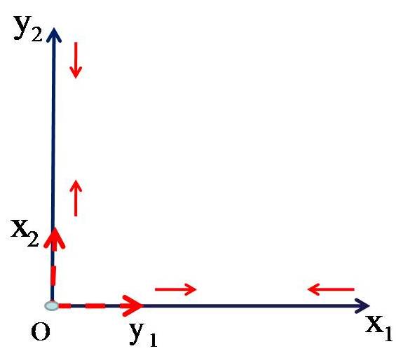
Figure 3: Illustration of the first example. $X=(x_{1}^{T},x_{2}^{T})=\mathrm{Diag}\left(x_{11},x_{22}\right)$, $Y=(y_{1}^{T},y_{2}^{T})=\mathrm{Diag}\left(y_{11},y_{22}\right)$, where $x_{11}=y_{22}\gg x_{22}=y_{11}$ and $x_{11}y_{11}=x_{22}y_{22}=1-d/\sqrt{2}$. We use the following operation to define $U,V$: shrink $x_{1}$ and extend $x_{2}$ to obtain $U$, while keeping the norm invariant (i.e. $\|U\|_{F}=\|X\|_{F}$); shrink $y_{2}$ and extend $y_{1}$ to obtain $V$, while keeping the norm invariant (i.e. $\|V\|_{F}=\|Y\|_{F}$). We can prove that there exists an operation such that $u_{ii}v_{ii}=1>x_{ii}y_{ii},i=1,2$.

How should we define $U=\mathrm{Diag}(u_{11},u_{22}),V=\mathrm{Diag}(v_{11},v_{22})$ so that (114) holds? Due to the “symmetry” of $X$ and $Y$ in this example (by symmetry we mean $x_{11}=y_{22},x_{22}=y_{11}$), we choose $U,V$ such that $u_{11}=v_{22},u_{22}=v_{11}$. Then the requirements (114a) and (114b) reduce to:

$$\begin{split}u_{11}u_{22}=1=\frac{x_{11}x_{22}}{1-d/\sqrt{2}},\\ u_{11}^{2}+u_{22}^{2}\leq x_{11}^{2}+x_{22}^{2}.\end{split}$$ (117)

It can be easily shown that there exist $u_{11},u_{22}$ satisfying (117). In fact, define $R=\|X\|_{F}=\sqrt{x_{11}^{2}+x_{22}^{2}}$ and let a point $(w_{1},w_{2})$ move along the circle $\{(w_{1},w_{2})\mid w_{1}^{2}+w_{2}^{2}=R^{2}\}$ from $(x_{11},x_{22})$ to $(R/\sqrt{2},R/\sqrt{2})$. During this process, the norm of $(w_{1},w_{2})$ does not change and the product $w_{1}w_{2}$ monotonically increases from $x_{11}x_{22}$ to $R^{2}/2$. Therefore, there exist $u_{11},u_{22}$ satisfying (117) as long as $R^{2}/2>x_{11}x_{22}/(1-d/\sqrt{2})$. This inequality is equivalent to $(1-d/\sqrt{2})(x_{11}^{2}+x_{22}^{2})/2>x_{11}x_{22}$, which can be simplified to $(1-d/\sqrt{2})(x_{11}-x_{22})^{2}>\sqrt{2}dx_{11}x_{22}=\sqrt{2}d(1-d/\sqrt{2})$, or equivalently, $(x_{11}-x_{22})^{2}>\sqrt{2}d$. The last inequality holds when $x_{11}-x_{22}=C-(1-d/\sqrt{2})/C$ is large enough (i.e. $C$ is large enough).

To summarize, we will increase the small entry $x_{22}$ (resp.$\ y_{11}$) and decrease the large entry $x_{11}$ (resp.$\ y_{22}$) to obtain a more balanced diagonal matrix $U$ (resp.$\ V$), which has the same norm as $X$ (resp.$\ Y$). The percentage of increase in the small entry $x_{22}$ (resp.$\ y_{11}$) will be much larger than the percentage of decrease in the large entry $x_{11}$ (resp.$\ y_{22}$), thus the products $x_{22}y_{22}$ and $x_{11}y_{11}$ will increase; in other words, the product $UV^{T}$ of the more balanced matrices $U,V$ will have larger entries than $XY^{T}$.

Note that the above idea of shrinking/extending works when there is a large imbalance in the lengths of the rows of $X,Y$, regardless of whether $X,Y$ are diagonal matrices or not. By the assumption that $\|X\|_{F}$ and $\|Y\|_{F}$ are large, we know that there must be a row of $X$ (resp.$\ Y$) that has large norm (here “large” means much larger than $1/\sqrt{r}$); however, it is possible that all rows of $X$ and $Y$ have large norm and there is no imbalance in terms of the lengths of the rows. See below for such an example.

In the second example (see Figure 4), we still set $r=2$, $\Sigma=I$, $d=1/(C_{d}r)$. Suppose $X=(x_{1}^{T},x_{2}^{T})$, $Y=(y_{1}^{T},y_{2}^{T})$. We define $x_{1}=(C,0),x_{2}=(-C\sin\alpha,C\cos\alpha)$ and $y_{1}=(C\cos\alpha,C\sin\alpha),y_{2}=(0,C)$, where $C$ is a large constant, and $\alpha\in(0,\pi/2)$ is chosen so that

$$C^{2}\cos\alpha=1-d/\sqrt{2}.$$ (118)

When $C$ is large, $\alpha\approx\arccos(1/C^{2})$ is also large (i.e. close to $\pi/2$). Condition (112) holds since $\|XY^{T}-\Sigma\|_{F}=\|C^{2}\cos\alpha I-I\|_{F}=\|(1-d/\sqrt{2})I-I\|_{F}=d=1/(C_{d}r)$. Note that $\|X\|_{F}=\|Y\|_{F}=\sqrt{2}C$, so we can choose $C=\beta_{T}/\sqrt{2}=\sqrt{2C_{T}}/\sqrt{2}=\sqrt{C_{T}}$ so that (113) holds.

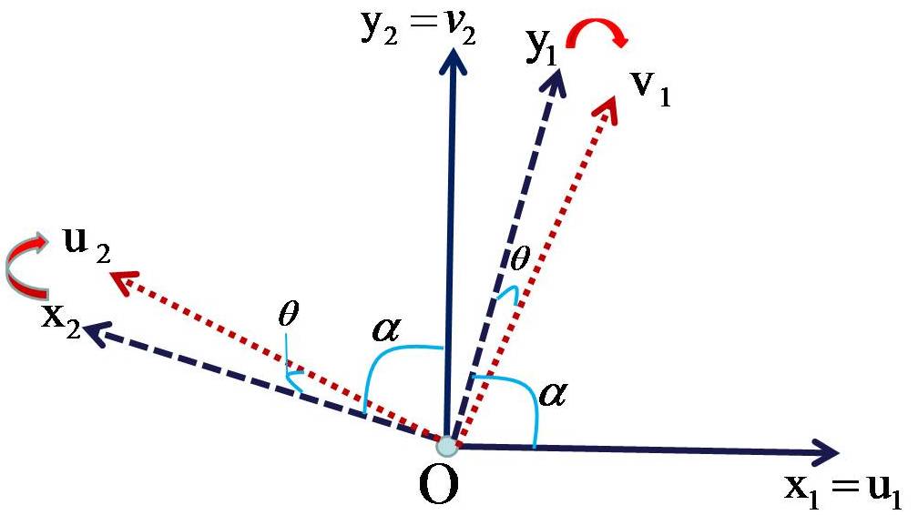
Figure 4: Illustration of the second example. $X=(x_{1}^{T},x_{2}^{T})$, $Y=(y_{1}^{T},y_{2}^{T})$, where $x_{1}=(C,0),x_{2}=(-C\sin\alpha,C\cos\alpha)$ and $y_{1}=(C\cos\alpha,C\sin\alpha),y_{2}=(0,C)$, where $C$ is a large constant. Choose $\alpha$ so that $C^{2}\cos\alpha=1-d/\sqrt{2}$. We use the following operation to define $U=(u_{1}^{T},u_{2}^{T})$, $V=(v_{1}^{T},v_{2}^{T})$: rotate $y_{1}$ (resp.$\ x_{2}$) by angle $\theta$ to obtain $v_{1}$(resp.$\ u_{2}$), and let $u_{2}=x_{2},v_{1}=y_{1}$. Here the angle of rotation $\theta$ is chosen so that $\langle u_{1},v_{1}\rangle=\langle u_{2},v_{2}\rangle=1$.

How should we choose $U=(u_{1}^{T},u_{2}^{T})$, $V=(v_{1}^{T},v_{2}^{T})$ so that (114) holds? The idea for the first example no longer works since it requires that the difference of $\|x_{1}\|$ and $\|x_{2}\|$ (resp.$\ \|y_{1}\|$ and $\|y_{2}\|$) is large; however, in this example, $\|x_{1}\|-\|x_{2}\|=\|y_{1}\|-\|y_{2}\|=0$. The key idea for this example is to use rotation. Rotating a vector does not change the norm, so requirement (113) will not be violated if $u_{i}$ (resp.$\ v_{i}$) is obtained by rotating $x_{i}$(resp.$\ y_{i}$). For simplicity, we rotate $y_{1},x_{2}$ to obtain $v_{1},u_{2}$ respectively and let $u_{1}=x_{1},v_{2}=y_{2}$ (see Figure 4). Note that $y_{1}$ and $x_{2}$ should be rotated by the same angle as $v_{1}$ should be orthogonal to $u_{2}$ (since the off-diagonal entries of $UV^{T}$ are zero). To increase the inner product $\langle x_{i},y_{i}\rangle$ from $1-d/\sqrt{2}$ to $1$, we need to decrease the angle of $x_{i}$ and $y_{i}$, thus $y_{1}$ (resp.$\ x_{2}$) should be rotated towards $x_{1}$(resp.$\ y_{2}$). Finally, let us specify the angle of rotation $\theta\triangleq\angle(y_{1},v_{1})=\angle(x_{2},u_{2})$. The requirement $\langle u_{1},v_{1}\rangle=1$ is equivalent to $1=\|u_{1}\|\|v_{1}\|\cos\angle(u_{1},v_{1})=\|x_{1}\|\|y_{1}\|\cos(\alpha-\theta),$ which can be rewritten as

$$1=C^{2}\cos(\alpha-\theta).$$ (119)

The right-hand side of (119) is an increasing function of $\theta$, ranging from $C^{2}\cos(\alpha)\overset{\eqref{C square cos alpha}}{=}1-d/\sqrt{2}$ to $C^{2}$ for $\theta\in[0,\alpha]$. Since $1$ lies in the range $[1-d/\sqrt{2},C^{2}]$, there exists a unique $\theta$ so that (119) holds. One can further verify the requirement (114c), i.e. the difference of $X$ (resp.$\ Y$) and $U$ (resp.$\ V$) is small. As a rough summary, we rotate $x_{i},y_{i}$ to obtain $u_{i},v_{i}$ when the angle of $x_{i}$ and $y_{i}$ is large. This operation does not change the norm and can increase the inner product $\langle x_{i},y_{i}\rangle$ to the desired amount ($1$ in this case).

C.2.3 Proof Ideas of Proposition C.1

In the above two examples, we have used two different operations: one is based on shrinking/extending, and the other is based on rotation. As we mentioned before, the first operation cannot deal with the second example; also, it is obvious that the second operation cannot deal with the first example (the angle between $x_{i}$ and $y_{i}$ is zero, so rotation only decreases the inner product). Therefore, both operations are necessary.

Are these two operations sufficient? Fortunately, the answer is yes for the case that $XY^{T}$ is diagonal and $\langle x_{i},y_{i}\rangle\leq\Sigma_{i}$ (we need extra effort to reduce the general problem to this case). When all the angles between $x_{i}$ and $y_{i}$ are smaller than a constant $\bar{\alpha}$, there must be some kind of imbalance in the lengths of $x_{i},y_{i}$’s (to illustrate this, if all $\|x_{i}\|=\|y_{i}\|$, then $\|x_{i}\|^{2}=\|x_{i}\|\|y_{i}\|\approx\Sigma_{i}/\cos\angle(x_{i},y_{i})\leq\Sigma_{i}/\cos(\bar{\alpha})$, which implies $\|X\|_{F}^{2}\lesssim r\Sigma_{\rm max}/\cos(\bar{\alpha})\ll\frac{3}{5}C_{T}r\Sigma_{\rm max}=\frac{3}{5}\beta_{T}^{2}$ for large enough $C_{T}$, a contradiction to (112)). Thus we can use the first operation (i.e. shrinking/extending the vectors $x_{i},y_{i}$’s) to obtain the desired $U,V$. When all the angles between $x_{i}$ and $y_{i}$ are larger than a constant $\bar{\alpha}$, we can use the second operation (i.e. rotating the vectors $x_{i},y_{i}$’s) to obtain the desired $U,V$. In general, some angles may be larger than $\bar{\alpha}$ and others may be smaller, then a natural solution is to use the two operations simultaneously: use the first operation for the pairs $(x_{i},y_{i})$ with small angles and the second operation for those with large angles.

We had a proof using the two operations simultaneously, but the bounds on $\|U-X\|_{F},\|V-Y\|_{F}$ have a large exponent of $r$. In the following subsection, we present a different proof that does not use the two operations simultaneously, but only use one of the two operations. The basic proof framework is summarized as follows. We first define $\hat{Y}$ so that $X\hat{Y}=\Sigma$; in other words, we try to satisfy the requirement (114a) first. Then we try to modify $\hat{Y}$ to satisfy the requirement (114b). In particular, we need to reduce the norm of $\hat{Y}$ and keep the norm of $X$ unchanged, while maintaining the relation $X\hat{Y}^{T}=\Sigma$. We consider two cases: in Case 1, “most” angles between $X$ and $\hat{Y}$ are smaller than $\bar{\alpha}$, and using the first operation (shrinking/extending) can obtain the desired $U,V$; in Case 2, “most” angles between $X$ and $\hat{Y}$ are larger than $\bar{\alpha}$, and using the second operation (rotation) can obtain the desired $U,V$ (see (127) for a precise definition of Case 1 and Case 2). The difference of this proof framework and the previous one is the following. In our previous proof framework, we need to take into account every pair $x_{i},y_{i}$ so that its inner product is modified to $\Sigma_{i}$, thus two operations have to be applied simultaneously. In contrast, in this new proof framework, $\langle x_{i},\hat{y}_{i}\rangle$ is already $\Sigma_{i}$, and we only need to worry about the “overall” requirement that $\|\hat{Y}\|_{F}$ should be reduced, thus dealing only with the pairs with small angles (or only with the pairs with large angles) is enough to satisfy the requirement.

Finally, we would like to mention that when $\Sigma$ is an identity matrix, the proof can be rather simple. In fact, in this case one can assume $X$ to be diagonal by proper orthonormal transformation, and then assume $Y$ to be diagonal since the off-diagonal entries are small. By just using the first operation (scaling of the diagonal entries), we can construct the desired $U,V$ and the proof is similar to that in Appendix C.3.1. When $\Sigma$ is not a diagonal matrix, we can replace $X,Y$ by $XQ,Q^{-1}Y$ where $Q$ is orthonormal, but that only simplifies $X$ to a upper triangular matrix, a condition seems not very helpful. It seems that the second operation has to be used and the proof becomes more involved.

C.3 Proof of Proposition C.1

As mentioned earlier, to simplify the notations, we use $X,Y,U,V,d$ to replace $X_{1}^{\prime},Y_{1}^{\prime},U_{1}^{\prime},V_{1}^{\prime},d^{\prime}$ in Proposition (C.1). Throughout the proof, we choose

$$C_{T}=20,$$ (120)

and $C_{d}=108$, which implies

$$\frac{d}{\Sigma_{\rm min}}\leq\frac{1}{108r}.$$ (121)

There are two “hard” requirements on $U,V$: (114a) and (114b). Our construction of $U,V$ can be viewed as a two-step approach, whereby we satisfy one requirement in each step. In Step 1, we construct

$$\hat{Y}=\Sigma(\Sigma+D)^{-T}Y,\quad\text{where }D\triangleq XY^{T}-\Sigma,$$

then

$$X\hat{Y}^{T}=(XY^{T})(XY^{T})^{-1}\Sigma=\Sigma,$$

i.e. the first requirement is satisfied. Since the new $\hat{Y}$ may have higher norm than $\|Y\|_{F}$, in Step 2 we modify $X,\hat{Y}$ to $U,V$ so that the product does not change, and $\|V\|_{F}\leq\|Y\|_{F},\|U\|_{F}\leq\|X\|_{F}$.

Claim C.1

Let $\hat{Y}=\Sigma(\Sigma+D)^{-T}Y$, then

$$\eta\triangleq 1-\frac{\|Y\|_{F}}{\|\hat{Y}\|_{F}}\leq\frac{d}{\Sigma_{\rm min}},$$ (122a)

$$\|Y-\hat{Y}\|_{F}\leq\frac{d}{\Sigma_{\rm min}-d}\|Y\|_{F}.$$ (122b)

Proof of Claim C.1: By the definition of $\hat{Y}$ we have $Y=(\Sigma+D)^{T}\Sigma^{-1}\hat{Y}$, then we have

$$\begin{split}\|Y-\hat{Y}\|_{F}=\|(\Sigma+D)^{T}\Sigma^{-1}\hat{Y}-\hat{Y}\|_{F}=\|D^{T}\Sigma^{-1}\hat{Y}\|_{F}\\ \leq\|D^{T}\Sigma^{-1}\|_{F}\|\hat{Y}\|_{F}\leq\|D^{T}\|_{F}\Sigma_{\rm min}^{-1}\|\hat{Y}\|_{F}=\frac{d}{\Sigma_{\rm min}}\|\hat{Y}\|_{F}.\end{split}$$ (123)

Using the triangular inequality and (123), we have

$$\|\hat{Y}\|_{F}\leq\|Y-\hat{Y}\|_{F}+\|Y\|_{F}\leq\frac{d}{\Sigma_{\rm min}}\|\hat{Y}\|_{F}+\|Y\|_{F},$$

$$\Longrightarrow\quad \|Y\|_{F}\geq(1-\frac{d}{\Sigma_{\rm min}})\|\hat{Y}\|_{F}.$$ (124)

The first desired inequality (122a) follows immediately from (124), and the second desired inequality (122b) is proved by combining (124) and (123). $\Box$

Combining (122a) and (121), we obtain

$$\eta\leq\frac{1}{108r}.$$ (125)

If $\eta\leq 0$, i.e. $\|\hat{Y}\|_{F}\leq\|Y\|_{F}$, then $U=X,V=\hat{Y}$ already satisfy (114). From now on, we assume $\eta>0,$ i.e. $\|\hat{Y}\|_{F}>\|Y\|_{F}$. Denote $x_{i}^{T},\hat{y}_{i}^{T},u_{i}^{T},v_{i}^{T}$ as the $i$-$th$ row of $X,\hat{Y},U,V$, respectively. Denote $\alpha_{i}\triangleq\angle(x_{i},\hat{y}_{i})$, i.e. the angle between the two vectors $x_{i}$ and $\hat{y}_{i}$. Since $\langle x_{i},\hat{y}_{i}\rangle=\Sigma_{i}>0$, we have $\alpha_{i}\in[0,\frac{\pi}{2})$. Without loss of generality, assume

$$\alpha_{1},\dots,\alpha_{s}>\frac{3}{8}\pi,\quad\alpha_{s+1},\dots,\alpha_{r}\leq\frac{3}{8}\pi,$$ (126)

where $s\in\{0,1,\dots,r\}$. We consider three cases and construct $U,V$ that satisfy the desired properties in the subsequent three subsections.

$$\text{Case 1}: \quad\sum_{i=s+1}^{r}\|\hat{y}_{i}\|^{2}\geq\frac{2}{3}\|\hat{Y}\|_{F}^{2},\;\;\sum_{i=s+1}^{r}\|x_{i}\|^{2}\geq\frac{2}{3}\|X\|_{F}^{2}.$$ (127a)

$$\text{Case 2a}: \quad\sum_{i=1}^{s}\|\hat{y}_{i}\|^{2}>\frac{1}{3}\|\hat{Y}\|_{F}^{2}.$$ (127b)

$$\text{Case 2b}: \quad\sum_{i=1}^{s}\|x_{i}\|^{2}>\frac{1}{3}\|X\|_{F}^{2}.$$ (127c)

C.3.1 Proof of Case 1

Without loss of generality, assume

$$\|x_{s+1}\|\leq\|x_{s+2}\|\leq\dots\leq\|x_{r}\|.$$ (128)

Let $K$ be the smallest integer in $\{s+1,s+2,\dots,r\}$ so that

$$\sum_{i=s+1}^{K}\|\hat{y}_{i}\|^{2}\geq 2\sum_{j=K+1}^{r}\|\hat{y}_{j}\|^{2}.$$ (129)

By this definition of $K$, we have

$$\sum_{i=s+1}^{K-1}\|\hat{y}_{i}\|^{2}<2\sum_{j=K}^{r}\|\hat{y}_{j}\|^{2}.$$ (130)

We will shrink and extend $x_{i},\hat{y}_{i}$ to obtain $U,V$. The precise definition of $U=(u_{1},u_{2},\dots,u_{r})^{T},V=(v_{1},\dots,v_{r})^{T}$ is given in Table 8.

Table 8: Operation 1

Operation 1: Shrinking and Extending
Input: $x_{k},\hat{y}_{k},k=1,\dots,r$.
Output: $u_{k},v_{k},k=1,\dots,r$.
Procedure:
(i) For each $j\leq s$, keep $x_{j},\hat{y}_{j}$ unchanged, i.e.  $$u_{j}\triangleq x_{j},\;v_{j}\triangleq\hat{y}_{j},\;\;j=1,\dots,s.\vspace{-0.6cm}$$ (131)
(ii) For each $i\in\{s+1,\dots,K\}$, extend $x_{i}$ to obtain $u_{i}$ and shrink $\hat{y}_{i}$ to obtain $v_{i}$. For each $i\geq K+1$, shrink $x_{i}$ to obtain $u_{i}$ and extend $\hat{y}_{i}$ to obtain $v_{i}$. More specifically, $$u_{i}\triangleq\frac{x_{i}}{1-\epsilon_{i}},v_{i}\triangleq\hat{y}_{i}(1-\epsilon_{i}),\text{ where }\epsilon_{i}=\begin{cases}7\bar{\eta}&i\leq K,\\ -4.5\bar{\eta}&i\geq K+1,\end{cases}\quad i=s+1,s+2,\dots,r,\vspace{-0.4cm}$$ (132) in which $$\bar{\eta}\triangleq\frac{d}{\Sigma_{\min}}\geq\eta.$$ (133)

We will show that such $U,V$ satisfy the requirements (114). The requirement (114a) follows directly from the definition of $U,V$ and the fact $X\hat{Y}^{T}=\Sigma$.

We then prove the requirement (114c). We can bound $\|U-X\|_{F}$ as

$$\begin{split}\|U-X\|_{F}=\sqrt{\sum_{i>s}\|\frac{1}{1-\epsilon_{i}}x_{i}-x_{i}\|^{2}}=\sqrt{\sum_{i>s}\left(\frac{\epsilon_{i}}{1-\epsilon_{i}}\right)^{2}\|x_{i}\|^{2}}\\ \leq\frac{7\bar{\eta}}{1-7\bar{\eta}}\sqrt{\sum_{i>s}\|x_{i}\|^{2}}\leq\frac{7\bar{\eta}}{1-7\bar{\eta}}\|X\|_{F}\leq\frac{15}{2}\bar{\eta}\beta_{T}.\end{split}$$ (134)

The bound of $\|V-\hat{Y}\|_{F}$ is given as

$$\|V-\hat{Y}\|_{F}=\sqrt{\sum_{i>s}\|(1-\epsilon_{i})\hat{y}_{i}-\hat{y}_{i}\|^{2}}\leq\sqrt{\sum_{i>s}\epsilon_{i}^{2}\|\hat{y}_{i}\|^{2}}\leq 7\bar{\eta}\|\hat{Y}\|_{F}.$$

Combining with the bound (123), we can bound $\|V-Y\|_{F}$ as

$$\begin{split}\|V-Y\|_{F}\leq\|V-\hat{Y}\|_{F}+\|\hat{Y}-Y\|_{F}\leq 7\bar{\eta}\|\hat{Y}\|_{F}+\frac{d}{\Sigma_{\rm min}}\|\hat{Y}\|_{F}\\ =8\bar{\eta}\|\hat{Y}\|_{F}\overset{\eqref{eta bound}}{\leq}\frac{8\bar{\eta}}{1-\bar{\eta}}\|Y\|_{F}\leq\frac{58}{7}\bar{\eta}\beta_{T}.\end{split}$$ (135)

The first part of the requirement (114c) now follows by multiplying (134) and (135), and the second part of the requirement (114c) follows directly from (134) and (135).

At last, we prove that $U,V$ satisfy the requirement (114b). Let

$$S_{1}\triangleq\sum_{i=s+1}^{K}\|\hat{y}_{i}\|^{2},\;S_{2}\triangleq\sum_{j=K+1}^{r}\|\hat{y}_{j}\|^{2},\;S_{3}\triangleq\sum_{k=1}^{s}\|\hat{y}_{k}\|^{2},$$

then (129) and (127a) imply

$$S_{2}\leq S_{1}/2,\;\;S_{3}\leq(S_{1}+S_{2})/2\leq 3S_{1}/4.$$ (136)

Since $\bar{\eta}=d/\Sigma_{\min}\geq\eta$, we have $(1-\eta)^{2}(1-\bar{\eta})^{2}\geq(1-2\eta)(1-2\bar{\eta})\geq(1-2\bar{\eta})^{2}$. Then

$$\begin{split}&(1-\eta)^{2}(1-\bar{\eta})^{2}\|\hat{Y}\|_{F}^{2}-\|V\|_{F}^{2}\\ &\geq(1-2\bar{\eta})^{2}\|\hat{Y}\|_{F}^{2}-\|V\|_{F}^{2}\\ &=\sum_{i\geq s+1}((1-2\bar{\eta})^{2}\|\hat{y}_{i}\|^{2}-\|v_{i}\|^{2})+\sum_{k\leq s}((1-2\bar{\eta})^{2}\|\hat{y}_{k}\|^{2}-\|v_{k}\|^{2})\\ &=\sum_{i\geq s+1}((1-2\bar{\eta})^{2}\|\hat{y}_{i}\|^{2}-(1-\epsilon_{i})^{2}\|\hat{y}_{i}\|^{2})\\ &\quad\quad+\sum_{k\leq s}((1-2\bar{\eta})^{2}\|\hat{y}_{k}\|^{2}-\|\hat{y}_{k}\|^{2})\\ &=\sum_{i\geq s+1}(\epsilon_{i}-2\bar{\eta})(2-\epsilon_{i}-2\bar{\eta})\|\hat{y}_{i}\|^{2}-\sum_{k\leq s}4\bar{\eta}(1-\bar{\eta})\|\hat{y}_{k}\|^{2}\\ &\overset{\eqref{eps and u,v def}}{=}\sum_{s+1\leq i\leq K}5\bar{\eta}(2-5\bar{\eta}-2\bar{\eta})\|\hat{y}_{i}\|^{2}\\ &\quad\quad+\sum_{K<j\leq r}(-6.5\bar{\eta})(2+4.5\bar{\eta}-\bar{\eta})\|\hat{y}_{j}\|^{2}-\sum_{k\leq s}4\bar{\eta}(1-\bar{\eta})\|\hat{y}_{k}\|^{2}\\ &=5\bar{\eta}(2-7\bar{\eta})S_{1}-6.5\bar{\eta}(2+2.5\bar{\eta})S_{2}-4\bar{\eta}(1-\bar{\eta})S_{3}\\ &\overset{\eqref{S_1, S_2 bound}}{\geq}5\bar{\eta}(2-7\bar{\eta})S_{1}-6.5\bar{\eta}(2+2.5\bar{\eta})\frac{1}{2}S_{1}-4\bar{\eta}(1-\bar{\eta})\frac{3}{4}S_{1}\\ &\geq(0.5-41\bar{\eta})\bar{\eta}S_{1}\geq 0,\end{split}$$ (137)

where the last inequliaty follows from (121). Note that $(1-\eta)\|\hat{Y}\|_{F}=\|Y\|_{F}$, thus (137) implies

$$\|V\|_{F}\leq(1-\eta)(1-\bar{\eta})\|\hat{Y}\|_{F}=(1-\frac{d}{\Sigma_{\min}})\|Y\|_{F},$$

which proves the second part of (114b).

We then prove the first part of (114b), i.e. $\|U\|_{F}\leq\|X\|_{F}$. Let

$$T_{1}\triangleq\sum_{i=s+1}^{K}\|x_{i}\|^{2},\;\;T_{2}\triangleq\sum_{j=K}^{r}\|x_{j}\|^{2}.$$

We claim that

$$T_{2}\geq 2T_{1}.$$ (138)

We prove (138) by contradiction. Assume the contrary that $T_{2}<2T_{1}$, then $\frac{1}{3}(T_{2}+T_{1})<T_{1}$, i.e.

$$\frac{1}{3}\sum_{k=s+1}^{r}\|x_{k}\|^{2}<\sum_{i=s+1}^{K}\|x_{i}\|^{2}\overset{\eqref{order x_i norm}}{\leq}(K-s)\|x_{K}\|^{2}.$$ (139)

Plugging the second inequality of (127a), i.e.  $\sum_{k=s+1}^{r}\|x_{k}\|^{2}\geq\frac{2}{3}\|X\|_{F}^{2}$, into the above relation, we obtain

$$\|X\|_{F}^{2}\leq\frac{9}{2}(K-s)\|x_{K}\|^{2}\leq\frac{9}{2}K\|x_{K}\|^{2}.$$ (140)

When $j\in\{K,K+1,\dots,r\}$, we have

$$\Sigma_{\rm max}\geq\Sigma_{j}=\langle x_{j},\hat{y}_{j}\rangle=\|x_{j}\|\|\hat{y}_{j}\|\cos(\alpha_{j})\overset{\eqref{order x_i norm},\eqref{angle threshold, for s}}{\geq}\|x_{K}\|\|\hat{y}_{j}\|\cos(3\pi/8).$$

which implies

$$\|\hat{y}_{j}\|\leq\omega,\text{ where }\omega\triangleq\frac{1}{\cos(3\pi/8)}\frac{\Sigma_{\rm max}}{\|x_{K}\|},\;\;j=K,K+1,\dots,s.$$ (141)

Therefore,

$$\|\hat{Y}\|_{F}^{2}\overset{\eqref{category 1}}{\leq}\frac{3}{2}\sum_{j=s+1}^{r}\|\hat{y}_{j}\|^{2}\overset{\eqref{K-1 does not satisfy S1 > 2S2}}{\leq}\frac{9}{2}\sum_{j=K}^{r}\|\hat{y}_{j}\|^{2}\overset{\eqref{omega bound hat yj}}{\leq}\frac{9}{2}(r-K+1)\omega^{2}.$$ (142)

Combining (140) and (142), and using $K(r-K+1)\leq\frac{1}{4}(r+1)^{2}\leq r^{2}$, we get

$$\begin{split}\|X\|_{F}^{2}\|\hat{Y}\|_{F}^{2}\leq\frac{81}{4}r^{2}\|x_{K}\|^{2}\omega^{2}\\ \overset{\eqref{omega bound hat yj}}{=}\frac{81}{4}r^{2}\|x_{K}\|^{2}\frac{1}{\cos(3\pi/8)^{2}}\frac{\Sigma_{\rm max}^{2}}{\|x_{K}\|^{2}}<140r^{2}\Sigma_{\rm max}^{2}.\end{split}$$ (143)

According to (113), we have $\|X\|_{F}^{2}\|\hat{Y}\|_{F}^{2}\geq\|X\|_{F}^{2}\|Y\|_{F}^{2}\geq(\frac{3}{5})^{2}\beta_{T}^{4}=\frac{9}{25}C_{T}^{2}r^{2}\Sigma_{\rm max}^{2}$; combining with (143), we get $140>\frac{9}{25}C_{T}^{2}$, which implies $C_{T}^{2}<389$. This contradicts the definition (120) that $C_{T}=20$, thus (138) is proved.

Now we are ready to prove the first part of (114b) as follows:

$$\begin{split}\|X\|_{F}^{2}-\|U\|_{F}^{2}&=\sum_{i\geq s+1}(\|x_{i}\|^{2}-\|u_{i}\|^{2})+\sum_{k\leq s}(\|x_{k}\|^{2}-\|u_{k}\|^{2})\\ &=\sum_{i\geq s+1}(\|x_{i}\|^{2}-\frac{1}{(1-\epsilon_{i})^{2}}\|x_{i}\|^{2})+0\\ &=\sum_{i\geq s+1}\frac{\epsilon_{i}(\epsilon_{i}-2)}{(1-\epsilon_{i})^{2}}\|x_{i}\|^{2}\\ &=\sum_{K<j\leq r}\frac{4.5\bar{\eta}(4.5\bar{\eta}+2)}{(1+4.5\bar{\eta})^{2}}\|x_{j}\|^{2}-\sum_{s+1\leq i\leq K}\frac{7\bar{\eta}(2-7\bar{\eta})}{(1-7\bar{\eta})^{2}}\|x_{i}\|^{2}\\ &\overset{\eqref{T1 > 0.3 T2}}{\geq}T_{2}\bar{\eta}\left[\frac{4.5(4.5\bar{\eta}+2)}{(1+4.5\bar{\eta})^{2}}-\frac{1}{2}\frac{7(2-7\bar{\eta})}{(1-7\bar{\eta})^{2}}\right]\\ &\geq T_{2}\bar{\eta}\left[\frac{9}{(1+4.5\bar{\eta})^{2}}-\frac{7}{(1-7\bar{\eta})^{2}}\right]\geq 0,\end{split}$$

where the last inequality is because $\frac{(1-7\bar{\eta})^{2}}{(1+4.5\bar{\eta})^{2}}>0.79>\frac{7}{9}$ when $\bar{\eta}\leq 1/(108r)<1/100$. Thus the first part of (114b) is proved.

C.3.2 Proof of Case 2a

Denote

$$X^{0}=X,Y^{0}=\hat{Y},x_{k}^{0}=x_{k},y_{k}^{0}=\hat{y}_{k},\alpha_{k}^{0}=\alpha_{k},\;k=1,\dots,r.$$ (144)

We will define $X^{i}=(x_{1}^{i},\dots,x_{r}^{i})^{T},Y^{i}=(y_{1}^{i},\dots,y_{r}^{i})^{T}$ recursively. In specific, at the $i$-th iteration, we will adjust $X^{i-1},Y^{i-1}$ to $X^{i},Y^{i}$ so that $\|X^{i}\|_{F}\leq\|X^{i-1}\|_{F},\|Y^{i}\|_{F}<\|Y^{i-1}\|_{F}$ while keeping the first requirement satisfied, i.e. $X^{i}(Y^{i})^{T}=\Sigma$. The angle $\alpha_{k}^{i}$ is defined accordingly, i.e. $\alpha_{k}^{i}\triangleq\langle x_{k}^{i},y_{k}^{i}\rangle$.

To adjust $X^{i-1},Y^{i-1}$ to $X^{i},Y^{i}$, we will define an operation that consists of rotation and shrinking. The basic idea is the following: since the angle between $x_{i}^{i-1}$ and $y_{i}^{i-1}$ is large, we can rotate $x_{i}^{i-1}$ to $x_{i}^{i}$ and shrink $y_{i}^{i-1}$ to $y_{i}^{i}$ to keep the inner product invariant, i.e. $\langle x_{i}^{i-1},y_{i}^{i-1}\rangle=\langle x_{i}^{i},y_{i}^{i}\rangle$. However, rotating $x_{i}^{i-1}$ may destroy the orthogonal relationship between $x_{i}^{i-1}$ and $y_{j}^{i-1},\forall j\neq i$, thus we further rotate and shrink $y_{j}^{i-1}$ to $y_{j}^{i}$ for all $j\neq i$ so that $y_{j}^{i}$ is orthogonal to the new vector $x_{i}^{i}$. Fortunately, we can prove that using such an operation we still have $\langle x_{j}^{i-1},y_{j}^{i}\rangle=\Sigma_{j},\forall j\neq i$.

A complete description of this operation is given in Table 9. Without loss of generality, we can make the assumption (145). In fact, if (145) does not hold, we can switch $i$ and $m_{i}\triangleq\arg\min_{k\in\{i,i+1,\dots,s\}}\alpha_{k}^{i-1}$ and then apply Operation 2.

Table 9: Operation 2 that defines $X^{i},Y^{i}$, where $i\in\{1,\dots,s\}$

Operation 2: Rotation and Shrinking
Input: $x_{k}^{i-1},y_{k}^{i-1},\alpha_{k}^{i-1}\triangleq\angle(x_{k}^{i-1},y_{k}^{i-1}),k=1,\dots,r$ and $D_{i}$.
Output: $x_{k}^{i},y_{k}^{i},k=1,\dots,r$ and $\alpha_{k}^{i}\triangleq\angle(x_{k}^{i},y_{k}^{i})$.
Procedure:
(1) Rotate $x_{i}^{i-1}$ in $\mathrm{span}\{x_{i}^{i-1},y_{i}^{i-1}\}$ to get $x_{i}^{i}$, such that $\langle x_{i}^{i},y_{i}^{i-1}\rangle=\Sigma_{i}+D_{i}.$
(2) Shrink $y_{i}^{i-1}$ to get $y_{i}^{i}$ such that $\langle x_{i}^{i},y_{i}^{i}\rangle=\Sigma_{i}.$
(3) For all $j\neq i$, find $y_{j}^{i}$ in $\mathrm{span}\{y_{j}^{i-1},y_{i}^{i-1}\}=\mathrm{span}_{k\neq i,j}\{x_{k}^{i-1}\}^{\bot}$ such that $y_{j}^{i}\bot x_{i}^{i}$ and $\langle x_{j}^{i-1},y_{j}^{i}\rangle=\langle x_{j}^{i-1},y_{j}^{i-1}\rangle.$
(4) Define $x_{j}^{i}\triangleq x_{j}^{i-1},\forall j\neq i$.

We will prove that Operation 2 is valid (for $D_{i}$ that is small enough), i.e. $X^{i},Y^{i}$ defined in Operation 2 indeed exist. The properties of $X^{i},Y^{i}$ obtained by Operation 2 are summarized in the following claim, which will be proved in Appendix C.4.

Claim C.2

Consider $i\in\{1,2,\dots,s\}$. Suppose

$$\alpha_{i}^{i-1}\leq\alpha_{j}^{i-1},\;\forall\ j\in\{i+1,i+2,\dots,s\},$$ (145)

and $D_{i}>0$ satisfies

$$\frac{D_{i}}{\Sigma_{i}}\leq\frac{1}{12r},$$ (146)

then $X^{i}=(x_{1}^{i},\dots,x_{r}^{i})^{T},Y^{i}=(y_{1}^{i},\dots,y_{r}^{i})^{T}$ described in Operation 2 exist and satisfy the following properties:

$$X^{i}(Y^{i})^{T} =\Sigma,$$ (147a)

$$\quad\|x_{k}^{i}\|=\|x_{k}^{i-1}\|,\forall k,\;\;\|Y^{i}-Y^{i-1}\|_{F}^{2} \leq\frac{4}{5}\frac{D_{i}}{\Sigma_{i}}(\|Y^{i-1}\|_{F}^{2}-\|Y^{i}\|_{F}^{2}),$$ (147b)

$$\|X^{i}-X^{i-1}\|_{F}=\|x_{i}^{i}-x_{i}^{i-1}\|\leq \frac{1}{\sqrt{3}}\frac{D_{i}}{\Sigma_{i}}\|x_{i}^{i-1}\|$$

$$\;\;\|Y^{i}-Y^{i-1}\|_{F} \leq\frac{2}{\sqrt{3}}\frac{D_{i}}{\Sigma_{i}}\|Y^{i-1}\|_{F},$$ (147c)

$$\alpha_{l}^{i}\geq\alpha_{l}^{i-1}-\frac{1}{r}\frac{\pi}{24}\geq\frac{1}{3}\pi, \;l=i,i+1,\dots,s.$$ (147d)

$$\|y_{k}^{i-1}\|\geq\|y_{k}^{i}\|\geq\|y_{k}^{i-1}\|-\frac{1}{10r}\| y_{k}^{i-1}\|,\;k=1,2,\dots,s.$$ (147e)

$$\|Y^{i-1}\|_{F}^{2}-\|Y^{i}\|_{F}^{2}\geq \frac{5}{3}\frac{D_{i}}{\Sigma_{i}}\|y_{i}^{i}\|^{2}.$$ (147f)

We continue to prove Proposition C.1 using Claim C.2. Given any $D_{1},\dots,D_{s}$ that satisfy (146), we can apply a sequence of Operation 2 for $i=1,2,\dots,s$ to define two sequences of matrices $Y^{1},\dots,Y^{s}$ and $X^{1},\dots,X^{s}$. Since $Y^{1},\dots,Y^{s}$ depend on $D_{1},\dots,D_{s}$, thus we can use $Y^{s}(D_{1},\dots,D_{s})$ to denote the obtained $Y^{s}$ by applying Operation 2 for $D_{1},\dots,D_{s}$. Obviously $Y^{s}(0,\dots,0)=Y^{0}$. We can also view $\|Y^{s}\|_{F}^{2}$ as a function of $D_{1},\dots,D_{s}$, denoted as

$$f(D_{1},\dots,D_{s})\triangleq\|Y^{s}(D_{1},\dots,D_{s})\|_{F}^{2}.$$ (148)

It can be easily seen that $f$ is a continuous function with respect to $D_{1},\dots,D_{s}$.

Define

$$\bar{\eta}\triangleq\frac{d}{\Sigma_{\min}}\overset{\eqref{eta bound}}{\geq}\eta,\quad\bar{D}_{i}\triangleq 9\bar{\eta}\Sigma_{i},\;i=1,\dots,s.$$ (149)

We prove that

$$f(\bar{D}_{1},\dots,\bar{D}_{s})\leq(1-4\bar{\eta})\|\hat{Y}\|_{F}^{2}.$$ (150)

Suppose $\bar{X}^{i},\bar{Y}^{i},i=1,\dots,s$ are recursively defined by Operation 2 for the choices of $D_{i}=\bar{D}_{i}$ and denote $\bar{X}^{0}=X,\bar{Y}^{0}=\hat{Y}$. Since

$$\bar{\eta}=d/\Sigma_{\rm min}\overset{\eqref{d over Sigma min bound}}{\leq}1/(108r),$$

we know that $D_{i}=\bar{D}_{i},i=1,\dots,s$ as defined in (149) satisfy the condition (146), thus the property (147) holds for $\bar{X}^{i},\bar{Y}^{i}$. Suppose the $k$-th row of $\bar{Y}^{i}$ is $(\bar{y}_{k}^{i})^{T}$, $k=1,\dots,r$. By (147f) and the fact $\hat{Y}=\bar{Y}^{0}$, we have

$$\begin{split}\|\hat{Y}\|_{F}^{2}-f(\bar{D}_{1},\dots,\bar{D}_{s})=\|\bar{Y}^{0}\|_{F}^{2}-\|\bar{Y}^{s}\|_{F}^{2}\\ =\sum_{i=1}^{s}(\|\bar{Y}^{i-1}\|_{F}^{2}-\|\bar{Y}^{i}\|_{F}^{2})\geq\sum_{i=1}^{s}\frac{5}{3}\frac{\bar{D}_{i}}{\Sigma_{i}}\|\bar{y}_{i}^{i}\|^{2}.\end{split}$$ (151)

We can bound $\|\bar{y}_{i}^{i}\|$ according to (147e) as

$$\|\bar{y}_{i}^{i}\|\geq\|\bar{y}_{i}^{i-1}\|-\frac{1}{10r}\|\bar{y}_{i}^{i-1}\|\geq\|\bar{y}_{i}^{i-1}\|-\frac{1}{10r}\|\bar{y}_{i}^{0}\|$$

$$\geq\dots\geq\|\bar{y}_{i}^{0}\|-\frac{i}{10r}\|\bar{y}_{i}^{0}\|\geq\frac{9}{10}\|\bar{y}_{i}^{0}\|.$$

Plugging into (151), we get

$$\begin{split}\|\hat{Y}\|_{F}^{2}-f(\bar{D}_{1},\dots,\bar{D}_{s})\geq\sum_{i=1}^{s}\frac{5}{3}\frac{\bar{D}_{i}}{\Sigma_{i}}(\frac{9}{10})^{2}\|\bar{y}_{i}^{0}\|^{2}\\ \overset{\eqref{D_i = eta Sigma_i}}{=}15\frac{81}{100}\bar{\eta}\sum_{i=1}^{s}\|\hat{y}_{i}\|^{2}\overset{\eqref{category 2a}}{>}12\bar{\eta}\frac{1}{3}\|\hat{Y}\|_{F}^{2}=4\bar{\eta}\|\hat{Y}\|_{F}^{2},\end{split}$$

which immediately leads to (150).

Combining (150) and the fact $f(0,\dots,0)=\|Y^{0}\|_{F}^{2}=\|\hat{Y}\|_{F}^{2}$, we have

$$f(0,\dots,0)=\|\hat{Y}\|_{F}^{2}>(1-4\bar{\eta})\|\hat{Y}\|_{F}^{2}=f(\bar{D}_{1},\dots,\bar{D}_{s}).$$

Since $f$ is continuous (in the proof of Claim C.2 in Appendix C.4, all new vectors depend continuously on $D_{i}$), and notice that $1-4\bar{\eta}<(1-\bar{\eta})^{4}\leq(1-\bar{\eta})^{2}(1-\eta)^{2}\leq 1$, there must exist

$$0\leq D_{i}\leq\bar{D}_{i}=9\bar{\eta}\Sigma_{i},\;\;i=1,\dots,s$$ (152)

such that

$$f(D_{1},\dots,D_{s})=(1-\bar{\eta})^{2}(1-\eta)^{2}\|\hat{Y}\|_{F}^{2}.$$ (153)

Suppose $X^{i},Y^{i},i=1,\dots,s$ are recursively defined by Operation 2 for these choices of $D_{i}$, where $Y^{s}$ is the simplified notation for $Y^{s}(D_{1},\dots,D_{s})$. Define

$$V\triangleq Y^{s},\;\;U\triangleq X^{s},$$ (154)

By this definition of $V$ and (148), the relation (153) can be rewritten as

$$\|V\|_{F}^{2}=(1-\bar{\eta})^{2}(1-\eta)^{2}\|\hat{Y}\|_{F}^{2}.$$ (155)

We show that $U,V$ defined by (154) satisfy the requirements (114). The requirement (114a) follows by the property (147a) for $i=s$. The requirement (114b) is proved as follows. Combining (155) with (122a) leads to

$$\|V\|_{F}=(1-\bar{\eta})(1-\eta)\|\hat{Y}\|_{F}=(1-\bar{\eta})\|Y\|_{F}=(1-\frac{d}{\Sigma_{\min}})\|Y\|_{F}.$$ (156)

According to the property (147b), we have $\|X^{i}\|_{F}=\|X^{i-1}\|_{F},i=1,\dots,s.$ Thus $\|X^{s}\|_{F}=\|X^{s-1}\|_{F}=\dots=\|X^{0}\|_{F}=\|X\|_{F}$, which implies

$$\|U\|_{F}=\|X\|_{F}.$$ (157)

Combining (157) and (156) leads to the requirement (114b) .

It remains to show that $U,V$ satisfy the requirement (114c). By the property (147b), we have $\|x_{k}^{i-1}\|=\|x_{k}^{i}\|,\forall 1\leq k\leq r,1\leq i\leq s$, which implies

$$\|x_{k}^{i}\|=\|x_{k}^{0}\|=\|x_{k}\|,\;\;\forall 1\leq k\leq r,1\leq i\leq s.$$ (158)

Note that $X^{i}$ differs from $X^{i-1}$ only in the $i$-th row (according to (147c)), thus

$$\begin{split}\|U-X\|_{F}=\|X^{s}-X^{0}\|_{F}=\sqrt{\sum_{i=1}^{s}\|x_{i}^{i}-x_{i}^{i-1}\|^{2}}\\ \overset{\eqref{official property c) of Xi,Yi}}{\leq}\frac{1}{\sqrt{3}}\frac{D_{i}}{\Sigma_{i}}\sqrt{\sum_{i=1}^{s}\|x_{i}^{i-1}\|^{2}}\overset{\eqref{x_k norm invariant}}{=}\frac{1}{\sqrt{3}}\frac{D_{i}}{\Sigma_{i}}\sqrt{\sum_{i=1}^{s}\|x_{i}\|^{2}}\\ \leq\frac{1}{\sqrt{3}}\frac{D_{i}}{\Sigma_{i}}\|X\|_{F}\overset{\eqref{D_i bound by bar D}}{\leq}3\sqrt{3}\bar{\eta}\|X\|_{F}.\end{split}$$ (159)

Plugging $\bar{\eta}=d/\Sigma_{\rm min}$ and $\|X\|_{F}\leq\beta_{T}$ into the above inequality, we get

$$\|U-X\|_{F}\leq 3\sqrt{3}\frac{\beta_{T}}{\Sigma_{\rm min}}d.$$ (160)

We then bound $\|V-\hat{Y}\|_{F}^{2}$ as

$$\begin{split}&\|V-\hat{Y}\|_{F}^{2}=\|Y^{s}-Y^{0}\|_{F}^{2}\\ &\leq s\sum_{i=1}^{s}\|Y^{i}-Y^{i-1}\|_{F}^{2}\overset{\eqref{official property b) of Xi,Yi}}{\leq}s\frac{4}{5}\frac{D_{i}}{\Sigma_{i}}\sum_{i=1}^{s}(\|Y^{i-1}\|_{F}^{2}-\|Y^{i}\|_{F}^{2})\\ &=s\frac{4}{5}\frac{D_{i}}{\Sigma_{i}}(\|Y^{0}\|_{F}^{2}-\|Y^{s}\|_{F}^{2})=s\frac{4}{5}\frac{D_{i}}{\Sigma_{i}}(\|\hat{Y}\|_{F}^{2}-\|V\|_{F}^{2})\\ &\overset{\eqref{D_i bound by bar D}}{\leq}\frac{36}{5}s\bar{\eta}(\|\hat{Y}\|_{F}^{2}-\|V\|_{F}^{2})\overset{\eqref{V = (1-2 eta)Y hat}}{\leq}\frac{36}{5}s\bar{\eta}(2\eta+2\bar{\eta})\|\hat{Y}\|_{F}^{2}\leq\frac{144}{5}r\bar{\eta}^{2}\|\hat{Y}\|_{F}^{2},\end{split}$$

which leads to

$$\begin{split}\|V-\hat{Y}\|_{F}\leq\frac{12}{\sqrt{5}}\bar{\eta}\sqrt{r}\|\hat{Y}\|_{F}.\end{split}$$ (161)

Then we can bound $\|V-Y\|_{F}$ as

$$\begin{split}&\|V-Y\|_{F}\leq\|V-\hat{Y}\|_{F}+\|Y-\hat{Y}\|\\ &\overset{\eqref{V - hat Y bound},\eqref{hat(Y) - Y bound interm}}{\leq}\frac{12}{\sqrt{5}}\bar{\eta}\sqrt{r}\|\hat{Y}\|_{F}+\frac{d}{\Sigma_{\rm min}}\|\hat{Y}\|_{F}=(\frac{12}{\sqrt{5}}+1)\frac{d}{\Sigma_{\rm min}}\sqrt{r}\|\hat{Y}\|_{F}\\ &\overset{\eqref{eta bound}}{=}(\frac{12}{\sqrt{5}}+1)\frac{d}{\Sigma_{\rm min}}\sqrt{r}\|Y\|_{F}\frac{1}{1-\eta}<\frac{13d}{2\Sigma_{\rm min}}\sqrt{r}\|Y\|_{F}\leq\frac{13\beta_{T}}{2\Sigma_{\rm min}}\sqrt{r}d,\end{split}$$ (162)

where the second last inequality is due to $(\frac{12}{\sqrt{5}}+1)/(1-\eta)\overset{\eqref{d over Sigma min bound}}{\leq}(\frac{12}{\sqrt{5}}+1)/(1-\frac{1}{108})<6.5$. The first part of the requirement (114c) now follows by multiplying (160) and (162), and the second part of the requirement (114c) follows directly from (160) and (162).

C.3.3 Proof of Case 2b

Similar to Case 2a, denote

$$X^{0}=X,Y^{0}=\hat{Y},x_{k}^{0}=x_{k},y_{k}^{0}=\hat{y}_{k},\alpha_{k}^{0}=\alpha_{k}.$$

By a symmetric argument to that for Case 2a (switch the role of $U,X^{j},j=0,\dots,s$ and $V,Y^{j},j=0,\dots,s$), we can prove that there exist $\bar{U},\bar{V}$ that satisfy properties analogous to (114a), (156), (157), (159) and (161), i.e.

$$\bar{U}\bar{V}^{T} =\Sigma,$$ (163a)

$$\|\bar{U}\|_{F}=(1-\eta)(1-\bar{\eta})\|X^{0}\|_{F},\; \;\|\bar{V}\|_{F}=\|Y^{0}\|_{F},$$ (163b)

$$\|\bar{V}-Y^{0}\|_{F}\leq 3\sqrt{3}\bar{\eta}\|Y^{0}\|_{F},\;\;\; \|\bar{U}-X^{0}\|_{F}\leq\frac{12}{\sqrt{5}}\bar{\eta}\sqrt{r}\|X^{0}\|_{F}.$$ (163c)

We will show that the following $U,V$ satisfy the requirements (114):

$$U\triangleq\frac{\bar{U}}{(1-\eta)(1-\bar{\eta})},\;\;V\triangleq\bar{V}(1-\eta)(1-\bar{\eta}).$$ (164)

The requirement (114a) follows directly from (163a) and (164). According to (163b), (164) and the facts $X^{0}=X$, $\|Y^{0}\|_{F}=\|\hat{Y}\|_{F}=\|Y\|_{F}/(1-\eta)$, we have $\|U\|_{F}=\frac{\|\bar{U}\|_{F}}{(1-\eta)(1-\bar{\eta})}=\|X^{0}\|_{F}=\|X\|_{F},$ $\|V\|_{F}=\|\bar{V}\|_{F}(1-\eta)(1-\bar{\eta})=\|Y^{0}\|_{F}(1-\eta)(1-\bar{\eta})=\|Y\|_{F}(1-\bar{\eta})$, thus the requirement (114b) is proved.

It remains to prove the requirement (114c). We bound $\|U-X\|_{F}$ as

$$\begin{split}&\|U-X\|_{F}\leq\|U-\bar{U}\|_{F}+\|\bar{U}-X\|_{F}\\ &\overset{\eqref{U,V def based on bar}}{\leq}2\bar{\eta}\|U\|_{F}+\|\bar{U}-X^{0}\|_{F}\\ &\overset{\eqref{req b) of U,V},\eqref{bar U, V req c)}}{\leq}2\bar{\eta}\|X\|_{F}+\frac{12}{\sqrt{5}}\bar{\eta}\sqrt{r}\|X^{0}\|_{F}\leq\frac{15}{2}\bar{\eta}\sqrt{r}\|X\|_{F}\\ &\leq\frac{15}{2}\frac{\beta_{T}}{\Sigma_{\rm min}}\sqrt{r}d.\end{split}$$ (165)

Using the fact $\hat{Y}=Y^{0}$, we bound $\|V-Y\|_{F}$ as

$$\begin{split}&\|V-Y\|_{F}\leq\|V-\bar{V}\|_{F}+\|\bar{V}-\hat{Y}\|_{F}+\|\hat{Y}-Y\|_{F}\\ &\overset{\eqref{U,V def based on bar},\eqref{hat(Y) - Y bound interm}}{\leq}2\bar{\eta}\|\bar{V}\|_{F}+\|\bar{V}-Y^{0}\|_{F}+\frac{d}{\Sigma_{\rm min}}\|\hat{Y}\|_{F}\\ &\overset{\eqref{bar U, V req b)},\eqref{bar U, V req c)}}{\leq}2\bar{\eta}\|\hat{Y}\|_{F}+3\sqrt{3}\bar{\eta}\|Y^{0}\|_{F}+\frac{d}{\Sigma_{\rm min}}\|\hat{Y}\|_{F}\\ &=(3+3\sqrt{3})\frac{d}{\Sigma_{\min}}\|\hat{Y}\|_{F}\\ &\overset{\eqref{eta bound}}{=}\frac{3+3\sqrt{3}}{1-\eta}\frac{d}{\Sigma_{\min}}\|Y\|_{F}\leq\frac{58\beta_{T}}{7\Sigma_{\rm min}}d.\end{split}$$ (166)

The first part of the requirement (114c) now follows by multiplying (165) and (166), and the second part follows directly from (165) and (166).

C.4 Proof of Claim C.2

Suppose Claim C.2 holds for $1,2,\dots,i-1$, we prove Claim (C.2) for $i$. By the property (147a) and (147d) of Claim C.2 for $i-1$, we have

$$X^{i-1}(Y^{i-1})^{T} =\Sigma.$$ (167a)

$$\alpha_{i}^{i-1}\geq\alpha_{i}^{[0]}-\frac{i-1}{r}\frac{1}{24}\pi\geq \frac{3}{8}\pi-\frac{1}{24}\pi+\frac{1}{24r}\pi=\frac{1}{3}\pi+\frac{1}{24r}\pi\geq\frac{1}{3}\pi.$$ (167b)

To simplify the notations, throughout the proof of Claim C.2, we denote $X^{i-1},Y^{i-1}$ as $X,Y$ and denote $X^{i},Y^{i}$ as $X^{\prime},Y^{\prime}.$ The notations $\alpha_{k}^{i-1},\alpha_{k}^{i}$ are changed accordingly to $\alpha_{k},\alpha_{k}^{\prime}$. Then (167a) and (167b) become

$$XY^{T}=\Sigma,$$ (168a)

$$\alpha_{i} \geq\frac{1}{3}\pi+\frac{1}{24r}\pi\geq\frac{1}{3}\pi.$$ (168b)

We need to prove that $X^{\prime},Y^{\prime}$ exist and satisfy the properties in Claim (C.2), i.e. (with the simplification of notations)

$$X^{\prime}(Y^{\prime})^{T} =\Sigma.$$ (169a)

$$\|x_{k}^{\prime}\|=\|x_{k}\|,\forall k,\;\;\|Y^{\prime}-Y\|_{F}^{2}\leq\frac{4}{5} \frac{D_{i}}{\Sigma_{i}}(\|Y\|_{F}^{2}-\|Y^{\prime}\|_{F}^{2}).$$ (169b)

$$\|X^{\prime}-X\|_{F}=\|x_{i}^{\prime}-x_{i}\|\leq\frac{1}{\sqrt{3}}\frac{D_{i}}{\Sigma_{i}}\|x_{i}\|,\; \;\|Y^{\prime}-Y\|_{F}\leq\frac{2}{\sqrt{3}}\frac{D_{i}}{\Sigma_{i}}\|Y\|_{F}.$$ (169c)

$$\alpha_{l}^{\prime}\geq\alpha_{l}-\frac{1}{r}\frac{\pi}{24} \geq\frac{1}{3}\pi,\;l=i,i+1,\dots,s.$$ (169d)

$$\|y_{k}\|\geq\|y_{k}^{\prime}\|\geq\|y_{k}\| -\frac{1}{10r}\|y_{k}\|,\;\;k=1,2,\dots,s.$$ (169e)

$$\|Y\|_{F}^{2}-\|Y^{\prime}\|_{F}^{2}\geq \frac{5}{3}\frac{D_{i}}{\Sigma_{i}}\|y_{i}\|^{2}.$$ (169f)

C.4.1 Ideas of the proof of Claim (C.2)

Before presenting the formal proof, we briefly describe its idea. The goal of Operation 2 is to reduce the norm of $Y$ while keeping $\langle X,Y\rangle$ and $\|X\|_{F}$ invariant, by rotating and shrinking $x_{i}$, $y_{k},k=1,\dots,K$ (note that $x_{j},\forall j\neq i,$ do no change). We first rotate $x_{i}$ and shrink $y_{i}$ at the same time so that the new inner product $\langle x_{i}^{\prime},y_{i}^{\prime}\rangle$ equals the previous one $\langle x_{i},y_{i}\rangle$ (this step can be viewed as a combination of two steps: first rotate $x_{i}$ to increase the inner product, then shrink $y_{i}$ to reduce the inner product). In order to preserve the orthogonality of $X$ and $Y$, we need to rotate $y_{j},\forall j\neq i,$ so that the new $y_{j}^{\prime}$ is orthogonal to $x_{i}^{\prime}$.

Although the above procedure is simple, there are two questions to be answered. The first question is: will the inner product $\langle x_{j},y_{j}\rangle$ increase as we rotate $y_{j}$, for all $j\neq i$? If yes, we could first rotate and then shrink $y_{j}$ to obtain $y_{j}^{\prime}$ so that the new inner product $\langle x_{j},y_{j}^{\prime}\rangle$ equals $\langle x_{j},y_{j}\rangle$, which achieves the goal of Operation 2. By resorting to the geometry (in a rigourous way) we are able to provide an affirmative answer to the above question. To gain an intuition why this is possible, we use Figure 5 to illustrate. Consider the case $i=2$ and rotate $x_{2}$ towards $y_{2}$ to obtain $x_{2}^{\prime}$, then $y_{1}$ has to be rotated so that $y_{1}^{\prime}$ is orthogonal to $x_{2}^{\prime}$. It is clear from this figure that the angle between $y_{1}$ and $x_{1}$ also decreases, or equivalently, the inner product $\langle x_{1},y_{1}\rangle$ also increases. One might ask whether we have utilized additional assumptions on the relative positions of $x_{i},y_{i}$’s. In fact, we do not utilize additional assumptions; what we implicitly utilize is the fact that $\langle x_{i},y_{i}\rangle>0,\forall i$ (see Figure 6, Figure 7 and the paragraph after (176) for detailed explanations).

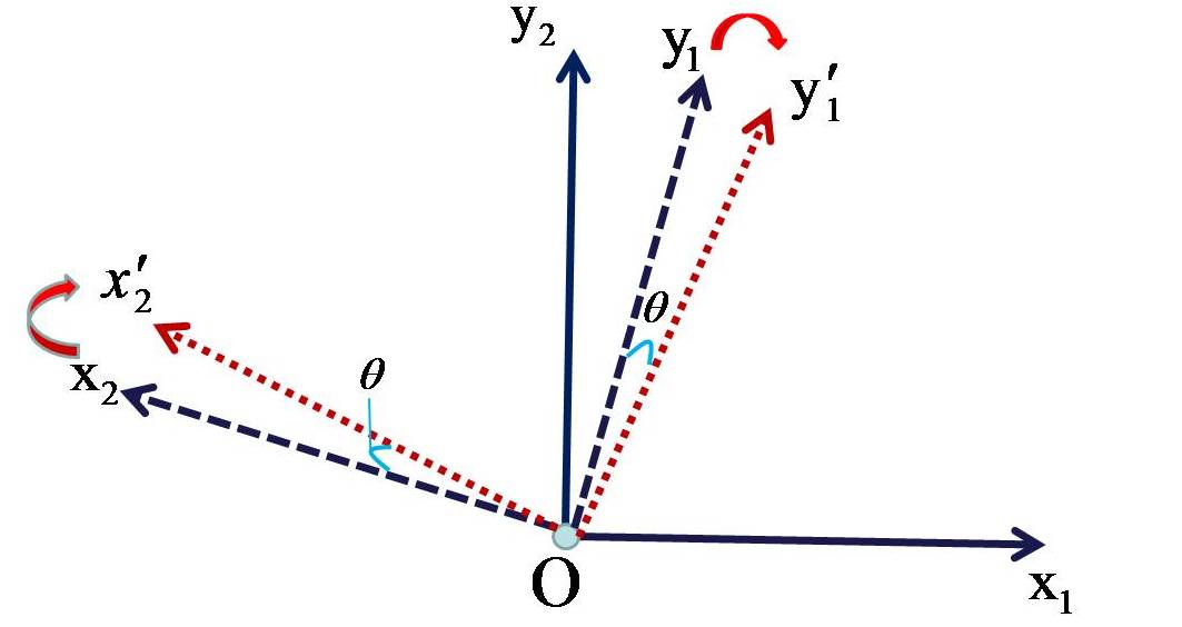
Figure 5:

The second question is: will the angle $\alpha_{j}^{\prime}=\angle(x_{j},y_{j}^{\prime})$ still be larger than, say, $\frac{1}{3}\pi$, for all $j>i$? If yes, then we can apply Operation 2 repeatedly for all $i=1,2,\dots,s$. To provide an affirmative answer, we should guarantee that each angle decreases at most $\frac{1}{s}(\frac{3}{8}\pi-\frac{1}{3}\pi)=\frac{1}{24s}\pi$, i.e. $\angle(x_{j},y_{j}^{\prime})\geq\angle(x_{j},y_{j})-\frac{1}{24s}\pi,\forall\ i<j\leq s$. Unlike the first question which can be answered by reading Figure 6 and Figure 7, this question cannot be answered by just reading figures. We make some algebraic computation to obtain the following result: under the assumption that $\alpha_{i}$ is no less than $\alpha_{j}$, during Operation 2 the amount of decrease in $\alpha_{j}$ is upper bounded by the amount of decrease in $\alpha_{i}$, which can be further bounded above by $\frac{1}{24s}\pi$. This result explains why our proof requires the assumption $\alpha_{i}\geq\alpha_{j},\forall\ i<j\leq s$, i.e. (145).

C.4.2 Formal proof of Claim (C.2)

We first show how to define $x_{i}^{\prime}$ and $y_{i}^{\prime}$. Note that

$$\|x_{i}\|\|y_{i}\|=\frac{\langle x_{i},y_{i}\rangle}{\cos\alpha_{i}}\geq\frac{\Sigma_{i}}{\cos(\frac{\pi}{3})}=2\Sigma_{i}.$$ (170)

Since (170) implies $\frac{\Sigma_{i}+D_{i}}{\|x_{i}\|\|y_{i}\|}\leq\frac{2\Sigma_{i}}{\|x_{i}\|\|y_{i}\|}\leq 1$, we can define

$$\alpha_{i}^{\prime}\triangleq\arccos(\frac{\Sigma_{i}+D_{i}}{\|x_{i}\|\|y_{i}\|})\in[0,\frac{\pi}{2}].$$

There is a unique $x_{i}^{\prime}$ in the plane $\mathrm{span}\{x_{i},y_{i}\}$ which satisfies

$$\|x_{i}^{\prime}\|=\|x_{i}\|$$ (171)

and $\angle(x_{i}^{\prime},y_{i})=\alpha_{i}^{\prime}$. By the definition of $\alpha_{i}^{\prime}$ above, we have

$$\langle x_{i}^{\prime},y_{i}\rangle=\Sigma_{i}+D_{i}.$$

The existence of $x_{i}^{\prime}$ is proved. We define

$$y_{i}^{\prime}\triangleq\frac{\Sigma_{i}}{\Sigma_{i}+D_{i}}y_{i},$$ (172)

then

$$\langle x_{i}^{\prime},y_{i}^{\prime}\rangle=\frac{\Sigma_{i}}{\Sigma_{i}+D_{i}}\langle x_{i}^{\prime},y_{i}\rangle=\Sigma_{i}.$$ (173)

The existence of $y_{i}^{\prime}$ is also proved.

Since $0<\langle x_{i},y_{i}\rangle=\Sigma_{i}<\langle x_{i}^{\prime},y_{i}\rangle$, we have $\frac{\pi}{2}>\alpha_{i}>\alpha_{i}^{\prime}>0,$ thus we can define

$$\theta\triangleq\alpha_{i}-\alpha_{i}^{\prime}=\angle(x_{i}^{\prime},x_{i})\in(0,\alpha_{i}).$$ (174)

Fix any $j\neq i$, we then show how to define $y_{j}^{\prime}.$ Define

$$A_{i}\triangleq\mathrm{span}_{j\neq i}\{x_{j}\}\bot y_{i},\;\;B_{i}\triangleq\mathrm{span}_{j\neq i}\{y_{j}\}\bot x_{i},\;\;T_{i}\triangleq A_{i}\cap B_{i}.$$

Let $\overrightarrow{OY_{j}}=y_{j}$, $K_{j}\triangleq\mathcal{P}_{A_{i}}(Y_{j}),H_{j}\triangleq\mathcal{P}_{T_{i}}(Y_{j}).$ Then $\angle Y_{j}H_{j}K_{j}=\min\{\angle(x_{i},y_{i}),\pi-\angle(x_{i},y_{i})\}=\angle(x_{i},y_{i})=\alpha_{i}.$ Since $\alpha_{i}>\theta$, there exists a unique point $Y_{j}^{\prime}$ in the line segment $Y_{j}K_{j}$ such that

$$\angle Y_{j}H_{j}Y_{j}^{\prime}=\theta.$$ (175)

Since $K_{j}=\mathcal{P}_{A_{i}}(Y_{j})$ and $x_{k}\in A_{i},\forall k\neq i$, we have $\overrightarrow{Y_{j}K_{j}}\bot x_{k},\forall k\neq i$, thus

$$\overrightarrow{Y_{j}Y_{j}^{\prime}}\bot x_{k},\;\;\forall k\neq i.$$ (176)

See Figure 6 and Figure 7 for the geometrical interpretation; note that $T_{i}$ in general is not a line but a $r-2$ dimensional space. The righthand side subfigures represents the 2 dimensional subspace $T_{i}^{\bot}$; since $\mathrm{span}\{H_{j}Y_{j},H_{j}K_{j}\}=T_{i}^{\bot}=\mathrm{span}\{x_{i},y_{i}\},$ we can draw $x_{i},y_{i},y_{i}^{\prime}$ as the vectors starting from $H_{j}$ and lying in the plane $H_{j}Y_{j}K_{j}=T_{i}^{\bot}$ in the figures. Figure 6 and Figure 7 differ in the relative position of $x_{i}$ and $K_{j}$: $x_{i}$ and $K_{j}$ lie in the same side of line $H_{j}Y_{j}$ in Figure 6 but in different sides in Figure 7. Given the positions of $x_{i}$ and $H_{j},Y_{j},K_{j}$, the position of $y_{i}$ is determined since $y_{i}\bot\overrightarrow{H_{j}K_{j}}$ and $\angle(x_{i},y_{i})<\frac{\pi}{2}$.

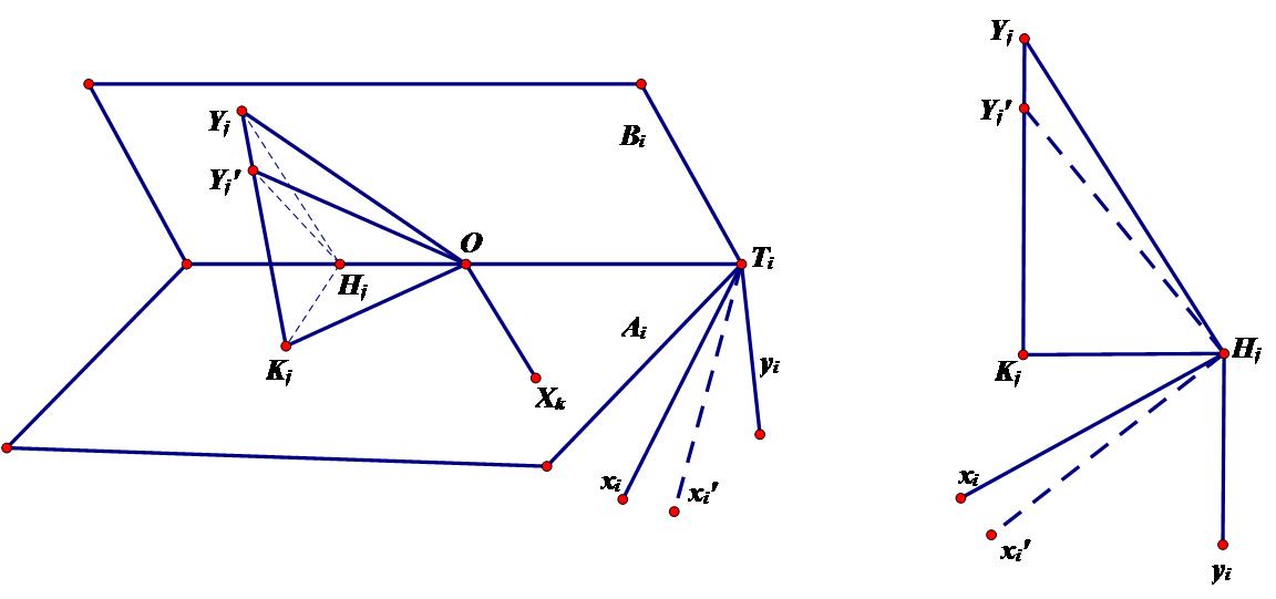
Figure 6: Left: Space $A_{i},B_{i},T_{i}$, vectors $x_{i},y_{i},x_{i}^{\prime},x_{k}$ and some points related to $y_{j}$. Right: Some points and vectors in plane $H_{j}Y_{j}K_{j}=T_{i}^{\bot}=\mathrm{span}\{x_{i},y_{i}\}$. This figure shows the first possibility: $x_{i}$ and $K_{j}$ lie in the same side of line $H_{j}Y_{j}$.

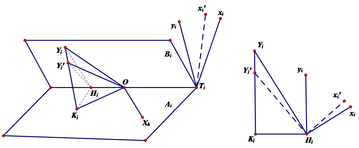
Figure 7: Same objects as in Figure 6, but for the second possibility: $x_{i}$ and $K_{j}$ lie in different sides of line $H_{j}Y_{j}$.

In both figures, we have

$$\angle(\overrightarrow{H_{j}Y_{j}^{\prime}},x_{i}^{\prime})=\angle(\overrightarrow{H_{j}Y_{j}},x_{i})-\angle(x_{i}^{\prime},x_{i})+\angle Y_{j}H_{j}Y_{j}^{\prime}$$

$$\xlongequal{\eqref{theta definition},\eqref{Y_j' position with angle theta}}\frac{\pi}{2}-\theta+\theta=\frac{\pi}{2},$$

$$\Longrightarrow \quad\quad\overrightarrow{H_{j}Y_{j}^{\prime}}\bot x_{i}^{\prime}.$$ (177)

Now we are ready to define $y_{j}^{\prime}$ and establish its properties. Define

$$\begin{split}y_{j}^{\prime}\triangleq\overrightarrow{OY_{j}^{\prime}}.\end{split}$$ (178)

Since $Y_{j}^{\prime}$ lies in the line segment $K_{j}Y_{j}$ and $\angle Y_{j}K_{j}O=\pi/2$, we have

$$\|y_{j}^{\prime}\|\leq\|y_{j}\|.$$ (179)

We also have

$$y_{j}^{\prime}=y_{j}+\overrightarrow{Y_{j}Y_{j}^{\prime}}\in\mathrm{span}\{y_{j},y_{i}\}\;\bot x_{k},\;\forall k\neq i,j.$$ (180)

According to the fact $\overrightarrow{OH_{j}}\bot x_{i}^{\prime}$ and (177), we have

$$y_{j}^{\prime}=\overrightarrow{OH_{j}}+\overrightarrow{H_{j}Y_{j}^{\prime}}\;\bot\;x_{i}^{\prime}.$$ (181)

Let $k=j$ in (176), we obtain

$$0=\langle\overrightarrow{Y_{j}Y_{j}^{\prime}},x_{j}\rangle=\langle y_{j}^{\prime}-y_{j},x_{j}\rangle=0\Longrightarrow\langle x_{j},y_{j}^{\prime}\rangle=\langle x_{j},y_{j}\rangle.$$ (182)

We have shown that $y_{j}^{\prime}$ defined in (178) satisfies (180), (181) and (182), thus the existence of $y_{j}^{\prime}$ in Operation 2 is proved.

Having defined $x_{i}^{\prime},y_{i}^{\prime}$ and $y_{j}^{\prime},\forall j\neq i$, we further define

$$x_{j}^{\prime}\triangleq x_{j},\forall j\neq i,$$ (183)

which completes the definition of $X^{\prime},Y^{\prime}$. In the rest, we prove that $X^{\prime},Y^{\prime}$ satisfy the desired property (169).

The property (169a) can be directly proved by the definitions of $X^{\prime},Y^{\prime}$. In specific, according to (173), (182) and the definition (183), we have $\langle x_{k}^{\prime},y_{k}^{\prime}\rangle=\Sigma_{k},\forall k$. According to the definitions (183), (172) and the fact $y_{i}\bot x_{j},\forall j\neq i$, we have $y_{i}^{\prime}\bot x_{j}^{\prime},\forall j\neq i$. Together with (180) and (181), we obtain $\langle x_{k}^{\prime},y_{l}^{\prime}\rangle=0,\forall k\neq l$. Thus $X^{\prime}(Y^{\prime})^{T}=\Sigma.$

Next, we prove the property (169d). We first prove

$$\alpha_{i}^{\prime}-\alpha_{i}=\theta\leq\frac{1}{r}\frac{\pi}{24}.$$ (184)

Define $h_{i}\triangleq x_{i}^{\prime}-x_{i},$ then

$$\|h_{i}\|=2\|x_{i}\|\sin(\frac{\theta}{2}).$$ (185)

From $\langle x_{i}^{\prime},y_{i}\rangle=\Sigma_{i}+D_{i}=\langle x_{i},y_{i}\rangle+D_{i},$ we obtain $\langle h_{i},y_{i}\rangle=D_{i}.$ Note that $\langle h_{i},y_{i}\rangle=\|h_{i}\|\|y_{i}\|\cos(\angle(h_{i},y_{i}))$ and $\angle(h_{i},y_{i})=\frac{\pi}{2}-\alpha_{i}+\frac{\theta}{2},$ thus

$$\|h_{i}\|=\frac{D_{i}}{\|y_{i}\|\sin(\alpha_{i}-\frac{\theta}{2})}.$$ (186)

According to (185) and (186), we have

$$\frac{D_{i}}{\|x_{i}\|\|y_{i}\|}=2\sin(\alpha_{i}-\frac{\theta}{2})\sin(\frac{\theta}{2})\geq 2\sin(\frac{\alpha_{i}}{2})\sin(\frac{\theta}{2})$$

$$\geq 2\sin(\frac{\pi}{6})\sin(\frac{\theta}{2})=\sin(\frac{\theta}{2})\geq\frac{\theta}{\pi},$$

where the last equality follows from the fact that $\frac{\sin(t)}{t}$ is decreasing in $t\in(0,\frac{\pi}{2}]$. Note that $\frac{D_{i}}{\|x_{i}\|\|y_{i}\|}$ can be upper bounded as

$$\frac{D_{i}}{\|x_{i}\|\|y_{i}\|}\overset{\eqref{x_i y_i bound}}{\leq}\frac{D_{i}}{2\Sigma_{i}}\overset{\eqref{D_i bound by Sigma_i/10}}{\leq}\frac{1}{24r}.$$

Combining the above two relations, we get (184).

To prove

$$\alpha_{j}-\alpha_{j}^{\prime}\leq\frac{\pi}{24r},\forall j\in\{i+1,\dots,s\},$$ (187)

we only need to prove

$$\theta_{j}\triangleq\alpha_{j}-\alpha_{j}^{\prime}\leq\theta,\;\;\forall j\in\{i+1,\dots,s\}$$ (188)

and then use (184). The equality (182) implies that $\|x_{j}\|\|y_{j}\|\cos(\alpha_{j})=\|x_{j}\|\|y_{j}^{\prime}\|\cos(\alpha_{j}^{\prime})$, which leads to

$$\frac{\cos(\alpha_{j})}{\cos(\alpha_{j}-\theta_{j})}=\frac{\cos(\alpha_{j})}{\cos(\alpha_{j}^{\prime})}=\frac{\|y_{j}^{\prime}\|}{\|y_{j}\|}.$$

For any two points $P_{1},P_{2}$, we use $|P_{1}P_{2}|$ to denote the length of the line segment $P_{1}P_{2}$. Since $\overrightarrow{OH_{j}}$ is orthogonal to plane $H_{j}K_{j}Y_{j}$, we have

$$\frac{\|y_{j}^{\prime}\|^{2}}{\|y_{j}\|^{2}}=\frac{|OH_{j}|^{2}+|H_{j}Y_{j}^{\prime}|^{2}}{|OH_{j}|^{2}+|H_{j}Y_{j}|^{2}}\geq\frac{|H_{j}Y_{j}^{\prime}|^{2}}{|H_{j}Y_{j}|^{2}},$$

where the last inequality follows from the fact that $|H_{j}Y_{j}^{\prime}|\leq|H_{j}Y_{j}|$. Since $\angle Y_{j}H_{j}K_{j}=\alpha_{i},\angle Y_{j}^{\prime}H_{j}K_{j}=\alpha_{i}^{\prime}$ and $\angle Y_{j}K_{j}H_{j}=\frac{\pi}{2}$, we have

$$\frac{|H_{j}Y_{j}^{\prime}|}{|H_{j}Y_{j}|}=\frac{\sin\angle Y_{j}^{\prime}Y_{j}H_{j}}{\sin\angle Y_{j}Y_{j}^{\prime}H_{j}}=\frac{\sin(\pi/2-\alpha_{i})}{\sin(\pi/2+\alpha_{i}^{\prime})}=\frac{\cos(\alpha_{i})}{\cos(\alpha_{i}^{\prime})}.$$

According to the assumption (145) and $i<j\leq s$, we have $0\leq\alpha_{i}\leq\alpha_{j}\leq\frac{\pi}{2}$. Since $\cos(x)/\cos(x-\theta)$ is decreasing in $[0,\frac{\pi}{2}]$, we can get

$$\frac{\cos(\alpha_{i})}{\cos(\alpha_{i}^{\prime})}=\frac{\cos(\alpha_{i})}{\cos(\alpha_{i}-\theta)}\geq\frac{\cos(\alpha_{j})}{\cos(\alpha_{j}-\theta)}.$$

Combining the above four relations, we get

$$\frac{\cos(\alpha_{j})}{\cos(\alpha_{j}-\theta_{j})}\geq\frac{\cos(\alpha_{j})}{\cos(\alpha_{j}-\theta)},$$

which implies $\cos(\alpha_{j}-\theta)\geq\cos(\alpha_{j}-\theta_{j})$ that immediately leads to (188). Thus we have proved (187), which combined with (184) establishes the property (169d).

Then we prove the property (169c). Since $x_{j}^{\prime}=x_{j},\forall j\neq i$, we have $\|X^{\prime}-X\|_{F}=\|x_{i}^{\prime}-x_{i}\|$, which can be bounded as

$$\|x_{i}^{\prime}-x_{i}\|=\|h_{i}\|\overset{\eqref{h_i expression 2}}{=}\frac{D_{i}}{\|y_{i}\|\sin(\alpha_{i}-\frac{\theta}{2})}\leq\frac{\|x_{i}\|D_{i}}{\|x_{i}\|\|y_{i}\|\sin(\frac{\pi}{3})}$$

$$\overset{\eqref{x_i y_i bound}}{\leq}\frac{\|x_{i}\|D_{i}}{2\Sigma_{i}\sin(\frac{\pi}{3})}<\frac{1}{\sqrt{3}}\frac{\|x_{i}\|}{\Sigma_{i}}D_{i},$$

where the first inequality is due to

$$\alpha_{i}-\theta/2\geq\alpha_{i}-\theta\overset{\eqref{alpha_i bound, Claim 3}}{\geq}\pi/3+\pi/24-\theta\overset{\eqref{theta bound we want}}{\geq}\pi/3.$$ (189)

Thus the first part of (169c) is proved.

According to (185) and (186), we have

$$2\sin(\frac{\theta}{2})=\frac{D_{i}}{\|x_{i}\|\|y_{i}\|\sin(\alpha_{i}-\frac{\theta}{2})}$$ (190)

Now we upper bound $\|y_{j}^{\prime}-y_{j}\|$ as

$$\begin{split}&\|y_{j}^{\prime}-y_{j}\|=|Y_{j}^{\prime}Y_{j}|\\ &=\frac{\sin(\theta)}{\cos(\alpha_{i}-\theta)}|H_{j}Y_{j}|\\ &=2\sin(\frac{\theta}{2})\cos(\frac{\theta}{2})\frac{1}{\cos(\alpha_{i}-\theta)}|H_{j}Y_{j}|\\ &\overset{\eqref{sin theta/2 expression}}{=}\frac{D_{i}}{\|x_{i}\|\|y_{i}\|\sin(\alpha_{i}-\frac{\theta}{2})}\cos(\frac{\theta}{2})\frac{1}{\cos(\alpha_{i}-\theta)}|H_{j}Y_{j}|\\ &\leq\frac{D_{i}}{\|x_{i}\|\|y_{i}\|\sin(\alpha_{i}-\frac{\theta}{2})}\frac{1}{\cos(\alpha_{i})}|H_{j}Y_{j}|\\ &\overset{\eqref{alpha - theta bound}}{\leq}\frac{D_{i}}{\sin(\frac{\pi}{3})\langle x_{i},y_{i}\rangle}|H_{j}Y_{j}|\\ &\leq\frac{2}{\sqrt{3}}\frac{D_{i}}{\Sigma_{i}}|H_{j}Y_{j}|,\end{split}$$ (191)

where the last inequality is due to the fact $\langle x_{i},y_{i}\rangle=\Sigma_{i}$. Using $|H_{j}Y_{j}|\leq\|y_{j}\|$, we obtain

$$\|y_{j}^{\prime}-y_{j}\|\leq\frac{2}{\sqrt{3}}\frac{D_{i}}{\Sigma_{i}}\|y_{j}\|.$$ (192)

According to the definition (172), we have

$$\|y_{i}-y_{i}^{\prime}\|=(1-\frac{\Sigma_{i}}{\Sigma_{i}+D_{i}})\|y_{i}\|=\frac{D_{i}}{\Sigma_{i}+D_{i}}\|y_{i}\|\leq\frac{D_{i}}{\Sigma_{i}}\|y_{i}\|.$$ (193)

According to (192) (which holds for any $j\in\{1,\dots,r\}\backslash\{i\}$) and (193), we get

$$\|Y-Y^{\prime}\|_{F}=\sqrt{\sum_{k=1}^{r}\|y_{k}-y_{k}^{\prime}\|^{2}}\leq\frac{2}{\sqrt{3}}\frac{D_{i}}{\Sigma_{i}}\sqrt{\sum_{k=1}^{r}\|y_{k}\|^{2}}=\frac{2}{\sqrt{3}}\frac{D_{i}}{\Sigma_{i}}\|Y\|_{F},$$

which proves the second part of (169c).

The property (169e) can be proved as follows. By the definition (172), we have $\|y_{i}^{\prime}\|\leq\|y_{i}\|$, which combined with (179) (for all $j\neq i$) leads to

$$\|y_{k}^{\prime}\|\leq\|y_{k}\|,\;\;k=1,\dots,s.$$

According to (192) (for all $j\neq i$) and (193), we have $\|y_{k}^{\prime}-y_{k}\|\leq\frac{2}{\sqrt{3}}\frac{D_{i}}{\Sigma_{i}}\|y_{k}\|,\forall k$, which implies

$$\|y_{k}^{\prime}\|\geq\|y_{k}\|-\|y_{k}^{\prime}-y_{k}\|\geq\|y_{k}\|-\frac{2}{\sqrt{3}}\frac{D_{i}}{\Sigma_{i}}\|y_{k}\|\overset{\eqref{D_i bound by Sigma_i/10}}{\geq}\|y_{k}\|-\frac{1}{10r}\|y_{k}\|,\;\forall k.$$

Combining the above two relations we obtain the property (169e).

The property (169f) can be easily proved by (172). In fact, we have

$$\begin{split}\|y_{i}\|^{2}-\|y_{i}^{\prime}\|^{2}=(\|y_{i}\|-\|y_{i}^{\prime}\|)(\|y_{i}\|+\|y_{i}^{\prime}\|)\\ \geq 2\|y_{i}^{\prime}\|(\|y_{i}\|-\|y_{i}^{\prime}\|)\overset{\eqref{y_i prime def}}{=}2\|y_{i}^{\prime}\|(\frac{\Sigma_{i}+D_{i}}{\Sigma_{i}}-1)\|y_{i}^{\prime}\|\\ =2\frac{D_{i}}{\Sigma_{i}}\|y_{i}^{\prime}\|^{2}\geq 2\frac{D_{i}}{\Sigma_{i}}(\frac{11}{12})^{2}\|y_{i}\|^{2}\geq\frac{5}{3}\frac{D_{i}}{\Sigma_{i}}\|y_{i}\|^{2}.\end{split}$$ (194)

where the second last inequliaty follows from $\|y_{i}^{\prime}\|\geq\|y_{i}\|-\|y_{i}-y_{i}^{\prime}\|\overset{\eqref{y_i diff bound}}{\geq}\|y_{i}\|-D_{i}\|y_{i}\|/\Sigma_{i}\overset{\eqref{D_i bound by Sigma_i/10}}{\geq}11\|y_{i}\|/12.$ According to (179) (for all $j\neq i$), we have $\|Y\|_{F}^{2}-\|Y^{\prime}\|_{F}^{2}\geq\|y_{i}\|^{2}-\|y_{i}^{\prime}\|^{2}$, which combined with (194) leads to the property (169f).

At last, we prove the property (169b). The first part $\|X^{\prime}\|_{F}=\|X\|_{F}$ follows from (171) and (183), thus it remains to prove the second part. Denote $\varphi_{j}\triangleq\angle Y_{j}OY_{j}^{\prime},\beta_{j}\triangleq\angle Y_{j}OK_{j}$ as shown in Figure 8.

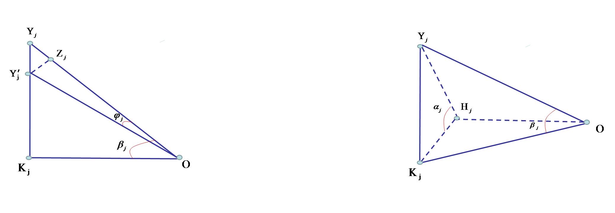
Figure 8: Illustration for the proof of the property (169b)

Pick a point $Z_{j}$ in the line segment $OY_{j}$ so that $|OZ_{j}|=|OY_{j}^{\prime}|$, then $|Y_{j}Z_{j}|=\|y_{j}\|-\|y_{j}^{\prime}\|$. Thus we have

$$\begin{split}\frac{\|y_{j}-y_{j}^{\prime}\|}{\|y_{j}\|-\|y_{j}^{\prime}\|}=\frac{|Y_{j}Y_{j}^{\prime}|}{|Y_{j}Z_{j}|}=\frac{\sin(\angle Y_{j}Z_{j}Y_{j}^{\prime})}{\sin(\angle Y_{j}Y_{j}^{\prime}Z_{j})}\\ =\frac{\sin(\pi/2-\varphi_{j}/2)}{\sin(\beta_{j}-\varphi_{j}/2)}\leq\frac{1}{\sin(\beta_{j}-\varphi_{j})}.\end{split}$$ (195)

In order to bound $1/\sin(\beta_{j}-\varphi_{j})$ , we use the following bound:

$$\frac{\sin\beta_{j}}{\sin(\beta_{j}-\varphi_{j})}=\frac{|Y_{j}K_{j}|}{\|y_{j}\|}\frac{\|y_{j}^{\prime}\|}{|Y_{j}^{\prime}K_{j}|}\leq\frac{|Y_{j}K_{j}|}{|Y_{j}^{\prime}K_{j}|}=\frac{\tan\alpha_{i}}{\tan(\alpha_{i}-\theta)}.$$

Then we have

$$\begin{split}\frac{\sin\beta_{j}}{\sin(\beta_{j}-\varphi_{j})}\frac{\sin(\alpha_{i}-\theta)}{\sin(\alpha_{i})}\frac{\cos(\alpha_{i}-\theta)}{\cos(\alpha_{i})}\\ =\frac{\cos\alpha_{i}\cos\theta+\sin\alpha_{i}\sin\theta}{\cos(\alpha_{i})}\leq\frac{\sin(\theta)}{\cos(\alpha_{i})}+1.\end{split}$$ (196)

According to (190) and the fact $\cos(\alpha_{i})=\langle x_{i},y_{i}\rangle/(\|x_{i}\|\|y_{i}\|)=\Sigma_{i}/(\|x_{i}\|\|y_{i}\|)$, we have

$$\begin{split}\frac{\sin(\theta)}{\cos(\alpha_{i})}\leq\frac{2\sin(\theta/2)}{\cos(\alpha_{i})}=\frac{D_{i}}{\|x_{i}\|\|y_{i}\|\sin(\alpha_{i}-\theta/2)}\frac{\|x_{i}\|\|y_{i}\|}{\Sigma_{i}}\\ =\frac{D_{i}}{\Sigma_{i}}\frac{1}{\sin(\alpha_{i}-\theta/2)}\overset{\eqref{D_i bound by Sigma_i/10},\eqref{alpha - theta bound}}{\leq}\frac{1}{12}\frac{1}{\sin(\pi/3)}=\frac{1}{6\sqrt{3}}.\end{split}$$

Plugging the above relation into (196), we obtain

$$\frac{\sin\beta_{j}}{\sin(\beta_{j}-\varphi_{j})}\frac{\sin(\alpha_{i}-\theta)}{\sin(\alpha_{i})}\leq\frac{6\sqrt{3}+1}{6\sqrt{3}}.$$ (197)

Combining (195) and (191), we obtain

$$\begin{split}&\frac{\|y_{j}-y_{j}^{\prime}\|}{\|y_{j}\|-\|y_{j}^{\prime}\|}\frac{\|y_{j}-y_{j}^{\prime}\|}{\|y_{j}\|}\\ &\leq\frac{1}{\sin(\beta_{j}-\varphi_{j})}\frac{2}{\sqrt{3}}\frac{D_{i}}{\Sigma_{i}}\frac{|H_{j}Y_{j}|}{\|y_{j}\|}\\ &\overset{\eqref{sin(beta) bound}}{\leq}\frac{2}{\sqrt{3}}\frac{D_{i}}{\Sigma_{i}}\frac{6\sqrt{3}+1}{6\sqrt{3}}\frac{|H_{j}Y_{j}|}{\|y_{j}\|}\frac{\sin(\alpha_{i})}{\sin(\beta_{j})}\frac{1}{\sin(\alpha_{i}-\theta)}\\ &=\frac{6\sqrt{3}+1}{9}\frac{D_{i}}{\Sigma_{i}}\frac{1}{\sin(\alpha_{i}-\theta)}\overset{\eqref{alpha - theta bound}}{\leq}\frac{6\sqrt{3}+1}{9}\frac{2}{\sqrt{3}}\frac{D_{i}}{\Sigma_{i}}\leq\frac{3}{2}\frac{D_{i}}{\Sigma_{i}},\end{split}$$ (198)

where the last equality is due to $|H_{j}Y_{j}|\sin(\alpha_{i})=|Y_{j}K_{j}|=\|y_{j}\|\sin(\beta_{j})$.

According to (192) and (146), we obtain that $\|y_{j}-y_{j}^{\prime}\|\leq\frac{2}{\sqrt{3}}\frac{1}{12}\|y_{j}\|\leq\frac{1}{8}\|y_{j}\|$, which further implies $\|y_{j}^{\prime}\|+\|y_{j}\|\geq 2\|y_{j}\|-\|y_{j}-y_{j}^{\prime}\|\geq\frac{15}{8}\|y_{j}\|$. Then by (198) we have

$$\begin{split}\|y_{j}-y_{j}^{\prime}\|^{2}\leq\frac{5\sqrt{3}+1}{6}\frac{D_{i}}{\Sigma_{i}}(\|y_{j}\|-\|y_{j}^{\prime}\|)\|y_{j}\|\\ \leq\frac{3}{2}\frac{D_{i}}{\Sigma_{i}}(\|y_{j}\|-\|y_{j}^{\prime}\|)(\|y_{j}^{\prime}\|+\|y_{j}\|)\frac{8}{15}=\frac{4}{5}\frac{D_{i}}{\Sigma_{i}}(\|y_{j}\|^{2}-\|y_{j}^{\prime}\|^{2}).\end{split}$$ (199)

According to the definition (172), we have

$$\frac{\|y_{i}\|^{2}-\|y_{i}^{\prime}\|^{2}}{\|y_{i}-y_{i}^{\prime}\|^{2}}=\frac{1-(\Sigma_{i})^{2}/(\Sigma_{i}+D_{i})^{2}}{[1-\Sigma_{i}/(\Sigma_{i}+D_{i})]^{2}}$$

$$=\frac{(\Sigma_{i}+D_{i})^{2}-\Sigma_{i}^{2}}{D_{i}^{2}}=\frac{D_{i}^{2}+2D_{i}\Sigma_{i}}{D_{i}^{2}}\geq 2\frac{\Sigma_{i}}{D_{i}},$$

which implies

$$\|y_{i}-y_{i}^{\prime}\|^{2}\leq\frac{1}{2}\frac{D_{i}}{\Sigma_{i}}(\|y_{i}\|^{2}-\|y_{i}^{\prime}\|^{2}).$$ (200)

Summing up (199) for $j\in\{1,\dots,r\}\backslash\{i\}$ and (200), we obtain

$$\|Y-Y^{\prime}\|_{F}^{2}\leq\frac{4}{5}\frac{D_{i}}{\Sigma_{i}}(\|Y\|_{F}^{2}-\|Y^{\prime}\|_{F}^{2}),$$

which proves the second part of (169b).

Appendix D Proofs of the results in Section 5

D.1 Proof of Claim 5.2

The proof of this claim consists of two parts: first, by a classical result we have that $M_{0}$, the best rank-$r$ approximation of $\frac{1}{p}\mathcal{P}_{\Omega}(M)$, is close to $M$; second, show that the scaling does not change the closeness.

We first present the following result.

Lemma D.1

Assume $M$ is a rank $r$ matrix of dimension $m\times n$ with $m\geq n$, and denote $M_{\max}=\|M\|_{\infty}$ as the maximum magnitude of the entries of $M$. Suppose each entry of $M$ is included in $\Omega$ with probability $p\geq C_{0}\frac{\log(m+n)}{m}$, and $M_{0}$ is the best rank-r approximation of $\frac{1}{p}\mathcal{P}_{\Omega}(M)$. Then with probability larger than $1-1/(2n^{4})$,

$$\frac{1}{mnM_{\max}^{2}}\|M-M_{0}\|_{F}^{2}\leq C_{2}\frac{\alpha^{\frac{3}{2}}{r}}{pm},$$ (201)

for some numerical constant $C_{2}$.

Remark: Lemma D.1 can be found in [31]. The original version [31, Theorem 1.1] holds for $M_{0}=\mathrm{P}_{r}(\mathrm{T}_{\mathrm{r}}(\mathcal{P}_{\Omega}(M))/p)$, where $\mathrm{T}_{\mathrm{r}}(\cdot)$ denotes a trimming operator which sets to zero all rows and columns that have too many observed entries, and $\mathrm{P}_{r}(\cdot)$ denotes the best rank-$r$ approximation. By standard Chernoff bound one can show that none of the rows and columns have too many observed entries with high probability, thus the conclusion of [31, Theorem 1.1] holds for $M_{0}=\mathrm{P}_{r}(\mathcal{P}_{\Omega}(M))/p$. The key to establish Lemma D.1 is a bound on $\|M-\frac{1}{p}\mathcal{P}_{\Omega}(M)\|_{2}$, which can be simply proved by matrix concentration inequalities; see [17, Remark 6.1.2], [4, Theorem 6.3] or [7, Theorem 3.5]. The proof of [31, Theorem 1.1] is more complicated than applying matrix concentration inequalities since it holds for a weaker condition $|\Omega|\geq O(n)$.

Note that $\hat{X}_{0},\hat{Y}_{0}$ defined in Table 1 satisfy

$$\hat{X}_{0}\hat{Y_{0}}^{T}=\mathrm{P}_{r}(\mathcal{P}_{\Omega}(M)/p)=M_{0}.$$ (202)

Recall that the SVD of $M$ is $M=\hat{U}\Sigma\hat{V}$, where $\hat{U},\hat{V}$ satisfies (12). We have

$$\begin{split}|M_{ij}|=\sum_{k=1}^{r}|\hat{U}_{ik}\hat{V}_{jk}\Sigma_{k}|\leq\Sigma_{\rm max}\sum_{k=1}^{r}|\hat{U}_{ik}\hat{V}_{jk}|\\ \leq\Sigma_{\rm max}\sqrt{\sum_{k=1}^{r}\hat{U}_{ik}^{2}}\sqrt{\sum_{k=1}^{r}\hat{V}_{jk}^{2}}\overset{\eqref{incoherence cond}}{\leq}\Sigma_{\rm max}\frac{\mu r}{\sqrt{mn}},\ \forall\ i,j.\end{split}$$ (203)

The above relation implies $M_{\rm max}\leq\Sigma_{\rm max}\frac{\mu r}{\sqrt{mn}}$. Plugging this inequality and $p=|\Omega|/(mn)$ into (201), we get

$$\|M-M_{0}\|_{F}^{2}\leq C_{2}\frac{mn\alpha^{\frac{3}{2}}r}{pm}\Sigma_{\rm max}^{2}\frac{\mu^{2}r^{2}}{mn}=C_{2}n\frac{\alpha^{\frac{3}{2}}r^{3}\kappa^{2}\mu^{2}}{|\Omega|}\Sigma_{\rm min}^{2}.$$ (204)

Plugging (202) and the assumption (27) into (204), we get

$$\hat{\delta}_{0}\triangleq\|M-\hat{X}_{0}\hat{Y_{0}}^{T}\|_{F}\leq\sqrt{\frac{C_{2}}{C_{0}}}\frac{\Sigma_{\min}}{r^{1.5}\kappa^{2}}.$$ (205)

The property (a), i.e. $(X_{0},Y_{0})\in(\sqrt{2/3}K_{1})$ follows directly from the definitions of $X_{0}$ and $Y_{0}$ in (23). We then prove the property (b), i.e. $(X_{0},Y_{0})\in(\sqrt{2/3}K_{2})$. By (205) we have $\|M-M_{0}\|_{F}\leq\Sigma_{\rm min}/5\leq\Sigma_{\rm max}/5$ for large enough $C_{0}$. This inequality combined with $\|M-M_{0}\|_{F}\geq\|M-M_{0}\|_{2}\geq\|M_{0}\|_{2}-\Sigma_{\rm max}$ yields

$$\|M_{0}\|_{2}\leq\frac{6}{5}\Sigma_{\rm max}.$$ (206)

By the definitions of $\hat{X}_{0},\hat{Y}_{0}$ (i.e. $\hat{X}_{0}=\bar{X}_{0}D_{0}^{\frac{1}{2}}$, $\hat{Y}_{0}=\bar{Y}_{0}D_{0}^{\frac{1}{2}}$, where $\bar{X}_{0}D_{0}\bar{Y}_{0}^{T}$ is the SVD of $M_{0}$), we have

$$\|\hat{X}_{0}\|_{2}=\|\hat{Y}_{0}\|_{2}=\sqrt{\|M_{0}\|_{2}}\overset{\eqref{M_0 spectral bound}}{\leq}\sqrt{\frac{6}{5}}\sqrt{\Sigma_{\rm max}}.$$ (207)

Then we have

$$\|\hat{X}_{0}\|_{F}^{2}\leq r\|\hat{X}_{0}\|_{2}^{2}\leq\frac{6}{5}r\Sigma_{\rm max}\overset{\eqref{beta 1 beta T def}}{<}\frac{2}{3}\beta_{T}^{2},$$ (208)

where the last inequality follows from $C_{T}>9/5.$ By the definition of $X_{0}$ in (23), we have $\|X_{0}\|_{F}^{2}\leq\|\hat{X}_{0}\|_{F}^{2}\leq\frac{2}{3}\beta_{T}^{2}$. Similarly, we can prove $\|Y_{0}\|_{F}^{2}\leq\frac{2}{3}\beta_{T}^{2}$. Thus the property (b) is proved.

Next we prove the property (c), i.e. $\|M-X_{0}Y_{0}^{T}\|_{F}\leq\delta_{0}$. Since $\hat{X}_{0},\hat{Y}_{0}$ satisfy $\max\{\|\hat{X}_{0}\|_{F},\|\hat{Y}_{0}\|_{F}\}\leq\beta_{T}$ (due to (208) and the analogous inequality for $\hat{Y}_{0}$) and (205), it follows from Proposition 4.1 that there exist $U_{0},V_{0}$ such that

$$U_{0}V_{0}^{T} =M;$$ (209a)

$$\|U_{0}\|_{2} \leq\|X_{0}\|_{2};$$ (209b)

$$\|U_{0}-\hat{X}_{0}\|_{F}\leq\frac{6\|\hat{Y}_{0}\|_{2}}{5\Sigma_{\min}}\hat{\delta}_{0}, \;\;\|V_{0}-\hat{Y}_{0}\|_{F}\leq\frac{3\|\hat{X}_{0}\|_{2}}{\Sigma_{\min}}\hat{\delta}_{0};$$ (209c)

$$\|U_{0}^{(i)}\|^{2}\leq\frac{r\mu}{m}\beta_{T}^{2}, \;\;\|V_{0}^{(j)}\|^{2}\leq\frac{3r\mu}{2n}\beta_{T}^{2}.$$ (209d)

Note that the above inequalities (209b) and (209c) are not due to (48b) and (48c) of Proposition 4.1, but stronger results (99) and (107) established during the proof of Proposition 4.1.

Note that

$$\begin{split}&\|M-X_{0}Y_{0}^{T}\|_{F}=\|U_{0}(V_{0}-Y_{0})^{T}+(U_{0}-X_{0})Y_{0}^{T}\|_{F}\\ &\leq\|U_{0}(V_{0}-Y_{0})^{T}\|_{F}+\|(U_{0}-X_{0})Y_{0}^{T}\|_{F}\\ &\leq\|U_{0}\|_{2}\|V_{0}-Y_{0}\|_{F}+\|U_{0}-X_{0}\|_{F}\|Y_{0}\|_{2},\end{split}$$ (210)

where the last inequality follows from Proposition B.4. Since $X_{0}^{(i)}$ and $\hat{X}_{0}^{(i)}$ has the same direction and $\|X_{0}^{(i)}\|\leq\|\hat{X}_{0}^{(i)}\|$, by Proposition B.3 we have

$$\|X_{0}\|_{2}\leq\|\hat{X}_{0}\|_{2}\leq\sqrt{\frac{6}{5}}\sqrt{\Sigma_{\rm max}}.$$ (211)

Combining (209b) and (211), we get

$$\|U_{0}\|_{2}\leq\sqrt{\frac{6}{5}}\sqrt{\Sigma_{\rm max}}.$$ (212)

Similar to (211), we have

$$\|Y_{0}\|_{2}\leq\sqrt{\frac{6}{5}}\sqrt{\Sigma_{\rm max}}.$$ (213)

It remains to bound $\|V_{0}-Y_{0}\|_{F}$ and $\|U_{0}-X_{0}\|_{F}.$ Let us prove the following inequality:

$$\|U_{0}^{(i)}-X_{0}^{(i)}\|\leq\|U_{0}^{(i)}-\hat{X}_{0}^{(i)}\|,\;\;\forall\ i.$$ (214)

If $\|\hat{X}_{0}^{(i)}\|\leq\sqrt{\frac{2}{3}}\beta_{1}$, then (214) becomes equality since $\hat{X}_{0}^{(i)}=X_{0}^{(i)}$. Thus we only need to consider the case $\|\hat{X}_{0}^{(i)}\|>\sqrt{\frac{2}{3}}\beta_{1}.$ In this case by the definition of $X_{0}$ in (23) we have $\|X_{0}^{(i)}\|=\sqrt{\frac{2}{3}}\beta_{1}.$ From (209d), we get

$$\|U_{0}^{(i)}\|^{2}<\frac{3}{2}\frac{r\mu}{m}\beta_{T}^{2}\leq\frac{2}{3}\beta_{1}^{2}<\|\hat{X}_{0}^{(i)}\|^{2}.$$ (215)

For simplicity, denote $u\triangleq U_{0}^{(i)},x\triangleq X_{0}^{(i)},\tau\triangleq\frac{\|\hat{X}_{0}^{(i)}\|}{\sqrt{2/3}\beta_{1}}=\frac{\|\hat{X}_{0}^{(i)}\|}{\|x\|}>1.$ Then (215) becomes $\|u\|\leq\|x\|$ and (214) becomes $\|u-x\|\leq\|u-\tau x\|$. The latter can be transformed as follows:

$$\|u-x\|\leq\|u-\tau x\| \Longleftrightarrow\|x\|^{2}-2\langle u,x\rangle\leq\tau^{2}\|x\|^{2}-2\tau\langle u,x\rangle$$

$$\Longleftrightarrow 2(\tau-1)\langle u,x\rangle\leq(\tau^{2}-1)\|x\|^{2}$$

$$\Longleftrightarrow 2\langle u,x\rangle\leq(\tau+1)\|x\|^{2}.$$ (216)

Since $\langle u,x\rangle\leq\|u\|\|x\|\leq\|x\|^{2}$ (here we use $\|u\|\leq\|x\|$ which is equivalent to (215)) and $2<\tau+1,$ the last inequality of (216) holds, which implies that $\|u-x\|\leq\|u-\tau x\|$ holds and, consequently, (214) holds.

An immediate consequence of (214) is

$$\|U_{0}-X_{0}\|_{F}\leq\|U_{0}-\hat{X}_{0}\|_{F}\overset{\eqref{U0-X0, V0-Y0 bound}}{\leq}\frac{5\|\hat{Y}_{0}\|_{2}}{4\Sigma_{\min}}\hat{\delta}_{0}\overset{\eqref{hat(X0Y0) bound}}{\leq}\frac{5}{4}\sqrt{\frac{6}{5}}\sqrt{\Sigma_{\rm max}}\frac{\hat{\delta}_{0}}{\Sigma_{\rm min}}.$$ (217)

Similarly, we have

$$\|V_{0}-Y_{0}\|_{F}\overset{\eqref{U0-X0, V0-Y0 bound}}{\leq}3\sqrt{\frac{6}{5}}\sqrt{\Sigma_{\rm max}}\frac{\hat{\delta}_{0}}{\Sigma_{\rm min}}.$$ (218)

Plugging (212), (213), (217) and (218) into (210), we get

$$\begin{split}&\|M-X_{0}Y_{0}^{T}\|_{F}\\ \leq&\sqrt{\frac{6}{5}}\sqrt{\Sigma_{\rm max}}\frac{5}{4}\sqrt{\frac{6}{5}}\sqrt{\Sigma_{\rm max}}\frac{\hat{\delta}_{0}}{\Sigma_{\rm min}}+\sqrt{\frac{6}{5}}\sqrt{\Sigma_{\rm max}}3\sqrt{\frac{6}{5}}\sqrt{\Sigma_{\rm max}}\frac{\hat{\delta}_{0}}{\Sigma_{\rm min}}\\ =&(\frac{3}{2}+\frac{18}{5})\kappa\hat{\delta}_{0}\\ \overset{\eqref{M_0 - M bounded by hat delta0}}{\leq}&\frac{51}{10}\sqrt{\frac{C_{2}}{C_{0}}}\frac{\Sigma_{\min}}{r^{1.5}\kappa}\\ \overset{\eqref{delta definition throughout}}{\leq}&\delta_{0},\end{split}$$

where the last inequality holds for $C_{d}\geq\frac{5}{153}\sqrt{\frac{C_{0}}{C_{2}}}$. Therefore property (c) is proved.

D.2 Proof of Claim 3.1

As mentioned in Section 2.1, in this proof we only need to consider the Bernolli model that $\Omega$ includes each entry of $M$ with probability $p$ and the expected size $S$ satisfies (27). Denote $d\triangleq\|M-XY^{T}\|_{F}$. Let $a=U(V-Y)^{T}+(U-X)V^{T}$, $b=(U-X)(V-Y)$, where $U,V$ are defined with the properties in Corollary 4.1.

According to (46) we have $\|\mathcal{P}_{\Omega}(a)\|_{F}^{2}\geq\frac{27}{40}pd^{2}$. According to (40a), we have $\|\mathcal{P}_{\Omega}(b)\|_{F}\leq\frac{1}{5}\sqrt{p}d$. Therefore, $\|\mathcal{P}_{\Omega}(M-XY^{T})\|_{F}=\|\mathcal{P}_{\Omega}(a-b)\|_{F}\geq\|\mathcal{P}_{\Omega}(a)\|_{F}-\|\mathcal{P}_{\Omega}(b)\|_{F}\geq\sqrt{\frac{27}{40}}\sqrt{p}d-\frac{1}{5}\sqrt{p}d\geq\frac{3}{5}\sqrt{p}d\geq\frac{1}{\sqrt{3}}\sqrt{p}d$.

According to (40b), we have $\|b\|_{F}\leq\frac{1}{10}d$. According to (45) (which is a corollary of [4, Theorem 4.1]), we have $\|\mathcal{P}_{\Omega}(a)\|_{F}^{2}\leq\frac{7}{6}p\|a\|_{F}^{2}\leq\frac{7}{6}p(\|M-XY^{T}\|_{F}+\|b\|_{F})^{2}\leq\frac{7}{6}p(1+\frac{1}{10})^{2}d^{2}\leq\frac{17}{12}pd^{2}.$ Thus, $\|\mathcal{P}_{\Omega}(a-b)\|_{F}\leq\|\mathcal{P}_{\Omega}(a)\|_{F}+\|\mathcal{P}_{\Omega}(b)\|_{F}\leq(\sqrt{\frac{17}{12}}+\frac{1}{5})\sqrt{p}d\leq\sqrt{2p}d$.     $\Box$

D.3 Proof of Proposition 5.1

We first provide a general condition for $(X,Y)\in K_{1}\cap K_{2}$ (i.e. incoherent and bounded) based on the function value $\tilde{F}(X,Y)$.

Proposition D.1

Suppose the sample set $\Omega$ satisfies (29) and $\rho=2p\delta_{0}^{2}/G_{0}(3/2)$, where $\delta_{0}$ is defined in (16). Suppose $(X_{0},Y_{0})$ satisfies (66) and

$$\tilde{F}(X,Y)\leq 2\tilde{F}(X_{0},Y_{0}).$$ (219)

Then $(X,Y)\in K_{1}\cap K_{2}$.

Proof of Proposition D.1: We prove by contradiction. Assume the contrary that $(X,Y)\notin K_{1}\cap K_{2}$. By the definition of $K_{1},K_{2}$ in (30), we have either $\|X^{(i)}\|^{2}>\beta_{1}^{2}$ for some $i$, $\|Y^{(j)}\|^{2}>\beta_{2}^{2}$ for some $j$, $\|X\|_{F}^{2}>\beta_{T}^{2}$ or $\|Y\|_{F}^{2}>\beta_{T}^{2}$. Hence at least one term of $G(X,Y)=\rho\sum_{i=1}^{m}G_{0}(\frac{3\|X^{(i)}\|^{2}}{2\beta_{1}^{2}})+\rho\sum_{j=1}^{n}G_{0}(\frac{3\|Y^{(j)}\|^{2}}{2\beta_{2}^{2}})+\rho G_{0}(\frac{3\|X\|_{F}^{2}}{2\beta_{T}^{2}})+\rho G_{0}(\frac{3\|Y\|_{F}^{2}}{2\beta_{T}^{2}})$ is larger than $G_{0}(\frac{3}{2})$. In addition, all the other terms in the expression of $G(X,Y)$ are nonnegative, thus we have $G(X,Y)>\rho G_{0}(\frac{3}{2})$. Therefore,

$$\tilde{F}(X,Y)\geq G(X,Y)>\rho G_{0}(\frac{3}{2})=2p\delta_{0}^{2}.$$ (220)

We have

$$\tilde{F}(X_{0},Y_{0})=\frac{1}{2}\|\mathcal{P}_{\Omega}(M-X_{0}Y_{0}^{T})\|_{F}^{2}\leq p\|M-X_{0}Y_{0}^{T}\|_{F}^{2}\leq p\delta_{0}^{2},$$ (221)

where the first equality is due to $G(X_{0},Y_{0})=0$ which follows from $(X_{0},Y_{0})\in(\sqrt{\frac{2}{3}}K_{1})\cap(\sqrt{\frac{2}{3}}K_{2})$, the second inequality follows from (29) and the fact $(X_{0},Y_{0})\in(\sqrt{\frac{2}{3}}K_{1})\cap(\sqrt{\frac{2}{3}}K_{2})\cap K(\delta_{0})\subseteq K_{1}\cap K_{2}\cap K(\delta)$, and the last inequality is due to $(X_{0},Y_{0})\in K(\delta_{0})$. Combining (220) and (221), we get

$$\tilde{F}(X,Y)>2\tilde{F}(X_{0},Y_{0}),$$

which contradicts (219). $\Box$

We can prove that (67) implies

$$\tilde{F}(\bm{x}_{i})\leq 2\tilde{F}(\bm{x}_{0}),\ \forall\ i.$$ (222)

In fact, when (67c) holds, as the first inequality in (67c) the above relation also holds. When (67a) holds, let $\lambda=0$ in (67a) we get (222). When (67b) holds, we have

$$\psi(\bm{x}_{i},\bm{\Delta}_{i};1)\overset{\eqref{condtion of exact min method}}{\leq}\psi(\bm{x}_{i},\bm{\Delta}_{i};0)\overset{\eqref{BSUM requirement b}}{=}\tilde{F}(\bm{x}_{i}),$$ (223)

which implies $\tilde{F}(\bm{x}_{i+1})=\tilde{F}(\bm{x}_{i}+\bm{\Delta}_{i})\overset{\eqref{BSUM requirement b}}{\leq}\psi(\bm{x}_{i},\bm{\Delta}_{i};1)\leq\tilde{F}(\bm{x}_{i})$. This relation holds for any $i$, thus $\tilde{F}(\bm{x}_{i+1})\leq\tilde{F}(\bm{x}_{i})\leq\dots\leq\tilde{F}(\bm{x}_{0})\leq 2\tilde{F}(\bm{x}_{0})$.

Since (67) implies implies $\tilde{F}(\bm{x}_{t})\leq 2\tilde{F}(\bm{x}_{0})$ (see (222)), by Proposition D.1 we have $\bm{x}_{t}\in K_{1}\cap K_{2}$. The rest of the proof is devoted to establish

$$\bm{x}_{t}\in K(\frac{2}{3}\delta),\;\;\forall\ t.$$ (224)

Define the distance of $\bm{x}=(X,Y)$ and $\bm{u}=(U,V)$ as

$$d(\bm{x},\bm{u})=\|XY^{T}-UV^{T}\|_{F},$$

then $(X_{t},Y_{t})\in K(\delta)\Longleftrightarrow\|X_{t}Y_{t}^{T}-M\|_{F}\leq\delta$ can be expressed as

$$d(\bm{x}_{t},\bm{u}^{*})\leq\delta.$$

We first prove the following result:

Lemma D.2

If $\tilde{F}(\bm{x})\leq 2\tilde{F}(\bm{x}_{0})$, then $d(\bm{u}^{*},\bm{x})\notin[\frac{2}{3}\delta,\delta]$.

Proof of Lemma D.2: We prove by contradiction. Assume the contrary that

$$d(\bm{u}^{*},\bm{x})\in[\frac{2}{3}\delta,\delta].$$ (225)

Since $\bm{x}_{0}$ satisfies (66), according to the proof of Proposition D.1 we have (221), i.e.

$$\tilde{F}(\bm{x}_{0})\leq p\delta_{0}^{2}.$$ (226)

According to Proposition D.1 and the assumption $\tilde{F}(\bm{x})\leq 2\tilde{F}(\bm{x}_{0})$, we have $\bm{x}\in K_{1}\cap K_{2}.$ Together with (225) we get $\bm{x}\in K_{1}\cap K_{2}\cap K(\delta)$. Then we have

$$\tilde{F}(\bm{x})\geq\frac{1}{2}\|\mathcal{P}_{\Omega}(M-XY^{T})\|^{2}\overset{\eqref{RSC of P_Omega}}{\geq}\frac{1}{6}p\|M-XY^{T}\|^{2}=\frac{1}{6}pd(\bm{u}^{*},\bm{x})^{2}.$$ (227)

Plugging $d(\bm{u}^{*},\bm{x})^{2}\geq(\frac{2}{3})^{2}\delta^{2}\overset{\eqref{delta definition throughout}}{=}16\delta_{0}^{2}\overset{\eqref{F_0 upper bound repeat}}{\geq}16\tilde{F}(\bm{x}_{0})/p$ into (227), we get $\tilde{F}(\bm{x})\geq\frac{8}{3}\tilde{F}(\bm{x}_{0})$, which together with the assumption $\tilde{F}(\bm{x})\leq 2\tilde{F}(\bm{x}_{0})$ leads to $\tilde{F}(\bm{x})=\tilde{F}(\bm{x}_{0})=0$. Then by (227) we get $d(\bm{u}^{*},\bm{x})=0$, which contradicts (225) since $\delta>0$. Thus Lemma D.2 is proved.

Now we get back to the proof of (224). We prove (224) by induction on $t$. The basis of the induction holds due to (66) and the fact $\delta_{0}=\delta/6$. Suppose $\bm{x}_{t}\in K(2\delta/3)$, we need to prove $\bm{x}_{t+1}\in K(2\delta/3)$. Assume the contrary that $\bm{x}_{t+1}\notin K(2\delta/3)$, i.e.

$$d(\bm{u}^{*},\bm{x}_{t+1})>\frac{2}{3}\delta.$$ (228)

Let $i=t+1$ in (222), we get $\tilde{F}(\bm{x}_{t+1})\leq 2\tilde{F}(\bm{x}_{0})$. Then by Lemma D.2 we have

$$d(\bm{x}_{t+1},\bm{u}^{*})\notin[\frac{2}{3}\delta,\delta];$$ (229)

Combining (229) and (228), we get

$$d(\bm{x}_{t+1},\bm{u}^{*})>\delta.$$ (230)

In the rest of the proof, we will derive a contradiction for the three cases (67a), (67b) and (67c) separately.

Case 1: (67a) holds. By the induction hypothesis, $d(\bm{x}_{t},\bm{u}^{*})\leq\frac{2}{3}\delta$. Since $d(\bm{x},\bm{u}^{*})$ is a continuous function over $\bm{x}$, the relation $d(\bm{x}_{t},\bm{u}^{*})\leq\frac{2}{3}\delta$ and (230) imply that there must exist some $\bm{x}^{\prime}=(1-\lambda)\bm{x}_{t+1}+\lambda\bm{x}_{t},\lambda\in[0,1]$ such that

$$d(\bm{x}^{\prime},\bm{u}^{*})=\delta.$$ (231)

According to (67a), we have $\tilde{F}(\bm{x}^{\prime})\leq 2\tilde{F}(\bm{x}_{0})$. By Lemma D.2, we have $d(\bm{u}^{*},\bm{x}^{\prime})\notin[\frac{2}{3}\delta,\delta]$, which contradicts (231).

Case 2: (67b) holds. Define

$$\bm{\lambda}^{\prime}=\arg\min_{\lambda\in\mathbb{R},d(\bm{x}_{t}+\lambda\Delta_{t},\bm{u}^{*})\leq\delta}\psi(\bm{x}_{t},\bm{\Delta}_{t};\lambda).$$ (232)

By the induction hypothesis, $d(\bm{x}_{t},\bm{u}^{*})\leq\delta$, thus $0$ lies in the feasible region of the optimization problem in (232), which implies

$$\psi(\bm{x}_{t},\bm{\Delta}_{t};\lambda^{\prime})\leq\psi(\bm{x}_{t},\Delta_{t};0)\overset{\eqref{BSUM requirement b}}{=}\tilde{F}(\bm{x}_{t}).$$ (233)

Define $\bm{x}^{\prime}=\bm{x}_{t}+\lambda^{\prime}\Delta_{t}$, then the feasibility of $\lambda^{\prime}$ for the optimization problem in (232) implies $\delta\geq d(\bm{x}^{\prime},\bm{u}^{*})$. Since $d(\bm{x},\bm{u}^{*})$ is a continuous function over $\bm{x}$ and $d(\bm{x}^{\prime},\bm{u}^{*})\leq\delta\overset{\eqref{xt+1 distance > delta}}{<}d(\bm{x}_{t+1},\bm{u}^{*})$, there must exist some $\bm{x}^{\prime\prime}=(1-\epsilon)\bm{x}_{t+1}+\epsilon\bm{x}^{\prime}{\color[rgb]{0,0,0}=\bm{x}_{t}+(1-\epsilon+\epsilon\lambda^{\prime})\bm{\Delta}_{t}},\epsilon\in[0,1]$ such that

$$d(\bm{x}^{\prime\prime},\bm{u}^{*})=\delta.$$ (234)

Then we have

$$\tilde{F}(\bm{x}^{\prime\prime})\overset{\eqref{BSUM requirement b}}{\leq}\psi(\bm{x}_{t},\bm{\Delta}_{t};1-\epsilon+\epsilon\lambda^{\prime})$$

$$\overset{\eqref{BSUM requirement a}}{\leq}(1-\epsilon)\psi(\bm{x}_{t},\bm{\Delta}_{t};1)+\epsilon\psi(\bm{x}_{t},\bm{\Delta}_{t};\lambda^{\prime})$$

$$\overset{\eqref{psi(xi,xi+1) < F(xi)},\eqref{F(x'') < F(x0)}}{\leq}\tilde{F}(\bm{x}_{t})\overset{\eqref{F(x_i) < F_0}}{\leq}2\tilde{F}(\bm{x}_{0}).$$

Again we apply Lemma D.2 to obtain $d(\bm{u}^{*},\bm{x}^{\prime\prime})\notin[\frac{2}{3}\delta,\delta]$, which contradicts (234).

Case 3: (67c) holds. By (66) and the fact $\delta_{0}=\delta/6$ we get $d(\bm{x}_{0},\bm{u}^{*})\leq\delta/6$. Then we have

$$d(\bm{x}_{t+1},\bm{u}^{*})\leq d(\bm{x}_{t+1},\bm{x}_{0})+d(\bm{x}_{0},\bm{u}^{*})\overset{\eqref{condtion for nonconvex direction}}{\leq}\frac{5}{6}\delta+\frac{1}{6}\delta=\delta,$$

which contradicts (230).

In all three cases we have arrived at a contradiction, thus the assumption (228) does not hold, which finishes the induction step for $t+1$. Therefore, (224) holds for all $t$.

D.4 Proof of Claim 5.3

The sequence $\{\bm{x}_{t}\}$ generated by Algorithm 1 with either restricted Armijo rule or restricted line search satisfies (67c) because the sequence $\tilde{F}(\bm{x}_{t})$ is decreasing and the requirement $d(\bm{x}_{t},\bm{x}_{0})\leq 5\delta/6$ is enforced throughout computation.

Algorithm 2 and Algorithm 3 satisfy (67b) since all of them perform exact minimization of a convex upper bound of the objective function along some directions. Note that $\bm{x}_{t}$ should be understood as the produced solution after $t$ “iterations” (one block of variables is updated in one “iteration”). In contrast, $(X_{k},Y_{k})$ defined in these algorithms is the produced solution after $k$ “loops” (all variables are updated once in one “loop”). For $(X_{k},Y_{k})$ generated by Algorithm 2, we define $\bm{x}_{2k}=(X_{k},Y_{k}),\bm{x}_{2k+1}=(X_{k+1},Y_{k})$ and $\psi(\bm{x}_{t},\Delta_{t};\lambda)=\tilde{F}(\bm{x}_{t}+\lambda\Delta_{t})$, then $\psi\text{ satisfies }\eqref{BSUM requirement}$ and $\{\bm{x}_{t}\}_{t=0}^{\infty}=\{(X_{k},Y_{k}),(X_{k+1},Y_{k})\}_{k=0}^{\infty}$ satisfies (67b). Similarly, for $(X_{k},Y_{k})$ generated by Algorithm 3, define

$$\begin{split}\bm{x}_{(m+n)k+i}=(X_{k+1}^{(1)},\dots,X_{k+1}^{(i-1)},X^{(i)},X_{k}^{(i+1)},\dots,X_{k}^{(m)},Y_{k}),\\ \;i=1,\dots,m,\\ \bm{x}_{(m+n)k+m+j}=(X_{k+1},Y_{k+1}^{(1)},\dots,Y_{k+1}^{(j-1)},Y^{(j)},Y_{k}^{(j+1)},\dots,Y_{k}^{(m)}),\\ \;j=1,\dots,n,\end{split}$$

and $\psi(\bm{x}_{t},\bm{\Delta}_{t};\lambda)=\tilde{F}(\bm{x}_{t}+\lambda\bm{\Delta}_{t})+\lambda_{0}\|\lambda\bm{\Delta}_{t}\|^{2}/2$, then $\psi\text{ satisfies }\eqref{BSUM requirement}$ and $\{\bm{x}_{t}\}_{t=0}^{\infty}$ satisfies (67b).

We then show that Algorithm 1 with constant stepsize $\eta<\bar{\eta}_{1}$ satisfies (67a) for some $\bar{\eta}_{1}$ when $\Omega$ satisfies (29). We prove by induction on $t$. Define $\bm{x}_{-1}=\bm{x}_{0}$, then (67a) holds for $t=0$. Assume (67a) holds for $t-1$, i.e., $\tilde{F}(\bm{x}_{t-1}+\lambda\bm{\Delta}_{t-1})\leq 2\tilde{F}(\bm{x}_{0}),\forall\lambda\in[0,1],\text{ where }\bm{\Delta}_{t}=\bm{x}_{t}-\bm{x}_{t-1}$. In particular, we have $\tilde{F}(\bm{x}_{t})\leq 2\tilde{F}(\bm{x}_{0})$, which together with the assumption that $\Omega$ satisfies (29) leads to (by Proposition (D.1))

$$\bm{x}_{t}\in K_{1}\cap K_{2}.$$

Thus $\max\{\|X_{t}\|_{F},\|Y_{t}\|_{F}\}\leq\beta_{T}$, $\|X_{t}^{(i)}\|\leq\beta_{1},\forall i,$ and $\|Y_{t}^{(j)}\|\leq\beta_{2},\forall j$. Then we have

$$\begin{split}&\|\nabla_{X}\tilde{F}(\bm{x}_{t})\|_{F}\\ &=\|\nabla_{X}F(\bm{x}_{t})+\nabla_{X}G(\bm{x}_{t})\|_{F}\\ &\leq\|\mathcal{P}_{\Omega}(X_{t}Y_{t}^{T}-M)Y_{t}\|_{F}+\left\|\rho\sum_{i=1}^{m}G_{0}^{\prime}(\frac{3\|X_{t}^{(i)}\|^{2}}{2\beta_{1}^{2}})\frac{3\bar{X}_{t}^{(i)}}{\beta_{1}^{2}}\right\|_{F}\\ &\quad\quad\quad+\left\|\rho G_{0}^{\prime}(\frac{3\|X_{t}\|_{F}^{2}}{2\beta_{T}^{2}})\frac{3X_{t}}{\beta_{T}^{2}}\right\|_{F}\\ &\leq\|\mathcal{P}_{\Omega}(X_{t}Y_{t}^{T}-M)\|_{F}\|Y_{t}\|_{F}+\frac{3\rho\|X_{t}\|_{F}}{\beta_{1}^{2}}+\frac{3\rho\|X_{t}\|_{F}}{\beta_{T}^{2}}\\ &\leq\sqrt{\tilde{F}(\bm{x}_{t})}\beta_{T}+\frac{6\rho\|X_{t}\|_{F}}{\beta_{1}^{2}}\\ &\leq\sqrt{2\tilde{F}(\bm{x}_{0})}\beta_{T}+\frac{6\rho\beta_{T}}{\beta_{1}^{2}},\end{split}$$

where in the second inequality we use $G_{0}^{\prime}(\frac{3\|X_{t}^{(i)}\|^{2}}{2\beta_{1}^{2}})\leq G_{0}^{\prime}(\frac{3}{2})=1$ and $G_{0}^{\prime}(\frac{3\|X\|_{F}^{2}}{2\beta_{T}^{2}})\leq G_{0}^{\prime}(\frac{3}{2})=1$. Assume

$$\bar{\eta}_{1}\leq\frac{1}{4\beta_{T}^{2}}.$$ (235)

Recall that $\eta\leq\bar{\eta}_{1}$, thus we have

$$\begin{split}\|X_{t+1}\|_{F}\leq\|X_{t}\|_{F}+\eta\|\nabla_{X}\tilde{F}(\bm{x}_{t})\|_{F}\\ \leq\beta_{T}+\frac{1}{4\beta_{T}^{2}}\left(\sqrt{2\tilde{F}(\bm{x}_{0})}\beta_{T}+\frac{6\rho\beta_{T}}{\beta_{1}^{2}}\right)\\ \overset{\eqref{F_0 upper bound}}{\leq}\beta_{T}+\frac{1}{4\beta_{T}}\left(\sqrt{2p}\delta_{0}+\frac{6\rho}{\beta_{1}^{2}}\right)\triangleq c_{1}.\end{split}$$ (236)

By a similar argument, we can prove $\|Y_{t+1}\|_{F}\leq c_{1}$, thus $\bm{x}_{t+1}=(X_{t+1},Y_{t+1})\in\Gamma(c_{1})$ (recall the definition of $\Gamma(\cdot)$ in (20) is $\Gamma(\beta)=\{(X,Y)\mid\|X\|_{F}\leq\beta,\|Y\|_{F}\leq\beta\}$). Since $(X_{t},Y_{t})\in\Gamma(\beta_{T})\subseteq\Gamma(c_{1})$ and $\Gamma(c_{1})$ is a convex set, we have that the line segment connecting $\bm{x}_{t}$ and $\bm{x}_{t+1}$, denoted as $[\bm{x}_{t},\bm{x}_{t+1}]$, lies in $\Gamma(c_{1})$. Then by Claim 2.1 we have that $\nabla\tilde{F}$ is Lipschitz continuous in $[\bm{x}_{t},\bm{x}_{t+1}]$ with Lipschitz constant

$$L_{1}=L(c_{1})=4c_{1}^{2}+54\rho\frac{c_{1}^{2}}{\beta_{1}^{4}}\geq L(\beta_{T})\geq 4\beta_{T}^{2},$$ (237)

where the last inequality is due to the fact $c_{1}\geq\beta_{T}$. Define (note $c_{1}$ is defined by (236))

$$\bar{\eta}_{1}\triangleq\frac{1}{L_{1}}=\frac{1}{4c_{1}^{2}+54\rho\frac{c_{1}^{2}}{\beta_{1}^{4}}},$$ (238)

then $\bar{\eta}_{1}\leq\frac{1}{L(\beta_{T})}\leq\frac{1}{4\beta_{T}^{2}}=\frac{1}{4\beta_{T}^{2}}$, which is consistent with (235).

It follows from a classical descent lemma (see, e.g., [50, Prop. A.24]) that

$$\begin{split}&\tilde{F}(\bm{x}_{t}-\lambda\eta\nabla\tilde{F}(\bm{x}_{t}))\\ &\leq\tilde{F}(\bm{x}_{t})-\langle\lambda\eta\nabla\tilde{F}(\bm{x}_{t}),\nabla\tilde{F}(\bm{x}_{t})\rangle+\frac{L_{1}}{2}\|\bm{\lambda}\eta\nabla\tilde{F}(\bm{x}_{t})\|^{2}\\ &=\tilde{F}(\bm{x}_{t})+\|\nabla\tilde{F}(\bm{x}_{t})\|^{2}(\frac{L_{1}}{2}\lambda^{2}\eta^{2}-\lambda\eta)\\ &\leq\tilde{F}(\bm{x}_{t})-\frac{\lambda\eta}{2}\|\nabla\tilde{F}(\bm{x}_{t})\|^{2}\\ &\leq\tilde{F}(\bm{x}_{t})\\ &\leq 2\tilde{F}(\bm{x}_{0}),\ \forall\ \lambda\in[0,1],\end{split}$$ (239)

where the second inequality follows from the fact that $\lambda\eta\leq\eta\leq\bar{\eta}_{1}=1/L_{1}$. This finishes the induction step (note that $\bm{\Delta}_{t}=\bm{x}_{t+1}-\bm{x}_{t}=-\eta\nabla\tilde{F}(\bm{x}_{t})$), thus (67a) is proved.

Finally, we show that Algorithm 4 (SGD) satisfies (67a) with $\bm{x}_{t}=(X_{k},Y_{k})$ representing the produced solution after the $t$-th loop, provided that $\Omega$ satisfies (29). Denote $N=|\Omega|+m+n+2$ and $\bm{x}_{k,i}=(X_{k,i},Y_{k,i}),i=1,\dots,N$. We prove (67a) by induction on $t$. Define $\bm{x}_{-1}=\bm{x}_{0}$, then (67a) holds for $t=0$. Assume (67a) holds for $0,1,\dots t-1$, i.e., $\tilde{F}(\bm{x}_{k}+\lambda\bm{\Delta}_{k})\leq 2\tilde{F}(\bm{x}_{0}),\forall\lambda\in[0,1],\text{ where }\bm{\Delta}_{k}=\bm{x}_{k+1}-\bm{x}_{k}$, $0\leq k\leq t-1$. In particular, we have $\tilde{F}(\bm{x}_{t})\leq 2\tilde{F}(\bm{x}_{0})$, which together with the assumption that $\Omega$ satisfies (29) leads to (by Proposition (D.1))

$$\bm{x}_{t}\in K_{1}\cap K_{2}.$$ (240)

Now we show that there exist constants $c_{1,i},c_{2,i},i=0,1,\dots,N$ (independent of $t$) so that

$$\max\{\|X_{t,i}\|_{F}, \|Y_{t,i}\|_{F}\}\leq c_{1,i},$$ (241a)

$$\max\{\|\nabla_{X}f_{i+1}(\bm{x}_{t,i})\|_{F},\| \nabla_{Y}f_{i+1}(\bm{x}_{t,i-1})\|_{F}\}\leq c_{2,i}.$$ (241b)

We prove (241) by induction on $i$. When $i=0$, since by (240) we have $\max\{\|X_{t,0}\|_{F},\|Y_{t,0}\|_{F}\}=\max\{\|X_{t}\|_{F},\|Y_{t}\|_{F}\}\leq\beta_{T}$, thus (241a) holds for $c_{1,0}=\beta_{T}$.

Suppose (241a) holds for $i$, we prove (241b) holds for $i$ with suitably chosen $c_{2,i}$. Note that $f_{i+1}$ can be one of the five different functions in (26). When $f_{i+1}$ equals some $F_{jl}$, we have

$$\begin{split}\|\nabla_{X}f_{i+1}(\bm{x}_{t,i})\|_{F}=\|\nabla_{X}F_{j,l}(\bm{x}_{t,i})\|_{F}=|(X_{t,i}^{(j)})^{T}Y_{t,i}^{(l)}-M_{jl}|\|Y_{t,i}^{(l)}\|\\ \leq(\|X_{t,i}\|_{F}\|Y_{t,i}\|_{F}+M_{\rm max})\|Y_{t,i}\|_{F}\leq(c_{1,i}^{2}+M_{\rm max})c_{1,i}.\end{split}$$

When $f_{i+1}(X,Y)$ equals some $G_{1j}(X)$, we have (see (24) for the expression of $\nabla_{X}G_{1j}$)

$$\begin{split}\|\nabla_{X}f_{i+1}(\bm{x}_{t,i})\|_{F}=\|\nabla_{X}G_{1j}(X_{t,i})\|_{F}=\rho G_{0}^{\prime}(\frac{3\|X_{t,i}^{(j)}\|^{2}}{2\beta_{1}^{2}})\frac{3\|X_{t,i}^{(j)}\|}{\beta_{1}^{2}}\\ \leq\rho G_{0}^{\prime}(\frac{3c_{1,i}^{2}}{2\beta_{1}^{2}})\frac{3c_{1,i}}{\beta_{1}^{2}}\leq\rho G_{0}^{\prime}(\frac{3c_{1,i}^{2}}{2\beta_{T}^{2}})\frac{3c_{1,i}}{\beta_{T}^{2}}.\end{split}$$

When $f_{i+1}(X,Y)$ equals some $G_{3}(X)$, we have

$$\begin{split}\|\nabla_{X}f_{i+1}(\bm{x}_{t,i})\|_{F}=\|\nabla_{X}G_{3}(X_{t,i})\|_{F}=\rho G_{0}^{\prime}(\frac{3\|X_{t,i}\|_{F}^{2}}{2\beta_{T}^{2}})\frac{3\|X_{t,i}\|_{F}}{\beta_{T}^{2}}\\ \leq\rho G_{0}^{\prime}(\frac{3c_{1,i}^{2}}{2\beta_{T}^{2}})\frac{3c_{1,i}}{\beta_{T}^{2}}.\end{split}$$

When $f_{i+1}(X,Y)$ equals some $G_{2j}(Y)$ or $G_{4}(Y)$ that only depend on $Y$, we have $\nabla_{X}f_{i+1}(\bm{x}_{t,i})=0.$ Let

$$c_{2,i}\triangleq\max\left\{(c_{1,i}^{2}+M_{\rm max})c_{1,i},\;\;\rho G_{0}^{\prime}(\frac{3c_{1,i}^{2}}{2\beta_{T}^{2}})\frac{3c_{1,i}}{\beta_{T}^{2}}\right\},$$

then no matter what kind of function $f_{i+1}$ is, we always have $\|\nabla_{X}f_{i+1}(\bm{x}_{t,i})\|_{F}\leq c_{2,i}$. Similarly, $\|\nabla_{Y}f_{i+1}(\bm{x}_{t,i})\|_{F}\leq c_{2,i}$. Thus (241b) holds for $i$.

Suppose (241b) holds for $i-1$, we prove that (241a) holds for $i$ with suitably chosen $c_{1,i}$. In fact,

$$\|X_{t,i}\|_{F}=\|X_{t,i-1}-\eta_{t}\nabla_{X}f_{i}(\bm{x}_{t,i-1})\|_{F}$$

$$\leq\|X_{t,i-1}\|_{F}+\eta_{t}\|\nabla_{X}f_{i}(\bm{x}_{t,i-1})\|_{F}\leq c_{1,i-1}+\bar{\eta}c_{2,i-1},$$

thus (241a) holds for $c_{1,i}=c_{1,i-1}+\bar{\eta}c_{2,i-1}$. This finishes the induction proof of (241).

In Claim 2.1, we have proved that $\nabla\tilde{F}$ is Lipschitz continuous with Lipschitz constant $L(\beta_{0})=4\beta_{0}+54\rho\frac{\beta_{0}^{2}}{\beta_{1}^{4}}$ in the set $\Gamma(\beta_{0})$ (the definition of $\Gamma(\cdot)$ is given in (20)). By a similar argument (or set irrelevant rows of $X,Y,U,V$ to zero in the proof of Claim (2.1)), we can prove that each $\nabla f_{i}$ is also Lipschitz continuous with Lipschitz constant $L(\beta_{0})=4\beta_{0}+54\rho\frac{\beta_{0}^{2}}{\beta_{1}^{4}}$ in the set $\Gamma(\beta_{0})$. Then we have

$$\|\nabla f_{i}(\bm{x}_{t,i-1})-\nabla f_{i}(\bm{x}_{t})\|_{F}\leq c_{i-1}^{\prime}\|\bm{x}_{t,i-1}-\bm{x}_{t}\|_{F},\quad i=1,\dots,N,$$ (242)

where $c_{i-1}^{\prime}=L(c_{1,i-1})$.

Note that $\bm{x}_{t+1}=\bm{x}_{t}+\sum_{i=1}^{N}(\bm{x}_{t,i}-\bm{x}_{t,i-1})=\bm{x}_{t}-\eta_{t}\sum_{i=1}^{N}\nabla f_{i}(\bm{x}_{t,i-1})$. We can express SGD as an approximate gradient descent method:

$$\bm{x}_{t+1}=\bm{x}_{t}-\eta_{t}(\nabla\tilde{F}(\bm{x}_{t})+w_{t}),$$ (243)

where the error

$$w_{t}=\sum_{i=1}^{N}\nabla f_{i}(\bm{x}_{t,i-1})-\nabla\tilde{F}(\bm{x}_{t})=\sum_{i=1}^{N}(\nabla f_{i}(\bm{x}_{t,i-1})-\nabla f_{i}(\bm{x}_{t})).$$

Following the analysis in [61, Lemma 1], we can bound each term $\nabla f_{i}(\bm{x}_{t,i-1})-\nabla f_{i}(\bm{x}_{t})$ as

$$\|\nabla f_{i}(\bm{x}_{t,i-1})-\nabla f_{i}(\bm{x}_{t})\|_{F}\overset{\eqref{fi grad is Lip cts}}{\leq}c_{i-1}^{\prime}\|\bm{x}_{t,i-1}-\bm{x}_{t}\|_{F}$$

$$=\eta_{t}c_{i-1}^{\prime}\|\sum_{l=1}^{i-1}\nabla f_{l}(\bm{x}_{t,l-1})\|_{F}\overset{\eqref{component grad bounded b)}}{\leq}\eta_{t}c_{i-1}^{\prime}\sum_{l=1}^{i-1}\sqrt{2}c_{2,l}.$$

Plugging this inequality for $i=1,\dots,N$ into the expression of $w_{t}$, we obtain an upper bound of the error $w_{t}$:

$$\|w_{t}\|_{F}\leq\eta_{t}c_{0},$$ (244)

where $c_{0}\triangleq\sum_{i=1}^{N}(c_{i-1}^{\prime}\sum_{l=1}^{i-1}\sqrt{2}c_{2,l})$ is a constant.

Applying (241a) for $i=N$, we get $\max\{\|X_{t+1}\|_{F},\|Y_{t+1}\|_{F}\}\leq c_{1,N}$, thus $\bm{x}_{t+1}\in\Gamma(c_{1,N})$. Since $\bm{x}_{t}\in\Gamma(\beta_{T})\subseteq\Gamma(c_{1,N})$ and $\Gamma(c_{1,N})$ is a convex set, we have that the line segment connecting $\bm{x}_{t}$ and $\bm{x}_{t+1}$ lies in $\Gamma(c_{1,N})$. Then by Claim 2.1 we have that $\nabla\tilde{F}$ is Lipschitz continuous over this line segment with Lipschitz constant $L^{\prime}=L(c_{1,N})$. It follows from a classical descent lemma (see, e.g., [50, Prop. A.24]) that

$$\begin{split}\tilde{F}(\bm{x}_{t+1})\leq\tilde{F}(\bm{x}_{t})+\langle\bm{x}_{t+1}-\bm{x}_{t},\nabla\tilde{F}(\bm{x}_{t})\rangle+\frac{L^{\prime}}{2}\|\bm{x}_{t+1}-\bm{x}_{t}\|_{F}^{2}.\end{split}$$

Using the expression (243), the above relation becomes

$$\begin{split}\tilde{F}(\bm{x}_{t+1})-\tilde{F}(\bm{x}_{t})\leq-\eta_{t}\langle\bm{\nabla}\tilde{F}(\bm{x}_{t})+w_{t},\nabla\tilde{F}(\bm{x}_{t})\rangle+\frac{L^{\prime}}{2}\eta_{t}^{2}\|\nabla\tilde{F}(\bm{x}_{t})+w_{t}\|_{F}^{2}.\end{split}$$ (245)

Plugging

$$-\eta_{t}\langle w_{t},\nabla\tilde{F}(\bm{x}_{t})\rangle\leq\eta_{t}\|w_{t}\|_{F}\|\nabla\tilde{F}(\bm{x}_{t})\|_{F}$$

$$\overset{\eqref{error control}}{\leq}\eta_{t}^{2}c_{0}\|\nabla\tilde{F}(\bm{x}_{t})\|_{F}\leq\frac{1}{2}\eta_{t}^{2}c_{0}(1+\|\nabla\tilde{F}(\bm{x}_{t})\|_{F}^{2})$$

and

$$\frac{1}{2}\|\nabla\tilde{F}(\bm{x}_{t})+w_{t}\|_{F}^{2}\leq\|\nabla\tilde{F}(\bm{x}_{t})\|_{F}^{2}+\|w_{t}\|_{F}^{2}\overset{\eqref{error control}}{\leq}\|\nabla\tilde{F}(\bm{x}_{t})\|_{F}^{2}+\eta_{t}^{2}c_{0}^{2}$$

into (245), we get

$$\begin{split}&\tilde{F}(\bm{x}_{t+1})-\tilde{F}(\bm{x}_{t})\\ &\leq-\eta_{t}\|\nabla\tilde{F}(\bm{x}_{t})\|_{F}^{2}+\frac{1}{2}\eta_{t}^{2}c_{0}(1+\|\nabla\tilde{F}(\bm{x}_{t})\|_{F}^{2})+L^{\prime}\eta_{t}^{2}(\|\nabla\tilde{F}(\bm{x}_{t})\|_{F}^{2}+\eta_{t}^{2}c_{0}^{2})\\ &=(\frac{1}{2}\eta_{t}^{2}c_{0}+\eta_{t}^{2}L^{\prime}-\eta_{t})\|\nabla\tilde{F}(\bm{x}_{t})\|_{F}^{2}+\eta_{t}^{2}(\frac{1}{2}c_{0}+L^{\prime}\eta_{t}^{2}c_{0}^{2}).\end{split}$$ (246)

Pick

$$\bar{\eta}\triangleq\frac{1}{c_{0}+2L^{\prime}}.$$

Since $\eta_{t}\leq\bar{\eta}$, we have $\frac{1}{2}\eta_{t}^{2}c_{0}+\eta_{t}^{2}L^{\prime}-\eta_{t}\leq-\eta_{t}/2$ and $L^{\prime}\eta_{t}^{2}c_{0}^{2}\leq L^{\prime}c_{0}^{2}\frac{1}{(c_{0}+2L^{\prime})^{2}}\leq\frac{c_{0}}{8}$ (the last inequality follows from $(c_{0}+2L^{\prime})^{2}\geq 8c_{0}L^{\prime}$). Plugging these two inequalities into (246), we obtain

$$\tilde{F}(\bm{x}_{t+1})-\tilde{F}(\bm{x}_{t})\leq\eta_{t}^{2}c_{0}.$$

By the same argument we can prove

$$\tilde{F}(\bm{x}_{k+1})-\tilde{F}(\bm{x}_{k})\leq\eta_{k}^{2}c_{0},\;\;k=0,1,\dots,t.$$

Summing up these inequalities, we get

$$\tilde{F}(\bm{x}_{t+1})\leq\tilde{F}(\bm{x}_{0})+\sum_{k=0}^{t}\eta_{k}^{2}c_{0}\leq\tilde{F}(\bm{x}_{0})+\eta_{\mathrm{sum}}c_{0}.$$

where the last inequality follows from the assumption $\sum_{k=0}^{\infty}\eta_{k}^{2}\leq\eta_{\mathrm{sum}}$. Pick

$$\eta_{\mathrm{sum}}\triangleq\frac{\tilde{F}(\bm{x}_{0})}{c_{0}},$$

the above relation becomes

$$\tilde{F}(\bm{x}_{t+1})\leq 2\tilde{F}(\bm{x}_{0}).$$

By a similar argument, we can prove

$$\tilde{F}(\bm{x}_{t}+\lambda(\bm{x}_{t+1}-\bm{x}_{t}))\leq 2\tilde{F}(\bm{x}_{0}),\ \forall\ \lambda\in[0,1],$$

which completes the induction. Thus we have proved that Algorithm 4 (SGD) satisfies (67a) with suitably chosen $\bar{\eta}$ and $\eta_{\mathrm{sum}}$.

D.5 Proof of Claim 5.1

For Algorithm 1 with constant stepsize $\eta<\bar{\eta}_{1}$ (defined in (238)), since the objective value $\tilde{F}(\bm{x}_{t})$ is decreasing, we have $\tilde{F}(\bm{x}_{t})\leq\tilde{F}(\bm{x}_{0})$. By Proposition D.1 this implies that the algorithm generates a sequence in $K_{1}\cap K_{2}$. By Claim 2.1 and the fact $K_{2}=\Gamma(\beta_{T})$ (see the definitions of $K_{2}$ in (30) and the definition of $\Gamma(\cdot)$ in (20)), $\nabla\tilde{F}$ is Lipschitz continuous with Lipschitz constant $L(\beta_{T})$ over the set $K_{2}$. According to [50, Proposition 1.2.3], each limit point of the sequence generated by Algorithm 1 with constant stepsize $\eta<\bar{\eta}_{1}\overset{\eqref{eta 1 def}}{\leq}2/L(\beta_{T})$ is a stationary point of problem (P1).

We then consider Algorithm 1 with stepsize chosen by the restricted Armijo rule. The proof of [50, Proposition 1.2.1] for the standard Armijo rule can not be directly applied, and some extra effort is needed. For the restricted Armijo rule, the procedure of picking the stepsize $\eta_{k}$ can be viewed as a two-phase approach. In the first phase, we find the smallest nonnegative integer so that the distance requirement is fulfilled, i.e.

$$i_{1}\triangleq\min\{i\in\mathbb{Z}^{+}\mid d(\bm{x}_{k}(\xi^{i}s_{0}),\bm{x}_{0})\leq\frac{5}{6}\delta\},$$ (247)

where $\mathbb{Z}^{+}$ denotes the set of nonnegative integers, and let $\bar{s}_{k}=\xi^{i_{1}}s_{0}$. Since

$$d(\bm{x}_{k}(0),s_{0})=d(\bm{x}_{k-1},\bm{x}_{0})\leq\frac{2}{3}\delta,$$ (248)

(according to Proposition 5.1 and Claim 5.3), such an integer $i_{1}$ must exist. In the second phase, find the smallest nonnegative integer so that the reduction requirement is fulfilled, i.e.

$$i_{2}\triangleq\min\{i\in\mathbb{Z}^{+}\mid\tilde{F}(\bm{x}_{k}(\xi^{i}\bar{s}_{k}))\leq\tilde{F}(\bm{x}_{k-1})-\sigma\xi^{i}\bar{s}_{k}\|\nabla\tilde{F}(\bm{x}_{k-1})\|_{F}^{2}\},$$ (249)

and let $\eta_{k}=\xi^{i_{2}}\bar{s}_{k}=\xi^{i_{1}+i_{2}}s_{0}$.

Note that the second phase follows the same procedure as the standard Armijo rule (see (1.11) of [50]). Hence the difference between the standard Armijo rule and the restricted Armijo rule can be viewed as the following: in each iteration the former starts from a fixed initial stepsize $s$ while the latter starts from a varying initial stepsize $\bar{s}_{k}$. We notice that the proof of [50, Proposition 1.2.1] does not require the initial stepsizes to be constant, but rather the following property: if the final stepsize $\eta_{k}$ goes to zero for a subsequence $k\in\mathcal{K}$, then for large enough $k\in\mathcal{K}$ the initial stepsize must be reduced at least once (see the remark after (1.17) in [50]). This property also holds when the initial stepsize is lower bounded (asymptotically). In the following, we will prove that for the restricted Armijo rule the initial stepsize $\bar{s}_{k}$ is lower bounded (asymptotically), and then show how to apply the proof of [50, Proposition 1.2.1] to the restricted Armijo rule.

We first prove that the sequence $\{\bar{s}_{k}\}$ is lower bounded (asymptotically), i.e.

$$\liminf_{k\rightarrow\infty}\bar{s}_{k}>0.$$ (250)

Assume the contrary that $\liminf_{k\rightarrow\infty}\bar{s}_{k}=0$, i.e. there exists a subsequence $\{\bar{s}_{k}\}_{k\in\mathcal{K}}$ that converges to zero. Since $s_{0}$ is a fixed scalar, we can assume $\bar{s}_{k}<s_{0},\forall k\in\mathcal{K}$, thus the corresponding $i_{1}>0$ for all $k\in\mathcal{K}$. By the definition of $i_{1}$ in (247), we know that $i_{1}-1$ does not satisfy the distance requirement; in other words, we have

$$d(\bm{x}_{k}(\xi^{-1}\bar{s}_{k}),\bm{x}_{0})>\frac{5}{6}\delta.$$

Denote $g_{k-1}\triangleq\nabla\tilde{F}(\bm{x}_{k-1})$, then the above relation becomes

$$\frac{5}{6}\delta<d(\bm{x}_{k-1}-\xi^{-1}\bar{s}_{k}g_{k-1},\bm{x}_{0})\leq d(\bm{x}_{k-1},x_{0})+\xi^{-1}\bar{s}_{k}\|g_{k-1}\|_{F}$$

$$\overset{\eqref{3delta/2 bound}}{\leq}\frac{2}{3}\delta+\xi^{-1}\bar{s}_{k}\|g_{k-1}\|_{F},$$

implying

$$\quad\quad\quad\quad\frac{1}{6}\xi\delta\leq\bar{s}_{k}\|g_{k-1}\|_{F}.$$

Since $\frac{1}{6}\xi\delta$ is a constant and $\{\bar{s}_{k}\}_{k\in\mathcal{K}}$ converges to zero, the above relation implies that $\{\|g_{k-1}\|_{F}\}_{k\in\mathcal{K}}$ goes to infinity. However, it is easy to verify that $\|g_{k-1}\|_{F}=\|\nabla\tilde{F}(\bm{x}_{k-1})\|_{F}$ is bounded above by a universal constant when $\|\bm{x}_{k-1}\|_{F}\leq\beta_{T}$ (note that $\|\bm{x}_{k-1}\|_{F}\leq\beta_{T}$ holds due to Proposition 5.1 and Claim 5.3)), which is a contradiction. Therefore, (250) is proved.

Now we prove that each limit point of the sequence $\{\bm{x}_{k}\}$ generated by Algorithm 1 with restricted Armijo rule is a stationary point. Assume the contrary that there exists a limit point $\bar{\bm{x}}$ with $\nabla\tilde{F}(\bar{\bm{x}})\neq 0$, and suppose the subsequence $\{\bm{x}_{k}\}_{k\in\mathcal{K}}$ converges to $\bar{\bm{x}}$. By the same argument as that for [50, Proposition 1.2.1], we can prove that the subsequence of final stepsizes $\{\eta_{k}\}_{k\in\mathcal{K}}\rightarrow 0$ (see the inequality before (1.17) in [50]). Since $\{\bar{s}_{k}\}$ is lower bounded (asymptotically), we must have that $\bar{s}_{k}>\eta_{k},\ \forall\ k\in\mathcal{K},k\geq\bar{k}$ for large enough $\bar{k}$. Thus the corresponding $i_{2}>0$ for all $k\in\mathcal{K},k\geq\bar{k}$. By the definition of $i_{2}$ in (249), we know that $i_{2}-1$ does not satisfy the reduction requirement; in other words, we have $\tilde{F}(\bm{x}_{k}(\eta_{k}\xi^{-1}))>\tilde{F}(\bm{x}_{k-1})-\sigma\eta_{k}\xi^{-1}\|\nabla\tilde{F}(\bm{x}_{k-1})\|_{F}^{2},$ or equivalently,

$$\tilde{F}(\bm{x}_{k-1})-\tilde{F}(\bm{x}_{k-1}-\eta_{k}\xi^{-1}\nabla\tilde{F}(\bm{x}_{k-1})))<$$

$$\sigma\eta_{k}\xi^{-1}\|\nabla\tilde{F}(\bm{x}_{k-1})\|_{F}^{2},\ \forall\ k\in\mathcal{K},k\geq\bar{k}.$$

This relation is the same as (1.17) in [50] (except that (1.17) in [50] considers a more general descent direction), and the rest of the proof is also the same as [50] and is omitted here.

For Algorithm 1 with stepsize chosen by the restricted line search rule, since it “gives larger reduction in cost at each iteration” than the restricted Armijo rule, it “inherits the convergence properties” of the restricted Armijo rule (as remarked in the last paragraph of the proof of [50, Proposition 1.2.1]). The rigorous proof is similar to that in the second last paragraph of the proof of [50, Proposition 1.2.1]) and is omitted here.

Algorithm 2 is a two-block BCD method to solve problem (P1). According to [59, Corollary 2], each limit point of the sequence generated by Algorithm 2 is a stationary point of problem (P1).

Algorithm 3 belongs to the class of BSUM methods [55]. According to Proposition D.1, the level set $\mathcal{X}^{0}=\{\bm{x}\mid\tilde{F}(\bm{x})\leq\tilde{F}(\bm{x}_{0})\}$ is a subset of the bounded set $K_{1}\cap K_{2}$, thus $\mathcal{X}^{0}$ is bounded. Moreover, $\mathcal{X}^{0}$ is a closed set, thus $\mathcal{X}^{0}$ is compact. It is easy to verify that the objective function of each subproblem in Algorithm 3 is a convex tight upper bound of $\tilde{F}(\bm{x})$ (more precisely, satisfies Assumption 2 in [55]). It is also obvious that the objective function of each subproblem is strongly convex, thus each subproblem of Algorithm 3 has a unique solution. Based on these facts, it follows from [55, Theorem 2] that each limit point of the sequence generated by Algorithm 3 is a stationary point.

Algorithm 4 is a SGD method (or more precisely, incremental gradient method) with a specific stepsize rule. According to (243) and (244) in Appendix (D.4), Algorithm 4 can be viewed as an approximate gradient descent method with bounded error. By [62, Proposition 1], each limit point of the sequence generated by Algorithm 4 is a stationary point.

Appendix E Proof of Lemma 3.3

We will prove a statement that is stronger than Lemma 3.1: with probability at least $1-1/n^{4}$, for any $(X,Y)\in K_{1}\cap K_{2}\cap K(\delta)$ and $U,V$ defined in Table 7, we have

$$\langle\nabla_{X}\tilde{F}(X,Y),X-U\rangle+\langle\nabla_{Y}\tilde{F}(X,Y),Y-V\rangle\geq\frac{p}{4}d^{2}+\frac{2\sqrt{\rho}}{\Sigma_{\min}}d\sqrt{G(X,Y)},$$ (251)

where $d=\|M-XY^{T}\|_{F}$.

We have already proved (37a), i.e. with probability at least $1-1/n^{4}$,

$$\phi_{F}=\langle\nabla_{X}F,X-U\rangle+\langle\nabla_{Y}F,Y-V\rangle\geq\frac{p}{4}d^{2}.$$

It remains to prove a bound on $\phi_{G}$, which is stronger than the bound $\phi_{G}\geq 0$. Note that $\phi_{F}$ depends on the observed set $\Omega$, thus the bound on $\phi_{F}$ holds with high probability; in contrast, $\phi_{G}$ does not depend on $\Omega$, thus the bound on $\phi_{G}$ always holds.

Claim E.1

For any $(X,Y)\in K_{1}\cap K_{2}\cap K(\delta)$ and $U,V$ defined in Table 7, we have

$$\phi_{G}=\langle\nabla_{X}G,X-U\rangle+\langle\nabla_{Y}G,Y-V\rangle\geq\frac{2\sqrt{\rho}}{\Sigma_{\min}}d\sqrt{G(X,Y)}.$$ (252)

Proof of Claim E.1: By the definition of $G$ in (13), $G(X,Y)=\rho(\sum_{i}G_{1i}(X)+G_{2}(X)+\sum_{j}G_{3j}(Y)+G_{4}(Y))$, where the component functions

$$\begin{split}G_{1i}(X)=G_{0}\left(\frac{3\|X^{(i)}\|^{2}}{2\beta_{1}^{2}}\right),\quad G_{2}(X)=G_{0}\left(\frac{3\|X\|_{F}^{2}}{2\beta_{T}^{2}}\right),\quad\\ G_{3j}(Y)\triangleq G_{0}\left(\frac{3\|Y^{(j)}\|^{2}}{2\beta_{2}^{2}}\right),\quad G_{4}(Y)\triangleq G_{0}\left(\frac{3\|Y\|_{F}^{2}}{2\beta_{T}^{2}}\right).\end{split}$$ (253)

By the expressions of $\nabla_{X}G,\nabla_{Y}G$ in (24), we have

$$\begin{split}\phi_{G}=\langle\nabla_{X}G,X-U\rangle+\langle\nabla_{Y}G,Y-V\rangle&=\\ \rho\sum_{i=1}^{m}G_{0}^{\prime}(\frac{3\|X^{(i)}\|^{2}}{2\beta_{1}^{2}})\frac{3}{\beta_{1}^{2}}\langle X^{(i)},X^{(i)}-U^{(i)}\rangle&+\rho G_{0}^{\prime}(\frac{3\|X\|_{F}^{2}}{2\beta_{T}^{2}})\frac{3}{\beta_{T}^{2}}\langle X,X-U\rangle\\ +\rho\sum_{j=1}^{n}G_{0}^{\prime}(\frac{3\|Y^{(j)}\|^{2}}{2\beta_{2}^{2}})\frac{3}{\beta_{2}^{2}}\langle Y^{(j)},Y^{(j)}-V^{(j)}\rangle&+\rho G_{0}^{\prime}(\frac{3\|Y\|_{F}^{2}}{2\beta_{T}^{2}})\frac{3}{\beta_{T}^{2}}\langle Y,Y-V\rangle,\end{split}$$ (254)

where $G_{0}^{\prime}(z)=I_{[1,\infty]}(z)2(z-1)=2\sqrt{G_{0}(z)}$.

Firstly, we prove

$$h_{1i}\triangleq G_{0}^{\prime}(\frac{3\|X^{(i)}\|^{2}}{2\beta_{1}^{2}})\frac{3}{\beta_{1}^{2}}\langle X^{(i)},X^{(i)}-U^{(i)}\rangle\geq\frac{1}{2}\sqrt{G_{1i}(X)},\ \forall\ i,$$ (255a)

$$h_{3j}\triangleq G_{0}^{\prime}(\frac{3\|Y^{(j)}\|^{2}}{2\beta_{2}^{2}})\frac{3}{\beta_{2}^{2}}\langle Y^{(j)},Y^{(j)}-V^{(j)}\rangle\geq\frac{1}{2}\sqrt{G_{3j}(Y)},\ \forall\ j.$$ (255b)

We only need to prove (255a); the proof of (255b) is similar. We consider two cases.

Case 1: $\|X^{(i)}\|^{2}\leq\frac{2\beta_{1}^{2}}{3}.$ Note that $\frac{3\|X^{(i)}\|^{2}}{2\beta_{1}^{2}}\leq 1$ implies $G_{0}(\frac{3\|X^{(i)}\|^{2}}{2\beta_{1}^{2}})=G_{0}^{\prime}(\frac{3\|X^{(i)}\|^{2}}{2\beta_{1}^{2}})=0$, thus $h_{1i}=G_{1i}=0$, in which case (255a) holds.

Case 2: $\|X^{(i)}\|^{2}>\frac{2\beta_{1}^{2}}{3}.$ By Corollary 4.1 and the fact that $\beta_{1}^{2}=\beta_{T}^{2}\frac{3\mu r}{m}$, we have

$$\|U^{(i)}\|^{2}\leq\frac{3r\mu}{2m}\beta_{T}^{2}\overset{\eqref{beta 1 beta T def}}{=}\frac{3}{4}\frac{2\beta_{1}^{2}}{3}<\frac{3}{4}\|X^{(i)}\|^{2}.$$ (256)

As a result, $\frac{\sqrt{3}}{2}\langle X^{(i)},X^{(i)}\rangle=\frac{\sqrt{3}}{2}\|X^{(i)}\|\|X^{(i)}\|>\|X^{(i)}\|\|U^{(i)}\|\geq\langle X^{(i)},U^{(i)}\rangle,$ which implies $\langle X^{(i)},X^{(i)}-U^{(i)}\rangle\geq(1-\frac{\sqrt{3}}{2})\|X^{(i)}\|^{2}>(1-\frac{\sqrt{3}}{2})\frac{2}{3}\beta_{1}^{2}>\frac{1}{12}\beta_{1}^{2}$. Combining this inequality with the fact that $G_{0}^{\prime}(\frac{3\|X^{(i)}\|^{2}}{2\beta_{1}^{2}})=2\sqrt{G_{0}\left(\frac{3\|X^{(i)}\|^{2}}{2\beta_{1}^{2}}\right)}=2\sqrt{G_{1i}(X)},$ we get (255a).

Secondly, we prove

$$\begin{split}h_{2}+h_{4}\geq\frac{2d}{\Sigma_{\min}}\left(\sqrt{G_{2}(X)}\right.+&\left.\sqrt{G_{4}(Y)}\right),\\ \text{where }\quad h_{2}\triangleq G_{0}^{\prime}(\frac{3\|X\|_{F}^{2}}{2\beta_{T}^{2}})&\frac{3}{\beta_{T}^{2}}\langle X,X-U\rangle,\\ \quad h_{4}\triangleq G_{0}^{\prime}(\frac{3\|Y\|_{F}^{2}}{2\beta_{T}^{2}})&\frac{3}{\beta_{T}^{2}}\langle Y,Y-V\rangle.\end{split}$$ (257)

Without loss of generality, we can assume $\|Y\|_{F}\geq\|X\|_{F},$ and we will apply Corollary 4.1 to prove (257). If $\|Y\|_{F}<\|X\|_{F}$, we can apply a symmetric result of Corollary 4.1 to prove (257). We consider three cases.

Case 1: $\|X\|_{F}\leq\|Y\|_{F}\leq\sqrt{\frac{2}{3}}\beta_{T}.$ In this case $G_{0}(\frac{3\|X\|_{F}^{2}}{2\beta_{T}^{2}})=G_{0}^{\prime}(\frac{3\|X\|_{F}^{2}}{2\beta_{T}^{2}})=G_{0}(\frac{3\|Y\|_{F}^{2}}{2\beta_{T}^{2}})=G_{0}^{\prime}(\frac{3\|Y\|_{F}^{2}}{2\beta_{T}^{2}})=0$, which implies $h_{2}=h_{4}=G_{2}(X)=G_{4}(Y)=0$, thus $\eqref{h_2, h_4 >=G}$ holds.

Case 2: $\|X\|_{F}\leq\sqrt{\frac{2}{3}}\beta_{T}<\|Y\|_{F}.$ Then we have $\frac{3\|X\|_{F}^{2}}{2\beta_{T}^{2}}\leq 1$, which implies $h_{2}=0=G_{2}(X)$. By (51d) in Corollary 4.1 we have $\|V\|_{F}\leq(1-\frac{d}{\Sigma_{\min}})\|Y\|_{F}$, which implies $(1-\frac{d}{\Sigma_{\min}})\langle Y,Y\rangle=(1-\frac{d}{\Sigma_{\min}})\|Y\|_{F}^{2}\geq\|Y\|_{F}\|V\|_{F}\geq\langle Y,V\rangle$. This further implies  $\langle Y,Y-V\rangle\geq\frac{d}{\Sigma_{\min}}\|Y\|_{F}^{2}\geq\frac{d}{\Sigma_{\min}}\frac{2\beta_{T}^{2}}{3}$. Combined with the fact that $G_{0}^{\prime}(\frac{3\|Y\|_{F}^{2}}{2\beta_{T}^{2}})=2\sqrt{G_{0}(\frac{3\|Y\|_{F}^{2}}{2\beta_{T}^{2}})}=2\sqrt{G_{4}(Y)}$, we get

$$h_{4}=G_{0}^{\prime}(\frac{3\|Y\|_{F}^{2}}{2\beta_{T}^{2}})\frac{3}{\beta_{T}^{2}}\langle Y,Y-V\rangle$$

$$\geq 2\sqrt{G_{4}(Y)}\frac{3}{\beta_{T}^{2}}\frac{d}{\Sigma_{\min}}\frac{2\beta_{T}^{2}}{3}=\frac{4d}{\Sigma_{\min}}\sqrt{G_{4}(Y)}.$$

Thus $h_{2}+h_{4}=h_{4}\geq\frac{4d}{\Sigma_{\min}}\sqrt{G_{4}(Y)}=\frac{4d}{\Sigma_{\min}}\left(\sqrt{G_{4}(Y)}+\sqrt{G_{2}(X)}\right)\geq\frac{2d}{\Sigma_{\min}}\left(\sqrt{G_{4}(Y)}+\sqrt{G_{2}(X)}\right).$

Case 3: $\sqrt{\frac{2}{3}}\beta_{T}<\|X\|_{F}\leq\|Y\|_{F}$. Since $\|Y\|_{F}\geq\|X\|_{F}$, we have $G_{4}(Y)=G_{0}\left(\frac{3\|Y\|_{F}^{2}}{2\beta_{T}^{2}}\right)\geq G_{0}\left(\frac{3\|X\|_{F}^{2}}{2\beta_{T}^{2}}\right)=G_{2}(X)$. By Corollary 4.1, we have $\|U\|_{F}\leq\|X\|_{F}$ and $\|V\|_{F}\leq(1-\frac{d}{\Sigma_{\min}})\|Y\|_{F}$. Similar to the argument in Case 2 we can prove $h_{2}\geq 0,h_{4}\geq\frac{4d}{\Sigma_{\min}}\sqrt{G_{4}(Y)}$; thus $h_{2}+h_{4}\geq\frac{4d}{\Sigma_{\min}}\sqrt{G_{4}(Y)}\geq\frac{2d}{\Sigma_{\min}}\left(\sqrt{G_{4}(Y)}+\sqrt{G_{2}(X)}\right)$.

In all three cases, we have proved (257), thus (257) holds.

We conclude that for $U,V$ defined in Table 7,

$$\begin{split}\phi_{G}&\overset{\eqref{phi G expression, again}}{=}\rho\left(\sum_{i}h_{1i}+\sum_{j}h_{3j}+h_{2}+h_{4}\right)\\ &\overset{\eqref{h_1, h_2 >=G},\eqref{h_2, h_4 >=G}}{\geq}\rho\left(\frac{1}{2}\right.\sum_{i}\sqrt{G_{1i}(X)}+\frac{1}{2}\sum_{j}\sqrt{G_{2j}(Y)}\\ &\quad\quad\quad+\frac{2d}{\Sigma_{\min}}\sqrt{G_{2}(X)}+\frac{2d}{\Sigma_{\min}}\left.\sqrt{G_{4}(Y)}\right)\\ &\geq\rho\frac{2d}{\Sigma_{\min}}\left(\sum_{i}\sqrt{G_{1i}(X)}+\sum_{j}\sqrt{G_{2j}(Y)}+\sqrt{G_{2}(X)}+\sqrt{G_{4}(Y)}\right)\\ &\geq\rho\frac{2d}{\Sigma_{\min}}\sqrt{\sum_{i}G_{1i}(X)+\sum_{j}G_{2j}(Y)+G_{2}(X)+G_{4}(Y)}\\ &=\rho\frac{2d}{\Sigma_{\min}}\sqrt{\frac{1}{\rho}G(X,Y)}=\frac{2\sqrt{\rho}}{\Sigma_{\min}}d\sqrt{G(X,Y)}.\end{split}$$ (258)

which finishes the proof of Claim E.1. $\quad\quad\Box$

Let us come back to the proof of Lemma 3.3. The rest of the proof is just algebraic computation. According to (251), we have

$$\begin{split}&\frac{p}{4}d^{2}+\frac{2\sqrt{\rho}}{\Sigma_{\min}}d\sqrt{G(X,Y)}\\ &\leq\langle\nabla_{X}\tilde{F}(X,Y),X-U\rangle+\langle\nabla_{Y}\tilde{F}(X,Y),Y-V\rangle\\ &\leq(\|\nabla_{X}\tilde{F}(X,Y)\|_{F}+\|\nabla_{Y}\tilde{F}(X,Y)\|_{F})\max\{\|X-U\|_{F},\|Y-V\|_{F}\}\\ &\overset{\eqref{summary of U,V (b)}}{\leq}\sqrt{2}\sqrt{\|\nabla_{X}\tilde{F}(X,Y)\|_{F}^{2}+\|\nabla_{Y}\tilde{F}(X,Y)\|_{F}^{2}}\frac{17}{2}\sqrt{r}\frac{\beta_{T}}{\Sigma_{\min}}d\\ &=\|\nabla\tilde{F}(X,Y)\|_{F}\frac{17}{\sqrt{2}}\sqrt{r}\frac{\beta_{T}}{\Sigma_{\min}}d.\end{split}$$

Eliminating a factor of $d$ from both sides and taking square, we get

$$\begin{split}\|\nabla\tilde{F}(X,Y)\|_{F}^{2}\frac{289}{2}r\frac{\beta_{T}^{2}}{\Sigma_{\min}^{2}}\geq\left(\frac{p}{4}d+\frac{2\sqrt{\rho}}{\Sigma_{\min}}\sqrt{G(X,Y)}\right)^{2}\\ \geq\frac{pd^{2}}{16}+\frac{4\rho}{\Sigma_{\min}^{2}}G(X,Y).\end{split}$$ (259)

By the definition of $\beta_{T}$ in (15), we have

$$r\frac{\beta_{T}^{2}}{\Sigma_{\min}^{2}}=r\frac{C_{T}r\Sigma_{\max}}{\Sigma_{\min}^{2}}=C_{T}\frac{r^{2}\kappa}{\Sigma_{\min}}.$$

According to Claim 3.1, we have

$$pd^{2}=p\|M-XY^{T}\|_{F}^{2}\geq\frac{1}{2}\|\mathcal{P}_{\Omega}(M-XY^{T})\|_{F}^{2}=F(X,Y).$$

By the definition of $\rho$ in (17) and the definition of $\delta_{0}$ in (16), we have

$$\frac{4\rho}{\Sigma_{\min}^{2}}=\frac{4}{\Sigma_{\min}^{2}}8p\delta_{0}^{2}=\frac{32p}{\Sigma_{\min}^{2}}\frac{1}{36}\frac{\Sigma_{\min}^{2}}{C_{d}^{2}r^{3}\kappa^{2}}=\frac{8}{9}\frac{1}{C_{d}^{2}r^{3}\kappa^{2}}p.$$

Substituting the above three relations into (259), we get (when $C_{d}\geq 32/3$)

$$\begin{split}\|\nabla\tilde{F}(X,Y)\|_{F}^{2}\frac{289}{2}C_{T}\frac{r^{2}\kappa}{\Sigma_{\min}}\geq\frac{p}{32}F(X,Y)+\frac{8}{9}\frac{1}{C_{d}^{2}r^{3}\kappa^{2}}pG(X,Y)\\ \geq\frac{8}{9}\frac{1}{C_{d}^{2}r^{3}\kappa^{2}}p(F(X,Y)+G(X,Y))=\frac{8}{9}\frac{1}{C_{d}^{2}r^{3}\kappa^{2}}p\tilde{F}(X,Y).\end{split}$$

This can be further simplified to

$$\|\nabla\tilde{F}(X,Y)\|_{F}^{2}\geq\frac{\Sigma_{\min}}{C_{g}r^{5}\kappa^{3}}p\tilde{F}(X,Y),$$

where the numerical constant $C_{g}=\frac{2601}{16}C_{T}C_{d}^{2}$. This finishes the proof of Lemma 3.3.

References

- [1] Yehuda Koren, Robert Bell, and Chris Volinsky, “Matrix factorization techniques for recommender systems,” Computer, vol. 42, no. 8, pp. 30–37, 2009.
- [2] Pei Chen and David Suter, “Recovering the missing components in a large noisy low-rank matrix: Application to SFM,” IEEE Transactions on Pattern Analysis and Machine Intelligence, vol. 26, no. 8, pp. 1051–1063, 2004.
- [3] Zhang Liu and Lieven Vandenberghe, “Interior-point method for nuclear norm approximation with application to system identification,” SIAM Journal on Matrix Analysis and Applications, vol. 31, no. 3, pp. 1235–1256, 2009.
- [4] Emmanuel J Candès and Benjamin Recht, “Exact matrix completion via convex optimization,” Foundations of Computational mathematics, vol. 9, no. 6, pp. 717–772, 2009.
- [5] Emmanuel J Candès and Terence Tao, “The power of convex relaxation: Near-optimal matrix completion,” IEEE Transactions on Information Theory, vol. 56, no. 5, pp. 2053–2080, 2010.
- [6] David Gross, “Recovering low-rank matrices from few coefficients in any basis,” IEEE Transactions on Information Theory, vol. 57, no. 3, pp. 1548–1566, 2011.
- [7] Benjamin Recht, “A simpler approach to matrix completion,” The Journal of Machine Learning Research, vol. 12, pp. 3413–3430, 2011.
- [8] Emmanuel J Candès and Yaniv Plan, “Matrix completion with noise,” Proceedings of the IEEE, vol. 98, no. 6, pp. 925–936, 2010.
- [9] Sahand Negahban and Martin J Wainwright, “Restricted strong convexity and weighted matrix completion: Optimal bounds with noise,” The Journal of Machine Learning Research, vol. 13, no. 1, pp. 1665–1697, 2012.
- [10] Jian-Feng Cai, Emmanuel J Candès, and Zuowei Shen, “A singular value thresholding algorithm for matrix completion,” SIAM Journal on Optimization, vol. 20, no. 4, pp. 1956–1982, 2010.
- [11] Shiqian Ma, Donald Goldfarb, and Lifeng Chen, “Fixed point and bregman iterative methods for matrix rank minimization,” Mathematical Programming, vol. 128, no. 1-2, pp. 321–353, 2011.
- [12] Kim-Chuan Toh and Sangwoon Yun, “An accelerated proximal gradient algorithm for nuclear norm regularized linear least squares problems,” Pacific Journal of Optimization, vol. 6, no. 615-640, pp. 15, 2010.
- [13] Alekh Agarwal, Sahand Negahban, and Martin Jordan Wainwright, “Fast global convergence of gradient methods for high-dimensional statistical recovery,” The Annals of Statistics, vol. 40, no. 5, pp. 2452–2482, 2012.
- [14] Ke Hou, Zirui Zhou, Anthony Man-Cho So, and Zhi-Quan Luo, “On the linear convergence of the proximal gradient method for trace norm regularization,” in Advances in Neural Information Processing Systems (NIPS), 2013, pp. 710–718.
- [15] Ajit P Singh and Geoffrey J Gordon, “A unified view of matrix factorization models,” in Machine Learning and Knowledge Discovery in Databases, pp. 358–373. Springer, 2008.
- [16] Gábor Takács, István Pilászy, Bottyán Németh, and Domonkos Tikk, “Major components of the gravity recommendation system,” ACM SIGKDD Explorations Newsletter, vol. 9, no. 2, pp. 80–83, 2007.
- [17] Hulikal Keshavan, Efficient algorithms for collaborative filtering, Ph.D. thesis, Stanford University, 2012.
- [18] Prateek Jain, Praneeth Netrapalli, and Sujay Sanghavi, “Low-rank matrix completion using alternating minimization,” in Proceedings of the forty-fifth annual ACM symposium on Theory of computing (STOC). ACM, 2013, pp. 665–674.
- [19] Moritz Hardt, “Understanding alternating minimization for matrix completion,” in 2014 IEEE 55th Annual Symposium on Foundations of Computer Science (FOCS). IEEE, 2014, pp. 651–660.
- [20] Moritz Hardt and Mary Wootters, “Fast matrix completion without the condition number,” in Proceedings of The 27th Conference on Learning Theory (COLT), 2014, pp. 638–678.
- [21] Yunhong Zhou, Dennis Wilkinson, Robert Schreiber, and Rong Pan, “Large-scale parallel collaborative filtering for the netflix prize,” in Algorithmic Aspects in Information and Management, pp. 337–348. Springer, 2008.
- [22] Zaiwen Wen, Wotao Yin, and Yin Zhang, “Solving a low-rank factorization model for matrix completion by a nonlinear successive over-relaxation algorithm,” Mathematical Programming Computation, vol. 4, no. 4, pp. 333–361, 2012.
- [23] Simon Funk, “Netflix update: Try this at home,” http://sifter.org/ simon/journal/20061211.html.
- [24] Arkadiusz Paterek, “Improving regularized singular value decomposition for collaborative filtering,” in Proceedings of KDD cup and workshop, 2007, vol. 2007, pp. 5–8.
- [25] Rainer Gemulla, Erik Nijkamp, Peter J Haas, and Yannis Sismanis, “Large-scale matrix factorization with distributed stochastic gradient descent,” in Proceedings of the 17th ACM SIGKDD international conference on Knowledge discovery and data mining. ACM, 2011, pp. 69–77.
- [26] Benjamin Recht and Christopher Ré, “Parallel stochastic gradient algorithms for large-scale matrix completion,” Mathematical Programming Computation, vol. 5, no. 2, pp. 201–226, 2013.
- [27] Yong Zhuang, Wei-Sheng Chin, Yu-Chin Juan, and Chih-Jen Lin, “A fast parallel sgd for matrix factorization in shared memory systems,” in Proceedings of the 7th ACM Conference on Recommender Systems. ACM, 2013, pp. 249–256.
- [28] István Pilászy, Dávid Zibriczky, and Domonkos Tikk, “Fast als-based matrix factorization for explicit and implicit feedback datasets,” in Proceedings of the fourth ACM conference on Recommender systems. ACM, 2010, pp. 71–78.
- [29] Hsiang-Fu Yu, Cho-Jui Hsieh, Si Si, and Inderjit S Dhillon, “Scalable coordinate descent approaches to parallel matrix factorization for recommender systems.,” in ICDM, 2012, pp. 765–774.
- [30] Ruoyu Sun, Matrix Completion via Nonconvex Factorization: Algorithms and Theory, Ph.D. thesis, University of Minnesota, 2015.
- [31] Raghunandan H Keshavan, Andrea Montanari, and Sewoong Oh, “Matrix completion from a few entries,” IEEE Transactions on Information Theory, vol. 56, no. 6, pp. 2980–2998, 2010.
- [32] Emmanuel Candès, Xiaodong Li, and Mahdi Soltanolkotabi, “Phase retrieval via wirtinger flow: Theory and algorithms,” arXiv preprint arXiv:1407.1065, 2014.
- [33] David Gross, Yi-Kai Liu, Steven T Flammia, Stephen Becker, and Jens Eisert, “Quantum state tomography via compressed sensing,” arXiv preprint, http://arxiv.org/abs/0909.3304v1, 2009.
- [34] Prateek Jain and Praneeth Netrapalli, “Fast exact matrix completion with finite samples,” arXiv preprint arXiv:1411.1087, 2014.
- [35] Christopher De Sa, Kunle Olukotun, and Christopher Ré, “Global convergence of stochastic gradient descent for some nonconvex matrix problems,” arXiv preprint arXiv:1411.1134, 2014.
- [36] Praneeth Netrapalli, Prateek Jain, and Sujay Sanghavi, “Phase retrieval using alternating minimization,” in Advances in Neural Information Processing Systems (NIPS), 2013, pp. 2796–2804.
- [37] Cun-Hui Zhang and Tong Zhang, “A general theory of concave regularization for high-dimensional sparse estimation problems,” Statistical Science, vol. 27, no. 4, pp. 576–593, 2012.
- [38] Po-Ling Loh and Martin Wainwright, “Regularized m-estimators with nonconvexity: Statistical and algorithmic theory for local optima,” in Advances in Neural Information Processing Systems, 2013, pp. 476–484.
- [39] Jianqing Fan, Lingzhou Xue, and Hui Zou, “Strong oracle optimality of folded concave penalized estimation,” The Annals of Statistics, vol. 42, no. 3, pp. 819–849, 2014.
- [40] Xiao-Tong Yuan and Tong Zhang, “Truncated power method for sparse eigenvalue problems,” The Journal of Machine Learning Research, vol. 14, no. 1, pp. 899–925, 2013.
- [41] Zhaoran Wang, Huanran Lu, and Han Liu, “Nonconvex statistical optimization: Minimax-optimal sparse pca in polynomial time,” arXiv preprint arXiv:1408.5352, 2014.
- [42] Praneeth Netrapalli, UN Niranjan, Sujay Sanghavi, Animashree Anandkumar, and Prateek Jain, “Non-convex robust pca,” in Advances in Neural Information Processing Systems, 2014, pp. 1107–1115.
- [43] Sivaraman Balakrishnan, Martin Wainwright, and Bin Yu, “Statistical guarantees for the EM algorithm: From population to sample-based analysis,” arXiv preprint arXiv:1408.2156, 2014.
- [44] Zhaoran Wang, Quanquan Gu, Yang Ning, and Han Liu, “High dimensional expectation-maximization algorithm: Statistical optimization and asymptotic normality,” arXiv preprint arXiv:1412.8729, 2014.
- [45] Per-Åke Wedin, “Perturbation bounds in connection with singular value decomposition,” BIT Numerical Mathematics, vol. 12, no. 1, pp. 99–111, 1972.
- [46] Uriel Feige and Eran Ofek, “Spectral techniques applied to sparse random graphs,” Random Structures & Algorithms, vol. 27, no. 2, pp. 251–275, 2005.
- [47] Yudong Chen, Srinadh Bhojanapalli, Sujay Sanghavi, and Rachel Ward, “Coherent matrix completion,” in Proceedings of The 31st International Conference on Machine Learning (ICML), 2014, pp. 674–682.
- [48] Srinadh Bhojanapalli and Prateek Jain, “Universal matrix completion,” arXiv preprint arXiv:1402.2324, 2014.
- [49] Willard I Zangwill, “Non-linear programming via penalty functions,” Management science, vol. 13, no. 5, pp. 344–358, 1967.
- [50] Dimitri P Bertsekas, “Nonlinear programming,” 1999.
- [51] Paul Tseng, “Convergence of a block coordinate descent method for nondifferentiable minimization,” Journal of optimization theory and applications, vol. 109, no. 3, pp. 475–494, 2001.
- [52] Ruoyu Sun and Mingyi Hong, “Improved iteration complexity bounds of cyclic block coordinate descent for convex problems,” in Advances in Neural Information Processing Systems, 2015, pp. 1306–1314.
- [53] Ruoyu Sun and Yinyu Ye, “Worst-case complexity of cyclic coordinate descent: O gap with randomized version,” arXiv preprint arXiv:1604.07130, 2016.
- [54] Yu. Nesterov, “Efficiency of coordinate descent methods on huge-scale optimization problems,” SIAM Journal on Optimization, vol. 22, no. 2, pp. 341–362, 2012.
- [55] Meisam Razaviyayn, Mingyi Hong, and Zhi-Quan Luo, “A unified convergence analysis of block successive minimization methods for nonsmooth optimization,” SIAM Journal on Optimization, vol. 23, no. 2, pp. 1126–1153, 2013.
- [56] Hadi Baligh, Mingyi Hong, Wei-Cheng Liao, Zhi-Quan Luo, Meisam Razaviyayn, Maziar Sanjabi, and Ruoyu Sun, “Cross-layer provision of future cellular networks: A WMMSE-based approach,” IEEE Signal Processing Magazine, vol. 31, no. 6, pp. 56–68, 2014.
- [57] Mingyi Hong, Ruoyu Sun, H. Baligh, and Zhi-Quan Luo, “Joint base station clustering and beamformer design for partial coordinated transmission in heterogeneous networks,” IEEE Journal on Selected Areas in Communications (JSAC), vol. 31, no. 2, pp. 226–240, February 2013.
- [58] Trevor Hastie, Rahul Mazumder, Jason Lee, and Reza Zadeh, “Matrix completion and low-rank svd via fast alternating least squares,” arXiv preprint arXiv:1410.2596, 2014.
- [59] Luigi Grippo and Marco Sciandrone, “On the convergence of the block nonlinear gauss–seidel method under convex constraints,” Operations Research Letters, vol. 26, no. 3, pp. 127–136, 2000.
- [60] Ruoyu Sun, Zhi-Quan Luo, and Yinyu Ye, “On the expected convergence of randomly permuted ADMM,” arXiv preprint arXiv:1503.06387, 2015.
- [61] Zhi-Quan Luo and Paul Tseng, “Analysis of an approximate gradient projection method with applications to the backpropagation algorithm,” Optimization Methods and Software, vol. 4, no. 2, pp. 85–101, 1994.
- [62] Dimitri P Bertsekas and John N Tsitsiklis, “Gradient convergence in gradient methods with errors,” SIAM Journal on Optimization, vol. 10, no. 3, pp. 627–642, 2000.
- [63] Gilbert W Stewart, “Perturbation theory for the singular value decomposition,” 1998.