Toroidal high-spin isomers in light nuclei with $N$$\neq$$Z$

Abstract

The combined considerations of both the bulk liquid-drop-type behavior and the quantized aligned rotation with cranked Skyrme-Hartree-Fock approach revealed previously [1] that even-even, $N$=$Z$, toroidal high-spin isomeric states have general occurrences for light nuclei with 28$\leq$$A$$\leq$52. We find that in this mass region there are in addition $N$$\neq$$Z$ toroidal high-spin isomers when the single-particle shells for neutrons and protons occur at the same cranked frequency $\hbar\omega$. Examples of $N$$\neq$$Z$ toroidal high-spin isomers, ${}^{36}_{16}$S₂₀($I$=74$\hbar$) and ${}^{40}_{18}$Ar₂₂($I$=80,102$\hbar$), are located and examined. The systematic properties of these $N$$\neq$$Z$ toroidal high-spin isomers fall into the same regular (multi-particle)-(multi-hole) patterns as other $N$=$Z$ toroidal high-spin isomers.

Keywords: toroidal high-$K$ isomeric states, light nuclei

1 Introduction

A closed orientable surface has a topological invariant known as the Euler characteristic $\chi$=$2-2g$, where the genus $g$ is the number of holes in the surface. Nuclei as we now know them have the topology of a sphere with $\chi$=2. Wheeler suggested that under appropriate conditions the nuclear fluid may assume a toroidal shape with $\chi$=0 [2]. If toroidal nuclei could be made, there would sprout forth a new family tree for the investigation of the nuclear species.

In the liquid-drop model, toroidal nuclei are however plagued with various instabilities [3], and the search for toroidal nuclei remains elusive [4]. When a nucleus is endowed with an angular momentum along the symmetry axis, $I$=$I_{z}$, from classical mechanical point of view, the variation of the rotational energy of the spinning nucleus can counterbalance the variation of the toroidal surface energy to lead to toroidal isomeric states at their local energy minima, when the angular momentum $I$=$I_{z}$ is beyond a threshold value [5]. The rotating liquid-drop nuclei can also be stable against sausage instabilities (known also as Plateau-Rayleigh instabilities, in which the torus breaks into smaller fragments [6, 7]), when the same mass flow is maintained across the toroidal meridian to lead to high-spin isomers within an angular momentum window [5].

The rotating liquid-drop model is useful only as a qualitative guide to point out the essential balancing forces leading to possible toroidal figures of equilibrium. Quantitative assessment will rely on microscopic descriptions that include both the bulk properties of the nucleus and the single-particle shell effects in self-consistent mean-field theories, such as the Skyrme-Hartree-Fock (SHF) approach [8]. Self-consistent mean-field theories are needed because non-collective rotation with an angular momentum about the symmetry axis is permissible quantum mechanically for an axially symmetric toroid only by making particle-hole excitations and aligning the angular momenta of the constituents along the symmetry axis [9]. As a consequence, only a certain discrete, quantized set of total angular momentum $I$=$I_{z}$ states are allowed. The nuclear fluid in the toroidal isomeric state may be so severely distorted by the change from sphere-like geometry to the toroidal shape that it may acquire bulk properties of its own, to make it a distinct type of quantum fluid. The SHF approach is well suited to describe the changed bulk nuclear properties and their effects on the stability of the toroidal nuclei.

In our previous work [1], we showed by using a cranked SHF approach that even-even, $N$=$Z$, toroidal high-spin isomeric states have general occurrences for light nuclei with 28$\leq$$A$$\leq$52. On the other hand, Ichikawa et al. [10, 11] found that toroidal high-spin isomer with $I$=60$\hbar$ may be in the local energy minimum in the excited states of ⁴⁰Ca by using a cranked SHF method starting from the initial ring configuration of 10 alpha particles. By using different rings of alpha particles, they subsequently also obtained high-spin toroidal isomers in ³⁶Ar, ⁴⁰Ca, ⁴⁴Ti, ⁴⁸Cr, and ⁵²Fe [12], confirming the general occurrence of high-spin toroidal isomers in this mass region in Ref. [1].

In all these previous studies, the high-spin toroidal isomers are even-even and $N$=$Z$ nuclei. A natural question arises whether the high-spin toroidal nuclei are associated with the strong binding of $\alpha$-particle-type, $N$=$Z$ nuclei. Are there toroidal high-spin isomers with $N$$\neq$$Z$? Such a question brings into focus the related question on the conditions for the occurrence of toroidal high-spin isomers and how these $N$$\neq$$Z$ isomers, if found, fit in the patterns of the systematics of all toroidal high-spin isomers? The answers to these questions form the main subjects of the present investigation.

2 Shell structure of toroidal nuclei in shell model with radially displaced HO potential

Our knowledge on toroidal high-spin isomers will be enhanced by exploring the shell structure of a toroidal nucleus. We need the single-particle energy diagram in a toroidal nucleus under non-collective rotation with different aligned angular momenta, $I$=$I_{z}$. For the case of $I$=0, with no rotation, the single-particle potential for a nucleon in a toroidal nucleus with azimuthal symmetry in cylindrical coordinates $(r,z)$ can be represented by the radially displaced harmonic oscillator (HO) potential [3]

$$V_{0}(r,z)=\frac{1}{2}m\omega_{0}^{2}(r-R)^{2}+\frac{1}{2}m\omega_{0}^{2}z^{2},$$ (1)

where $\hbar\omega_{0}$=$[(3\pi R/2d)^{1/3}41/A^{1/3}]\langle\rho_{\rm torus}\rangle/\langle\rho_{0}\rangle$. We have included the ratio $\langle\rho_{\rm torus}\rangle/\langle\rho_{0}\rangle$, where $\langle\rho_{\rm torus}\rangle$ and $\langle\rho_{0}\rangle$ are the average nuclear densities in the toroidal and the spherical configurations respectively, to take into account the reduced density in toroidal isomers. We have neglected the spin-orbit interaction for the low-lying energy levels as their expectation value of the spin-orbit interaction is approximately zero [3, 1]. We label a state by $(n\Lambda\Omega\Omega_{z})$, where $n$=$(n_{z}+n_{\rho})$, $\pm\Lambda$ is the $z$-component of the orbital angular momentum, and $\Omega=|\Lambda\pm 1/2|$ is the single-particle total angular momentum with $z$-components $\Omega_{z}$=$\pm\Omega$. Fig. 1(a) gives the single-particle state energies as a function of $R/d$ for a toroidal nucleus with $I$=0.

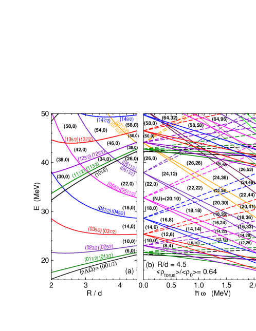
Figure 1: (Color online.) (a) Single-particle states of a toroidal nucleus with $I$=0 as a function of $R/d$, calculated with $\langle\rho_{\rm torus}\rangle/\langle\rho_{0}\rangle$=0.64 and $A$$\sim$40. Each state is labeled by $(n,\Lambda,\Omega)$, with $n$=$n_{z}$+$n_{\rho}$ and degenerate $\Omega_{z}$. (b) Single-particle Routhians of a toroidal nucleus with $R/d$=4.5, as a function of a cranking frequency $\hbar\omega$. Routhians of positive- and negative-$\Omega_{z}$ states are given by the solid and dashed lines, respectively. The listed pair numbers $(N,I)$ refer to the occupation number $N$ and the total angular momentum $I$=$I_{z}$ aligned along the symmetry $z$-axis. Figure taken from Ref. [1].

We consider next the single-particle state diagram for a toroidal nucleus of an aspect ratio $R/d$ under a non-collective rotation with an aligned angular momentum, $I$=$I_{z}$. We use a Lagrange multiplier $\omega$ to describe the constraint $I_{z}$=$\langle\hat{J}_{z}\rangle$=$\sum_{i=1}^{N}\Omega_{zi}$. The constrained single-particle Hamiltonian becomes the Routhian $\hat{h}^{\prime}={\hat{h}}-\omega\hat{J}_{zi}$, and the aligned angular momentum $I$ is a step-wise function of the Lagrange multiplier $\omega$ [13], with each $I$ spanning a small region of $\hbar\omega$. The single-particle Routhian under the constraint of the non-collective aligned angular momentum $I$ is

$$E(n\Lambda\Omega\Omega_{z})\sim\hbar\omega_{0}(n+1)+\frac{\hbar^{2}\Lambda^{2}}{2mR^{2}}-\hbar\omega\Omega_{z}.$$ (2)

Fig. 1(b) gives the single-particle Routhians as a function of the constraining Lagrange multiplier $\hbar\omega$, for a toroidal nucleus with $R/d$=4.5, approximately the aspect ratio for many toroidal nuclei with 28$\leq$$A$$\leq$52. We can use Fig. 1(b) to determine $I$=$I_{z}$ as a function of $N$ and $\hbar\omega$. Specifically, for a given $N$ and $\hbar\omega$, the aligned $I_{z}$-component of the total angular momentum $I$ from the $N$ nucleons can be obtained by summing $\Omega_{zi}$ over all states below the Fermi energy. The energy scales of the $\hbar\omega$ and $E$ axes in Fig. 1(b) depend on $N$, $R/d$, $\langle\rho_{\rm torus}\rangle/\langle\rho_{0}\rangle$ which vary individually at different isomeric toroidal energy minima, but the structure of the $(N,I_{z})$ shells and their relative positions in Fig. 1(b) remain approximately the same in this $A$$\sim$40 mass region. We can use Figs. 1(a) and 1(b) as a qualitative guide to explore the landscape of the energy surface for different $(N,I_{z})$ configurations, by employing a reliable microscopic model. For a proton/neutron number $N$ such that ($N\bmod{4}$)= 0 or 2, Table 1 gives the simple rules to calculate an aligned angular momentum, $I$=$I_{z}$, in terms of particle-hole excitations between the states with $n$=0, relative to the $I$=0 configuration.

Table 1: The quantized values of aligned angular momentum $I$=$I_{z}$ for different particle-hole excitations between the states with quantum number $n$=0 in the N nucleon system. The parameter $\Lambda_{max}=[N-(N\bmod{4})]/4$ is the maximum value of the $z$-component of the orbital angular momentum in the ground state.

Excitation	$N$=$4\Lambda_{max}$	$N$=$4\Lambda_{max}+2$
1p-1h	$I=2\Lambda_{max}$	$I=2\Lambda_{max}+2$
2p-2h	$I=4\Lambda_{max}+1$	$I=4\Lambda_{max}+2$
3p-3h	$I=6\Lambda_{max}$	$I=6\Lambda_{max}+4$
4p-4h	$I=8\Lambda_{max}+1$	$I=8\Lambda_{max}+4$
5p-5h	$I=10\Lambda_{max}$	$I=10\Lambda_{max}+6$

3 Toroidal isomers in Skyrme energy density functional approach

Our objective in the present study is to locate local toroidal figures of equilibrium, if any, in the multi-dimensional search space of $(A$=$N$+$Z$,$Q_{20},I)$ with $N$$\neq$$Z$. To do this we used the Skyrme energy density functional approach where the constraint HFB or cranked HF equations are solved using the symmetry-unrestricted code HFODD [14] and an augmented Lagrangian method [15]. In the particle-hole channel the Skyrme SkM* force [16] was applied and a density-dependent mixed pairing [17, 18] interaction in the particle-particle channel was used in HFB variant. The code HFODD uses the basis expansion method in a three-dimensional Cartesian deformed HO basis. In the present study, we used the basis which consists of 1140 lowest states of deformed HO, having not more than $N_{0}$=26 quanta in the Cartesian directions.

3.1 Toroidal configurations with no rotation

The general occurrence of shell gaps in the single-particle diagrams in Figs. 1(a) and (b) implies that there are many nuclei with different $N$ and $Z$ that will acquire large shell effects, and these shell effects provide some degrees of stability for the nucleus. As a consequence, we expect from Fig. 1(a) that if a nucleus is constrained to possess a large-magnitude negative quadrupole moment and the nucleon numbers $N$ and $Z$ reside on the shell gaps of Fig. 1(a), the density of the nucleus will likely be toroidal in character.

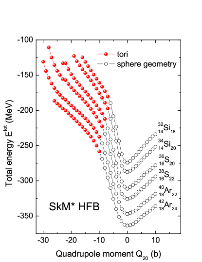
Figure 2: (Colour online.) The total HFB energies of ${}_{14}^{32}$Si, ${}_{14}^{34}$Si, ${}_{16}^{36}$S, ${}_{16}^{38}$S, ${}_{18}^{40}$Ar, ${}_{18}^{42}$Ar, as a function of the quadrupole moment $Q_{20}$ for the case of $I$=0. Toroidal and spherical configurations are indicated by full and open circles, respectively.

Such an expectation is indeed confirmed for the case of $I$=0. The Skyrme-HFB calculations for $N$=$Z$ in Fig. 2 of our earlier work in [1], and for many $N$$\neq$$Z$ nuclei in the present work in Fig. 2, reveal that as the quadrupole moment constraint, $Q_{20}$, decreases to become more negative, the density configurations with sphere-like geometry (open circles) turn into those of an axially-symmetric torus (full circles). Axially-symmetric toroidal density distributions are found in ${}_{14}^{32}$Si, ${}_{14}^{34}$Si, ${}_{16}^{36}$S, ${}_{16}^{38}$S, ${}_{18}^{40}$Ar, and ${}_{18}^{42}$Ar. The presence of the large number of toroidal configurations when there is a large-magnitude negative quadrupole moment constraint suggests that the occurrence of these toroidal configurations are quite common for light nuclei in this mass region, as predicted by Fig. 1(a). As the search is not yet exhaustive, nuclei with toroidal configurations in addition to those in Fig. 2 are possible. Furthermore, because of the approximate symmetry of $N$ and $Z$, toroidal configurations are also expected for the mirror nucleus ${}_{Z}^{A}$$N$, if the ${}_{N}^{A}$$Z$ is found to be in a toroidal configuration.

An examination of the energies of axially-symmetric toroidal configurations as a function of $Q_{20}$ in Fig. 2 reveals however that they lie on a slope. This indicates that even though the shell effects cause the density to become toroidal when there is a quadrupole constraint, the magnitudes of the shell corrections are not sufficient to stabilize the tori against the bulk tendency to return to sphere-like geometry.

3.2 Toroidal configurations with non-collective $I$=$I_{z}$ rotations

From our earlier work on the liquid-drop model of a rotating toroidal nucleus, we expect that an angular momentum about the symmetry axis will have a stabilizing effect on the toroidal nucleus and the nucleus may be stabilized against contraction of the torus, when the angular momentum exceeds a threshold value [5]. We would like to study whether the toroidal nucleus may indeed be stabilized under a non-collective rotation about the symmetry axis in the mean-field theory. Therefore, we take these toroidal configurations obtained for $I$=0 as the initial configurations and set them in a non-collective rotation in $Q_{20}$-constrained cranked Skyrme-HF calculations.

In the case of the non-collective rotation about the symmetry axis, the particle-hole excitations weaken the pairing interaction which can be approximately neglected for large $I$=$I_{z}$ in the cranking approach (see e.g. [19] subsection 3.4). The search for the final toroidal high-spin isomeric state of a light nucleus is facilitated by a good starting point at $I$=0, but there is a great deal of flexibility in choosing this starting point (for example, by choosing alternatively a chain of alpha particles and omitting the pairing interaction [10, 11, 12]). The quantitative measure of the pairing gap for the starting toroidal solution do not affect sensitively the final toroidal equilibrium (high-spin) solution we have obtained.

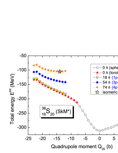
Figure 3: (Color online.) The total energy $E^{\rm tot}$ of toroidal high-spin states of ${}_{16}^{36}$S as a function of $Q_{20}$ for different values of the angular momentum $I$=$I_{z}$. The $n$p-$n$h configurations relative to the $I$=0 configuration are also indicated. The location of isomeric toroidal energy minimum for $I$=74$\hbar$ is indicated by the star symbol.

From the quantum mechanical point of view, the non-collective rotation around the symmetry axis of an axially-symmetric nucleus corresponds simply to $n$-particle $n$-hole ($n$p-$n$h) excitations [9, 20]. For this axially-symmetric toroidal even-even nucleus the occupation of all levels below the Fermi energy leads naturally to the state with $I$=0. The ($n$p-$n$h) excitations relative to this $I$=0 toroidal configuration will lead to high-spin toroidal isomeric states with the total spin given by

$$I=I_{z}=\sum_{i}(\Omega_{zi}^{part}-\Omega_{zi}^{hole}).$$ (3)

For any given $N$ or $Z$ value and $Q_{20}$ deformation constraint we need to estimate the Lagrangian multiplier $\hbar\omega$ that self-consistently leads to the $I$=$I_{z}$ state in the cranked HF calculation. To do this we can use Fig. 1(b) as a qualitative guide to locate the ($N,I$) or ($Z,I$) ‘shells’. Knowing the position of the shell as a function of $\hbar\omega$, we can appropriately increase the value of $\hbar\omega$ in the cranked HF model, to go to the shell in the ’right’ (with larger spin) or decrease $\hbar\omega$ to go to the shell in the ’left’ (with smaller spin). In this way, we can reach all quantized angular momentum $I$ for a specific mass number $A$ as revealed qualitatively by Fig. 1(b). In this connection, it is easy to see that the shell effects of greater stability can be achieved if the shells for e.g. ($N,I_{n}$) and ($Z,I_{p}$) occur at the same value of $\hbar\omega$, leading to the ($A,I=I_{n}+I_{p}$) high-spin configuration at some $Q_{20}$ deformation constraint.

It should be stressed that Fig. 1(b) allows us to estimate the Lagrangian multiplier $\hbar\omega$ only qualitatively and the ’average’ (for $A$$\sim$40 and $R/d$=4.5) values of $\hbar\omega$ in Fig. 1(b) for the specific shells ($N$ or $Z,I$) differ from the values presented in Table 2 for the high-spin toroidal isomers with 28$\leq$$A$$\leq$52.

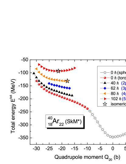
Figure 4: (Color online.) The total energy $E^{\rm tot}$ of toroidal high-spin states of ${}_{18}^{40}$Ar as a function of $Q_{20}$ for different values of the angular momentum $I$=$I_{z}$. The $n$p-$n$h configurations relative to the $I$=0 configuration are also indicated. The locations of isomeric toroidal energy minima for $I$=80$\hbar$ and $I$=102$\hbar$ are indicated by the star symbols.

To find the high-spin toroidal isomer configurations for a given mass number $A$, we use the plots of total energy $E^{\rm tot}$ of the nucleus with the mass number $A$ as a function of the $Q_{20}$, calculated in the cranked constrained SkM*-HF model for all quantum mechanically allowed values of the angular momentum $I$=$I_{z}$. At each point ($Q_{20},I$), where the total energy plot reveals the local energy minimum the quadrupole constraint is removed and free-convergence is tested to ensure that the toroidal nucleus is indeed a figure of equilibrium (a high-spin isomeric state). Figs. 3 and 4 show the results of this method in the case of ${}_{16}^{36}$S and ${}_{18}^{40}$Ar, respectively. We find toroidal high-spin isomers for ${}_{16}^{36}$S($I$=74$\hbar$) and ${}_{18}^{40}$Ar($I$=82, 102$\hbar$).

The toroidal high-spin isomer ${}_{16}^{36}$S($I$=74$\hbar$) arises from the shells at $(Z,I)$=(16,33) and $(N,I)$=(20,41) which are located on the same $\hbar\omega$$\sim$1.8 MeV in Fig. 1(b), corresponding to a 4p-4h excitation of both neutrons and protons (relative to the $I$=0 configuration). Similarly, the toroidal high-spin isomer ${}_{18}^{40}$Ar($I$=80$\hbar$) arises from the shells at $(Z,I)$=(18,36) and $(N,I)$=(22,44) located at $\hbar\omega$$\sim$1.8 MeV in Fig. 1(b), corresponding to a 4p-4h excitation of both neutrons and protons. On the other hand, the ${}_{18}^{40}$Ar($I$=102$\hbar$) toroidal high-spin isomer arises from the shells at $(Z,I)$=(18,46) and $(N,I)$=(22,56) located at $\hbar\omega$$\sim$2.3 MeV in Fig. 1(b), corresponding to a 5p-5h excitation of both neutrons and protons.

3.3 Stability of the toroidal high-spin isomers against nucleon emission

In Figs. 5 and 6, the neutron- and proton-quasiparticle energies obtained in the SkM*-HF+BCS model for toroidal ⁵²Fe with $I$=0 (no rotation) are presented as a function of the quadrupole moment $Q_{20}$. Each of these states is labeled by asymptotic quantum numbers $[Nn_{z}\Lambda]\Omega$. One can see that all states lying below the Fermi level have the quantum numbers $n_{z}=0$ and $\Lambda=0,1,2,\ldots,6$. To illustrate $n$p-$n$h excitations observed in toroidal ⁵²Fe we used solid circular (red) points to mark the high-$\Lambda$ particle states excited from lower-$\Lambda$ hole states marked by open circular points. Each of the $n$p-$n$h excitation configurations is shown at the quadrupole deformation of the toroidal high-spin isomer of ⁵²Fe (see Table 2). It should be mentioned that all occupied excited (particle) states possess the same quantum number $n_{z}=0$ as the hole states, and have ($\Lambda,\Omega$)=(7,15/2), (7,13/2), (8,17/2), (8,15/2), (9,19/2). While the neutron quasiparticle energies of occupied excited states are all negative (Fig. 5), the proton quasiparticle energies of the occupied high-$\Lambda>$7 states are positive (Fig. 6), raising questions whether toroidal high-spin isomers obtained by occupying these high-$\Lambda$ proton states are stable against nucleon emission.

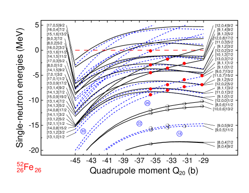
Figure 5: (Color online.) The neutron-quasiparticle energies as a function of the quadrupole moment $Q_{20}$ obtained in the SkM*-HF+BCS model for toroidal ⁵²Fe with $I$=0. They are labeled by $[Nn_{z}\Lambda]\Omega$, with even parity levels as solid lines, and odd parity levels as dashed lines. Starting from the $I$=0 configuration, the 2p-2h, 3p-3h, 4p-4h, and 5p-5h excitations shown in the plot (with holes as open circles and particles in solid circular points) lead to non-collective rotations with a total $I_{z}$=26, 40, 52, and 66$\hbar$, respectively. The horizontal (red) dashed line represents energy $E=0$.

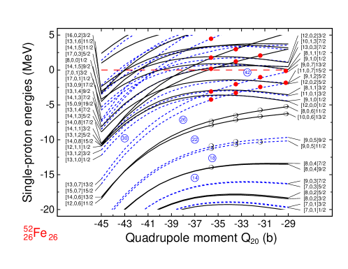
Figure 6: (Color online.) The same as in Fig. 5, but for the proton-quasiparticle energies.

To address this issue, we would like to focus on 5p-5h excitation at $Q_{20}=-35.6$ b. For $N$ or $Z=$26 we can estimate using Table 1 that $\Lambda_{max}=6$ and $I=10\Lambda_{max}+6=66\hbar$ for neutrons and protons, so the total angular momentum along the symmetry axis is $I$=132$\hbar$ in this case. Fig. 7 displays the modulus squared of the neutron (panel (a)) and proton (panel (b)) wave functions of ⁵²Fe with $n_{z}$=0 and $\Lambda$=7,8,9, calculated along $x$-direction in the SkM*-HF+BCS model with constraint $Q_{20}=$$-$36 b. In the same plot we display also the neutron/proton density distributions $\rho_{n/p}$ presented as hatched areas. The same wave functions as in Fig. 7 and the neutron/proton density distributions calculated in the cranked SkM*-HF model in the intrinsic frame ($x^{\prime},y^{\prime},z^{\prime}$) for the toroidal high-spin isomer ⁵²Fe($I$=132$\hbar$) are shown in Fig. 8.

We find that these $n_{z}$=0 and $\Lambda$=7,8,9 wave functions for both $I$=0 (Fig. 7) and $I$=132$\hbar$ (Fig. 8) do not exhibit the unbound characteristics of leakage and oscillation beyond the single-particle potential. They are well localized in the toroidal region of the attractive mean-field potential and they have Gaussian shapes very similar to those wave functions of lower-lying bound single-particle states. In contrast, the wave functions of the [10,1,1]1/2 state in Figs. 7 and 8 that are not used for the construction of the toroidal isomer - extend outside the single-particle potential. We also tested our model for a well-known unbound $3s_{1/2}$ state in the ground state of ³²Fe (at $Q_{20}=1.6$ b) and we found that the $3s_{1/2}$ single-particle energy is positive and the spatial wave function leaks to the region of large $r$ with an oscillating amplitude extending beyond the single-particle potential. This indicates that deformed HO basis used in our study is sufficient to properly describe the scattering (unbound) states and our model allows us to discern different properties of the scattering and bound states.

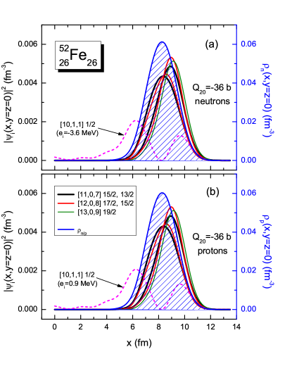
Figure 7: (Color online.) (a) The modulus squared of the neutron wave functions $[N,n_{z}$=0,$\Lambda$=7,8,9$]\Omega$, representing the particle states in the $n$p-$n$h excitations of ⁵²Fe (see Figs. 5 and 6). The state wave functions and the density distributions $\rho_{n}$ (the hatched area) were calculated in the SkM*-HF+BCS model with a constraint on the quadrupole moment, $Q_{20}$=-36 b, which is close to the deformation of the toroidal ⁵²Fe(132$\hbar$) isomer. On the same plot is shown, as an example, the modulus squared of the state wave function $[10,1,1]1/2$ which is not used in the construction of the toroidal configurations. Panel (b) the same as in the panel (a), but for the proton wave functions and proton density distribution $\rho_{p}$.

There may be two possible reasons why there are no apparent wave function leakage and oscillations at large $r$ for these $n_{z}$=0 and $\Lambda$=7,8,9 states used for the construction of the toroidal high-spin isomer: (i) the ’confinement’ of these single-particle states with exponentially decaying probability to reach $r\to\infty$ beyond the single-particle potential or (ii) the presence of large centrifugal and additional proton Coulomb barriers, allowing only a small penetration probability for tunneling to $r\to\infty$.

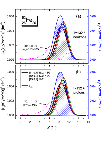
Figure 8: (Color online.) The same as in Fig. 7, but the wave functions and the neutron/proton density distributions were calculated in the cranked SkM*-HF model for the equilibrium configuration of the isomeric toroidal state ⁵²Fe(132$\hbar$).

To study further which of the above two possibilities pertains to the wave functions of the high-$\Lambda$ states for our toroidal isomers in question, we consider the single-particle equation

$$(-\frac{\hbar^{2}}{2m}\triangle+V(r,z))\Psi_{E}(\bm{r})=E\Psi_{E}(\bm{r}),$$ (4)

where $V(r,z)=U(r)+W(z)$ is an axially symmetric non-central potential with a minimum at $V(R,0)$. We assume that $\lim_{r\to\infty}U(r)=0$ and $\lim_{|z|\to\infty}W(z)=0$. If the potential is analytic near its minimum, we can make a Taylor expansion about the point ($r,z$)=($R,0$)

$$V(r,z) = U(R)+W(0)+\left.\frac{dU}{dr}\right|_{r=R}(r-R)+\left.\frac{dW}{dz}\right|_{z=0}z$$ (5)

$$+\left.\frac{1}{2!}\frac{1}{r}\frac{d}{dr}\left(r\frac{dU}{dr}\right)\right|_{r=R}(r-R)^{2}+\left.\frac{1}{2!}\frac{d^{2}W}{dz^{2}}\right|_{z=0}z^{2}+\cdots.$$

At the minimum the first-order derivatives vanish and we can set constants to zero, $U(R)=W(0)=0$. If we now shift a radial coordinate $r$ to $r+R$ Eq. (5) reads

$$V(r,z) = \left.\frac{1}{2!}\frac{d^{2}U}{dr^{2}}\right|_{r=R}r^{2}+\left.\frac{1}{2!}\frac{d^{2}W}{dz^{2}}\right|_{z=0}z^{2}+\cdots$$ (6)

$$\approx U(r)+\frac{1}{2}m\omega^{2}_{z}z^{2},$$ (7)

where

$$\omega^{2}_{z}=\left.\frac{1}{m}\frac{d^{2}W}{dz^{2}}\right|_{z=0}.$$ (8)

The high-spin toroidal isomers under consideration have been constructed with single-particle states whose wave functions in the $z$-direction reside in the lowest state, with a zero number of nodes, $n_{z}$=0. Using the approximation (7), we can express energy associated with a $z$-degree of freedom of the $n_{z}$=0 bound states by the zero-point energy $E_{0z}=\frac{1}{2}\hbar\omega_{z}$.

Writing $\Psi=P(r)\frac{1}{\sqrt{2\pi}}e^{i\Lambda\varphi}Z_{0}(z)$, where $Z_{0}(z)=\left(\frac{a}{\pi}\right)^{1/4}e^{-az^{2}/2}$ with $a=m\omega_{z}/\hbar$, and using the method of separation of variables we receive the radial equation

$$\left[\frac{d^{2}}{dr^{2}}+\frac{1}{r}\frac{d}{dr}+\frac{2m}{\hbar^{2}}(E_{\bot}(i)-U(r))-\frac{\Lambda^{2}}{r^{2}}\right]P_{i}(r)=0,$$ (9)

where $\Lambda$ can have any integer value and the energy of the $r$-direction (transverse) motion, $E_{\bot}(i)$, is equal to the difference between a total singe-particle energy, $E(i)$, and the zero-point energy for the motion in the $z$-direction:

$$E_{\bot}(i)=E(i)-\frac{1}{2}\hbar\omega_{z}.$$ (10)

We provide the solution to Eq. (9) in Appendix A, where we use a finite square potential well to describe the radial potential $U(r)$.

The bound states of the nucleon occur when the energy available for motion in the $r$-direction is $E_{\bot}(i)$$<$0. We have carried out an analysis to check the signs of the $E_{\bot}(i)$ values for those occupied single-particle states in the toroidal ⁵²Fe($I$=132$\hbar$) isomer for which the signs of total single-particle energies $E(i)$ are positive. The zero-point energy $\frac{1}{2}\hbar\omega_{z}$ for the single-particle states can be extracted from the plots of their modulus squared wave functions $|\psi_{i}(r=R,z)|^{2}$ plotted in the $z$-direction. For example, the zero point energy for the topmost occupied state, [N,0,9]19/2, in the toroidal high-spin isomer ⁵²Fe($I$=132$\hbar$) is equal 8.0 MeV for neutrons and protons. From these $E_{0z}=\frac{1}{2}\hbar\omega_{z}$ and Eq. (10), the single-particle energies for radial motion $E_{\bot}(i)$ can be calculated. The self-consistent calculations in the toroidal isomer ⁵²Fe($I$=132$\hbar$) reveal that $E_{\bot}(i)$ for the $n_{z}$=0 and $\Lambda$=7,8,9 states are negative, leading to exponentially decaying single-particle radial wave functions, $P_{i}(r)$, for large values of $r$. This indicates that wave functions of these occupied single-particle states in toroidal ⁵²Fe($I$=132$\hbar$) isomer are not only localized but also square integrable. However, it should be stressed that any $n$p-$n$h particle state with $E(i)>\frac{1}{2}\hbar\omega_{z}$ will not hold a bound state. Thus, one expects an $I_{z}$-window for which bound states are possible.

It is worth noting that what we have observed are the states with the positive total energy $E(i)$ whose wave functions are localized in the $z$- and $r$-directions and are square integrable. These states seem analogous to the bound states in the continuum (BIC) first suggested by von Neumann and Wigner in 1929 [21] (see also [22]) and recently examined by many workers in various quantum and optical systems (see e.g. [23] and references cited therein).

4 Properties of $N$$\neq$$Z$ toroidal high-spin isomers

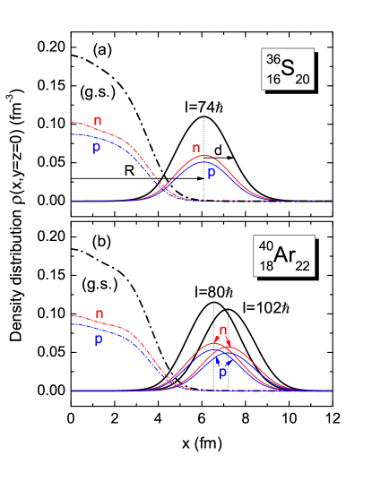
Figure 9: (Color online.) (a) The total density distribution of the isomeric toroidal state of ${}_{16}^{36}$S with $I$=74$\hbar$ as a cut in the radial direction $x$. We show the major radius $R$ and the minor radius $d$ of toroidal density distribution. The dash-dot curve shows the total density distribution in the ground state (g.s.) of ${}_{16}^{36}$S. Lines indicated by n/p represent the neutron/proton density distributions, respectively. (b) Total density distributions of the isomeric toroidal states of ${}_{18}^{40}$Ar with $I$= 80 and 102$\hbar$ as a cut in the radial direction $x$, all symbols are the same as in (a).

After we have located the toroidal high-spin isomers at their energy minima, we can evaluate their properties. We plot in Fig. 9(a) and (b) the density distributions of the toroidal isomers ${}_{16}^{36}$S($I$=74$\hbar$) (presented in Fig. 3) and ${}_{18}^{40}$Ar($I$=80, 102$\hbar$) (Fig. 4), as a cut in the radial direction $x$. For comparison, we also show the total density distribution of ${}_{16}^{36}$S and ${}_{18}^{40}$Ar in their ground state (g.s.) (dash-dot curve) which have a maximum $\rho_{max}$ value distinctly larger than the $\rho_{max}$ of the toroidal high-spin isomers. This is a general property similar to those of other $N$=$Z$ toroidal high-spin isomers [1]. In the case of ${}_{18}^{40}$Ar nucleus when the aligned angular momentum $I$ increases from $I$=80$\hbar$ to $I$=102$\hbar$, the maximum toroidal density $\rho_{max}$ decreases from 0.116 to 0.107 fm^-3 and the major radius $R$ increases from 6.56 to 7.21 fm. Only the minor radius $d$, defined as a half width at half maximum (HWHM) of the toroidal distribution, stays constant at $d\approx$1.37 fm. In addition to the total density distributions we compare in Fig. 5 the neutron (n) and proton (p) density distributions in the toroidal isomeric states as well as in g.s. of ${}_{16}^{36}$S and ${}_{18}^{40}$Ar.

Table 2: Properties of the high-spin toroidal isomers at their local energy minima in 28$\leq$$A$$\leq$52. For nuclei with N=Z all values are taken from Ref. [1]. The angular momentum $I$ is a step-wise function for a range of $\hbar\omega$, for which we give one of the points in the range.

	$I/\hbar$	$Q_{20}$	$\hbar\omega$	$E^{*}$	$R$	$d$	$R/d$	$\rho_{\rm max}$
		(b)	(MeV)	(MeV)	(fm)	(fm)		(fm-3)
${}_{14}^{28}$Si	44	-5.86	$2.8$	143.18	4.33	1.45	2.99	0.119
${}_{16}^{32}$S	48	-8.22	$1.9$	153.87	4.87	1.42	3.43	0.122
	66	-10.51	$2.2$	193.35	5.57	1.40	3.98	0.108
${}_{16}^{36}$S	74	-13.95	$1.85$	205.87	6.08	1.39	4.37	0.112
${}_{18}^{36}$Ar	56	-11.31	$1.7$	168.03	5.44	1.40	3.88	0.125
	72	-13.73	$1.85$	198.63	6.04	1.39	4.34	0.113
	92	-16.78	$2.0$	238.56	6.73	1.37	4.91	0.103
${}_{18}^{40}$Ar	80	-17.83	$1.65$	215.49	6.56	1.38	4.75	0.116
	102	-21.37	$1.85$	253.42	7.21	1.37	5.26	0.107
${}_{20}^{40}$Ca	60	-14.96	$1.5$	178.36	5.97	1.40	4.26	0.126
	82	-17.61	$1.9$	214.23	6.51	1.39	4.68	0.117
${}_{22}^{44}$Ti	68	-19.57	$1.2$	195.46	6.55	1.39	4.71	0.128
	88	-22.27	$1.4$	223.09	7.01	1.38	5.08	0.120
	112	-25.76	$1.6$	260.24	7.56	1.37	5.52	0.113
${}_{24}^{48}$Cr	72	-25.08	$1.2$	207.12	7.12	1.38	5.16	0.128
	98	-28.00	$1.4$	239.26	7.54	1.37	5.50	0.122
	120	-30.55	$1.43$	271.02	7.90	1.36	5.81	0.118
${}_{26}^{52}$Fe	52	-29.24	$0.8$	202.86	7.39	1.38	5.35	0.134
	80	-31.43	$0.95$	227.54	7.68	1.38	5.56	0.130
	104	-33.54	$1.3$	252.65	7.94	1.37	5.79	0.126
	132	-35.62	$1.5$	288.91	8.20	1.36	6.03	0.123

With the additional information on the $N$$\neq$$Z$ isomers, we collect the properties of all known 21 toroidal high-spin isomers in Table 2 and Fig. 10. In Table 2, we list the quantized angular momentum $I$ of the toroidal isomers, its corresponding quadrupole moment $Q_{20}$, the excitation energy $E^{*}$ of the isomer relative to the ground state configuration, the major radius $R$ of the toroid, the minor radius $d$ of the toroid, and the maximum density of the isomer $\rho_{\max}$. The angular momentum $I$ is a step-wise function of the cranking frequency $\hbar\omega$ [13], and there is a range of the cranking frequency (energy) $\hbar\omega$ at which the toroidal high-spin isomer is located. We list the value $\hbar\omega$ of a point within the range in Table 2. These quantities provide a wealth of information about the high-spin toroidal isomers from which properties on the nuclear fluid in the exotic toroidal shape may be extracted.

It is useful to classify the isomers according to their $n$p-$n$h attributes relative to their corresponding $I$=0 configurations. One finds that the all $n$p-$n$h families follow regular well-behaved pattern as shown in Fig. 10, where we plot the total energy of the toroidal isomers as a function of the toroidal aspect ratio $R/d$. The corresponding angular momentum associated with each isomer is also listed. It is important to notice that $N$$\neq$$Z$ nuclei fit very well to the same pattern as $N$=$Z$ nuclei, indicating a smooth behavior for all even-even toroidal high-spin isomers.

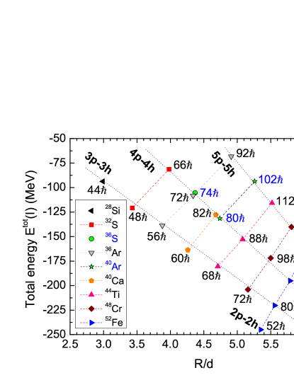
Figure 10: (Color online.) The total energies of the isomeric toroidal states of ${}_{14}^{28}$Si, ${}_{16}^{32}$S, ${}_{16}^{36}$S, ${}_{18}^{36}$Ar, ${}_{18}^{40}$Ar, ${}_{20}^{40}$Ca, ${}_{22}^{44}$Ti, ${}_{24}^{48}$Cr, and ${}_{26}^{52}$Fe and their associated $I$ values (Table 1), as a function of $R/d$. The $n$p-$n$h configurations relative to the $I$=0 configuration are also indicated.

Table 2 further reveals that in each $n$p-$n$h family, the angular momentum and the aspect ratio $R/d$ increase approximately linearly with the mass number while the minor radius $d$ remains essentially unchanged. One can use Table 2 and Fig. 10 to extrapolate the properties of toroidal high-spin isomers in the higher mass region.

5 Conclusions and discussion

Nuclei under non-collective rotation with a large angular momentum about the symmetry axis above a threshold can assume a toroidal shape. We have developed a systematic method of cranked SHF approach by which the high-spin toroidal isomer states can be theoretically located. The application of the method to study nuclei in all regions of the periodical table will enhance our knowledge of the multi-faceted nature of the nuclear phenomenon, allow us to explore into the possibility of toroidal isomers as a source of energy, and permit the study of nuclear fluid in extreme geometry and angular momenta.

Our investigation into the region of nuclei with $N$$\neq$$Z$ indicates that just as the $N$=$Z$ nuclei, toroidal high-spin nuclei are also commonly present. In the present work, we have located the toroidal ${}_{16}^{36}$S($I$=74$\hbar$) and ${}_{18}^{40}$Ar($I$=80, 102$\hbar$) isomers. As indicated in Fig. 2, many other nuclei with other neutron and proton numbers also have axial-symmetric toroidal density distributions under a large-magnitude negative quadrupole moment constraint. We expect that when these nuclei are set to undergo non-collective rotation beyond a threshold, toroidal energy minima and additional toroidal high-spin isomers will be present. Furthermore, because of the approximate symmetry of $N$ and $Z$, toroidal configurations are also expected for the mirror nucleus ${}_{Z}^{A}$$N$, if the ${}_{N}^{A}$$Z$ is found to be in a toroidal configuration. The results obtained here and in Ref. [1] provide a wealth of information to allow the extrapolation in future search of other toroidal nuclei. Extrapolation from Table 2 and Fig. 10 would predict possible occurrence of toroidal high-spin isomers in the mass region of $A$$\sim$60.

Returning to the questions we have posed in the beginning, the occurrence of these $N$$\neq$$Z$ toroidal high-spin isomers shows that it is not necessary to be $\alpha$-particle-type nuclei to be a toroidal high-spin isomer. The conditions for the occurrence of the toroidal high-spin isomer consist of (i) the occurrence of favorable shell-model configuration such as those indicated by the single-particle diagram similar to Figs. 1(a) and (b), and (ii) the quantized angular momentum value exceeding a threshold value. There is a third condition on the maximum limit of $I$=$I_{z}$ and its relation to sausage instabilities that has been examined only for a few cases at the present moment and has not yet received sufficient attention to render a definitive conclusion.

Appendix A

In this appendix we provide the solution to the radial equation

$$\left[\frac{d^{2}}{dr^{2}}+\frac{1}{r}\frac{d}{dr}+\frac{2m}{\hbar^{2}}(E_{\bot}(i)-U(r))-\frac{\Lambda^{2}}{r^{2}}\right]P_{i}(r)=0,$$ (11)

where $E_{\bot}(i)=E(i)-\frac{1}{2}\hbar\omega_{z}$, and $\Lambda$ can have any integer value.

To solve radial equation (11) we use a square well approximation for the radial potential $U(r)$:

$$U(r)=\left\{\begin{array}[]{ll}U_{0}(<0)&\textrm{for }R-d\leq r\leq R+d\\ 0&\textrm{for }R-d>r>R+d,\end{array}\right.$$ (12)

where $R$ and $d$ are the major- and minor-radius of torus, respectively. Then, the radial function, for bound states with $-|U_{0}|<E_{\bot}(i)<0$, obeys

$$r^{2}\frac{d^{2}P_{i}}{dr^{2}}+r\frac{dP_{i}}{dr}+\left(k^{2}_{0z}r^{2}-\Lambda^{2}\right)P_{i}=0,$$ (13)

where the radial wavenumber, $k$, is defined by

$$k^{2}_{0z}=\left\{\begin{array}[]{ll}\frac{2m}{\hbar^{2}}(E_{\bot}(i)+|U_{0}|)\equiv\alpha^{2}&\textrm{for }R-d\leq r\leq R+d\\ \frac{2m}{\hbar^{2}}E_{\bot}(i)\equiv-\beta^{2}&\textrm{for }R-d>r>R+d.\end{array}\right.$$ (14)

If we change variable $r$ to $\alpha r$ in the region $R-d\leq r\leq R+d$ the radial function $P_{i}$ satisfies the Bessel’s ODE. Similarly, if we change variable $r$ to $i\beta r$ in $R-d>r>R+d$ the radial function $P_{i}$ satisfies the modified Bessel’s ODE. A general solution for the radial function takes a form

$$P_{i}=\left\{\begin{array}[]{ll}A^{\prime}I_{|\Lambda|}(\beta r)+B^{\prime}K_{|\Lambda|}(\beta r)&\textrm{for }r<R-d\\ AJ_{|\Lambda|}(\alpha r)+BY_{|\Lambda|}(\alpha r)&\textrm{for }R-d\leq r\leq R+d\\ A^{\prime\prime}I_{|\Lambda|}(\beta r)+B^{\prime\prime}K_{|\Lambda|}(\beta r)&\textrm{for }r>R+d,\end{array}\right.$$ (15)

where we use the standard Bessel function of the first kind, $J_{\Lambda}$, and Bessel function of the second kind, $Y_{\Lambda}$, as well as the modified Bessel function of the first kind, $I_{\Lambda}$, and the modified Bessel function of the second kind (the modified Hankel function), $K_{\Lambda}$. Since for integer order $\Lambda$, $J_{\pm\Lambda}$, $Y_{\pm\Lambda}$, $I_{\pm\Lambda}$, and $K_{\pm\Lambda}$ are not linearly independent, we use the absolute value of $\Lambda$ in Eq. (15).

The radial function must be finite everywhere including at the origin, therefore the constant $B^{\prime}$ has to be equal zero, because the modified Bessel function of the second kind, $K_{|\Lambda|}$, is singular at the origin. Also $A^{\prime\prime}=0$, due to divergent behavior of $I_{|\Lambda|}$ at infinity. Finally, the solution of radial equation (13) for an energy in the interval $-|U_{0}|<E_{\bot}(i)<0$ reads

$$P_{i}=\left\{\begin{array}[]{ll}A^{\prime}I_{|\Lambda|}(\beta r)&\textrm{for }r<R-d\\ AJ_{|\Lambda|}(\alpha r)+BY_{|\Lambda|}(\alpha r)&\textrm{for }R-d\leq r\leq R+d\\ B^{\prime\prime}K_{|\Lambda|}(\beta r)&\textrm{for }r>R+d.\end{array}\right.$$ (16)

The equations that permit us to calculate the eigenvalues are the continuity condition of the logarithmic derivative of $P_{i}$ at $r=R-d$ and $r=R+d$:

$$\left.\frac{I^{\prime}_{|\Lambda|}(\beta r)}{I_{|\Lambda|}(\beta r)}\right|_{r=R-d}=\left.\frac{AJ^{\prime}_{|\Lambda|}(\alpha r)+BY^{\prime}_{|\Lambda|}(\alpha r)}{AJ_{|\Lambda|}(\alpha r)+BY_{|\Lambda|}(\alpha r)}\right|_{r=R-d},$$ (17)

$$\left.\frac{K^{\prime}_{|\Lambda|}(\beta r)}{K_{|\Lambda|}(\beta r)}\right|_{r=R+d}=\left.\frac{AJ^{\prime}_{|\Lambda|}(\alpha r)+BY^{\prime}_{|\Lambda|}(\alpha r)}{AJ_{|\Lambda|}(\alpha r)+BY_{|\Lambda|}(\alpha r)}\right|_{r=R+d},$$ (18)

where we shall adopt the notation that the prime is derivative with respect to $r$. Using formulas for derivatives of the Bessel functions and the modified Bessel functions the continuity condition equations take the form

$$\beta\left.\frac{I_{|\Lambda|+1}(\beta r)}{I_{|\Lambda|}(\beta r)}\right|_{r=R-d} = -\alpha\left.\frac{\mathcal{Z}_{|\Lambda|+1}(\alpha r)}{\mathcal{Z}_{|\Lambda|}(\alpha r)}\right|_{r=R-d},$$ (19)

$$\beta\left.\frac{K_{|\Lambda|+1}(\beta r)}{K_{|\Lambda|}(\beta r)}\right|_{r=R+d} = \alpha\left.\frac{\mathcal{Z}_{|\Lambda|+1}(\alpha r)}{\mathcal{Z}_{|\Lambda|}(\alpha r)}\right|_{r=R+d},$$ (20)

where we introduce shorthand notation (a cylinder function $\mathcal{Z}$)

$$\mathcal{Z}_{|\Lambda|}(\alpha r)=AJ_{|\Lambda|}(\alpha r)+BY_{|\Lambda|}(\alpha r).$$ (21)

Eliminating constants $A$ and $B$ from Eqs. (19) and (20) we obtain the eigenvalue equation

$$\alpha^{2}\;I_{|\Lambda|}(\beta(R-d))K_{|\Lambda|}(\beta(R+d))$$ (22)

$$\left[J_{|\Lambda|+1}(\alpha(R+d))Y_{|\Lambda|+1}(\alpha(R-d))-J_{|\Lambda|+1}(\alpha(R-d))Y_{|\Lambda|+1}(\alpha(R+d))\right]$$

$$+ \beta^{2}\;I_{|\Lambda|+1}(\beta(R-d))K_{|\Lambda|+1}(\beta(R+d))$$

$$\left[J_{|\Lambda|}(\alpha(R-d))Y_{|\Lambda|}(\alpha(R+d))-J_{|\Lambda|}(\alpha(R+d))Y_{|\Lambda|}(\alpha(R-d))\right]$$

$$+ \alpha\beta\;I_{|\Lambda|+1}(\beta(R-d))K_{|\Lambda|}(\beta(R+d))$$

$$\left[J_{|\Lambda|+1}(\alpha(R+d))Y_{|\Lambda|}(\alpha(R-d))-J_{|\Lambda|}(\alpha(R-d))Y_{|\Lambda|+1}(\alpha(R+d))\right]$$

$$+ \alpha\beta\;I_{|\Lambda|}(\beta(R-d))K_{|\Lambda|+1}(\beta(R+d))$$

$$\left[J_{|\Lambda|+1}(\alpha(R-d))Y_{|\Lambda|}(\alpha(R+d))-J_{|\Lambda|}(\alpha(R+d))Y_{|\Lambda|+1}(\alpha(R-d))\right]$$

$$= 0,$$

where $\alpha=\sqrt{\frac{2m}{\hbar^{2}}(|U_{0}|-|E_{\bot}(i)|)}$, $\beta=\sqrt{\frac{2m}{\hbar^{2}}|E_{\bot}(i)|}\neq 0$.

There are no solutions to Eq. (22) if $E_{\bot}(i)<-|U_{0}|$. In the energy range $-|U_{0}|<E_{\bot}(i)<0$ there is the discrete spectrum. Since $E_{\bot}(i)=0$ is a continuous spectrum limit, we see that in terms of $E(i)=E_{\bot}(i)+\frac{1}{2}\hbar\omega_{z}$ the continuum limit is equal to the zero point energy of the $z$-direction motion $E(i)=\frac{1}{2}\hbar\omega_{z}$. The continuous spectrum exists for $E>\frac{1}{2}\hbar\omega_{z}$ ($E_{\bot}>0$) and the radial wave function takes the form

$$P=\left\{\begin{array}[]{ll}A^{\prime}J_{|\Lambda|}(\beta r)&\textrm{for }r<R-d\\ AJ_{|\Lambda|}(\alpha r)+BY_{|\Lambda|}(\alpha r)&\textrm{for }R-d\leq r\leq R+d\\ A^{\prime\prime}J_{|\Lambda|}(\beta r)+B^{\prime\prime}Y_{|\Lambda|}(\beta r)&\textrm{for }r>R+d,\end{array}\right.$$ (23)

with $\alpha^{2}=\frac{2m}{\hbar^{2}}(E_{\bot}+|U_{0}|)$ and $\beta^{2}=\frac{2m}{\hbar^{2}}E_{\bot}$.

We would like to point out that similar quantum systems supporting an old idea of a so-called bound state in the continuum (BIC), suggested by von Neumann and Wigner [21],were discussed by Robnik [24] and recently in Ref. [23].

References

References

- [1] Staszczak A and Wong C Y 2014 Phys. Lett. B 738 401
- [2] See a reference to J. A. Wheeler’s toroidal nucleus in Gamow G 1961 Biography of Physics (New York: Harper & Brothers Publishers) pp. 297
- [3] Wong C Y 1973 Ann. of Phys. (N.Y.) 77 279
- [4] Staszczak A and Wong C Y 2008 Acta Phys. Pol. B 40 753, and references cited therein
- [5] Wong C Y 1978 Phys. Rev. C 17 331
- [6] Eggers J 1997 Rev. Mod. Phys. 69 865
- [7] Pairam E and Fernández-Nieves A 2009 Phys. Rev. Lett. 102 234501
- [8] Vautherin D and Brink D M 1972 Phys. Rev. C 5 626; Engel Y M, Brink D M, Goeke K, Krieger S, and Vautherin D 1975 Nucl. Phys. A 249 215
- [9] Bohr A and Mottelson B R 1981 Nucl. Phys. A 354 303c
- [10] Ichikawa T, Maruhn J A, Itagaki N, Matsuyanagi K, Reinhard P-G, and Ohkubo S 2012 Phys. Rev. Lett. 109 232503
- [11] Ichikawa T, Matsuyanagi K, Maruhn J A, and Itagaki N 2014 Phys. Rev. C 89 011305(R)
- [12] Ichikawa T, Matsuyanagi K, Maruhn J A, and Itagaki N 2014 Phys. Rev. C 90 034314
- [13] Ring P and Schuck P 1980 The Nuclear Many-Body Problem (Springer-Verlag, Berlin, Heidelberg, New York) pp. 142
- [14] Schunck N et al. 2012 Comput. Phys. Commun. 183 166
- [15] Staszczak A, Stoitsov M, Baran A, and Nazarewicz W 2010 Eur. J. Phys. A 46 85
- [16] Bartel J, Quentin P, Brack M, Guet C, and Håkansson H B 1982 Nucl. Phys. A 386 79
- [17] Dobaczewski J, Nazarewicz W, and Stoitsov M V 2002 Eur. J. Phys. A 15 21
- [18] Staszczak A, Baran A, Dobaczewski J, and Nazarewicz W 2009 Phys. Rev. C 80 014309
- [19] Afanasjev A V, Fossan D B, Lane G J, and Ragnarsson I 1999 Phys. Rep. 322 1
- [20] de Voigt M J A, Dudek J, and Szymański Z 1983 Rev. Mod. Phys. 55 949
- [21] von Neumann J and Wigner E 1929 Phys. Z. 30 465
- [22] Stillinger F H and Herrick D R 1975 Phys. Rev. A 11 446
- [23] Prodanović N, Milanović V, Ikonić Z, Indjin D, and Harrison P 2013 Phys. Lett. A 337 2177
- [24] Robnik M 1986 J. Phys. A 19 3845