Femtoscopic Signature of Strong Radial Flow
in High-multiplicity $pp$ Collisions

Abstract

Hydrodynamic simulations are used to calculate the identical pion HBT radii, as a function of the pair momentum $k_{\rm T}$. This dependence is sensitive to the magnitude of the collective radial flow in the transverse plane, and thus comparison to ALICE data enables us to derive its magnitude. By using hydro solutions with variable initial parameters we conclude that in this case fireball explosions start with a very small initial size, well below 1 ${\rm fm}$.

I Introduction

The so-called Hanbury-Brown-Twiss (HBT) interferometry method originally came from radio astronomy Brown and Twiss (1956) as intensity interferometry. The influence of Bose symmetrization of the wave function of the observed mesons in particle physics was first emphasized by Goldhaber et al. Goldhaber et al. (1960) and applied to proton-antiproton annihilation. Its use for the determination of the size and duration of the particle production processes had been proposed by Kopylov and Podgoretsky Kopylov and Podgoretsky (1974) and one of us Shuryak (1973). Heavy-ion collisions, with their large multiplicities, turned the “femtoscopy” technique into a large industry. Early applications for RHIC heavy-ion collisions were in certain tension with the hydrodynamical models, but this issue was later resolved; see, e.g., Pratt (2009). The development of the HBT method had made it possible to detect the magnitude and even deformations of the flow.

Makhlin and Sinyukov Makhlin and Sinyukov (1988) made the important observation that HBT radii are sensitive to collective flows of matter. The radii decrease with the increase of the total transverse momentum $\bm{k}_{\rm T}=(\bm{p}_{\rm 1T}+\bm{p}_{\rm 2T})/2$ of the pair. A sketch shown in Fig.1 provides a qualitative explanation of this effect: the larger is $k_{\rm T}$, the brighter becomes a small (shaded) part of the fireball, the radial flow of which is maximal and its direction coincides with the direction of $\bm{k}_{\rm T}$. This follows from maximization of the Doppler-blue shifted thermal spectrum $\sim\exp\left(-p^{\mu}u_{\mu}/T_{\rm f}\right)$. In this paper we will rely on this effect, as well as on ALICE HBT data, to deduce the magnitude of the flow in high multiplicity $pp$ collisions.

(Although we will not use those, let us also mention that the HBT method can also be used not only for determination of the radial flow, but for elliptic flow as well; see, e.g., early STAR measurements Adams et al. (2004). Another development in the HBT field was a shift from two-particle to three-particle correlations Adams et al. (2003), Abelev et al. (2014) available due to very high multiplicity of events as well as high luminosities of RHIC and LHC colliders.)

With the advent of the LHC it became possible to trigger on high-multiplicity events, both in $pp$ and $pPb$ collisions: the resulting sample revealed angular anisotropies $v_{2},v_{3}$ similar to anisotropic flows in heavy-ion ($AA$) collisions. At the moment the issue of whether those can or cannot be described hydrodynamically is under debate. So far the discussion of the strength of the radial flow has been based on the spectra of identified particles; see Shuryak and Zahed (2013); Ghosh et al. (2014). In this paper we look at the radial flow from a different angle, using the measured HBT radii Aggarwal et al. (2011).

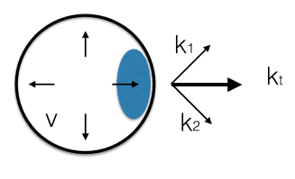
Figure 1: (Color online) Sketch of how the radial flow (arrows directed radially from the fireball center) influences the HBT radii. At small $k_{\rm T}$ the whole fireball (the circle) is visible, but at larger $k_{\rm T}$ one sees only the part comoving in the same direction, shown by the shaded ellipse.

The HBT radii for $pp$ collisions at the LHC have been measured by the ALICE Collaboration Aggarwal et al. (2011), as a function of multiplicity. Their magnitude has been compared to those coming from hydro modeling in Refs. Shapoval et al. (2013); Sinyukov and Shapoval (2013). Our analysis of the HBT radii focus on the strength of the radial flow. We illustrate how the radii, and especially the ratio $R_{o}/R_{s}$, are indicative of the flow magnitude.

While at minimally biased collisions and small multiplicities the observed HBT radii are basically independent of the pair transverse momentum $k_{\rm T}$, for high multiplicity the observed radii decrease with $k_{\rm T}$. So, the effect we are after appears only at the highest multiplicities – the same ones which display hydro-like angular correlations and modifications of the particle spectra. The strongest decrease, as expected, is seen for the so-called $R_{o}$ radius, for which this reduction in the interval $k_{\rm T}=0.1-0.7\,{\rm GeV}$ reaches about factor 4 in magnitude.

The $k_{\rm T}$ dependence of the HBT radii tells us about the strength of the flow. The reason these data are quite important is the following: the HBT radii at small $k_{\rm T}$ tell us the $final$ size of the fireball, at the freezeout. The radii at large $k_{\rm T}$, combined with hydro calculations to be described below, can shed light on the $initial$ size of the fireball, which we consider to be the main result of this work.

We do not speculate below on how such initial conditions can be created: this should be determined by models of the initial state. Our goal is only to derive phenomenologically its parameters. Their importance stems from the fact that high-multiplicity $pp$ collisions create the most extreme conditions of matter density reached so far.

II Method of analysis

II.1 Hydrodynamic evolution

For heavy-ion collisions one has good command of the matter distribution in nuclei, and thus can model the shape of the initial state rather accurately. However in the case of high-multiplicity $pp$ collisions – which are certain fluctuations with small probability – there is still no quantitative theory, and thus the shape remains unknown.

A certain shape is preferable, not on physical but technical grounds. An analytic solution known as Gubser flow Gubser (2010) is restricted to a shape appearing in a stereographic projection from a sphere to the transverse plane. Using the same shape had allowed us to compare our numerical solution to the corresponding analytic expression, providing control of the code numerical accuracy.

In the Gubser solutions, the energy density and velocity take the form

$$\epsilon(\tau,r)=\frac{\epsilon_{0}(2q)^{8/3}}{\tau^{4/3}[1+2q^{2}(\tau^{2}+r^{2})+q^{4}(\tau^{2}-r^{2})^{2}]^{4/3}},$$ (1)

$$v_{\perp}(\tau,r)=\frac{2q^{2}\tau r}{1+q^{2}\tau^{2}+q^{2}r^{2}}.$$ (2)

The space-time characteristics of the system are parametrized by two variables,

$$\left(\,q\ [{\rm fm}^{-1}],\,\,\epsilon_{0}\,\right).$$ (3)

(The parameter $q$ is widely used below, not to be confused with the momentum transfer.) The dimensionless energy density parameter $\epsilon_{0}$ is related with the entropy per unit rapidity as

$$\epsilon_{0}=f_{\ast}^{-1/3}\left(\frac{3}{16\pi}\frac{dS}{d\eta}\right)^{4/3},$$ (4)

where $f_{\ast}=11$ is the number of effective degrees of freedom in QGP Gubser (2010). The entropy per unit rapidity is inferred from the measured charged particle multiplicity,

$$\frac{dS}{d\eta}\simeq 7.5\frac{dN_{\rm ch}}{d\eta}.$$ (5)

Thus, the values of $\epsilon_{0}$ can be fixed by charged particle multiplicity.

On the other hand, the parameter $q$ quantifies the size of the system. Figure 2 shows the temperature profiles at $\tau=0.6\ {\rm fm}$ as a function of $r$ for $q=1.7\ {\rm fm}^{-1}$ and $q=0.7\ {\rm fm}^{-1}$, the “smallest” and “largest” fireballs in this study. One can see that the former fireball – with larger $q$ – is hotter and smaller in size.

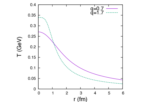
Figure 2: (Color online) The temperature profiles of the Gubser solutions for different values of the parameter $q$, at $\tau=0.6\ {\rm fm}$ as a function of $r$.

While we use Gubser solution for early evolution of the system, unfortunately it cannot be used all the way to freezeout. This solution was obtained by a conformal transformation and thus can only be used for conformal plasma with the conformal equation of state (EOS) $\epsilon=3p$. While it is believed to be a good approximation for the early QGP phase of the collision, this is certainly not the case near the QCD phase transition, where pressure $p$ remains roughly constant while the energy density $\epsilon$ changes by about an order of magnitude. Therefore, the initial Gubser-like stage is supplemented by a numerical hydro solution, based on the realistic lattice-based EOS. We therefore start from the Gubser solution, but then, at certain time $\tau_{0}=0.6\ {\rm fm}$, we switch to numerical evolution with the realistic EOS, derived from recent lattice QCD calculations Borsanyi et al. (2014).

(We recall the ideal relativistic hydrodynamic equations,

$$\partial_{\mu}T^{\mu\nu}=0,$$ (6)

where $T^{\mu\nu}$ is the energy-momentum tensor. For a perfect fluid, $T^{\mu\nu}$ can be expressed as

$$T^{\mu\nu}=(\epsilon+p)u^{\mu}u^{\nu}-p\eta^{\mu\nu},$$ (7)

where $\epsilon$ is the energy density, $p$ is the pressure, $u^{\mu}$ is the fluid four-velocity, and $\eta^{\mu\nu}\equiv\operatorname{diag}\{1,-1,-1,-1\}$ is the Minkowski metric. )

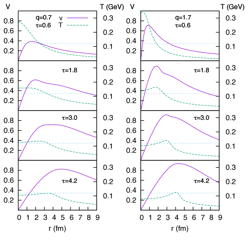
Figure 3: (Color online) Time evolutions of temperature and velocity for $q=0.7\ {\rm fm}^{-1}$ (left column) and $q=1.7\ {\rm fm}^{-1}$ (right column). Temperature (dashed line) and velocity (solid line) profiles at $\tau=0.6,1.8,3.0,4.2\ {\rm fm}$ are plotted as a function of the radial coordinate $r$. The dotted lines in the plots indicate the freezeout temperature $T_{\rm f}=0.12\ {\rm GeV}$.

II.2 Freezeout

In order to obtain the single-particle distribution from the hydrodynamic solutions, we use the standard Cooper-Frye formula Cooper and Frye (1974),

$$p^{0}\frac{d^{3}N}{d\eta dp_{T}^{2}}=\frac{1}{(2\pi)^{3}}\int\frac{p^{\mu}d\sigma_{\mu}(x)}{\exp\left[p\cdot u/T\right]\mp_{\rm BF}1}.$$ (8)

This formula is applied on a isothermal hypersurface characterized by the freezeout temperature $T_{\rm f}$. We perform Monte-Carlo sampling of pions according to the distribution (8), following the steps below:

1. Take a piece of surface elements $d\sigma^{\mu}$. We first calculated the average number of pions produced from this surface by

   $$dN=\frac{1}{(2\pi)^{3}}\int\frac{d^{3}p}{E}\frac{p^{\mu}d\sigma_{\mu}(x)}{\exp\left[p\cdot u/T\right]\mp_{\rm BF}1}.$$ (9)

2. Since $dN$ is typically a small number ($\sim 10^{-3}$), we can regard this number as a probability to produce a pion. According to this probability, we throw a dice and determine whether to make a pion or not. If we are to produce a pion, we sample the momentum of the pion from the distribution

   $$f_{1}(x,\bm{p})=\frac{1}{(2\pi)^{3}}\frac{p^{\mu}d\sigma_{\mu}(x)}{\exp\left[p\cdot u/T\right]\mp_{\rm BF}1}.$$ (10)

3. We repeat the steps 1 and 2 for all the freezeout surface elements.

We refer the reader to Ref. Hirano et al. (2013) for the details of the sampling procedures.

(a) $0.05\ {\rm GeV}<k_{\rm T}<0.15\ {\rm GeV}$

(b) $0.35\ {\rm GeV}<k_{\rm T}<0.45\ {\rm GeV}$

(c) $0.65\ {\rm GeV}<k_{\rm T}<0.75\ {\rm GeV}$

Figure 4: (Color online) Distribution of displacements in the out ($X_{\rm o}$) and side ($X_{\rm s}$) directions for $q=0.5\ {\rm fm}^{-1}$. Three figures are for different $k_{\rm T}$ bins.

(a) $0.05\ {\rm GeV}<k_{\rm T}<0.15\ {\rm GeV}$

(b) $0.35\ {\rm GeV}<k_{\rm T}<0.45\ {\rm GeV}$

(c) $0.65\ {\rm GeV}<k_{\rm T}<0.75\ {\rm GeV}$

Figure 5: (Color online) Distribution of displacements in the out ($X_{\rm o}$) and side ($X_{\rm s}$) directions for $q=1.5\ {\rm fm}^{-1}$.

II.3 Calculations of correlations

We have obtained the momenta and emission coordinates of produced pions from the sampling based on the Cooper-Frye formula. The effect of interference of identical particles is not included at this stage, since the Cooper-Frye formula gives us only a single-particle distribution function. The two-particle correlations come from Bose symmetrization

$$C(k_{\rm T},\bm{q})=\frac{\sum_{<i,j>\in[k_{\rm T}]}\left[1+\cos\left(q_{\mu}\Delta x^{\mu}\right)\right]}{\sum_{<i,j>\in[k_{\rm T}]}1},$$ (11)

where $\bm{k}_{\rm T}\equiv(\bm{p}_{1{\rm T}}+\bm{p}_{2{\rm T}})/2$ is the pair transverse momentum, $<i,j>\in[k_{\rm T}]$ indicates a pair of pions in a particular $k_{\rm T}$ bin, $q^{\mu}=p_{1}^{\mu}-p_{2}^{\mu}$ is four-momentum difference of a pion pair, and $\Delta x^{\mu}\equiv x_{1}^{\mu}-x_{2}^{\mu}$ is space-time distance of the pair. The correlation functions is evaluated in the “longitudinally comoving frame”, where $k_{z}=0$ for each pair. We impose a pseudo-rapidity cut $|\eta|<1.0$, by which the particles in the mid-rapidity region are selected.

We characterize the 3D correlation function in the “out-side-long” parametrization Pratt (1986); Bertsch et al. (1988),

$$C(k_{\rm T},\bm{q})=1+\lambda\exp\left[-R_{o}^{2}q_{o}^{2}-R_{s}^{2}q_{s}^{2}-R_{\ell}^{2}q_{\ell}^{2}\right],$$ (12)

where $R_{o,s,\ell}=R_{o,s,\ell}(k_{\rm T})$ are the HBT radii of interest in this study, $q_{o}$ is the component of momentum parallel to the pair transverse momentum, $q_{\ell}$ is the one parallel to the beam, and $q_{s}$ is the one perpendicular to out and long direction. For each $k_{\rm T}$ bin, we determined the values of HBT radii by $\chi^{2}$ fitting.

III Results

III.1 Time evolution of fireballs

The main qualitative feature of the solution is that the explosion is stronger for smaller (hotter) initial size – or larger values of Gubser parameter $q$. Quantitatively the time evolution of the temperature and radial flow velocity for $q=0.7\ {\rm fm}^{-1}$ (left column) and $q=1.7\ {\rm fm}^{-1}$ (right column) is shown in Fig. 3. The peak of the temperature in the central region $r\approx 0$ collapses, and the maximum moves to the rim of the fireball. While the pressure gradient pushes out the matter, the flow is increasing. One can see that the flow velocity reaches larger values for $q=1.7\ {\rm fm}^{-1}$, compared to the case with $q=0.7\ {\rm fm}^{-1}$. Freezeout surfaces are located at the intersections of the dashed lines (the fluid temperature) and the dotted line (the assumed value of the freezeout temperature), where fluid elements are turned into particles. At these intersections, the final flow is determined.

We again emphasize that while the absolute freezeout times in both cases displayed is similar ($\sim$ 4 fm), the flow magnitude is quite different. As expected, it is significanly larger for smaller fireballs, or larger $q$.

III.2 Flow and the distribution $P(\Delta x^{\mu})$

Hydrodynamics gives us an intuitive explanation of the $k_{\rm T}$ dependence, as mentioned in the Introduction. If one selects a larger value of $k_{\rm T}$, the relevant region where particles originate becomes smaller and more elliptic (see Fig. 1). This intuitive picture can be quantitatively checked by looking at the distribution, $P(\Delta x^{\mu})$, of the pair-displacement vector $\Delta x^{\mu}=x_{1}^{\mu}-x_{2}^{\mu}$ and its $k_{\rm T}$ dependence.

In Figs. 4 and Fig. 5, we show the probability distribution of the displacement in “out” and “side” directions, $P(X_{o},X_{s})$, for three $k_{\rm T}$ bins for two value of $q$ ($0.5\ {\rm fm}^{-1}$ and $1.5\ {\rm fm}^{-1}$). It is determined after the particle pairs are selected, from the Cooper-Frye integral over the freezeout surface. Here, $X_{o}$ is the projection of the displacement vector $\Delta x^{\mu}$ to the direction of $\bm{k}_{\rm T}$, and $X_{s}$ is the projection of $x^{\mu}$ in the direction perpendicular to $\bm{k}_{\rm T}$ and the beam axis. At low $k_{\rm T}$ [Fig. 4(a) and Fig. 5(a)], the distribution is broad and circular in out and side directions.

The wide circular component comes from the times when flow is still small, while a narrow strip comes from the region where it is substantial. For higher $k_{\rm T}$, the distribution is squeezed, and is narrower in the out direction compared to the side direction. These plots illustrate effect of the radial flow schematically shown in Fig. 1.

III.3 HBT radii

Now let us turn to the results of HBT radii. In Fig. 6, we show the HBT “volume“ ($R_{o}R_{s}R_{\ell}$) as a function of $k_{\rm T}$ for different values of $q$, together with the experimental data from ALICE. The parameter $\epsilon_{0}$ is chosen to match the observed multiplicity in ALICE. The radii from $q=1.5$ to $1.7\ {\rm fm}^{-1}$ reproduce the volume in the ALICE data well.

In Fig. 7, we show the ratio $R_{o}/R_{s}$ as a function of $k_{\rm T}$. Basically, $R_{o}/R_{s}$ is a decreasing function of $k_{\rm T}$. At small values of $q$, the slope of $R_{o}/R_{s}$ is gentle. As $q$ becomes larger, the slope becomes steeper and $R_{o}/R_{s}$ is suppressed at large $k_{\rm T}$. The ALICE data shows further suppression compared to the result from the largest value of $q$. Judging from the data, we can infer that $R_{o}/R_{s}$ is indicative of the strength of the flow. However, the reason why $R_{o}/R_{s}$ is suppressed at large $k_{\rm T}$ is not so trivial, which we explain in Sec. III.4.

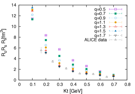
Figure 6: (Color online) HBT volume as a function of the pair transverse momentum $k_{\rm T}$ for various values of the parameter $q$. $dN_{\rm ch}/d\eta=27$, $T_{\rm f}=120\ {\rm MeV}$.

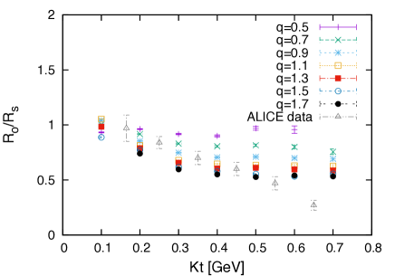
Figure 7: (Color online) The ratio $R_{o}/R_{s}$ as a function of $k_{\rm T}$ for various values of $q$. The initial size is more compressed for a larger $q$, which results in stronger radial flow at freezeout.

III.4 Why is the ratio $R_{o}/R_{s}$ most sensitive to the strength of radial flow?

Here we discuss the reason why $R_{o}/R_{s}$ is suppressed at large $k_{\rm T}$ in the presence of a strong radial flow. Depending on the $k_{\rm T}$ cut, the area where particles originate changes. As $k_{\rm T}$ becomes higher, the region shrinks, especially in the outward direction. If the system is composed of a gas with a large mean free path, such a behavior would not be present. This trend indicates that the system is strongly interacting. Furthermore, we claim that the ratio $R_{o}/R_{s}$ is sensitive to the strength of the flow. What is difficult to understand is that, if one looks at the distribution itself, $P(\Delta x^{\mu})$, the ratio of the widths of out and side directions, $L_{o}/L_{s}$, does not appear to be different for different values $q$ (compare Figs. 4 and 5).

This might seem to be inconsistent with the behavior of $R_{o}/R_{s}$ at large $k_{\rm T}$ calculated from the fitted radii: the ratio is almost unity at weak flow case ($q=0.7\ {\rm fm}^{-1}$), and it decreases as $q$ gets larger. Below we explain the reason for the apparent discrepancy. We will find that the suppression of the ratio $R_{o}/R_{s}$ at large $k_{\rm T}$ for the strong flow case is mainly driven by correlation of emission time difference and distance of the emitted points in the out direction. This was first pointed out in Ref. Borysova et al. (2006) and is consistent with results in Ref. Kisiel (2011), in which the HBT radii for $pp$ collisions are studied using a blast-wave model.

We consider the quantities

$$\left.\frac{\partial^{2}C(k_{\rm T},\bm{q})}{\partial q_{i}\partial q_{j}}\right|_{\bm{q}=0},$$ (13)

where $i,j\in\{t,o,s,\ell\}$. When $P(\Delta x^{\mu})$ is approximated by a Gaussian form,

$$P(\Delta x^{\mu})=\frac{1}{16\pi^{2}V}\exp\left[-\frac{X_{t}^{2}}{4L_{t}^{2}}-\frac{X_{o}^{2}}{4L_{o}^{2}}-\frac{X_{s}^{2}}{4L_{s}^{2}}-\frac{X_{\ell}^{2}}{4L_{\ell}^{2}}\right],$$ (14)

where $L_{t,o,s,l}$ are the widths in time, out, side, and long directions, and $V\equiv L_{t}L_{o}L_{s}L_{\ell}$, the HBT radii can be expressed by the moments as

$$R_{i}^{2}=\left.\frac{\partial^{2}C(k_{\rm T},\bm{q})}{\partial q_{i}^{2}}\right|_{\bm{q}=0},$$ (15)

with $i\in\{o,s,\ell\}$.

Below we express the measured HBT radii in terms of the moments the distribution $P(\Delta x^{\mu})$. The two-particle correlation function reads

$$\begin{split}C(k_{\rm T},\bm{q})-1&=\int dX_{t}dX_{o}dX_{s}dX_{\ell}\ P(\Delta x^{\mu})\cos\left(q_{\mu}\Delta x^{\mu}\right)\\ &=\mathop{\mathrm{Re}}\left[\int dX_{t}dX_{o}dX_{s}dX_{\ell}\ P(\Delta x^{\mu})e^{iq_{\mu}\Delta x^{\mu}}\right].\end{split}$$ (16)

The exponent in the integral can be written as

$$\begin{split}q_{\mu}\Delta x^{\mu}&=q_{0}X_{t}-\bm{q}\cdot\Delta\bm{x}\\ &=\bm{\beta}\cdot\bm{q}\ X_{t}-\bm{q}_{\rm T}\cdot\Delta\bm{x}_{\rm T}\\ &=(\beta_{\rm T}q_{o}+\beta_{\rm L}q_{\ell})X_{t}-q_{o}X_{o}-q_{s}X_{s}-q_{\ell}X_{\ell},\end{split}$$ (17)

where $\bm{\beta}=\bm{k}/k_{0}$ and we used $\beta_{s}=0$ ($\bm{\beta}$ is parallel to $\bm{k}$), and $q_{0}=\bm{\beta}\cdot\bm{q}$ ($\leftrightarrow k_{\mu}q^{\mu}=0$), and $\beta_{\rm T}$ and $\beta_{\rm L}$ are the projections of $\bm{\beta}$ in transverse and longitudinal directions. In the current case, where the correlations function is evaluated in the frame with $k_{z}=0$, $\beta_{\rm T}=\beta$ and $\beta_{\rm L}=0$. Thus, the HBT radii and the moments are related by

$$R_{o}^{2} = \left<\left(X_{o}-\beta X_{t}\right)^{2}\right>$$ (18)

$$= \left<X_{o}^{2}\right>+\left<\beta^{2}X_{t}^{2}\right>-2\left<\beta X_{t}X_{o}\right>,$$

$$R_{s}^{2} = \left<X_{s}^{2}\right>,$$ (19)

$$R_{\ell}^{2} = \left<X_{\ell}^{2}\right>.$$ (20)

Indeed, one can see that the radii calculated from the moments, using Eqs. (18), (19) and (20), shows consistent behavior with the ones obtained by fitting procedure, compare Figs. 8 and 7.

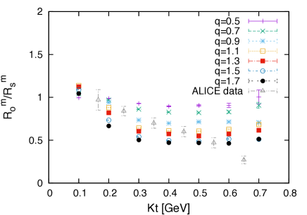
Figure 8: (Color online) $R_{o}/R_{s}$ calculated from the moments.

Now let us discuss the reason why $R_{o}/R_{s}$ is suppressed at large $k_{\rm T}$ in the presence of strong flow. In terms of the ratio of moments, $R_{o}/R_{s}$ is composed of three terms,

$$\frac{R_{o}^{2}}{R_{s}^{2}}=\frac{\left<X_{o}^{2}\right>}{\left<X_{s}^{2}\right>}+\frac{\left<\beta^{2}X_{t}^{2}\right>}{\left<X_{s}^{2}\right>}-2\frac{\left<\beta X_{t}X_{o}\right>}{\left<X_{s}^{2}\right>},$$ (21)

In order to see which term plays the dominant role in the suppression of $R_{s}/R_{o}$ for strong flow, we plotted the values of each term for different values of the Gubser parameter $q$, as a function of $k_{\rm T}$ (Figs. 9, 10, and 11 ). The behavior of the first term $\left<X_{o}^{2}\right>/\left<X_{s}^{2}\right>$ is shown in Fig. 9. For all the values of $q$, the ratio is around $1$ at lowest $k_{\rm T}$, and is less than unity at higher $k_{\rm T}$. Note the fact that, at highest $k_{\rm T}$, the ratio is more suppressed for weaker flows. This indicates that the suppression of $R_{o}/R_{s}$ at large $k_{\rm T}$ for a strong flow is not caused by the term $\left<X_{o}^{2}\right>/\left<X_{s}^{2}\right>$.

The suppression of $R_{o}/R_{s}$ is driven by $\left<\beta X_{t}X_{o}\right>/\left<X_{s}^{2}\right>$, which is shown in Fig. 11. This term is a measure of correlation between emission time difference and the displacement in the out direction. For a weak flow (small $q$), it is close to zero and the correlation is weak for the entire region of $k_{\rm T}$. As we go to stronger flow (larger $q$), the lines rises and the correlation at high $k_{\rm T}$ becomes stronger. Since this term contributes to $R_{o}/R_{s}$ with a negative sign, it leads to the suppression of $R_{o}/R_{s}$ at large $k_{\rm T}$.

Figure 9: (Color online) $\left<X_{o}^{2}\right>/\left<X_{s}^{2}\right>$ as a function of $k_{\rm T}$.

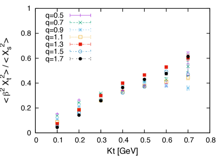
Figure 10: (Color online) $\left<\beta^{2}X_{t}^{2}\right>/\left<X_{s}^{2}\right>$ as a function of $k_{\rm T}$.

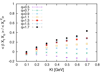
Figure 11: (Color online) $\left<\beta X_{t}X_{o}\right>/\left<X_{s}^{2}\right>$ as a function of $k_{\rm T}$.

IV Summary

ALICE HBT data Aggarwal et al. (2011) provided a striking indication that the highest multiplicity bin of $pp$ collisions at the LHC is rather different from others: it shows evidence of strong radial flow. We performed simulations of the system, using ideal relativistic hydrodynamics. The early evolution is described by a Gubser conformal solution, complemented by a numerical one, with a realistic EOS at later stages. We show how strength of the radial flow depends on the initial size and temperature of the fireball.

Comparison of the resulting HBT radii with high multiplicity data shows the best agreement only for the smallest fireball we study, with Gubser parameter $q=1.5-1.7\ {\rm fm}^{-1}$. It confirms that one in fact observes the presence of collective hydrodynamical flow in an unprecedented small system, smaller than 1 fm initially.