Space-time adaptive ADER discontinuous Galerkin finite element schemes with a posteriori sub-cell finite volume limiting

Abstract

In this paper we present a novel arbitrary high order accurate discontinuous Galerkin (DG) finite element method on space-time adaptive Cartesian meshes (AMR) for hyperbolic conservation laws in multiple space dimensions, using a high order a posteriori sub-cell ADER-WENO finite volume limiter. Notoriously, the original DG method produces strong oscillations in the presence of discontinuous solutions and several types of limiters have been introduced over the years to cope with this problem. Following the innovative idea recently proposed in [53], the discrete solution within the troubled cells is recomputed by scattering the DG polynomial at the previous time step onto a suitable number of sub-cells along each direction. Relying on the robustness of classical finite volume WENO schemes, the sub-cell averages are recomputed and then gathered back into the DG polynomials over the main grid. In this paper this approach is implemented for the first time within a space-time adaptive AMR framework in two and three space dimensions, after assuring the proper averaging and projection between sub-cells that belong to different levels of refinement. The combination of the sub-cell resolution with the advantages of AMR allows for an unprecedented ability in resolving even the finest details in the dynamics of the fluid. The spectacular resolution properties of the new scheme have been shown through a wide number of test cases performed in two and in three space dimensions, both for the Euler equations of compressible gas dynamics and for the magnetohydrodynamics (MHD) equations.

1 Introduction

The numerical solution of hyperbolic problems has attracted a lot of attention in recent years, as they arise in many physical and technological applications. Many of them are in the field of computational fluid dynamics, such as compressible gas dynamics, multiphase flows, air flow around aircraft or cars, astrophysical flows, free surface flows, environmental and geophysical flows like avalanches, dam break problems and water flow in channels, rivers and oceans, to mention but a few. Among the numerical methods specifically developed to solve hyperbolic problems, there are finite volume (FV) methods and discontinuous Galerkin (DG) methods. While until a few years ago FV methods were comparatively more popular, the situation is now rapidly changing and DG schemes, first introduced by Reed and Hill in [105] to solve a first order neutron transport equation, are now widely applied in several different fields, in particular those related to fluid dynamics. In a series of masterpiece works [31, 30, 29, 28, 32], Cockburn and Shu provided a rigorous formal framework of these methods, contributing significantly to their widespread use. DG methods are very robust and, among high order numerical methods, they show high flexibility and adaptivity strategies in handling complex geometries [104]. Moreover, Jiang and Shu proved in [74] that DG methods verify an entropy condition which confers them nonlinear $L_{2}$ stability. Despite this interesting property, explicit DG methods have a strong stability limitation, since usually the CFL restriction for these schemes is very severe and the time step in $d$ space dimensions is constrained as $\Delta t\leq h/[d(2N+1)|\lambda_{max}|]$, where $d$ is the number of space dimensions, $h$ is a characteristic mesh size, $\lambda_{max}$ is the maximum signal velocity and $N$ is the degree of the basis polynomial.

In DG schemes a high order time integration is typically performed by means of TVD Runge-Kutta schemes [64], leading to the family of so-called RKDG schemes. These methods are certainly efficient, but they have a maximum reachable order of accuracy in time, which is four. However, due to the high complexity of the fourth order TVD Runge-Kutta scheme, only up to third order TVD Runge-Kutta methods are used in practice. In the presence of stiff source terms, usually the so-called IMEX Runge-Kutta schemes are employed, see [96, 97]. To overcome these limitations, in our approach we follow the so-called ADER strategy for time integration, which was first introduced by Toro and Titarev in the finite volume context [118, 113, 119, 115, 116], and it is a very attractive tool allowing to achieve arbitrary order of accuracy in space and time in one single step by incorporating the approximate solution of a Generalised Riemann Problem (GRP) at the element interfaces. There are essentially two different families of approximate GRP solvers: those who first interact the spatial derivatives and subsequently compute a temporal expansion at the interface [14, 57, 19, 118, 113, 119, 115, 116, 47], and those who first evolve the data locally in the small inside each element and then interact the evolved data at the element interfaces via a classical Riemann solver, see e.g. [65, 90, 60, 43, 51, 41]. For a more detailed discussion on the approximate solution of the GRP, see [23, 94, 63]. Nevertheless, the original ADER approach has two main drawbacks: first, it makes use of the rather cumbersome and problem-dependent Cauchy-Kowalewski procedure and, second, it fails in the presence of stiff source terms. A subsequent version of the ADER approach that solves both these difficulties was developed in [43], where the Cauchy-Kowalewski procedure was replaced with a local space-time DG predictor approach based on a weak formulation of the problem in space-time. This formulation is usually referred to as the local space-time discontinuous Galerkin (LSTDG) predictor and it has been successfully adopted in a variety of mathematical and physical problems [51, 67, 40, 52, 44, 10]. We remark that, although this LSTDG approach is locally implicit, the full formulation remains explicit and, therefore, the above mentioned CFL restriction still holds. The ADER time stepping method has been also applied successfully to the discontinuous Galerkin finite element framework, see e.g. [47, 100, 46].

DG schemes are very efficient in smooth regions, but in the presence of sharp gradients and/or shock waves, they cannot escape from the Gibbs phenomenon and, as a consequence, they give rise to undesirable oscillations in the solution, since they are linear in the sense of Godunov. In fact, according to Godunov’s theorem [62] there are no linear and monotone schemes of order higher than the first. In the finite volume framework Godunov’s theorem is circumvented by carrying out a nonlinear reconstruction within each cell. Here, TVD slope limiters [117] and ENO/WENO reconstructions [65, 75, 5, 114] are among the most popular. In the discontinuous Galerkin approach, on the other hand, even if in principle no spatial reconstruction is needed, in practice it is necessary to introduce some sort of limiters to avoid oscillations in the presence of discontinuities. Among the most relevant limiters proposed so far we mention the use of artificial viscosity [66, 98, 26, 56, 38, 55], of spectral filtering [103], of (H)WENO limiting procedures [102, 101, 77, 4, 78, 79, 68], and of slope and moment limiting [30, 88, 104, 1, 125, 37]. In [53] we have recently proposed a totally different and alternative solution to this longstanding problem, which relies on a new a posteriori sub-cell finite volume limiting approach. In practice, we first compute the solution by means of an unlimited DG scheme, and subsequently we find the troubled cells by using some very simple but effective a posteriori detection criteria, namely the positivity of the solution and a relaxed discrete maximum principle in the sense of polynomials. Once the troubled cells have been identified, a sub-grid of size $(2N+1)^{d}$ is created within these cells and a more robust ADER-WENO finite volume approach is used to recompute the solution on the subgrid. A peculiar aspect of this new paradigm is that the size of the sub-grid is chosen as to make sure that the maximum admissible time step of the finite volume scheme on the sub-cells matches the time step of the DG scheme on the main grid. The idea of introducing an a posteriori approach to the problem of limiting has been recently established by Clain, Diot and Loubère in the finite volume context, by means of the so-called Multi-dimensional Optimal Order Detection (MOOD) method [27, 35, 36, 91]. The MOOD paradigm may in fact be considered as the progenitor of our a posteriori limiting procedure for DG schemes [53].

In the present work we combine the new ADER-DG paradigm with a posteriori subcell limiters of [53] with Adaptive Mesh Refinement (AMR) techniques, thus significantly enhancing the resolution capabilities compared to simple uniform grids. AMR was first proposed by M. J. Berger and collaborators in a series of well-known papers [17, 15, 18]. They introduced a patch-boxed block-structured AMR approach developed within the finite volume framework and later used extensively for astrophysical applications. Other interesting developments have been presented in [3], where the first higher order AMR algorithms based on WENO finite volume schemes have been introduced. Applications of AMR techniques in the field of shallow water equations have been reported, for instance, by [39]. Other interesting implementations of adaptive mesh refinement are based on the so-called quadtree/octree refinement; for an overview of these techniques in different contexts see [2] and [121]. AMR techniques have also been successfully implemented with Central WENO (CWENO) schemes, such as in [72, 73]. Following the ”cell-by-cell”’ refinement approach of [80], the first implementation of a high order ADER-WENO finite volume scheme with AMR was proposed in [52, 44] for conservative and nonconservative hyperbolic PDE in two and three space dimensions. It was subsequently extended to special relativistic hydrodynamics (RHD) and magnetohydrodynamics (RMHD) in [128].

The combination of DG schemes with AMR has been considered in a significant number of papers, although in this context the concept of adaptive mesh refinement is commonly absorbed into that of hp-adaptivity. Two well-known early series of papers on hp-adaptive DG schemes are due to Baumann and Oden [13, 12] and Houston, Süli and Schwab, see [70, 69, 71]. Furthermore, in [86] a DG scheme was proposed with anisotropic AMR for the compressible Navier–Stokes equations, while in [93, 126] the Euler equations have been solved on adaptive unstructured meshes. In the context of atmospheric simulations, on the other hand, [81] implemented a numerical scheme which includes implicit-explicit RKDG, artificial viscosity and adaptive mesh refinement on two dimensional non-conforming elements. Other relevant results have been obtained in [61], [92]. Our goal is to improve with respect to these approaches by proposing a space-time adaptive ADER-DG scheme with time-accurate local time stepping that can be arbitrarily high order accurate both in space and time, that avoids Runge–Kutta sub-steps as well as artificial viscosity of any kind, and that incorporates a proper a posteriori subcell limiter within the full advantages of AMR.

The plan of the paper is the following: in Section 2 we present the basic mathematical framework, while in Section 3 we explain the ADER discontinuous Galerkin method. Section 4 is devoted to the description of the a posteriori sub-cell limiter, whereas the incorporation within the AMR framework is deferred to Section 5. The numerical results are discussed in Section 6 and the conclusions are given in Section 7.

2 Mathematical framework: an overview

We consider nonlinear systems of hyperbolic equations written in conservative form as

$$\frac{\partial\mathbf{u}}{\partial t}+\nabla\cdot\mathbf{F}\left(\mathbf{u}\right)=0,\qquad\mathbf{x}\in\Omega\subset\mathds{R}^{d},\quad t\in\mathds{R}_{0}^{+},$$ (1)

where $\mathbf{u}$ is the vector of so-called conserved quantities, while $\mathbf{F}(\mathbf{u})=(\mathbf{f},\mathbf{g},\mathbf{h})$ is a non-linear flux tensor that depends on the state $\mathbf{u}$. The computational domain $\Omega$ is discretized by a Cartesian grid composed by elements $T_{i}$, namely

$$\Omega=\bigcup\limits_{i=1}^{N_{E}}T_{i}\,,$$ (2)

where the index $i$ ranges from 1 to the total number of elements $N_{E}$, which, in our adaptively mesh refinement framework, is of course a time-dependent quantity. In the following, we denote the cell volume by $|T_{i}|=\int_{T_{i}}d\mathbf{x}$. At the beginning of each time-step, the numerical solution of Eq.  (1) is represented within each cell $T_{i}$ by piecewise polynomials of maximum degree $N\geq 0$ as

$$\mathbf{u}_{h}(\mathbf{x},t^{n})=\sum_{l=0}^{N}\Phi_{l}(\mathbf{x})\hat{\mathbf{u}}^{n}_{l}=\Phi_{l}(\mathbf{x})\hat{\mathbf{u}}^{n}_{l}\quad\mathbf{x}\in T_{i}\,,$$ (3)

where $\mathbf{u}_{h}$ is referred to as the discrete representation of the solution, while the coefficients $\hat{\mathbf{u}}^{n}_{l}$ are usually called the degrees of freedom. In the expansion expressed by Eq. (3), the basis functions $\Phi_{l}(\mathbf{x})$ are chosen as tensor-products of Lagrange interpolation polynomials of maximum degree $N$ which pass through the tensor-product of $(N+1)$ Gauss-Legendre quadrature points [109, 82, 59, 83].
The numerical method used in this paper is the combination of several crucial steps, which will be described below and that can be listed schematically as

• a predictor step, in which Eq. (1) is solved within each element in the small [65] by means of a locally implicit space-time discontinuous Galerkin scheme (see Sect. 3.1);

• a pure discontinuous Galerkin (DG) scheme, i.e. a $\mathbb{P}_{N}\mathbb{P}_{N}$ scheme according to [41], which, by exploiting the information obtained by the predictor, allows to compute the solution at the next time level through a single one-step corrector (see Sect. 3.2);

• an a posteriori sub-cell limiter, which recomputes the solution of the troubled cells needing a limiter through an ADER-WENO finite volume scheme acting at the sub-cell level (see Sect. 4);

• an adaptive mesh refinement (AMR) approach, which is implemented according to a cell-by-cell strategy and must be properly nested within the sub-cell philosophy (see Sect. 5).

We emphasize that the adaptivity of the main grid provided by the AMR approach has nothing to do with the subcell limiter. The AMR technology is used to refine and recoarsen the computational grid according to physical features that one wants to follow, while the subgrid limiter is only used to cope with shock waves or other discontinuities that require limiting of the DG scheme. In the following we provide the necessary minimum details for each of the above items, while addressing the reader to [41, 51, 67, 58, 11, 52, 53] for an exhaustive discussion of the subtleties that may be involved.

3 The ADER-DG scheme

3.1 The local space-time predictor

At the heart of the ADER approach, either in the original version proposed in [113] and [115] or in the later version proposed in [43, 41, 11], that we also follow in this paper, there is the solution of the generalised or derivative Riemann problem. This requires a time evolution of known spatial derivatives of the polynomials approximating the solution at time $t^{n}$ and is in our case performed locally for each cell and independently from the neighbor cells. In the FV framework, such polynomials are obtained via reconstruction from the known cell averages of the conserved quantities. In the DG framework, on the contrary, no reconstruction is needed and the time evolution acts directly on the representation polynomials $\mathbf{u}_{h}(\mathbf{x},t^{n})$ of Eq. (3). To show how the predictor works, we first transform the PDE system of Eq. (1) into a space-time reference coordinate system $(\xi,\eta,\zeta,\tau)$. In practice, the space-time control volume $\mathcal{C}_{ijkn}=[x_{i-\frac{1}{2}};x_{i+\frac{1}{2}}]\times[y_{j-\frac{1}{2}};y_{j+\frac{1}{2}}]\times[z_{k-\frac{1}{2}};z_{k+\frac{1}{2}}]\times[t^{n};t^{n+1}]$ is mapped into the space-time reference element $[0;1]^{4}$ through the definitions

$$x=x_{i-\frac{1}{2}}+\xi\Delta x_{i},\quad y=y_{j-\frac{1}{2}}+\eta\Delta y_{j},\quad z=z_{k-\frac{1}{2}}+\zeta\Delta z_{k},\quad t=t^{n}+\tau\Delta t\,.$$ (4)

In general, we will use $T_{E}=[0;1]^{d}$ to denote the spatial reference elements in $d$ spatial dimensions. As a result, Eq. (1) will be rewritten as

$$\frac{\partial\mathbf{u}}{\partial\tau}+\nabla_{\xi}\cdot\mathbf{F}^{*}\left(\mathbf{u}\right)=0,$$ (5)

where

$$\mathbf{F}^{*}:=\Delta t\left(\partial\bm{\xi}/\partial\mathbf{x}\right)^{T}\cdot\mathbf{F}(\mathbf{u})$$ (6)

with $(\bm{\xi}=\xi,\eta,\zeta)$ and $\nabla_{\xi}=\partial\bm{\xi}/\partial\mathbf{x}\cdot\nabla$. Multiplication of (5) with a space-time test function $\theta_{k}=\theta_{k}(\bm{\xi},\tau)$ and integration over the space-time reference control volume $T_{E}\times[0;1]$ yields

$$\int\limits_{0}^{1}\int\limits_{T_{E}}\theta_{k}\frac{\partial\mathbf{u}}{\partial\tau}\,d\bm{\xi}\,d\tau\,+\int\limits_{0}^{1}\int\limits_{T_{E}}\theta_{k}\nabla_{\xi}\cdot\mathbf{F}_{h}^{*}\left(\mathbf{u}\right)\,d\bm{\xi}\,d\tau\,=0\,.$$ (7)

In analogy to Eq. (3), we now introduce the discrete spacetime solution of equation (7), denoted by $\mathbf{q}_{h}$, as well as the corresponding one for the flux, i.e.

$$\mathbf{q}_{h}=\mathbf{q}_{h}(\bm{\xi},\tau)=\theta_{l}\hat{\mathbf{q}}_{l}\,.$$ (8)

$$\mathbf{F}^{*}_{h}=\mathbf{F}^{*}_{h}(\bm{\xi},\tau)=\theta_{l}\hat{\mathbf{F}}^{*}_{l},$$ (9)

The space-time test and basis functions $\theta_{l}$ are chosen again as tensor products of Lagrange interpolation polynomials passing through the Gauss-Legendre quadrature points. Due to this choice of a nodal basis, the degrees of freedom for the fluxes are simply the point–wise evaluation of the physical fluxes, namely

$$\hat{\mathbf{F}}^{*}_{l}=\mathbf{F}^{*}(\hat{\mathbf{q}}_{l})\,.$$ (10)

The next crucial step of the approach consists of integrating by parts in time the first term in (7), while keeping the information local in space. This yields

$$\int\limits_{T_{E}}\theta_{k}(\bm{\xi},1)\mathbf{q}_{h}\,d\bm{\xi}-\int\limits_{T_{E}}\theta_{k}(\bm{\xi},0)\mathbf{u}_{h}\,d\bm{\xi}-\int\limits_{0}^{1}\int\limits_{T_{E}}\frac{\partial\theta_{k}}{\partial\tau}\mathbf{q}_{h}\,d\bm{\xi}\,d\tau+\int\limits_{0}^{1}\int\limits_{T_{E}}\theta_{k}\nabla_{\xi}\cdot\mathbf{F}^{*}_{h}\,d\bm{\xi}\,d\tau=0.$$ (11)

After substituting (8) and (9) into Eq. (11) we obtain [41, 67, 51]

$$\left(\int\limits_{T_{E}}\theta_{k}(\bm{\xi},1)\theta_{l}(\bm{\xi},1)\,d\bm{\xi}-\int\limits_{0}^{1}\int\limits_{T_{E}}\frac{\partial\theta_{k}}{\partial\tau}\theta_{l}\,d\bm{\xi}\,d\tau\right)\hat{\mathbf{q}}_{l}=\left(\int\limits_{T_{E}}\theta_{k}(\bm{\xi},0)\Phi_{l}\,d\bm{\xi}\right)\hat{\mathbf{u}}_{l}^{n}-\left(\int\limits_{0}^{1}\int\limits_{T_{E}}\theta_{k}\nabla_{\xi}\theta_{l}\,d\bm{\xi}\,d\tau\right)\mathbf{F}^{*}(\hat{\mathbf{q}}_{l})\,.$$ (12)

Equations (12) represents a nonlinear system to be solved in the unknown expansion coefficients $\hat{\mathbf{q}}_{l}$ of the local space-time predictor solution, while the terms $\hat{\mathbf{u}}_{l}^{n}$ are the known degrees of freedom of the DG polynomial at time level $t^{n}$. We note, incidentally, that, although the solution of the above nonlinear system is certainly demanding in terms of computational costs, it has the significant advantage that it can also cope with stiff source terms, which are absent for the system of equations considered in this paper but are quite common in several fields of applied mathematics and physical sciences [51, 67, 127, 50].

3.2 The fully discrete one-step ADER-DG scheme

The spacetime solution $\mathbf{q}_{h}$ of Eq. (12) cannot of course provide the true solution at time level $t^{n+1}$, since it completely neglects the contribution of fluxes from neighbouring cells. In our approach, the proper correction is obtained through a fully discrete one-step ADER-DG scheme, which works as follows (see also [47, 110, 100]). We first multiply the governing PDE (1) by a test function $\Phi_{k}$, identical to the spatial basis functions of Eq. (3). Second, we integrate over the space-time control volume $T_{i}\times[t^{n};t^{n+1}]$. The flux divergence term is then integrated by parts in space, thus yielding

$$\int\limits_{t^{n}}^{t^{n+1}}\int\limits_{T_{i}}\Phi_{k}\frac{\partial\mathbf{u}_{h}}{\partial t}d\mathbf{x}dt+\int\limits_{t^{n}}^{t^{n+1}}\int\limits_{\partial T_{i}}\Phi_{k}\,\mathbf{F}\left(\mathbf{u}_{h}\right)\cdot\mathbf{n}\,dSdt-\int\limits_{t^{n}}^{t^{n+1}}\int\limits_{T_{i}}\nabla\Phi_{k}\cdot\mathbf{F}\left(\mathbf{u}_{h}\right)d\mathbf{x}dt=0,$$ (13)

where $\mathbf{n}$ is the outward pointing unit normal vector on the surface $\partial T_{i}$ of element $T_{i}$. Since the discrete solution is allowed to be discontinuous at element boundaries, the surface integration involved in the second term of (13) is done through the solution of a Riemann problem, which is therefore deeply rooted in the DG scheme and guarantees the overall upwind character of the method [31, 30, 29, 28, 32]. Whatever numerical flux function (Riemann solver) is chosen, denoted as $\mathcal{G}$, the time integration of the second and of the third term of Eq. (13) must be performed to the desired order of accuracy. To this extent, we use the local space-time predictor $\mathbf{q}_{h}$ from Sect. 3.1, which clearly pays off at this stage, and allows to compute the numerical flux function of the second term as $\mathcal{G}\left(\mathbf{q}_{h}^{-},\mathbf{q}_{h}^{+}\right)$ and the physical flux of the third term as $\mathbf{F}\left(\mathbf{q}_{h}\right)$. We emphasize that $\mathbf{q}_{h}^{-}$ and $\mathbf{q}_{h}^{+}$ are the left and right states of the Riemann problem. On the other hand, after inserting $\mathbf{u}_{h}$, as given by (3), in the first term of (13) we find the following arbitrary high order accurate one-step discontinuous Galerkin (ADER-DG) scheme:

$$\left(\int\limits_{T_{i}}\Phi_{k}\Phi_{l}d\mathbf{x}\right)\left(\hat{\mathbf{u}}_{l}^{n+1}-\hat{\mathbf{u}}_{l}^{n}\right)+\int\limits_{t^{n}}^{t^{n+1}}\int_{\partial T_{i}}\Phi_{k}\,\mathcal{G}\left(\mathbf{q}_{h}^{-},\mathbf{q}_{h}^{+}\right)\cdot\mathbf{n}\,dSdt-\int\limits_{t^{n}}^{t^{n+1}}\int_{T_{i}}\nabla\Phi_{k}\cdot\mathbf{F}\left(\mathbf{q}_{h}\right)d\mathbf{x}dt=0\,.$$ (14)

Concerning the choice of the Riemann solver, in this paper we have used both the simple Rusanov flux [106], and the more sophisticated Osher-type flux proposed in [49], which requires the knowledge of the eigenvectors of the system (1). For a very recent alternative family of genuinely multi-dimensional HLL Riemann solvers, see [7, 8, 9, 10].

The effective order of accuracy of the ADER-DG scheme resulting from (14) is $N+1$, both in space and in time, as long as the solution remains smooth. In spite of its great ability in achieving sub-cell resolution even on very coarse grids, the ADER-DG scheme, as well any other unlimited DG scheme, will fail at discontinuities due to the Gibbs phenomenon. For this reason it is necessary to introduce some sort of limiter, which should ideally preserve the typical sub-cell resolution properties of the DG method. Such an approach, proposed and discussed with all details in [53], is briefly summarized in the next section. Before proceeding, we also comment on the Courant-Friedrichs-Lewy (CFL) restriction imposed by explicit DG schemes. In multiple space dimensions, the time step is usually restricted as [84]

$$\Delta t<\frac{1}{d}\frac{1}{(2N+1)}\frac{h}{|\lambda_{\max}|}\,,$$ (15)

where $d$ is the number of space dimensions, $h$ and $|\lambda_{\max}|$ are a characteristic mesh size and the maximum signal velocity, respectively. The factor $2N+1$ in the denominator of (15) will motivate the choice for the number of sub-cells required by the limiter, as we explain below. Note that for ADER-DG schemes and Lax-Wendroff DG schemes, the CFL condition is even slightly more severe, see [41, 100].

4 A posteriori sub-cell limiter

Let us assume that we have obtained the discrete representation $\textbf{u}_{h}(\textbf{x},t^{n})$, within a general cell $T_{i}$, of the solution. In order to update the solution to the next time level, we first calculate a so-called candidate solution, denoted so forth as $\textbf{u}_{h}^{*}(\textbf{x},t^{n+1})$, which results from the unlimited scheme of Eq. (14). Due to the appearance of possible oscillations, the candidate solution may not be acceptable everywhere in the computational domain, and a number of detection criteria must be fulfilled in order to promote the candidate solution to the accepted discrete solution at the new time level. The first criterion is based on physical considerations and it consists of checking whether $\textbf{u}_{h}^{*}(\textbf{x},t^{n+1})$ verifies the physical positivity constraints. This is a necessary condition for a number of variables appearing in many conservation laws (mass, density, pressure, internal energy, water depth, etc.). For simplicity, and because this will be the case in the rest of the paper, we can refer to the Euler equations for gas dynamics, for which density and pressure must remain positive. Since the DMP was already a very useful tool to construct high resolution shock capturing finite volume schemes in the past, our second detection criterion is a relaxed discrete maximum principle (DMP) in the sense of polynomials. To this purpose, the following condition must be verified

$$\min\limits_{y\in{\cal{V}}_{i}}(\textbf{u}_{h}(\textbf{y},t^{n}))-\delta\leq\textbf{u}_{h}^{*}(\textbf{x},t^{n+1})\leq\max\limits_{\textbf{y}\in{\cal{V}}_{i}}(\textbf{u}_{h}(y,t^{n}))+\delta,\qquad\forall\textbf{x}\in T_{i}\,,$$ (16)

where the set ${\cal{V}}_{i}$ contains the cell $T_{i}$ and the Voronoi neighbor cells which share a common node with $T_{i}$. In practice, Eq. (16) says that the polynomial representing the candidate solution must lie between the minimum and the maximum of the polynomials representing the solution at the previous time step in the set ${\cal{V}}_{i}$. The small quantity $\delta$ in (16) is used to relax the maximum principle thus allowing for small undershoots and overshoots and it can avoid problems with roundoff errors. The value used here, as recommended in [53], is

$$\delta=\max\left(\delta_{0},\epsilon\cdot\left(\max\limits_{y\in{\cal{V}}_{i}}(\textbf{u}_{h}(y,t^{n}))-\min\limits_{y\in{\cal{V}}_{i}}(\textbf{u}_{h}(\textbf{y},t^{n}))\right)\,\right),$$ (17)

with $\delta_{0}=10^{-4}$ and $\epsilon=10^{-3}$. It is interesting to remark that the physical and the numerical criteria are totally independent, which implies that the relaxation of the maximum principle does not affect the positivity of the solution. Moreover, this approach takes into account the information from two different time levels, $t^{n}$ and $t^{n+1}$, whereas classical indicators typically use information from one time level only.

During the detection phase, if either the first physical criterion or the second numerical criterion is not fulfilled, the corresponding cell will acquire a so-called limiter status $\beta=1$, which flags the cell as troubled. On the other hand, if both criteria are met, the limiter status is set to $\beta=0$. Troubled cells immediately generate a sub-grid, for which an alternative data representation $\textbf{v}_{h}(\textbf{x},t^{n})$ must be provided. This new solution is expressed by a set of piecewise constant sub-cell averages $\textbf{v}_{i,j}^{n}$. These values are computed via $L_{2}$ projection on the $(N_{s})^{d}$ sub-cells $S_{i,j},j=1,\cdots,(N_{s})^{d}$ in which $T_{i}$ is divided, where $N_{s}=2N+1$, i.e.

$$v_{i,j}^{n}=\frac{1}{|S_{i,j}|}\int_{S_{i,j}}{\textbf{u}_{h}(\textbf{x},t^{n})\,d\textbf{x}}=\frac{1}{|S_{i,j}|}\int_{S_{i,j}}{\hat{\textbf{u}}_{l}^{n}\phi_{l}(\textbf{x})\,d\textbf{x}},\qquad\forall S_{i,j}\in{\cal{S}}_{i}\,,$$ (18)

and where ${\cal{S}}_{i}=\bigcup_{j}S_{i,j}$ is the set of the sub-grid cells. We emphasize that the choice $N_{s}=2N+1$ is not a heuristic one, but it is properly motivated by an optimality argument. With $N_{s}=2N+1$ the maximum timestep of the ADER-DG scheme on the main grid (c.f. Eq. (15)) matches the maximum possible time step of the ADER finite volume scheme on the sub-grid. This leads to the maximum admissible CFL number for the sub-grid finite volume scheme, thus minimizing its dispersion and dissipation error. Note that for ADER finite volume methods applied to the linear advection equation in 1D the error terms scale with $(1-\textnormal{CFL})$, see [48]. For an alternative subcell finite volume limiter approach that works with a priori indicator functions and a classical TVD scheme on $N_{s}=N+1$ subgrid cells, see [108, 54].

Using the data representation $\textbf{v}_{h}(\textbf{x},t^{n})$ as initial condition, the next step consists of updating the discrete solution by means of a robust scheme on the sub-grid. While any TVD scheme could serve to the scope, we have preferred to adopt a third order ADER-WENO finite volume scheme to avoid the clipping of smooth extrema. As a result, both the ADER-DG scheme on the main grid and the ADER-WENO finite volume scheme on the sub-grid are one-step schemes. This approach has the net effect of reducing the total amount of MPI communications with respect to traditional Runge-Kutta schemes. Once the solution for all the troubled cells has been recomputed on the sub-grid, the solution on the main grid is recovered through the requirement that

$$\int\limits_{S_{i,j}}\mathbf{u}_{h}(\mathbf{x},t^{n+1})d\mathbf{x}=\int\limits_{S_{i,j}}\mathbf{v}_{h}(\mathbf{x},t^{n+1})d\mathbf{x},\qquad\forall S_{i,j}\in\mathcal{S}_{i}\,.$$ (19)

which is a standard reconstruction problem arising both within the finite volume context as well as for spectral finite volume methods [123, 87, 122]. It may well be the case that a cell is marked as troubled for a sequence of successive time steps. Under these circumstances, the initial data for $\mathbf{v}_{h}(\mathbf{x},t^{n})$ are directly available on the sub-grid from the ADER-WENO finite volume scheme of the previous time step.

5 AMR with the sub-cell limiter

5.1 Summary of the cell-by-cell AMR implementation

There are basically two major strategies for implementing an AMR algorithm. The first strategy employs a nested structure of independent overlaying sub-grid-patches [17, 16, 15]. The second strategy, on the contrary, refines each cell individually and it is referred to as a ”cell-by-cell” refinement. Due to its simple tree-type data structure [80, 52], and also for its slightly more general formulation, in our work we have adopted the latter approach.

By defining the maximum level of refinement $\ell_{\text{max}}$, each level of refinement is indicated by $\ell$, such that $0\leq\ell\leq\ell_{\text{max}}$. This means that we are considering up to $\ell_{\text{max}}$ overlaying uniform lattices, whose cells are activated only where and when necessary. The union of all the cells up to level $\ell$ is denoted by $\mathcal{L}_{\ell}$. Every cell is labeled by a positive integer number $m$ and can be denoted as $\mathcal{C}_{m}$, with $m\leq N_{\text{e}}$, where $N_{\text{e}}$ is the (time-dependent) total number of the cells, or elements. In $d$ space dimensions, every cell $\mathcal{C}_{m}$ has up to $2d$ Neumann neighbors, namely neighbor cells sharing a face with $\mathcal{C}_{m}$. Furthermore, one can identify up to $3d-1$ Voronoi neighbors, namely neighbor cells that share at least one lattice-node with $\mathcal{C}_{m}$.

Moreover, each cell of a given $\ell$-th level has one among three possible status $\sigma$: active cells ($\sigma=0$) are updated according to the finite element ADER-DG scheme described in Section 3.2; virtual children cells ($\sigma=1$), or virtual children, are updated according to standard $L_{2}$ projection of the high order polynomial of the so-called mother cell at $(\ell-1)$-th level; virtual mother cells ($\sigma=-1$), or virtual mothers, are updated by averaging recursively the children cells of the upper refinement levels, from the $(\ell+1)$-th to the level of the corresponding active children cells. More specifically, whenever $\mathcal{C}_{m}$ is refined, it generates $\mathfrak{r}^{d}$ children cells, such that

$$\Delta x_{\ell}=\mathfrak{r}\>\Delta x_{\ell+1};\;\;\;\Delta y_{\ell}=\mathfrak{r}\>\Delta y_{\ell+1};\;\;\;\Delta z_{\ell}=\mathfrak{r}\>\Delta z_{\ell+1}\,,$$ (20)

where $\mathfrak{r}$ is the refinement factor. We emphasize that the time steps can be chosen locally [46, 113, 90], depending on the refinement level, such that

$$\Delta t_{\ell}=\mathfrak{r}\>\Delta t_{\ell+1},$$ (21)

with noticeable increase in performance. Consistently with the chosen nomenclature, the tree-structure formed by the union of a fixed mother cell of the coarsest refinement level ($\ell=0$), with all the recursive (contained) children can be referred to as a family-tree. All over the computation, we need a criterion to mark any given active cell $\mathcal{C}_{m}$ as a cell requiring refinement or recoarsening. We therefore introduce a refinement-estimator function $\chi_{m}$, built according to [89], which involves up to the second order derivative of an indicator function $\Phi$, i.e.

$$\chi_{m}(\Phi)=\sqrt{\frac{\sum_{k,l}{\left(\left.\partial^{2}\Phi\middle/\partial x_{k}\partial x_{l}\right.\right)^{2}}}{\sum_{k,l}{\left[\left.\Big{(}\left|\left.\partial\Phi\middle/\partial x_{k}\right.\right|_{i+1}+\left|\left.\partial\Phi\middle/\partial x_{k}\right.\right|_{i}\Big{)}\middle/\Delta x_{l}\right.+\epsilon\left|\frac{\partial^{2}}{\partial x_{k}\partial x_{l}}\right|\left|\Phi\right|\right]^{2}}}}\,.$$ (22)

Whenever $\chi_{m}>\chi_{\text{ref}}$, $\mathcal{C}_{m}$ is marked for refinement, while it is marked for recoarsening if $\chi_{m}<\chi_{\text{rec}}$. The sum $\sum_{k,l}$ is intended to be the double summation over all the spatial indexes, so that cross derivatives contributions are properly taken into account. $\Phi=\Phi(\mathbf{u})$ is a generic function of the conservative variables $\mathbf{u}$, and in all the numerical tests reported in Sect. 6 for the Euler equations we have used $\Phi(\mathbf{u})=\rho$. The two parameters $\chi_{\text{ref}}$ and $\chi_{\text{rec}}$ are moderately model-dependent and they are typically chosen in the range $\sim[0.2,0.25]$ and $\sim[0.05,0.15]$, respectively. Finally, $\epsilon=0.01$ is a filter-parameter that avoids unnecessary mesh-refinement in regions affected by ripples. For problems involving the propagation of discontinuities, most notably shock waves, it is advisable to anticipate the arrival of the discontinuity in such a way that it is always surrounded by a few additional refined cells, thus avoiding any pre- or post-shock oscillation. In practice, this is obtained by forcing the refinement of a suitable number of cells, usually one or two, in a neighborhood of the cell which has been marked for refinement according to the standard criterion.

In the numerical implementation of our AMR algorithm we have followed a number of basic rules:

• along a family-tree an active cell can only have recursive non-active mothers and non-active children;

• only active cells can be refined;

• two Voronoi’s neighbors belong either to the same, or to an adjacent refinement level, which implies that they must have $\Delta\ell\leq 1$.

We emphasize that, according to these conventions, the real (active) grid is a non-overlapping, non-conforming grid. Full details about the implementation and the parallelization of the AMR framework through the standard Message Passing Interface (MPI) can be found in [52, 44]. For details on the high order local time stepping (LTS) procedure see also [52].

5.2 Incorporation of the sub-cell limiter into the AMR framework

What we discussed in Sect. 4, namely the a posteriori sub-cell limiter which is activated in the troubled zones of the ADER-DG scheme, must be properly nested within the AMR framework. In order to understand how the interaction works, let us first list the basic rules that we have followed

• The virtual children cells inherit the limiter status of their active mother cell.

• If at least one active child is flagged as troubled, then the (virtual) mother is also flagged as troubled.

• Cells which have been flagged as troubled cannot be recoarsened.

Because of the presence of the limiter, the two typical AMR operations represented by projection and averaging must be also extended to the alternative data representation $\textbf{v}_{h}(\textbf{x},t^{n})$. Let us denote the sub-grid of a generic cell $\mathcal{C}_{n}$ at level $\ell$ as $\mathcal{S}_{n}^{\ell}$ and the data representation $\textbf{v}_{h}(\textbf{x},t^{n})$ at level $\ell$ simply as $\textbf{v}_{h}(\mathcal{S}_{n}^{\ell})$. Let us further denote a generic virtual child cell as $\mathcal{C}_{v}$ and the virtual mother or parent cell as $\mathcal{C}_{p}$. Then, in general, we need to be able to perform the two operations

$$\textbf{v}_{h}(\mathcal{S}_{n}^{\ell})\rightarrow\textbf{v}_{h}(\mathcal{S}_{v}^{\ell+1}):\ \ \ {\rm DG\ limiter-AMR\ projection},$$ (23)

$$\textbf{v}_{h}(\mathcal{S}_{n}^{\ell})\rightarrow\textbf{v}_{h}(\mathcal{S}_{p}^{\ell-1}):\ \ \ {\rm DG\ limiter-AMR\ averaging},$$ (24)

which we describe below.

5.2.1 DG limiter - AMR projection

This operation becomes necessary when an active cell with limiter status $\beta=1$, namely a troubled cell, has virtual children cells. In such circumstances, we need to project the alternative data representation $\textbf{v}_{h}(\textbf{x},t^{n})$ from the sub-cells of a given level of refinement $\ell$ to the sub-cells of the next level $\ell+1$. We recall that a pure DG scheme with AMR, but without limiters, would not require any virtual cell (status $\sigma=\pm 1$), because pure DG schemes do not perform any reconstruction. We also recall that in our implementation virtual children cells are created to allow any cell marked for refinement to perform a spatial reconstruction, and more precisely when the stencil corresponding to the specific reconstruction procedure chosen (TVD, WENO, etc.) covers adjacent cells belonging to different levels of refinement. However, our DG scheme is not pure, because it works in combination with the limiter, and the limiter involves a WENO reconstruction on the sub-grid. Hence, our ADER-DG-AMR scheme still implies the introduction of virtual cells, which must be created when the WENO reconstruction on the sub-grid of level $\ell+1$ uses a stencil that covers a portion of the grid belonging to level $\ell$. In such circumstances, it is necessary to perform the operation expressed by (23) above. A simplified situation is reported in Figure 1, sketching a two-dimensional configuration in which AMR and the sub-cell limiter of the DG scheme are interlinked. In that figure two AMR refinement levels are involved. The cell $\mathcal{C}_{n}$ at level $\ell$ and the cell $\mathcal{C}_{m}$ at level $\ell+1$ have limiter status $\beta=1$, and for this reason they are colored in red. In order to allow $\mathcal{C}_{m}$ to perform the WENO reconstruction on its sub-grid, cell $\mathcal{C}_{n}$ must project $\textbf{v}_{h}$ from the sub-grid of level $\ell$ to the sub-grid of level $\ell+1$ in the virtual cell $\mathcal{C}_{v}$. Hence, the subcell averages on the finer level $\ell+1$ are computed from the condition that

$$\int\limits_{S_{v,j}}{\bf v}_{h}(\mathcal{S}_{v}^{\ell+1})d\mathbf{x}=\int\limits_{S_{i,j}}\mathcal{W}\left({\bf v}_{h}(\mathcal{S}_{n}^{\ell})\right)d\mathbf{x},\qquad\forall S_{v,j}\in\mathcal{S}_{v}^{\ell+1},$$ (25)

where $\mathcal{W}$ denotes the WENO reconstruction operator applied on the cell averages of the subgrid on level $\ell$. We use a WENO reconstruction to pass subgrid data from the coarse level to the finer one, since this projection operation is carried out in troubled cells where typically discontinuities are present. Therefore, we need a nonlinear, essentially non-oscillatory reconstruction that is at the same time high order accurate and which is also able to deal with shocks and other discontinuities.

5.2.2 DG limiter - AMR averaging

Conversely, we also need to perform the averaging of $\textbf{v}_{h}(\textbf{x},t^{n})$ from the sub-cells of a given level $\ell$ to the sub-cells of the previous level $\ell-1$. Then the averaging operator acting on the degrees of freedom of the sub-grid WENO polynomial can be written in a compact form as

$$\int\limits_{S_{p,j}}{\bf v}_{h}(\mathcal{S}_{p}^{\ell-1})d\mathbf{x}=\int\limits_{S_{p,j}}{\bf v}_{h}(\mathcal{S}_{n}^{\ell})d\mathbf{x},\qquad\forall S_{p,j}\in\mathcal{S}_{p}^{\ell-1},$$ (26)

From an operational point of view, this transformation is most conveniently performed in a dimension-by-dimension fashion. No reconstruction is needed here, since the averaging over known cell averages is trivial.

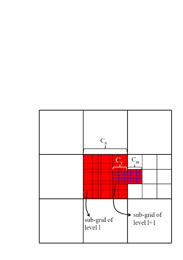
Figure 1: Sketch of the combination of AMR and DG sub-cell reconstruction. The cell $\mathcal{C}_{n}$ at level $\ell$ and the cell $\mathcal{C}_{m}$ at level $\ell+1$ (both in red) have limiter status $\beta=1$. The cell $\mathcal{C}_{n}$ must project $\textbf{v}_{h}$ from the sub-grid of level $\ell$ to the sub-grid of level $\ell+1$ in the virtual cell $\mathcal{C}_{v}$. (see color version on-line).

6 Numerical results

6.1 Euler equations of compressible gas dynamics

The first set of PDEs that we have considered in our numerical tests is represented by the classical Euler equations, which can be written as a system of conservation laws as required by Eq. (1), where the conserved variables and the corresponding fluxes are given by

$$\mathbf{u}=\left[\begin{array}[]{c}\rho\\ \rho\mathbf{v}\\ E\end{array}\right],~{}~{}~{}{\mathbf{F}}=\left[\begin{array}[]{c}\rho\mathbf{v}\\ \rho\mathbf{v}\mathbf{v}+p\mathbf{I}\\ (E+p)\mathbf{v}\end{array}\right].$$ (27)

Here $\mathbf{v}=(u,v,w)$ are the velocity components, $p$ is the pressure, $\rho$ is the mass density, $E=p/(\gamma-1)+\rho\mathbf{v}^{2}/2$ is the total energy density including the thermal and the kinetic contributions, $\mathbf{I}$ is the identity matrix, while $\gamma$ is the adiabatic index of the ideal gas, which follows the standard equation of state

$$p=\rho\epsilon(\gamma-1)\,,$$ (28)

where $\epsilon$ is the internal energy per unit mass. The Jacobian matrix associated to the Euler equations has eigenvalues that are all real and a set of linearly independent eigenvectors [117], thus allowing for the implementation of a large class of Riemann solvers. In the six subsections below we discuss a sample of classical test cases that involve the propagation of linear and non-linear waves admitted by the Euler equations. For practical purposes, we have represented in blue the unlimited cells, which, in the last time step, have been successfully evolved through the standard ADER-DG-AMR scheme. Conversely, we have represented in red the troubled cells, with limiter status $\beta=1$, which required the activation of the subcell limiter.

6.1.1 Numerical convergence study

In order to asses the convergence properties of the ADER-DG-AMR scheme we have considered the solution of the two-dimensional isentropic vortex, which admits an analytic solution [107]. The test consists of the advection of a vortex with initial conditions given by a perturbation superposed to a uniform mean flow as

$$\left(\rho,u,v,w,p\right)=(1+\delta\rho,1+\delta v_{x},1+\delta v_{y},0,1+\delta p)\,,$$ (29)

with

$$\left(\begin{array}[]{c}\delta\rho\\ \delta v_{x}\\ \delta v_{y}\\ \delta p\end{array}\right)=\left(\begin{array}[]{c}(1+\delta T)^{1/(\gamma-1)}-1\\ -(y-5)\epsilon/2\pi\exp{[0.5(1-r^{2})]}\\ \phantom{-}(x-5)\epsilon/2\pi\exp{[0.5(1-r^{2})]}\\ (1+\delta T)^{\gamma/(\gamma-1)}-1\end{array}\right).~{}~{}~{}$$ (30)

The perturbation in the temperature is

$$\delta T=-\frac{\epsilon^{2}(\gamma-1)}{8\gamma\pi^{2}}~{}\exp{(1-r^{2})}\,,$$ (31)

where $r^{2}=(x-5)^{2}+(y-5)^{2}$, while the vortex strength is $\epsilon=5$ and the adiabatic index is $\gamma=1.4$. It is easy to check that, under these conditions, the entropy per unit mass $s=p/\rho^{\gamma}$ is constant everywhere. The numerical domain is the square $\Omega=[0,10]\times[0,10]$, and periodic boundary conditions are used along the four edges. In this way, after setting the final time of the simulation to $t_{\rm final}=10$, the vortex recovers the initial position. We have solved this problem using the Rusanov flux with reconstruction in characteristic variables. Due to the smoothness of the solution, we expect that the sub-cell limiter is never activated, which is indeed the case. We have performed a convergence study by varying $N$ from 2 to 8, with $\ell_{\rm max}=1$ and a refinement factor $\mathfrak{r}=3$, except for the case $N=8$, for which we have used $\mathfrak{r}=2$. A regular refinement over the moving vortex is better obtained by applying a refinement criterion based on the cell average of the mass density, rather than by applying the standard procedure based on Eq. (22). In practice, and just for this test, a cell is marked for refinement if the cell average of the variable $\rho$ is smaller than the threshold $\bar{\rho}=0.75$. Table 1 summarizes the results of this analysis by reporting the $L^{1},L^{2}$ and $L^{\infty}$ norms of the error, computed with respect to the available analytic solution at time $t=t_{\rm final}$. The second column of the table reports the number of cells, along each direction, of the initial grid at the level zero. When $N\geq 6$, very coarse initial meshes have been adopted, since for larger values of $N_{x}$ the round-off errors affect negatively the outcome of the test. With this caveat in mind, the computed orders of convergence are in very good agreement with the nominal ones up to $N=8$, thus confirming the high order of accuracy of the proposed ADER-DG scheme even in combination with AMR and time-accurate local time stepping.

2D isentropic vortex problem — ADER-DG-$\mathbb{P}_{N}$ + WENO3 SCL
	$N_{x}$	$L^{1}$ error	$L^{2}$ error	$L^{\infty}$ error	$L^{1}$ order	$L^{2}$ order	$L^{\infty}$ order	Theor.
DG-$\mathbb{P}_{2}$	15	5.5416E-2	1.1075E-2	1.2671E-2	—	—	—	3
	30	5.7101E-3	1.0984E-3	1.7374E-3	3.28	3.33	2.87
	60	8.8511E-4	1.8805E-4	3.4727E-4	2.69	2.55	2.32
	90	3.0025E-4	6.6257E-5	1.3176E-4	2.67	2.57	2.39
DG-$\mathbb{P}_{3}$	15	6.4357E-3	1.0325E-3	1.0026E-3	—	—	—	4
	30	2.9981E-4	4.4304E-5	4.2822E-5	4.42	4.54	4.55
	60	1.1141E-5	1.6679E-6	2.2108E-6	4.75	4.73	4.27
	90	1.6787E-6	2.9117E-7	5.0366E-7	4.67	4.30	3.65
DG-$\mathbb{P}_{4}$	10	5.0587E-3	8.2103E-4	1.0921E-3	—	—	—	5
	15	6.3888E-4	1.0137E-4	1.2972E-4	5.10	5.16	5.25
	20	1.5369E-4	2.3219E-5	3.5064E-5	4.95	5.12	4.55
	25	5.1581E-5	7.8567E-6	1.2824E-5	4.89	4.86	4.51
DG-$\mathbb{P}_{5}$	15	1.1135E-4	1.6708E-5	2.5184E-5	—	—	—	6
	20	1.8700E-5	2.7597E-6	3.4678E-6	6.20	6.26	6.89
	25	3.9941E-6	6.0874E-7	9.4323E-7	6.92	6.77	5.83
	30	1.4623E-6	2.1969E-7	3.0234E-7	5.51	5.59	6.24
DG-$\mathbb{P}_{6}$	5	1.5485E-2	2.5835E-3	2.6686E-3	—	—	—	7
	10	1.8390E-4	2.9877E-5	4.1129E-5	6.40	6.43	6.02
	15	9.8578E-6	1.6642E-6	2.9090E-6	7.22	7.12	6.53
	20	1.2041E-6	2.0205E-7	3.6192E-7	7.31	7.33	7.24
DG-$\mathbb{P}_{7}$	5	6.2402E-3	1.0963E-3	1.4947E-3	—	—	—	8
	9	6.0168E-5	1.0210E-5	1.2830E-5	7.90	7.96	8.09
	11	1.5676E-5	2.4524E-6	4.0665E-6	6.70	7.11	5.73
	13	4.8297E-6	7.7831E-7	1.0593E-6	7.05	6.87	8.05
DG-$\mathbb{P}_{8}$	7	1.3473E-4	2.1259E-5	2.3665E-5	—	—	—	9
	9	1.8066E-5	2.8661E-6	3.6534E-6	7.99	7.97	7.43
	11	2.7718E-6	4.2166E-7	5.2952E-7	9.34	9.55	9.62
	13	6.2220E-7	1.0475E-7	1.4401E-7	8.94	8.34	7.79

Table 1: $L^{1},L^{2}$ and $L^{\infty}$ errors and convergence rates for the 2D isentropic vortex problem for the ADER-DG-$\mathbb{P}_{N}$ scheme with sub-cell limiter and adaptive mesh refinement. One level of refinement has been used with a refinement factor $\mathfrak{r}=3$, except for the case $N=8$, for which we have used $\mathfrak{r}=2$.

6.1.2 Riemann problems

Having verified the convergence properties of the ADER-DG-AMR scheme, we have considered two classical Riemann problems, proposed by Sod and Lax, with initial conditions given, respectively, by

$$(\rho,u,p)_{\rm Sod}=\left\{\begin{array}[]{llll}(1.0,0.0,1.0)&{\rm if}&x\in[0;0.5]\,,\\ (0.125,0.0,0.1)&{\rm if}&x\in[0.5;1.0]\,,\end{array}\right.$$ (32)

and

$$(\rho,v,p)_{\rm Lax}=\left\{\begin{array}[]{llll}(0.445,0.698,3.528)&{\rm if}&x\in[0;0.5]\,,\\ (0.5,0.0,0.571)&{\rm if}&x\in[0.5;1.0]\,.\end{array}\right.$$ (33)

The computational domain is actually two-dimensional, but the second direction $y$ acts as a passive one. Moreover, the adiabatic index of the gas is $\gamma=1.4$, and the final time of the simulation is $t_{\text{final}}=0.2$ for Sod’s problem, while it is $t_{\text{final}}=0.14$ for Lax’s. Both tests have been solved using the ADER-DG-$\mathbb{P}_{9}$ scheme, supplemented with our a posteriori ADER-WENO3 finite volume sub-cell limiter. The initial grid is composed of $N_{x}\times N_{y}=20\times 5$ cells, which are then adaptively refined using $\mathfrak{r}=3$ and $\ell_{\rm max}=2$. The results of our calculations, for which we have used the Osher flux [49], are reported in Figs. 2–3. Figure 2, in particular, shows the three-dimensional view of the solution by plotting the corresponding polynomials, highlighted in blue (for the unlimited cells) and in red (for the limited cells) according to our standard convention. We recall that the blue polynomials really represent the DG polynomials within each cell, while in the red cells we visualize the data as a piecewise linear interpolation of the subcell averages, produced by the subcell limiter. As in Fig. 4 of [53], in both the tests the contact discontinuity is resolved within one single cell, which, due to our AMR algorithm, in the present case is always at the maximum level of refinement. We further note that the contact wave is unlimited (blue). This is due to the fact that after a certain time our ADER-DG scheme recognizes this linear degenerate wave as a smooth feature, after the initial smoothing of the contact discontinuity by the subcell limiter and the Riemann solver. The right propagating shock, on the contrary, is always limited (red), as expected, and it is very sharply resolved. In Fig. 3 we have instead reported the comparison of the exact solution of the Riemann problem [117] with the numerical solution for a few representative variables, extracted from the polynomial data representation of the DG scheme -or the subcell limiter- along a 1D line of 200 equidistant sample points. The agreement between numerical and exact solution is excellent. Finally, for this test we have also performed a profiling analysis to quantify the relative computational costs of the subcell limiter. In a representative simulation using the ADER-DG-$\mathbb{P}_{2}$ scheme, with approximately $15\%$ of the cells that are limited, the overhead with respect to the unlimited DG scheme amounts to a factor $\approx 1.5$ in terms of CPU time.

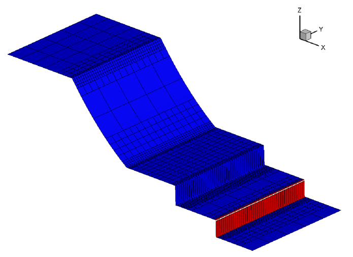
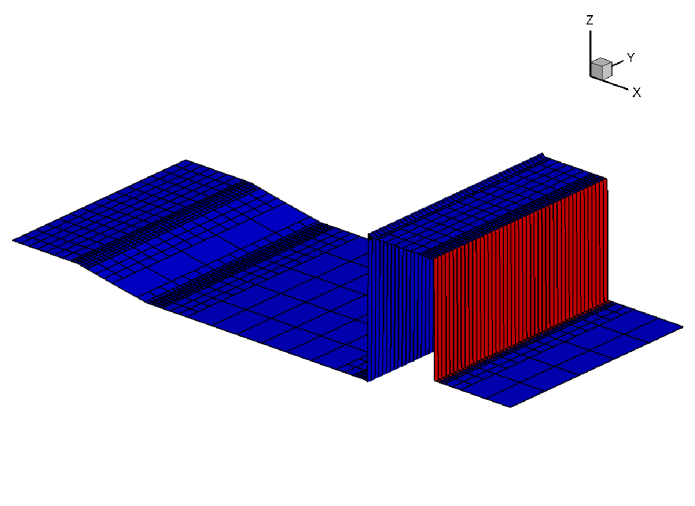
Figure 2: 3D view of the density variable and of the corresponding AMR grid. Top panel: Sod problem at $t_{\text{final}}=0.2$. Bottom panel: Lax problem at $t_{\text{final}}=0.14$. The limited cells, using the sub-cell ADER-WENO3 finite volume scheme, are highlighted in red, while unlimited DG-$\mathbb{P}_{9}$ cells are highlighted in blue.

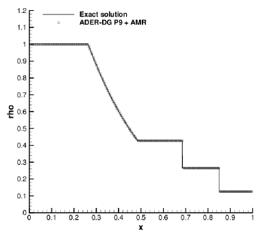
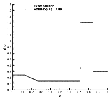
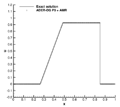
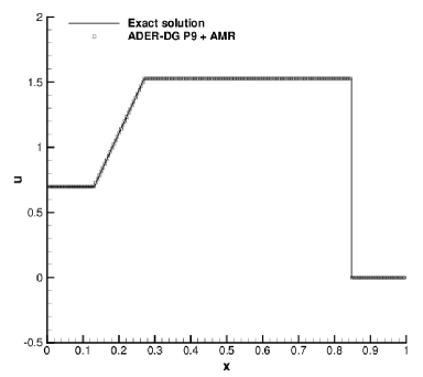
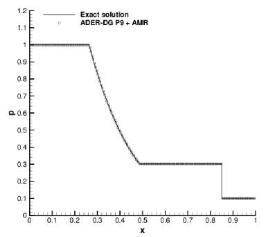
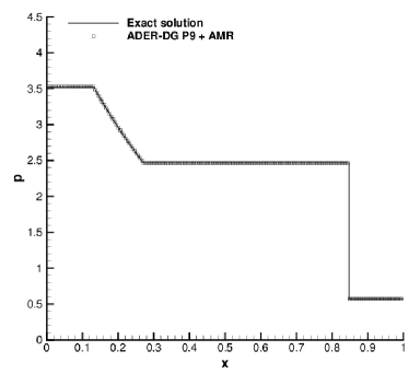
Figure 3: Sod shock tube problem (left panels) at $t_{\text{final}}=0.2$ and Lax problem (right panels) at $t_{\text{final}}=0.14$.

6.1.3 Double Mach reflection problem

A complex test problem in two space dimensions which contains a variety of waves such as strong shock waves, contact waves and shear waves, we have considered the so called double Mach reflection problem, which was first proposed in [124]. The initial conditions are given by a right-moving shock wave with a Mach number $M=10$, which intersects the $x-$ axis at $x=1/6$ with an inclination angle of $\alpha=60^{\circ}$. In order to provide the physical states ahead and behind the shock, it is necessary to solve the Rankine–Hugoniot conditions, which provide

$$(\rho,u,v,p)(\mathbf{x},t=0)=\left\{\begin{array}[]{cll}\frac{1}{\gamma}(8.0,8.25,0.0,116.5),&\text{ if }&\quad x^{\prime}<0.1,\\ (1.0,0.0,0.0,\frac{1}{\gamma}),&\text{ if }&\quad x^{\prime}\geq 0.1,\end{array}\right.$$ (36)

where $x^{\prime}=(x-1/6)\cos\alpha-y\sin\alpha$ is the coordinate in the rotated frame, while $\gamma=1.4$. The boundary conditions on the left side and on the right side are just given by inflow and outflow, while on the bottom we have used reflecting boundary conditions. On the other hand, the boundary conditions on the top require some more attention, since we need to impose the exact solution of an isolated moving oblique shock wave with the same shock Mach number $M_{s}=10$. The computational domain is given by $\Omega=[0;3.0]\times[0;1]$, which is covered by an initial uniform grid composed of $75\times 25$ cells. For our simulations, the Rusanov flux has been used and AMR is activated with $\ell_{\rm max}=2$ and $\mathfrak{r}=3$. The results of our calculations at time $t=0.2$ are reported in Figs. 4-6, for which we have used three different schemes: ADER-DG-$\mathbb{P}_{N}$ with $N=2,5,8$. In all these figures we have zoomed into the interaction zone with $1.8\leq x\leq 2.8$ in order to highlight the differences among the orders of accuracy. Moreover, the bottom right panel in each of these figures refers to a configuration with a finer initial grid, composed of $150\times 50$ cells. Fig. 4, in particular, shows the contour lines of the density. Fig. 5 shows the AMR grid and the troubled cells, highlighted in red, which required the activation of the limiter. Finally, Fig. 6 reports the Schlieren images of the density. There are a number of comments that can be made about these results. First, and mostly obvious, all DG schemes can detect the shock waves very well. On the other hand, by increasing the order of accuracy, the vortex-type flow structures manifest a larger and richer rolling-up, especially in the transition from ADER-DG-$\mathbb{P}_{2}$ to ADER-DG-$\mathbb{P}_{5}$. Secondly, the largest number of troubled cells, including false-positive troubled cells, is present for the lowest order scheme, i.e. the ADER-DG-$\mathbb{P}_{2}$, and it is concentrated along the shocks, while leaving the vortex-type flow structures unaffected. This is reassuring, since it indicates that higher order DG schemes have better subcell resolution capabilities. Last but not least we would like to note that the vortices generated by the rolling of the shear waves create sound waves, which travel through the computational domain. Although these simulations do not contain physical viscosity, and as such the vortex generation and rolling is only controlled by numerical viscosity, we can deduce from our numerical results that the novel scheme is able to resolve shock waves properly, as well as shear waves, vortex structures and sound waves.

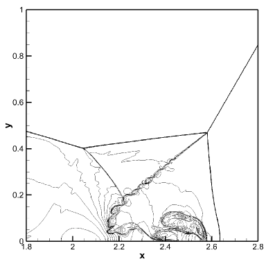
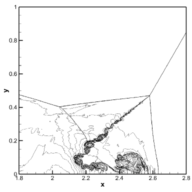
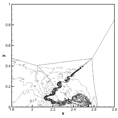
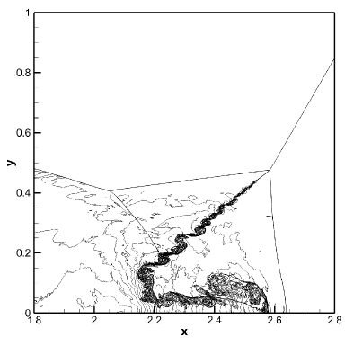
Figure 4: Zooms of the interaction zone for the double Mach reflection problem at $t=0.2$. Equidistant contour lines of the density variable are shown. Top left: AMR-ADER-DG-$\mathbb{P}_{2}$ with initial $75\times 25$ grid. Top right: AMR-ADER-DG-$\mathbb{P}_{5}$ with initial $75\times 25$ grid. Bottom left: AMR-ADER-DG-$\mathbb{P}_{8}$ with initial $75\times 25$ grid. Bottom right: AMR-ADER-DG-$\mathbb{P}_{5}$ with initial $150\times 50$ grid.

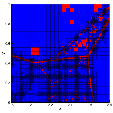
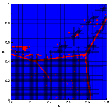
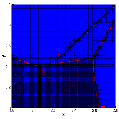
Figure 5: Zooms of the interaction zone for the double Mach reflection problem at $t=0.2$. The AMR grid and the limited cells (highlighted in red) are shown. Top left: ADER-DG-$\mathbb{P}_{2}$ with initial $75\times 25$ grid. Top right: ADER-DG-$\mathbb{P}_{5}$ with initial $75\times 25$ grid. Bottom left: ADER-DG-$\mathbb{P}_{8}$ with initial $75\times 25$ grid. Bottom right: ADER-DG-$\mathbb{P}_{5}$ with initial $150\times 50$ grid.

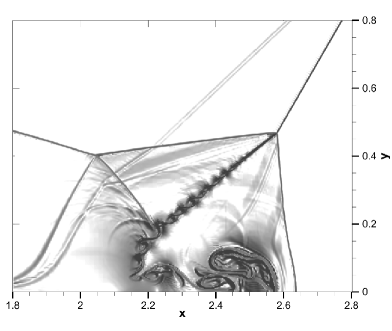
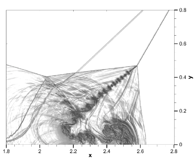
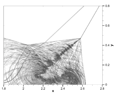
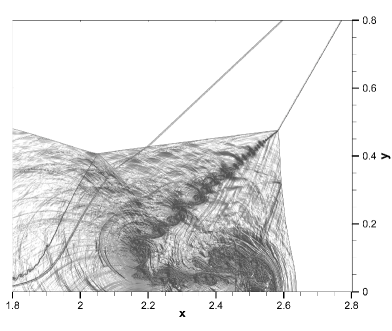
Figure 6: Schlieren image of the density variable for the double Mach reflection problem at $t=0.2$. Top left: ADER-DG-$\mathbb{P}_{2}$ with initial $75\times 25$ grid. Top right: ADER-DG-$\mathbb{P}_{5}$ with initial $75\times 25$ grid. Bottom left: ADER-DG-$\mathbb{P}_{8}$ with initial $75\times 25$ grid. Bottom right: ADER-DG-$\mathbb{P}_{5}$ with initial $150\times 50$ grid.

6.1.4 Forward facing step

The forward facing step problem is a classical test, often referred to as the Mach 3 wind tunnel test, which was proposed for the first time in [124]. We take as computational domain $\Omega=[0;3]\times[0;1]\backslash[0.6;3]\times[0;0.2]$. The initial conditions are given by a uniform flow moving to the right with Mach number $M=3$, $\rho=1$, $p=1/\gamma$, $u=3$, $v=0$, and adiabatic index $\gamma=1.4$. The final time of simulation is $t=4.0$. Regarding the boundary conditions, we have used reflecting boundaries at the lower and upper parts of the numerical domain, while inflow boundary conditions are imposed at the entrance and outflow boundary conditions at the exit. Figure 7 represents the numerical solution obtained using the ADER-DG-$\mathbb{P}_{5}$ scheme with a posteriori ADER-WENO3 sub-cell limiter. The panel on the top is a 2D view of the AMR grid showing, as usual, in red the limited cells and in blue the unlimited ones. The bottom panel, on the other hand, is a contour plot with 41 equidistant density contour levels in the interval $[0.1;4.5]$. The mesh at the coarsest level has $150\times 50$ cells, which is subsequently refined using AMR parameters $\ell_{\rm max}=2$ and $\mathfrak{r}=4$, corresponding to a uniform grid composed of $2400\times 800$ cells. It can be appreciated that there is a very good resolution of the physical instability and also it can be observed that both AMR and sub-cell limiter act where they are needed.

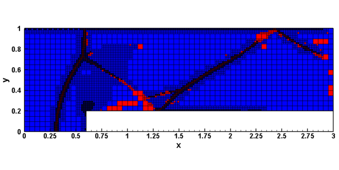
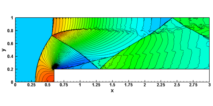
Figure 7: Forward facing step problem using ADER-DG-$\mathbb{P}_{5}$ with a posteriori ADER-WENO3 sub-cell limiter. Top: 2D view of the AMR grid together with limited cells (red) and unlimited cells (blue). Bottom: 41 equidistant density contour levels in the interval $[0.1;4.5]$.

6.1.5 2D Riemann problems

The two dimensional Riemann problems first proposed in [85] have become a classic benchmark for any numerical scheme solving the Euler equations. The initial conditions are represented by constant states in each of the four quadrants of the computational domain $\Omega=[-0.5;0.5]\times[-0.5;0.5]$, namely

$$\mathbf{u}(x,y,0)=\left\{\begin{array}[]{ccc}\mathbf{u}_{1}&\textnormal{ if }&x>0\wedge y>0,\\ \mathbf{u}_{2}&\textnormal{ if }&x\leq 0\wedge y>0,\\ \mathbf{u}_{3}&\textnormal{ if }&x\leq 0\wedge y\leq 0,\\ \mathbf{u}_{4}&\textnormal{ if }&x>0\wedge y\leq 0\,.\end{array}\right.$$ (37)

The data of the four configurations that we have considered are reported in Table 2. We emphasize that the adiabatic index is $\gamma=1.4$ in all cases.

Problem		$\rho$	$u$	$v$	$p$	$\rho$	$u$	$v$	$p$	$t_{\text{final}}$
		$x\leq 0$				$x>0$
RP1	$y>0$	0.5323	1.206	0.0	0.3	1.5	0.0	0.0	1.5	0.25
(Case 3 in KT)	$y\leq 0$	0.138	1.206	1.206	0.029	0.5323	0.0	1.206	0.3
RP2	$y>0$	0.5065	0.8939	0.0	0.35	1.1	0.0	0.0	1.1	0.25
(Case 4 in KT)	$y\leq 0$	1.1	0.8939	0.8939	1.1	0.5065	0.0	0.8939	0.35
RP3	$y>0$	2.0	0.75	0.5	1.0	1.0	0.75	-0.5	1.0	0.30
(Case 6 in KT)	$y\leq 0$	1.0	-0.75	0.5	1.0	3.0	-0.75	-0.5	1.0
RP4	$y>0$	1.0	0.7276	0.0	1.0	0.5313	0.0	0.0	0.4	0.25
(Case 12 in KT)	$y\leq 0$	0.8	0.0	0.0	1.0	1.0	0.0	0.7276	1.0

Table 2: Initial conditions for the two–dimensional Riemann problems. The ”Case No. in KT” refers to the classification of [85].

The simulations have been performed over a level zero grid of $50\times 50$ elements, adopting $\ell_{\rm max}=2$ and $\mathfrak{r}=3$. On the other hand, the numerical scheme is the ADER-DG-$\mathbb{P}_{5}$, with the Rusanov Riemann solver and reconstruction in characteristic variables. Fig. 8 shows the result of the simulations at the final time $t_{\text{final}}$ for each model. The left panels report the isolines of the density, while the right panels show, as usual, the AMR mesh and the cells updated through the sub-cell limiter, which have been highlighted in red. Due to the unprecedented high order of accuracy adopted, which reduces drastically the numerical dissipation of the numerical scheme, several small-scale features appear in the solution, typically attributed to the Kelvin–Helmholtz instability but not visible in the original versions shown by [85]. A similar effect was already noticed by [53] for the test RP3, even in the absence of AMR. However, when adaptive mesh refinement is activated, the effects of the Kelvin–Helmholtz instability emerge clearly also in model RP2 (along the diagonal of the cocoon structure), and in model RP4 (along the boundary of the bottom-left quadrant). Moreover, we emphasize that the use of AMR makes the sub-cell limiter operate only along strong discontinuities, which are resolved within very few cells at the maximum level of refinement.

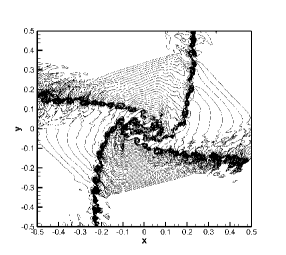
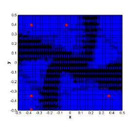
Figure 8: Two-dimensional Riemann problems solved with the AMR-ADER-DG-$\mathbb{P}_{5}$ method with sub-cell limiter on an initial uniform grid with $50\times 50$ cells. Two levels of refinement have been adopted, with refinement factor $\mathfrak{r}=3$. Left panels: isolines of the density. Right panels: AMR grid (black), limited cells (red) and unlimited cells (blue).

6.1.6 Cylindrical and spherical explosion problem

In multiple space dimensions, a conceptually simple but interesting extension of the one-dimensional Riemann problem is represented by the cylindrical and by the spherical explosion problem, both of them described with great detail in [115] and [117]. These two tests are indeed very relevant, since they involve the propagation of a shock wave that is not aligned with the coordinates, and they can therefore be used to check the ability of the numerical scheme in preserving the physical symmetries of the problem. As initial conditions, we assume the flow variables to be constant for $r\leq R$ and for $r\geq R$, namely

$$\big{(}\rho,u,v,w,p\big{)}=\left\{\begin{array}[]{ll}\big{(}1,0,0,0,1\big{)}&\;\textrm{for}\quad r\leq R\,,\\ \vskip 6.0pt plus 2.0pt minus 2.0pt\cr\big{(}0.125,0,0,0,0.1\big{)}&\;\textrm{for}\quad r>R\,,\end{array}\right.$$ (38)

where $r=\sqrt{\mathbf{x}^{2}}$ is the radial coordinate, $\mathbf{x}$ is the vector of spatial coordinates, while $R=0.5$ denotes the radius of the initial discontinuity. The computational domain is $\Omega=[-1;1]^{d}$, whereas the adiabatic index of the ideal-gas equation of state has been set to $\gamma=1.4$. As suggested by [117], a reference solution can be computed after solving an equivalent one dimensional problem in the radial direction $r$, in which the additional geometric terms arising from the choice of curvilinear coordinates can be moved to the right hand side of the governing PDEs as source terms.

We have solved the two-dimensional, cylindrical, explosion problem with the ADER-DG-$\mathbb{P}_{9}$ scheme in combination with our usual a posteriori sub-cell WENO finite volume limiter, the Osher-type flux of [49] and the reconstruction in characteristic variables. On the level zero grid, the mesh consists of $50\times 50$ elements, which are then refined using a refinement factor of $\mathfrak{r}=3$ and $\ell_{\max}=2$. This leads to an equivalent resolution on a uniform fine grid of $450\times 450=202,500$ elements. Considering that each P9 element uses 10 degrees of freedom per space dimension, this corresponds to a total resolution of $20,250,000$ spatial degrees of freedom on a uniform fine grid. Fig. 9 shows a 3D plot of the density distribution obtained for the cylindrical explosion case, as well as the AMR grid configuration at the final time $t=0.20$. Moreover, a 2D view of the AMR grid together with 1D cuts through the numerical solution on 150 equidistant sample points along the $x$-axis are depicted in Fig. 10. For comparison, Fig. 10 also contains the 1D reference solution as well as the numerical solution obtained with the ADER-DG-$\mathbb{P}_{9}$ scheme on the uniform fine grid. First of all, we observe that the numerical results coincide perfectly well with the reference solution. Secondly, one can note that the uniform fine grid solution as well as the result obtained with AMR are essentially identical.

In addition to the two dimensional case, we have also solved the spherical explosion problem in three spatial dimensions. In this case a very coarse initial mesh has been adopted, consisting of $13\times 13\times 13$ cells, which is subsequently refined using $\mathfrak{r}=3$ and $\ell_{\max}=2$. The problem has been solved with the ADER-DG-$\mathbb{P}_{3}$ scheme, Rusanov flux and reconstruction in characteristic variables. The results are shown in Fig. 11. As it is apparent from the top-left panel of this figure, the limiter has bee activated only at the shock front, at the contact discontinuity and at the head of the rarefaction wave. The comparison with the reference solution is also good.

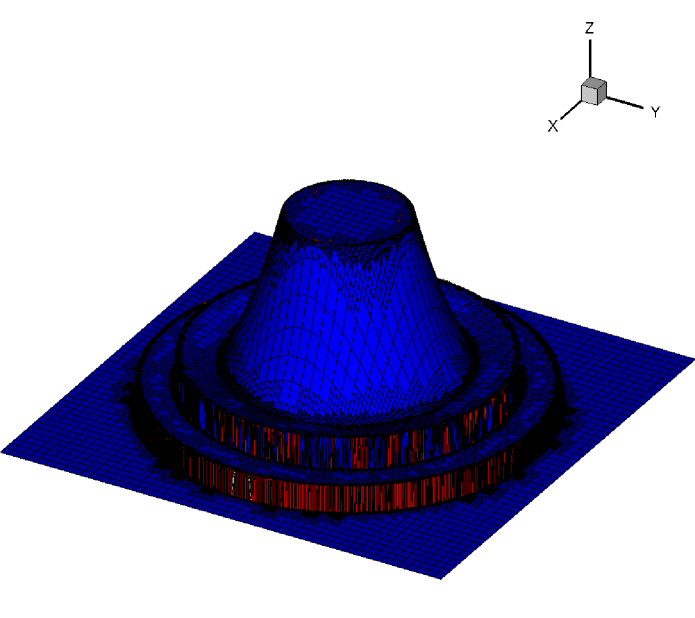
Figure 9: Three-dimensional view of the density variable and the AMR grid for the two dimensional explosion problem at $t_{\text{final}}=0.20$. Limited cells (red) updated with the sub-cell ADER-WENO3 finite volume scheme and unlimited cells (blue) with the ADER-DG-$\mathbb{P}_{9}$ scheme. The level zero AMR grid uses $50\times 50$ elements.

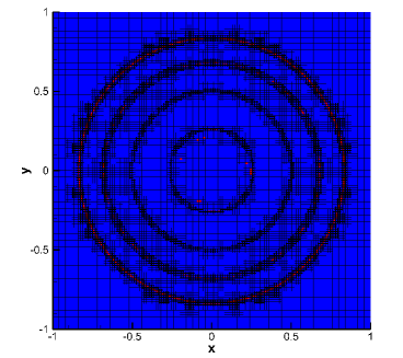
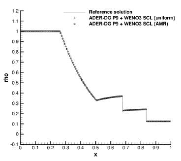
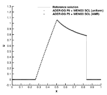
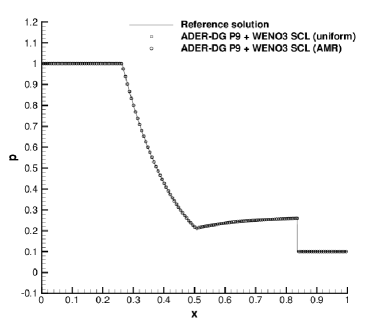
Figure 10: Two-dimensional explosion problem. 2D view of the AMR grid together with limited and unlimited cells (top left). One dimensional cuts of the numerical solution for density $\rho$ (top right), velocity $u$ (bottom left) and fluid pressure $p$ (bottom right) on 150 equidistant sample points along the positive $x-$axis obtained at $t_{\text{final}}=0.20$ with the space-time adaptive ADER-DG-$\mathbb{P}_{9}$ scheme, supplemented with a posteriori ADER-WENO3 sub-cell limiter. For comparison, the solution computed on a uniform fine mesh corresponding to the finest AMR grid level and the 1D reference solution are also reported.

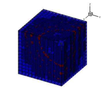
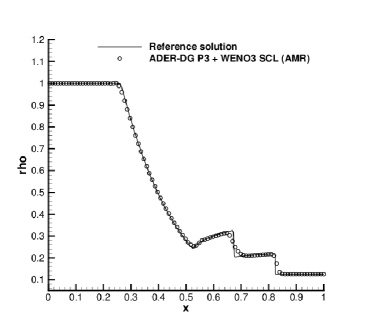
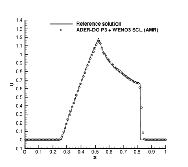
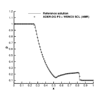
Figure 11: Three-dimensional explosion problem. 3D view of the AMR grid together with limited and unlimited cells (top left). One dimensional cuts of the numerical solution for density $\rho$ (top right), velocity $u$ (bottom left) and fluid pressure $p$ (bottom right) on 120 equidistant sample points along the positive $x-$axis obtained at $t_{\text{final}}=0.20$ with the space-time adaptive ADER-DG-$\mathbb{P}_{5}$ scheme, supplemented with a posteriori ADER-WENO3 sub-cell limiter.

6.2 Equations of ideal magnetohydrodynamics

A more complex and interesting hyperbolic system is represented by the classical equations of ideal magnetohydrodynamics (MHD). These equations are often used to model the dynamics of an electrically conducting fluid in which the hydrodynamic and the electromagnetic forces are comparable. Unlike the previous hyperbolic system for the classical Euler equations, an additional difficulty is that the numerical scheme must guarantee that the magnetic field $\mathbf{B}$ remains locally divergence-free, assuming that $\nabla\cdot\mathbf{B}=0$ at the initial time. While this is theoretically implied by the Maxwell equations, from the numerical point of view specific procedures must be adopted to prevent significant deviations from $\nabla\cdot\mathbf{B}=0$ due to accumulation of the numerical error. Over the years, several approaches have been adopted to solve this problem (see the review by [120]). In our work we have chosen the so-called divergence-cleaning procedure, which uses the hyperbolic version of the generalized Lagrangian multiplier (GLM) divergence cleaning method of [34]. By defining an additional auxiliary variable $\Phi$, a coupling term and a linear scalar PDE are introduced into the MHD system in order to allow the resulting augmented system to transport any possible divergence error (or numerical magnetic monopole) out of the numerical domain by itself, with an established cleaning velocity $c_{h}$. In this way, the augmented MHD system can be written in conservative form by defining the state vector $\mathbf{u}$ and the flux tensor $\mathbf{F}$ as

$$\mathbf{u}=\left[\begin{array}[]{c}\rho\\ \rho v_{j}\\ E\\ B_{j}\\ \Phi\end{array}\right],~{}~{}~{}{F^{i}}=\left[\begin{array}[]{c}\rho v_{i}\\ \rho v_{i}v_{j}+\left(p+\mathbf{B}^{2}/8\pi\right)\delta_{ij}-B_{i}B_{j}/4\pi\\ \left(E+p+\mathbf{B}^{2}/8\pi\right)v_{i}-\left(\mathbf{v}\cdot\mathbf{B}\right)B_{i}/4\pi\\ \epsilon_{jik}E_{k}+\Phi\delta_{ij}\\ c^{2}_{h}B_{i}\end{array}\right],\,\hskip 28.45274pti,j,k=x,y,z.$$ (39)

where $\mathbf{B}=(B_{x},B_{y},B_{z})$ is the magnetic field vector, $\mathbf{E}=(E_{x},E_{y},E_{z})$ is the electric field vector, $\delta_{ij}$ is the Kronecker delta and $\epsilon_{ijk}$ is the Levi-Civita symbol. The equation of state is again that of an ideal gas [cf. Eq. (28)], while the total energy density is given by $E=p/(\gamma-1)+\rho\mathbf{v}^{2}/2+\mathbf{B}^{2}/8\pi$. Moreover, for ideal MHD holds $\mathbf{E}=-\mathbf{v}\times\mathbf{B}$, so that in practice the electric field does not appear into the equations. In the following, we consider two nontrivial well-known problems of classical ideal MHD, by adopting the ADER-DG-$\mathbb{P}_{5}$ scheme, supplemented with our a posteriori WENO3 sub-cell limiter, with the Rusanov Riemann solver.

6.2.1 MHD rotor problem

Our first test is the MHD rotor problem sketched in [6]. The computational domain is $\Omega=[-0.6,0.6]\times[-0.6,0.6]$, with an initial mesh on the coarsest level composed of $50\times 50$ elements. The AMR framework is activated with $\mathfrak{r}=4$ and $\ell_{\text{max}}=2$. In this problem a high density fluid is rotating rapidly with angular velocity $\omega$, embedded in a low density fluid at rest. More specifically, the initial conditions are given by

$$\rho=\left\{\begin{array}[]{cl}10&\text{for}\;\;0\leq r\leq 0.1;\\ 1&\text{otherwise};\end{array}\right.,~{}~{}~{}\omega=\left\{\begin{array}[]{cl}10&\text{for}\;\;0\leq r\leq 0.1;\\ 0&\text{otherwise};\end{array}\right.,~{}~{}~{}{\mathbf{B}}=\left(\begin{array}[]{c}2.5\\ 0\\ 0\end{array}\right),~{}~{}~{}p=1\,.$$ (40)

Torsional Alfvén waves are generated by the spinning rotor and launched into the ambient medium. As a consequence, the angular momentum of the rotor is diminishing. In order to validate the accuracy of the method, the AMR computation is compared with the maximally refined uniform grid composed of $800\times 800=640,000$ elements, corresponding to a total resolution of $4800\times 4800=23,040,000$ spatial degrees of freedom on the uniform grid for the augmented MHD equations. Transmissive boundary conditions are applied at the borders. Following [6], a linear taper is applied in the range $0.1\leq r\leq 0.105$ to allow continuity of the physical variables between the internal rotor and the fluid at rest at $r=0.105$. The divergence cleaning velocity is set equal to $c_{h}=4$, while the adiabatic index is $\gamma=1.4$.

Figure 12 shows the solution for density, pressure, Mach number and magnetic pressure fields at time $t=0.25$. An excellent agreement between the AMR computation (reported in the left panels) and the uniform grid computation (reported in the right panels) is observed. Moreover, the numerical results are in very good agreement both with [6], and with the results of the ADER-WENO scheme with space-time adaptive mesh refinement presented in [52]. We would like to stress that spurious oscillations are absent in the density and the magnetic pressure fields, because of the adopted divergence cleaning procedure. In fact, without divergence cleaning, Godunov’s schemes would suffer of unphysical oscillations as reported by [6]. Finally, Fig. 13 shows the AMR mesh in the left panel and in the right panel the troubled zones in red, for which activation of the subcell limiter became necessary.

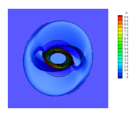
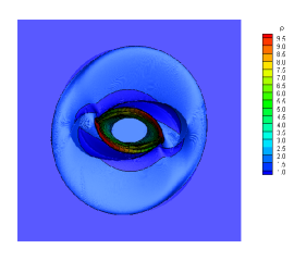
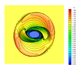
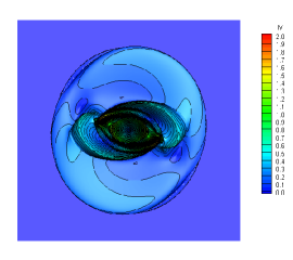
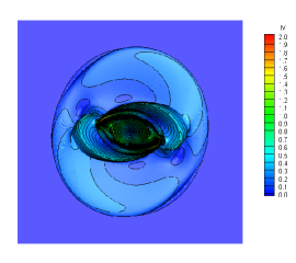
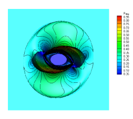
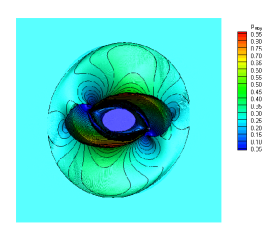
Figure 12: MHD rotor problem at time $t=0.25$ solved with ADER-DG-$\mathbb{P}_{5}$. Left panels: solution obtained on the AMR grid. Right panels: solution obtained on a fine uniform grid corresponding to the finest AMR grid level.

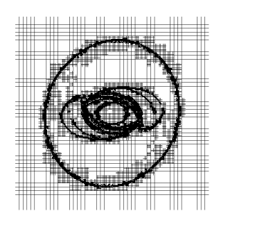
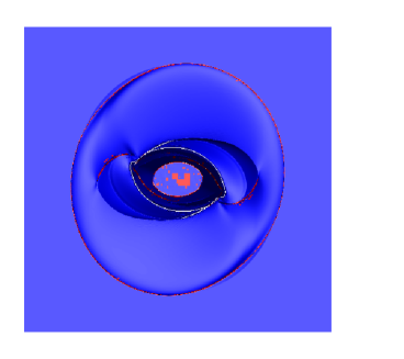
Figure 13: MHD rotor problem at time $t=0.25$: AMR grid on the left; troubled cells (red) and unlimited cells (blue) on the right.

6.2.2 Orszag-Tang vortex system

The second test that we have considered concerns the well known Orszag-Tang vortex problem, presented in [95], and later investigated by [99] and [33]. The adopted parameters refer to the computation performed by [76]. Because of the chosen normalization of the magnetic field, our initial conditions are

$$\left(\rho,u,v,w,p,B_{x},B_{y},B_{z}\right)=\left(\gamma^{2},-\sin\left(y\right),\sin\left(x\right),0,-\sqrt{4\pi}\sin\left(y\right),\sqrt{4\pi}\sin\left(2x\right),0\right),$$ (41)

where $\gamma=5/3$. The computational domain $\Omega=[0,2\pi]\times[0,2\pi]$ is discretized with $30\times 30$ elements on the coarsest refinement level at $t=0$. Periodic boundary conditions are applied along each edge. By using $\mathfrak{r}=3$ and $\ell_{\text{max}}=2$, the associated maximally refined uniform grid is formed of $270\times 270=72,000$ elements, that correspond to a total resolution of $2,624,400$ spatial degrees of freedom. The resulting solution for density, pressure, Mach number and magnetic pressure is plotted at times $t=0.5,2.0,3.0,5.0$ in Fig.14, both for the AMR and for the uniform grid. The AMR results appear to be in very good agreement with the reference solution represented by the calculation over the uniform grid. Moreover, our computations are in agreement with the the fifth order WENO finite difference results presented by [76], with the solution of [41] obtained with an unstructured third order WENO scheme, and also with the ADER-WENO solution computed with space-time adaptive mesh refinement in [52].

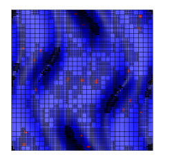
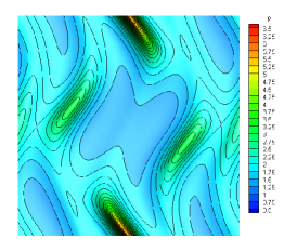
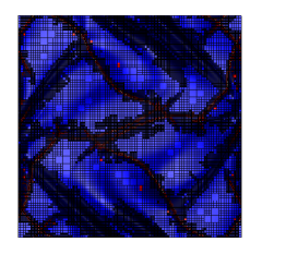
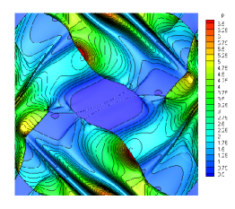
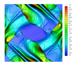
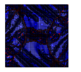
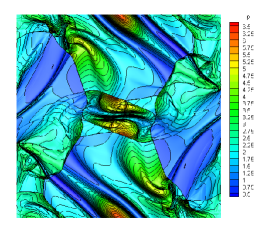
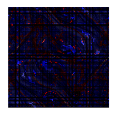
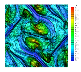
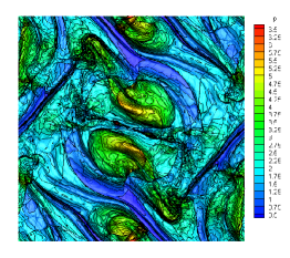
Figure 14: Orszag-Tang vortex problem at times $t=0.5$, $t=2.0$, $t=3.0$, $t=5.0$ (from top to bottom) obtained through the ADER-DG-$\mathbb{P}_{5}$ scheme supplemented with a posteriori ADER-WENO3 sub-cell limiter. Left panels: AMR-grid, troubled cells (red) and unlimited cells (blue). Central panels: $\mathbb{P}_{5}$-solution obtained on the AMR grid. Right panels: $\mathbb{P}_{5}$-solution obtained on the uniform grid corresponding to the finest AMR grid level.

7 Conclusion

In this paper we have extended the ADER-DG method with a posteriori ADER-WENO subcell finite volume limiters, which has been recently proposed in [53], to the context of space-time adaptive mesh refinement (AMR) in two and three space dimensions. The scheme itself is a modification of the pure discontinuous Galerkin (DG) finite element method that incorporates a novel idea for an a posteriori limiter. In practice, when a cell manifests significant oscillations, which is quite often the case for DG schemes in the presence of discontinuities, a sub-grid composed of $2N+1$ sub-cells is created and the corrupted solution is recomputed. This is done by recovering the solution at the previous time level, by projecting it onto the sub-cells to obtain an alternative data representation in terms of sub-cell averages, and, finally, by applying an ADER-WENO evolution in time, so as to completely replace the solution in the cell that was marked as troubled. The interlink with AMR requires a proper communication among the sub-grids at different levels of refinement. In particular, both projection and averaging, the two typical AMR operations among refinement levels, must be extended to the subcell averages that represent the solution on the sub-grids. The new scheme has been validated over a wide sample of test cases for the Euler and for the ideal magnetohydrodynamics equations, both in two and in three spatial dimensions. The nominal order of convergence has been verified up to polynomials of degree $N=8$. The combination of high order ADER-DG schemes, a posteriori sub-cell ADER-WENO finite volume limiters within a cell-by-cell AMR framework allows for an unprecedented numerical accuracy. In the case of the double Mach reflection problem as well as for the two-dimensional Riemann problems that we have considered in this paper, the new numerical approach revealed unexpected details in the dynamics of the fluid. Extending the scheme to equations with stiff source terms and true physical dissipative processes is one of the next goals, but even in its present form the method is likely to contribute significantly to those fields of computational fluid dynamics where high resolution and low numerical dissipation are needed. Given the unprecedented resolution capabilities shown in various test cases, we are convinced that the method presented in this paper belongs to a new generation of shock capturing schemes for computational fluid dynamics. Future work may concern the extension of the present space-time adaptive algorithm to high order semi-implicit DG schemes, following the ideas outlined in [42, 112, 111, 20, 21, 22, 24, 25, 45].

References

- [1] A.Burbeau, P.Sagaut, and C.H. Bruneau. A problem-independent limiter for high-order runge-kutta discontinuous galerkin methods. J. Comput. Phys., 169(1):111–150, May 2001.
- [2] G. Agbaglah, S. Delaux, D. Fuster, J. Hoepffner, C. Josserand, S. Popinet, P. Ray, R. Scardovelli, and S. Zaleski. Parallel simulation of multiphase flows using octree adaptivity and the volume-of-fluid method. Compte-rendus de l’Académie des Sciences, Paris, 339:194–207, 2011.
- [3] A. Baeza and P. Mulet. Adaptive mesh refinement techniques for high–order shock capturing schemes for multi–dimensional hydrodynamic simulations. International Journal for Numerical Methods in Fluids, 52:455–471, 2006.
- [4] D. Balsara, C. Altmann, C.D. Munz, and M. Dumbser. A sub-cell based indicator for troubled zones in RKDG schemes and a novel class of hybrid RKDG+HWENO schemes. Journal of Computational Physics, 226:586–620, 2007.
- [5] D. Balsara and C.W. Shu. Monotonicity preserving weighted essentially non-oscillatory schemes with increasingly high order of accuracy. Journal of Computational Physics, 160:405–452, 2000.
- [6] D. Balsara and D. Spicer. A staggered mesh algorithm using high order godunov fluxes to ensure solenoidal magnetic fields in magnetohydrodynamic simulations. Journal of Computational Physics, 149:270–292, 1999.
- [7] D.S. Balsara. Multidimensional HLLE Riemann solver: Application to Euler and magnetohydrodynamic flows. Journal of Computational Physics, 229:1970–1993, 2010.
- [8] D.S. Balsara. A two-dimensional HLLC Riemann solver for conservation laws: Application to Euler and magnetohydrodynamic flows. Journal of Computational Physics, 231:7476–7503, 2012.
- [9] D.S. Balsara. Multidimensional Riemann problem with self-similar internal structure. Part I – Application to hyperbolic conservation laws on structured meshes. Journal of Computational Physics, 277:163–200, 2014.
- [10] D.S. Balsara, M. Dumbser, and R. Abgrall. Multidimensional HLLC Riemann Solver for Unstructured Meshes - With Application to Euler and MHD Flows. Journal of Computational Physics, 261:172–208, 2014.
- [11] D.S. Balsara, C. Meyer, M. Dumbser, H. Du, and Z. Xu. Efficient implementation of ADER schemes for euler and magnetohydrodynamical flows on structured meshes – speed comparisons with runge–kutta methods. Journal of Computational Physics, 235:934 – 969, 2013.
- [12] C.E. Baumann and J.T. Oden. A discontinuous hp finite element method for the euler and navier-stokes equations. International Journal for Numerical Methods in Fluids, 31(1):79–95, 1999. cited By (since 1996)144.
- [13] C.E. Baumann and J. Tinsley Oden. A discontinuous hp finite element method for convection-diffusion problems. Computer Methods in Applied Mechanics and Engineering, 175(3-4):311–341, 1999. cited By (since 1996)221.
- [14] M. Ben-Artzi and J. Falcovitz. A second-order godunov-type scheme for compressible fluid dynamics. Journal of Computational Physics, 55:1–32, 1984.
- [15] M. J. Berger and P. Colella. Local adaptive mesh refinement for shock hydrodynamics. Journal of Computational Physics, 82:64–84, May 1989.
- [16] M. J. Berger and A. Jameson. Automatic adaptive grid refinement for the Euler equations. AIAA Journal, 23:561–568, 1985.
- [17] M. J. Berger and J. Oliger. Adaptive Mesh Refinement for Hyperbolic Partial Differential Equations. Journal of Computational Physics, 53:484, March 1984.
- [18] M.J. Berger, D.L. George, R.J. LeVeque, and L.T. Mandli. The geoclaw software for depth-averaged flows with adaptive refinement. Advances in Water Resources, 34(9):1195 – 1206, 2011. New Computational Methods and Software Tools.
- [19] A. Bourgeade, P. LeFloch, and P.A. Raviart. An asymptotic expansion for the solution of the generalized riemann problem. Part II: application to the gas dynamics equations. Annales de l’institut Henri Poincaré (C) Analyse non linéaire, 6:437–480, 1989.
- [20] L. Brugnano and V. Casulli. Iterative solution of piecewise linear systems. SIAM Journal on Scientific Computing, 30:463–472, 2007.
- [21] L. Brugnano and V. Casulli. Iterative solution of piecewise linear systems and applications to flows in porous media. SIAM Journal on Scientific Computing, 31:1858–1873, 2009.
- [22] L. Brugnano and A. Sestini. Iterative solution of piecewise linear systems for the numerical solution of obstacle problems. Journal of Numerical Analysis, Industrial and Applied Mathematics, 6:67–82, 2012.
- [23] C. C. Castro and E. F. Toro. Solvers for the high-order riemann problem for hyperbolic balance laws. Journal of Computational Physics, 227:2481–2513, 2008.
- [24] V. Casulli and P. Zanolli. A nested newton–type algorithm for finite volume methods solving richards’ equation in mixed form. SIAM Journal on Scientific Computing, 32:2255–2273, 2009.
- [25] V. Casulli and P. Zanolli. Iterative solutions of mildly nonlinear systems. Journal of Computational and Applied Mathematics, 236:3937–3947, 2012.
- [26] J. Cesenek, M. Feistauer, J. Horacek, V. Kucera, and J. Prokopova. Simulation of compressible viscous flow in time–dependent domains. Applied Mathematics and Computation, 219:7139–7150, 2013.
- [27] S. Clain, S. Diot, and R. Loubère. A high-order finite volume method for systems of conservation laws—multi-dimensional optimal order detection (MOOD). Journal of Computational Physics, 230(10):4028 – 4050, 2011.
- [28] B. Cockburn, S. Hou, and C. W. Shu. The Runge-Kutta local projection discontinuous Galerkin finite element method for conservation laws IV: the multidimensional case. Mathematics of Computation, 54:545–581, 1990.
- [29] B. Cockburn, S. Y. Lin, and C.W. Shu. TVB Runge-Kutta local projection discontinuous Galerkin finite element method for conservation laws III: one dimensional systems. Journal of Computational Physics, 84:90–113, 1989.
- [30] B. Cockburn and C. W. Shu. TVB Runge-Kutta local projection discontinuous Galerkin finite element method for conservation laws II: general framework. Mathematics of Computation, 52:411–435, 1989.
- [31] B. Cockburn and C. W. Shu. The Runge-Kutta local projection P1-Discontinuous Galerkin finite element method for scalar conservation laws. Mathematical Modelling and Numerical Analysis, 25:337–361, 1991.
- [32] B. Cockburn and C. W. Shu. The Runge-Kutta discontinuous Galerkin method for conservation laws V: multidimensional systems. Journal of Computational Physics, 141:199–224, 1998.
- [33] R. B. Dahlburg and J. M. Picone. Evolution of the orszag-tang vortex system in a compressible medium. I. initial average subsonic flow. Phys. Fluids B, 1:2153–2171, 1989.
- [34] A. Dedner, F. Kemm, D. Kröner, C.-D. Munz, T. Schnitzer, and M. Wesenberg. Hyperbolic divergence cleaning for the MHD equations. Journal of Computational Physics, 175:645–673, 2002.
- [35] S. Diot, S. Clain, and R. Loubère. Improved detection criteria for the multi-dimensional optimal order detection (MOOD) on unstructured meshes with very high-order polynomials. Computers and Fluids, 64:43 – 63, 2012.
- [36] S. Diot, R. Loubère, and S. Clain. The MOOD method in the three-dimensional case: Very-high-order finite volume method for hyperbolic systems. International Journal of Numerical Methods in Fluids, 73:362–392, 2013.
- [37] D.Kuzmin. Hierarchical slope limiting in explicit and implicit discontinuous galerkin methods. Journal of Computational Physics, 257, Part B(0):1140 – 1162, 2014. Physics-compatible numerical methods.
- [38] V. Dolejsi, M. Feistauer, and C. Schwab. On some aspects of the discontinuous galerkin finite element method for conservation laws. Mathematics and Computers in Simulation, 61(3-6):333–346, 2003.
- [39] R. Donat, M.C. Marti, A. MartÃnez-Gavara, and P. Mulet. Well-balanced adaptive mesh refinement for shallow water flows. Journal of Computational Physics, 257, Part A(0):937 – 953, 2014.
- [40] M. Dumbser. Arbitrary high order PNPM schemes on unstructured meshes for the compressible Navier–Stokes equations. Computers & Fluids, 39:60–76, 2010.
- [41] M. Dumbser, D. Balsara, E.F. Toro, and C.D. Munz. A unified framework for the construction of one-step finite-volume and discontinuous Galerkin schemes. Journal of Computational Physics, 227:8209–8253, 2008.
- [42] M. Dumbser and V. Casulli. A staggered semi-implicit spectral discontinuous galerkin scheme for the shallow water equations. Applied Mathematics and Computation, 219(15):8057–8077, 2013.
- [43] M. Dumbser, C. Enaux, and E.F. Toro. Finite volume schemes of very high order of accuracy for stiff hyperbolic balance laws. Journal of Computational Physics, 227:3971–4001, 2008.
- [44] M. Dumbser, A. Hidalgo, and O. Zanotti. High Order Space-Time Adaptive ADER-WENO Finite Volume Schemes for Non-Conservative Hyperbolic Systems. Computer Methods in Applied Mechanics and Engineering, 268:359–387, 2014.
- [45] M. Dumbser, U. Iben, and M. Ioriatti. An efficient semi-implicit finite volume method for axially symmetric compressible flows in compliant tubes. Applied Numerical Mathematics, 89:24–44, 2015.
- [46] M. Dumbser, M. Käser, and E. F. Toro. An Arbitrary High Order Discontinuous Galerkin Method for Elastic Waves on Unstructured Meshes V: Local Time Stepping and -Adaptivity. Geophysical Journal International, 171:695–717, 2007.
- [47] M. Dumbser and C.D. Munz. Building blocks for arbitrary high order discontinuous Galerkin schemes. Journal of Scientific Computing, 27:215–230, 2006.
- [48] M. Dumbser, T. Schwartzkopff, and C.D. Munz. Arbitrary high order finite volume schemes for linear wave propagation. In Computational Science and High Performance Computing II, Notes on Numerical Fluid Mechanics and Multidisciplinary Design (NNFM), pages 129–144. Springer, 2006.
- [49] M. Dumbser and E. F. Toro. On universal Osher–type schemes for general nonlinear hyperbolic conservation laws. Communications in Computational Physics, 10:635–671, 2011.
- [50] M. Dumbser, A. Uuriintsetseg, and O. Zanotti. On arbitrary-lagrangian-eulerian one-step weno schemes for stiff hyperbolic balance laws. Communications in Computational Physics, 14(2):301–327, 2013. cited By (since 1996)9.
- [51] M. Dumbser and O. Zanotti. Very high order PNPM schemes on unstructured meshes for the resistive relativistic MHD equations. Journal of Computational Physics, 228:6991–7006, 2009.
- [52] M. Dumbser, O. Zanotti, A. Hidalgo, and D.S. Balsara. ADER-WENO Finite Volume Schemes with Space-Time Adaptive Mesh Refinement. Journal of Computational Physics, 248:257–286, 2013.
- [53] M. Dumbser, O. Zanotti, R. Loubère, and S. Diot. A posteriori subcell limiting of the discontinuous Galerkin finite element method for hyperbolic conservation laws. Journal of Computational Physics, 278:47–75, December 2014.
- [54] S. Fechter and C.D. Munz. A discontinuous Galerkin based sharp-interface method to simulate three-dimensional compressible two-phase flow. International Journal for Numerical Methods in Fluids, 2015. DOI: 10.1002/fld.4022.
- [55] M. Feistauer, V. Dolejsi, and V. Kucera. On the discontinuous galerkin method for the simulation of compressible flow with wide range of mach numbers. Computing and Visualization in Science, 10(1):17–27, 2007.
- [56] M. Feistauer, V. Kucera, and J. Prokopová. Discontinuous galerkin solution of compressible flow in time–dependent domains. Mathematics and Computers in Simulation, 80(8):1612–1623, 2010.
- [57] P. Le Floch and P.A. Raviart. An asymptotic expansion for the solution of the generalized riemann problem. Part I: General theory. Annales de l’institut Henri Poincaré (C) Analyse non linéaire, 5:179–207, 1988.
- [58] G. Gassner, M. Dumbser, F. Hindenlang, and C.D. Munz. Explicit one–step time discretizations for discontinuous Galerkin and finite volume schemes based on local predictors. Journal of Computational Physics, 230:4232–4247, 2011.
- [59] G. Gassner and D.A. Kopriva. A comparison of the dispersion and dissipation errors of Gauss and Gauss-Lobatto discontinuous Galerkin spectral element methods. SIAM Journal on Scientific Computing, 33(5):2560–2579, 2011.
- [60] G. Gassner, F. Lörcher, and C. D. Munz. A discontinuous Galerkin scheme based on a space-time expansion II. viscous flow equations in multi dimensions. Journal of Scientific Computing, 34:260–286, 2008.
- [61] Emmanuil H. Georgoulis, Edward Hall, and Paul Houston. Discontinuous galerkin methods on hp-anisotropic meshes ii: a posteriori error analysis and adaptivity. Applied Numerical Mathematics, 59(9):2179 – 2194, 2009. Second Chilean Workshop on Numerical Analysis of Partial Differential Equations (WONAPDE 2007).
- [62] S.K. Godunov. Finite difference methods for the computation of discontinuous solutions of the equations of fluid dynamics. Mathematics of the USSR - Sbornik, 47:271–306, 1959.
- [63] C. R. Goetz and A. Iske. Approximate solutions of generalized Riemann problems for nonlinear systems of hyperbolic conservation laws. Mathematics of Computation. DOI: 10.1090/mcom/2970.
- [64] S. Gottlieb and C.W. Shu. Total variation diminishing Runge-Kutta schemes. Mathematics of Computation, 67:73–85, 1998.
- [65] A. Harten, B. Engquist, S. Osher, and S. Chakravarthy. Uniformly high order essentially non-oscillatory schemes, III. Journal of Computational Physics, 71:231–303, 1987.
- [66] R. Hartmann and P. Houston. Adaptive Discontinuous Galerkin Finite Element Methods for the Compressible Euler Equations. Journal of Computational Physics, 183:508–532, December 2002.
- [67] A. Hidalgo and M. Dumbser. ADER schemes for nonlinear systems of stiff advection-diffusion-reaction equations. Journal of Scientific Computing, 48:173–189, 2011.
- [68] H.Luo, J.D.Baum, and R.Löhner. A hermite weno-based limiter for discontinuous galerkin method on unstructured grids. J. Comput. Phys., 225(1):686–713, July 2007.
- [69] P. Houston, C. Schwab, and E. Süli. Stabilized hp-finite element methods for first-order hyperbolic problems. SIAM Journal on Numerical Analysis, 37(5):1618–1643, 2000. cited By (since 1996)50.
- [70] P. Houston, C. Schwab, and E. Súli. Discontinuous hp-finite element methods for advection-diffusion-reaction problems *. SIAM Journal on Numerical Analysis, 39(6):2133–2163, 2002. cited By (since 1996)190.
- [71] P. Houston and E. Süli. hp-adaptive discontinuous galerkin finite element methods for first-order hyperbolic problems. SIAM Journal on Scientific Computing, 23(4):1226–1252, 2002. cited By (since 1996)40.
- [72] L. Ivan and C.P.T. Groth. High-order central eno finite-volume scheme with adaptive mesh refinement for the advection-diffusion equation. Computational Fluid Dynamics 2008, pages 443 – 449, 2009.
- [73] L. Ivan and C.P.T. Groth. High-order solution-adaptive central essentially non-oscillatory (ceno) method for viscous flows. Journal of Computational Physics, 257, Part A(0):830 – 862, 2014.
- [74] G. Jiang and C.W. Shu. On a cell entropy inequality for discontinuous Galerkin methods. Mathematics of Computation, 62:531–538, 1994.
- [75] G.-S. Jiang and C.W. Shu. Efficient implementation of weighted ENO schemes. Journal of Computational Physics, 126:202–228, 1996.
- [76] G.S. Jiang and C.C. Wu. A high-order WENO finite difference scheme for the equations of ideal magnetohydrodynamics. Journal of Computational Physics, 150:561–594, 1999.
- [77] J.Qiu and C.W. Shu. Hermite WENO Schemes and Their Application As Limiters for Runge-Kutta Discontinuous Galerkin Method: One-dimensional Case. J. Comput. Phys., 193(1):115–135, January 2004.
- [78] J.Zhu, J. Qiu, C.W.Shu, and M.Dumbser. Runge-Kutta Discontinuous Galerkin Method Using WENO Limiters II: Unstructured Meshes. J. Comput. Phys., 227(9):4330–4353, April 2008.
- [79] C.W. Shu J.Zhu, X.Zhong and J. Qiu. Runge–kutta discontinuous galerkin method using a new type of weno limiters on unstructured meshes. J. Comp. Phys., 248:200–220, 2013.
- [80] A.M Khokhlov. Fully threaded tree algorithms for adaptive refinement fluid dynamics simulations. Journal of Computational Physics, 143(2):519 – 543, 1998.
- [81] M. A. Kopera and F. X. Giraldo. Analysis of adaptive mesh refinement for IMEX discontinuous Galerkin solutions of the compressible Euler equations with application to atmospheric simulations. Journal of Computational Physics, 275:92–117, October 2014.
- [82] D.A. Kopriva. Metric identities and the discontinuous spectral element method on curvilinear meshes. Journal of Scientific Computing, 26(3):301–327, 2006.
- [83] D.A. Kopriva and G. Gassner. On the quadrature and weak form choices in collocation type discontinuous galerkin spectral element methods. Journal of Scientific Computing, 44(2):136–155, 2010.
- [84] L. Krivodonova and R.Qin. An analysis of the spectrum of the discontinuous galerkin method. Applied Numerical Mathematics, 64:1–18, 2013.
- [85] A. Kurganov and E. Tadmor. Solution of two-dimensional Riemann problems for gas dynamics without Riemann problem solvers. Numer. Methods Partial Differential Equations, 18:584–608, 2002.
- [86] T. Leicht and R. Hartmann. Anisotropic mesh refinement for discontinuous galerkin methods in two-dimensional aerodynamic flow simulations. International Journal for Numerical Methods in Fluids, 56(11):2111–2138, 2008.
- [87] Y. Liu, M. Vinokur, and Z.J. Wang. Spectral (Finite) Volume Method for Conservation Laws on Unstructured Grids V: Extension to Three-Dimensional Systems. Journal of Computational Physics, 212:454–472, 2006.
- [88] L.Krivodonova. Limiters for high-order discontinuous Galerkin methods. Journal of Computational Physics, 226:879–896, September 2007.
- [89] R. Löhner. An adaptive finite element scheme for transient problems in {CFD}. Computer Methods in Applied Mechanics and Engineering, 61(3):323 – 338, 1987.
- [90] F. Lörcher, G. Gassner, and C. D. Munz. A discontinuous Galerkin scheme based on a space-time expansion. I. inviscid compressible flow in one space dimension. Journal of Scientific Computing, 32:175–199, 2007.
- [91] R. Loubère, M. Dumbser, and S. Diot. A new family of high order unstructured mood and ader finite volume schemes for multidimensional systems of hyperbolic conservation laws. Communication in Computational Physics, 16:718–763, 2014.
- [92] H. Lu and Q. Sun. A straightforward hp-adaptivity strategy for shock-capturing with high-order discontinuous galerkin methods. Advances in Applied Mathematics and Mechanics, 6(1):135–144, 2014. cited By (since 1996)0.
- [93] H. Luo, J.D. Baum, and R. Löhner. A discontinuous galerkin method based on a taylor basis for the compressible flows on arbitrary grids. Journal of Computational Physics, 227:8875–8893, 2008.
- [94] G. Montecinos, C.E. Castro, M. Dumbser, and E.F. Toro. Comparison of solvers for the generalized riemann problem for hyperbolic systems with source terms. Journal of Computational Physics, 231(19):6472–6494, 2012.
- [95] S. A. Orszag and C. M. Tang. Small-scale structure of two-dimensional magnetohydrodynamic turbulence. Journal of Fluid Mechanics, 90:129, 1979.
- [96] L. Pareschi and G. Russo. Implicit–explicit runge–kutta schemes and applications to hyperbolic systems with relaxation. Journal of Scientific Computing, 25(1):129, 2005.
- [97] L. Pareschi and G. Russo. Implicit-explicit runge-kutta schemes and applications to hyperbolic systems with relaxation. Journal of Scientific Computing, 25:129–155, 2005. 10.1007/s10915-004-4636-4.
- [98] P.-O. Persson and J. Peraire. Sub-cell shock capturing for discontinuous galerkin methods. AIAA Paper 2006-112, 2006.
- [99] J. M. Picone and R. B. Dahlburg. Evolution of the orszag-tang vortex system in a compressible medium. II. supersonic flow. Phys. Fluids B, 3:29–44, 1991.
- [100] J. Qiu, M. Dumbser, and C.W. Shu. The discontinuous Galerkin method with Lax-Wendroff type time discretizations. Computer Methods in Applied Mechanics and Engineering, 194:4528–4543, 2005.
- [101] J. Qiu and C.W. Shu. Hermite WENO schemes and their application as limiters for Runge-Kutta discontinuous Galerkin method II: two dimensional case. Computers and Fluids, 34:642–663, 2005.
- [102] J. Qiu and C.W. Shu. Runge-Kutta discontinuous Galerkin method using WENO limiters. SIAM Journal on Scientific Computing, 26:907–929, 2005.
- [103] D. Radice and L. Rezzolla. Discontinuous Galerkin methods for general-relativistic hydrodynamics: Formulation and application to spherically symmetric spacetimes. Phys. Rev. D, 84(2):024010, July 2011.
- [104] R.Biswas, K. D. Devine, and J. E. Flaherty. Parallel, adaptive finite element methods for conservation laws. APPL. NUMER. MATH, 14:255–283, 1994.
- [105] W.H. Reed and T.R. Hill. Triangular mesh methods for neutron transport equation. Technical Report LA-UR-73-479, Los Alamos Scientific Laboratory, 1973.
- [106] V. V. Rusanov. Calculation of Interaction of Non–Steady Shock Waves with Obstacles. J. Comput. Math. Phys. USSR, 1:267–279, 1961.
- [107] C.W. Shu. Essentially non-oscillatory and weighted essentially non-oscillatory schemes for hyperbolic Conservation Laws. NASA/CR-97-206253 ICASE Report No.97-65, November 1997.
- [108] M. Sonntag and C.D. Munz. Shock capturing for discontinuous galerkin methods using finite volume subcells. In J. Fuhrmann, M. Ohlberger, and C. Rohde, editors, Finite Volumes for Complex Applications VII, pages 945–953. Springer, 2014.
- [109] A.H. Stroud. Approximate Calculation of Multiple Integrals. Prentice-Hall Inc., Englewood Cliffs, New Jersey, 1971.
- [110] A. Taube, M. Dumbser, D. Balsara, and C.D. Munz. Arbitrary high order discontinuous Galerkin schemes for the magnetohydrodynamic equations. Journal of Scientific Computing, 30:441–464, 2007.
- [111] M. Tavelli and M. Dumbser. A high order semi-implicit discontinuous galerkin method for the two dimensional shallow water equations on staggered unstructured meshes. Applied Mathematics and Computation, 234:623–644, 2014.
- [112] M. Tavelli and M. Dumbser. A staggered arbitrary high order semi-implicit discontinuous galerkin method for the two dimensional incompressible navier-stokes equations. Applied Mathematics and Computation, 248:70–92, 2014.
- [113] V.A. Titarev and E.F. Toro. ADER: Arbitrary high order Godunov approach. Journal of Scientific Computing, 17(1-4):609–618, December 2002.
- [114] V.A. Titarev and E.F. Toro. Finite-volume weno schemes for three-dimensional conservation laws. Journal of Computational Physics, 201:238–260, 2004.
- [115] V.A. Titarev and E.F. Toro. ADER schemes for three-dimensional nonlinear hyperbolic systems. Journal of Computational Physics, 204:715–736, 2005.
- [116] E. F. Toro and V. A. Titarev. Derivative Riemann solvers for systems of conservation laws and ADER methods. Journal of Computational Physics, 212(1):150–165, 2006.
- [117] E.F. Toro. Riemann Solvers and Numerical Methods for Fluid Dynamics. Springer, second edition, 1999.
- [118] E.F. Toro, R.C. Millington, and L.A.M Nejad. Towards very high order Godunov schemes. In E.F. Toro, editor, Godunov Methods. Theory and Applications, pages 905–938. Kluwer/Plenum Academic Publishers, 2001.
- [119] E.F. Toro and V. A. Titarev. Solution of the generalized Riemann problem for advection-reaction equations. Proc. Roy. Soc. London, pages 271–281, 2002.
- [120] Gabor Toth. The constraint in shock-capturing magnetohydrodynamics codes. Journal of Computational Physics, 161(2):605 – 652, 2000.
- [121] C.-C. Tsai, T.-H. Hou, S. Popinet, and Y. Y. Chao. Wind wave prediction of tropical cyclones by a quadtree-adaptive model. Coastal Engineering, pages 108–119, 2013.
- [122] Z.J. Wang and Y. Liu. Extension of the spectral volume method to high-order boundary representation. Journal of Computational Physics, 211:154–178, 2006.
- [123] Z.J. Wang, L. Zhang, and Y. Liu. Spectral (finite) volume method for conservation laws on unstructured grids iv: Extension to two-dimensional euler equations. Journal of Computational Physics, 194:716–741, 2004.
- [124] P. Woodward and P. Colella. The numerical simulation of two-dimensional fluid flow with strong shocks. Journal of Computational Physics, 54:115–173, 1984.
- [125] M. Yang and Z. Wang. A Parameter-Free Generalized Moment Limiter for High-Order Methods on Unstructured Grids. Advances in Applied Mathematics and Mechanics, 2009.
- [126] Y. Yu, D. Wu, and Y. Xu. Three dimensional discontinuous galerkin methods for euler equations on adaptive conforming meshes. Computer Physics Communications, 182(9):1771 – 1775, 2011.
- [127] O. Zanotti and M. Dumbser. Numerical simulations of high Lundquist number relativistic magnetic reconnection. Mon. Not. R. Astron. Soc., 418:1004–1011, December 2011.
- [128] O. Zanotti and M. Dumbser. A high order special relativistic hydrodynamic and magnetohydrodynamic code with space-time adaptive mesh refinement. Computer Physics Communications, 188:110–127, 2015.