Time-resolved spectroscopy in time dependent density functional theory: An exact condition

Abstract

A fundamental property of a quantum system driven by an external field is that when the field is turned off the positions of its response frequencies are independent of the time at which the field is turned off. We show that this leads to an exact condition for the exchange-correlation potential of time-dependent density functional theory. The Kohn-Sham potential typically continues to evolve after the field is turned off, which leads to time-dependence in the response frequencies of the Kohn-Sham response function. The exchange-correlation kernel must cancel out this time-dependence. The condition is typically violated by approximations currently in use, as we demonstrate by several examples, which has severe consequences for their predictions of time-resolved spectroscopy.

Time-resolved spectroscopies are increasingly being used to characterize and analyze processes in molecules and solids. Applying an ultrafast pump pulse to create a non-stationary state, which is then monitored in time by a probe pulse is a central technique in the field of femtochemistry Zewail (2000), and has revolutionized our understanding of chemical reactions and photo-induced processes in a wide range of systems including biological molecules and nanoscale devices. Until recently, experiments primarily probed ionic dynamics where time-resolved spectra reflect changes in the ionic configuration during a reaction Pollard and Mathies (1992). The recent advent of attosecond pulses enables pump-probe experiments at the time-scale of electron dynamics Krausz and Ivanov (2009), allowing investigations of processes on the electronic time-scale, and revealing a wealth of new phenomena and new possibilities for characterizing a system.

A scalable theoretical method to model electron dynamics, reliable beyond the perturbative regime, is crucial to simulate and interpret experimental results, and to suggest new experiments and materials to study. Time-dependent density functional theory (TDDFT), an exact reformulation of many-electron quantum mechanics, stands out with its balance between accuracy and computational cost Runge and Gross (1984); Marques et al. (2012a); Ullrich (2011). Non-interacting electrons evolve in a one-body potential such that the exact one-body density $n({\bf r},t)$ of the true system is reproduced. However in practice the exchange-correlation (xc) contribution to the potential must be approximated as a functional of the density and the initial interacting and Kohn-Sham (KS) states, $\Psi_{0},\Phi_{0}$ respectively: $v_{\scriptscriptstyle\rm XC}[n;\Psi_{0},\Phi_{0}](t)$. Most TDDFT calculations nowadays use adiabatic functionals, which depend exclusively on the instantaneous density, input into a ground-state functional: $v_{\scriptscriptstyle\rm XC}^{A}[n;\Psi_{0},\Phi_{0}](t)=v_{\scriptscriptstyle\rm XC}^{\rm g.s.}[n(t)]$.

TDDFT has been extensively and successfully applied to model the linear response of large systems and to elucidate experiments in the non-perturbative regime, e.g. Refs. Shinohara et al. (2012); Rozzi et al. (2013); Penka Fowe and Bandrauk (2011); Olof Johansson et al. (2013), including coherent phonon generation, strong-field and thermal ionization, harmonic generation, and exploring photovoltaic materials, to name a few. At the same time, however, recent work on small systems where numerically-exact or high-level wavefunction methods are applicable, has shown that the approximate TDDFT functionals can yield significant errors in their predictions of the dynamics Elliott et al. (2012); Luo et al. (2014); Thiele et al. (2008); Ramsden and Godby (2012); Ruggenthaler and Bauer (2009); Fuks et al. (2013, 2011); Raghunathan and Nest (2011); Habenicht et al. (2014); Ramakrishnan and Nest (2012); Raghunathan and Nest (2012), and sometimes they fail even qualitatively Fuks et al. (2013, 2011); Ruggenthaler and Bauer (2009); Raghunathan and Nest (2011); Ramakrishnan and Nest (2012); Raghunathan and Nest (2012); Habenicht et al. (2014).

A critical aspect of non-equilibrium dynamics are the response frequencies of the system, since these play a crucial role in the response to an applied field, and in interferences in the dynamics. As pointed out recently, approximate functionals yield erroneous time-dependent electronic structure when subject to external fields Ramakrishnan and Nest (2012); Raghunathan and Nest (2012); De Giovannini et al. (2013). This spurious “peak shifting” makes TDDFT simulations of resonant coherent control very challenging Ramakrishnan and Nest (2012), and the interpretation of time-resolved spectroscopic simulations difficult.

Let a “pumped system” refer to a system which has been driven out of its ground-state by an external field for time $\mathcal{T}$, after which the field is turned off. In this paper we derive an exact condition that the xc functional must satisfy in order to respect a fundamental property of the response frequencies of the pumped system: For times $\mathcal{T}$ short enough that ionic motion can be neglected, its response frequencies are independent of $\mathcal{T}$. The oscillator strengths may change in strength and sign but the response frequencies remain constant. We define the response frequencies via poles in the density-density linear response function evaluated about an arbitrary state in the absence of any externally applied fields. Most TDDFT functionals currently in use violate this condition, with severe implications for the modeling of time-resolved spectroscopy. Several model examples are given to illustrate the impact of the violation on dynamics, including examples of an adiabatic functional that, despite inaccurate response frequencies, approximately satisfies this condition, and consequently yields accurate dynamics.

After the field is turned off at time $\mathcal{T}$, then, treating the nuclei as stationary, the Hamiltonian is static, $\hat{H}^{(0)}=\hat{T}+\hat{W}+\hat{v}_{\rm ext}^{(0)}$, the sum of the kinetic energy, electron-interaction, and electron-nuclear interaction operators respectively. The electronic state can be expanded in terms of the eigenstates $\Psi_{n}$: $\Psi(t\geq\mathcal{T})=\sum_{n}c_{n}(\mathcal{T})\Psi_{n}e^{-iE_{n}(t-\mathcal{T})}$, with $\hat{H}^{(0)}\Psi_{n}=E_{n}\Psi_{n}$. We denote the density of this state as $n^{(0)}_{\mathcal{T}}({\bf r},t)$, defined for times $t\geq\mathcal{T}$. Throughout the paper, the superscript ${(0)}$ indicates a quantity in the absence of external fields. We define a non-equilibrium response function to describe the density response to a perturbation $\delta v_{\rm ext}({\bf r},t)$ (probe) applied after time $\mathcal{T}$:

$$\tilde{\chi}[n^{(0)}_{\mathcal{T}};\Psi(\mathcal{T})]({\bf r},{\bf r}^{\prime},t,t^{\prime})=\left.\frac{\delta n({\bf r},t)}{\delta v_{\rm ext}({\bf r}^{\prime},t^{\prime})}\right|_{n^{(0)}_{\mathcal{T}},\Psi(\mathcal{T})}\;\;.$$ (1)

Here the functional dependences on the left-hand-side follow from the Runge-Gross theorem Runge and Gross (1984), considering the onset of the free-evolution ($t=\mathcal{T}$) as the initial time. (Note that Eq.(1) applies for the response of any arbitrary state $\Psi(\mathcal{T})$, not just those reached by a pump field). Following derivations in standard linear response theory Giuliani and Vignale (2005) but generalized to an arbitrary initial state, $\tilde{\chi}[n^{(0)}_{\mathcal{T}};\Psi(\mathcal{T})]({\bf r},{\bf r}^{\prime},t,t^{\prime})=-i\theta(t-t^{\prime})\langle\Psi(\mathcal{T})|[\hat{n}({\bf r},t),\hat{n}({\bf r}^{\prime},t^{\prime})]|\Psi(\mathcal{T})\rangle$, with $\hat{n}({\bf r},t)=e^{i\hat{H}^{(0)}t}\hat{n}({\bf r})e^{-i\hat{H}^{(0)}t}$, which yields

$$\tilde{\chi} [n^{(0)}_{\mathcal{T}};\Psi(\mathcal{T})]({\bf r},{\bf r}^{\prime},t,t^{\prime})=-i\theta(t-t^{\prime})\sum_{n,m,k}P_{nm}(\mathcal{T})\times$$ (2)

$$\Big{(} f_{nk}({\bf r})f_{km}({\bf r}^{\prime})e^{i\frac{(\omega_{nk}+\omega_{mk})}{2}(t-t^{\prime})}e^{i\omega_{nm}\frac{(t+t^{\prime})}{2}}-({\bf r}\leftrightarrow{\bf r}^{\prime},t\leftrightarrow t^{\prime})\Big{)}$$

where $f_{jl}({\bf r})=\langle\Psi_{j}|\hat{n}({\bf r})|\Psi_{l}\rangle$, $\omega_{jl}=E_{j}-E_{l}$, $P_{jl}(\mathcal{T})=c_{j}^{*}(\mathcal{T})c_{l}(\mathcal{T})$, and $({\bf r}\leftrightarrow{\bf r}^{\prime},t\leftrightarrow t^{\prime})$ simply means to exchange ${\bf r}$ with ${\bf r}^{\prime}$ and $t$ with $t^{\prime}$, and vice-versa, in the first term inside the parenthesis. A Fourier transform with respect to $\tau=t-t^{\prime}$ yields

$$\tilde{\chi} [n^{(0)}_{\mathcal{T}},\Psi(\mathcal{T})]({\bf r},{\bf r}^{\prime},\omega,T)=\sum_{n}P_{nn}(\mathcal{T})\sum_{k}\frac{f_{nk}({\bf r})f_{kn}({\bf r}^{\prime})}{\omega-\omega_{kn}+i0^{+}}$$ (3)

$$+ \sum_{k,n\neq m}P_{nm}(\mathcal{T})\frac{e^{i\omega_{nm}T}f_{nk}({\bf r})f_{km}({\bf r}^{\prime})}{\omega-\frac{\omega_{kn}+\omega_{km}}{2}+i0^{+}}+c.c.(\omega\to-\omega)$$

where $T=\frac{t+t^{\prime}}{2}$ and $c.c.(\omega\to-\omega)$ denotes the complex conjugate of all terms with $\omega$ replaced by $-\omega$.

The poles of $\tilde{\chi}[n^{(0)}_{\mathcal{T}},\Psi(\mathcal{T})]({\bf r},{\bf r}^{\prime},\omega,T)$ have positions independent of $\mathcal{T}$ and are completely determined by the spectrum of the unperturbed Hamiltonian. They correspond to excitations and de-excitations from the states populated at time $\mathcal{T}$, $c_{n}(\mathcal{T})\neq 0$. Their residues, determining the amplitude and sign of the spectral peaks, depend on the state $\Psi(\mathcal{T})$ and on transition densities between the eigenstates. The poles in the second term in Eq. (3) may look unusual, being the average of two energy differences, but these turn into simple energy differences once the response function Eq. (1) is integrated against the external potential, and the observable $\delta n({\bf r},t)$ resonates at frequencies of the unperturbed system. Note that when $\Psi(\mathcal{T})$ is the ground-state of $H^{(0)}$, Eq. (3) reduces to the usual linear response function in Lehmann representation.

Turning now to the TDDFT description, we find a very different picture. Imagine solving the time-dependent KS equations while the field is on, and let $\Phi(\mathcal{T})$ denote the KS state reached at time $t=\mathcal{T}$ when the field is turned off. Unlike the interacting system, the KS system evolves in a potential $v_{\scriptscriptstyle\rm S}^{(0)}({\bf r},t)=v_{\scriptscriptstyle\rm S}[n_{\mathcal{T}}^{(0)},\Phi(\mathcal{T})]({\bf r},t)$ that typically continues to evolve in time even in the absence of external fields Maitra et al. (2002); Marques et al. (2012b); Nielsen et al. (2013). This is true for the exact KS potential, as well as for approximate ones, as a consequence of the xc potential being a functional of the time-dependent density.

The time-dependence of $v_{\scriptscriptstyle\rm S}^{(0)}({\bf r},t)$ implies that the eigenvalues of the instantaneous KS Hamiltonian change in time for $t>\mathcal{T}$, when either the exact or approximate functionals are used . But, except for special cases (see shortly), these eigenvalue differences are not the KS response frequencies, since $H_{\scriptscriptstyle\rm S}^{(0)}=T+v_{\scriptscriptstyle\rm S}^{(0)}({\bf r},t)$ is time-dependent. The non-equilibrium KS response function at time $t=\mathcal{T}$,

$$\tilde{\chi}_{\scriptscriptstyle\rm S}[n^{(0)}_{\mathcal{T}},\Phi(\mathcal{T})]({\bf r},{\bf r}^{\prime},t,t^{\prime})=\left.\frac{\delta n({\bf r},t)}{\delta v_{\scriptscriptstyle\rm S}({\bf r}^{\prime},t^{\prime})}\right|_{n^{(0)}_{\mathcal{T}},\Phi(\mathcal{T})}\;,$$ (4)

has poles in its $(t-t^{\prime})$-Fourier transform that define the KS response frequencies, and these are typically $\mathcal{T}$-dependent (for either exact or approximate functionals; see example shortly). Because the interaction picture here involves a time-dependent Hamiltonian, $H_{\scriptscriptstyle\rm S}^{(0)}(t)$, the density-operators involve time-ordered exponentials and a simple interpretation of its Fourier transform with respect to $(t-t^{\prime})$, $\tilde{\chi}_{\scriptscriptstyle\rm S}({\bf r},{\bf r}^{\prime},\omega,T)$, in terms of eigenvalue differences of some static KS Hamiltonian is generally not possible. Still, from the fact that the physical and KS systems yield the same density-response, we can derive a Dyson-like equation linking the two response functions:

$$\tilde{\chi}^{-1}(\omega,T)=\tilde{\chi}_{\scriptscriptstyle\rm S}^{-1}(\omega,T)-\tilde{f}_{\scriptscriptstyle\rm HXC}(\omega,T)$$ (5)

dropping the spatial arguments and functional dependencies to avoid clutter. We defined the generalized Hartree-xc kernel as $\tilde{f}_{\scriptscriptstyle\rm HXC}=1/|{\bf r}-{\bf r}^{\prime}|+\tilde{f}_{\scriptscriptstyle\rm XC}$, where

$$\tilde{f}_{\scriptscriptstyle\rm XC}[n^{(0)}_{\mathcal{T}};\Psi(\mathcal{T}),\Phi(\mathcal{T})]({\bf r},{\bf r}^{\prime},t,t^{\prime})=\left.\frac{\delta v_{\scriptscriptstyle\rm XC}({\bf r},t)}{\delta n({\bf r}^{\prime},t^{\prime})}\right|_{n^{(0)}_{\mathcal{T}},\Psi(\mathcal{T}),\Phi(\mathcal{T})}\;.$$ (6)

The generalized kernel must shift the $\mathcal{T}$-dependent response frequencies of the KS system to the $\mathcal{T}$-independent ones of the interacting system. We can now state the exact condition: Let $\omega_{i}$ be a pole of $\left(\tilde{\chi}_{\scriptscriptstyle\rm S}^{-1}[n^{(0)}_{\mathcal{T}},\Phi(\mathcal{T})]-\tilde{f}_{\scriptscriptstyle\rm HXC}[n^{(0)}_{\mathcal{T}},\Psi(\mathcal{T}),\Phi(\mathcal{T})]\right)^{-1}$, then $\omega_{i}$ should be invariant with respect to $\mathcal{T}$:

$$\frac{d\omega_{i}}{d\mathcal{T}}=0\;.$$ (7)

This gives a strict condition that is particularly important in time-resolved spectroscopic studies  and in resonant dynamics: in some cases more important than accuracy in the actual values of the predicted response frequencies is their invariance with respect to $\mathcal{T}$. Approximate kernels may shift the poles of the KS response function towards the true response frequencies, but unless they cancel the $\mathcal{T}$-dependence of the KS poles, they will give erroneously $\mathcal{T}$-dependent spectra.

This has implications even in the cases where the nuclei cannot be considered as clamped. There, in the physical system, the electronic excitations couple to ionic motion, so that the potential $v_{\rm ext}^{(0)}$, which depends on the nuclear positions, depends on $\mathcal{T}$ and on the time delay between pump and probe. The time-resolved resonance spectrum can then be interpreted as “mapping out” the potential energy surfaces of the molecule. Time-dependence should arise purely from ionic motion: spurious time-dependence in approximate TDDFT simulations arising from violation of condition (7) in the limit of clamped ions will muddle the spectral analysis in the moving-ions case, and could be mistaken for changes in the nuclear configuration.

The exact satisfaction of condition (7) is generally difficult for approximate functionals, but reasonable results could be obtained if its violation is weak. Shortly, we will give examples where a functional approximately satisfies Eq. (7) and yields accurate resonant dynamics, despite an inaccurate value of the resonant frequency. On the other hand, we will find cases where the response frequency given by an approximate functional is quite accurate at time $\mathcal{T}$ but where violation of condition (7) leads to a drastic qualitative failure in the dynamics.

Before turning to examples, consider when the pumped (interacting) system is in a stationary excited state, so it has a static density: $n_{\mathcal{T}}^{(0)}=n_{k}$, the density of the excited state. Within the adiabatic approximation, the KS potential also becomes constant Maitra and Burke (2001); Marques et al. (2012b), and we observe that the state $\Phi(\mathcal{T})=\Phi_{k}$ solves the self-consistent field (SCF) equations for the static potential $v_{\scriptscriptstyle\rm S}^{(0)}[n_{k};\Phi_{k}]$. An expression for $\tilde{\chi}_{\scriptscriptstyle\rm S}[n_{k};\Phi_{k}](\omega,\mathcal{T})$ analogous to Eq. (3) can be found, with the poles given by the eigenvalue differences of the corresponding $H_{\scriptscriptstyle\rm S}^{(0)}$. Denoting these KS frequencies as $\omega_{\scriptscriptstyle\rm{S},i}^{k}$ (the $i$th KS frequency as computed from the $k$th SCF state), then the exact condition (7) can be turned into a condition on a matrix equation directly for the interacting frequencies. Within a single-pole approximation (SPA), the condition is that

$$\omega_{i}=\omega_{\scriptscriptstyle\rm{S},i}^{k}+2\int drdr^{\prime}\phi_{i}^{k}({\bf r})\phi_{a}^{k}({\bf r})\tilde{f}_{\scriptscriptstyle\rm HXC}^{k}({\bf r},{\bf r}^{\prime})\phi_{i}^{k}({\bf r}^{\prime})\phi_{a}^{k}({\bf r}^{\prime})\;,$$ (8)

for spin-saturated systems, must be independent of $k$. For spin-polarized systems and non-degenerate KS poles, replace $\tilde{f}_{\scriptscriptstyle\rm HXC}$ with $(1/|{\bf r}-{\bf r}^{\prime}|+\tilde{f}_{\scriptscriptstyle\rm XC}^{\sigma,\sigma})$. The violation of this condition is responsible for the spurious peak shifting between fluorescence and absorption recently observed in Refs. Ramakrishnan and Nest (2012); Raghunathan and Nest (2012); De Giovannini et al. (2013).

We illustrate the consequences of the exact conditions Eqs. (7) and (8), using the example of resonant charge-transfer (CT) dynamics. A simple model Hamiltonian of two soft-Coulomb interacting electrons in one dimension Javanainen et al. (1988); Liu et al. (1999); Villeneuve et al. (1996); Bandrauk and Shon (2002); Lein et al. (2000); Elliott et al. (2012); Fuks et al. (2013) allows us to compare with exact results. We take $v_{\rm ext}(x)=-2/\sqrt{(x+R/2)^{2}+1}-2.9/\cosh^{2}(x+R/2)-1/\cosh^{2}(x-R/2)$ with $R=7$au and zero boundary conditions at $\pm 50$au.

Resonant CT beginning in the ground-state provides an example of dramatically changing KS resonances, even for the exact KS potential. The ground-state has two electrons in the left well, and the exact initial KS potential $v_{\scriptscriptstyle\rm S}^{i}$ is shown on the left in the top panel in Fig. 1. The KS CT excitation frequency is $\omega_{\scriptscriptstyle\rm S}^{i}=2.2348$a.u which happens to equal the true (interacting) CT excitation, up to the 5th decimal place. If the exact KS system is driven by a weak-enough resonant field, it achieves the exact density of the true CT excited state via a doubly-occupied KS orbital after half a Rabi cycle. The exact KS potential at this final time, $v_{\scriptscriptstyle\rm S}^{f}$ (on the right of top panel of Fig. 1), looks very different: it displays a step, which, in the limit of large separation Fuks et al. (2013), results in “aligning” the lowest level of each well. Therefore the KS response frequencies are completely different than those at the initial time: $\omega_{\scriptscriptstyle\rm S}^{f}=0.0007$a.u. $\tilde{f}_{\scriptscriptstyle\rm HXC}$ plays an increasingly crucial role in maintaining constant TDDFT response frequencies of Eq. (7), $\omega^{i}=\omega^{f}=2.2348$au: at first its effect is small but as the charge transfers, its correction to the KS response frequency increases dramatically. The dipole dynamics for field $E(t)=0.05\sin(2.2348t)$ au is shown.

Now turning to approximations: the approximate KS resonances also change in time significantly, but the approximate kernel corrections are typically small, resulting in grave violations of condition (7) and (8). For example, in exact-exchange (EXX) $\omega_{\scriptscriptstyle\rm S}^{i}=2.2340$ while again $\omega_{\scriptscriptstyle\rm S}^{f}$ tends to zero, with the $f_{\scriptscriptstyle\rm HX}$ correction in the fifth decimal place in both the initial and final states. As a consequence, the EXX dipole dynamics driven at its resonance completely fails to charge transfer, as seen in the top panel of Fig 1.

Other recent works have noted the failure of adiabatic functionals in TDDFT (including the adiabatically-exact) to transfer charge across a long-range molecule Raghunathan and Nest (2011); Requist and Pankratov (2010); Fuks et al. (2013); Fuks and Maitra (2014a, b); Hodgson et al. (2013), even when their predictions of the CT energies are very accurate Fuks and Maitra (2014a, b), as computed from the ground-state response. Here we attribute their failure to the violation of condition (8), as for the case of EXX above. The resonant frequencies predicted by the functional in the initial state and in the target CT state are significantly different from each other. This is due to having one delocalized KS orbital describing the final CT state, resulting in static correlation in the targeted final KS system, and a grossly underestimated CT frequency when computed via the response of the target CT state. The CT frequency computed in the initial ground-state, on the other hand, can be quite reasonable, as seen above.

We next consider CT from a singly-excited state where the KS system involves more than one orbital, and the transferring electron is not tied to the same orbital that the non-transferring electron is in. Simulations on real systems indeed often start in a photoexcited stateRozzi et al. (2013). We consider a “photoexcitation” in our model molecule that takes the interacting system to its 4th singlet excited state, localized on the left well. We then apply a weak driving field, $E(t)=0.0067\sin(\omega t)$a.u., at frequency $\omega=0.289$a.u., that is resonant with a CT state that has essentially one electron in each well (see lower panel of Fig. 1). For this case, $v_{\scriptscriptstyle\rm S}^{i}$ and $v_{\scriptscriptstyle\rm S}^{f}$ within EXX are shown; the exact ones are similar. The exact dipole (Fig. 1) shows almost complete CT.

We now consider TDDFT simulations of this process, using three functionals: EXX, local-spin-density approximation (LSD), and self-interaction corrected LSD (SIC-LSD). For each, we begin the calculation in the 4th excited KS state, as would be done in practise to model the process above. However, we first relax the state via an SCF calculation to be a KS eigenstate, so that there is no dynamics until the field is applied, as in the exact problem. We then apply a weak driving field of the same strength as applied to the interacting problem, but at the CT frequency of the approximate functional, computed from the initial state, $\omega^{i}$. In Table 1 one can contrast this with the values for the CT frequency computed from the target final CT state, $\omega^{f}$, as well as the bare KS eigenvalue differences, $\omega_{\scriptscriptstyle\rm S}^{i}$ and $\omega_{s}^{f}$. The approximate TDDFT corrections to the bare KS values for CT are very small, as expected. Most notable is that the CT TDDFT EXX frequencies, $\omega^{i}$ and $\omega^{f}$, computed in the initial and CT states is identical up to the third decimal place, while there is significant difference amongst the SIC-LSD values, and even more amongst LSD. In light of the exact conditions (7) and (8), we expect EXX to resonantly CT well, while SIC-LSD would suffer from spurious detuning, and LSD even more. Indeed, this speculation is borne out in Fig 1 lower panel: EXX captures the exact dynamics remarkably well. SIC-LSD begins to CT but ultimately fails due to its response frequencies continually changing during the dynamics, as reflected in the initial and final snapshots of the frequencies given in the table. LSD, with its even greater difference in the initial and targeted-final response frequency, indeed fails miserably. Note that, as in practical calculations, spin-polarized dynamics is run from the initial singly-excited KS determinant, with the idea that results would be spin-adapted at the end.

Why does EXX not suffer from spuriously time-dependent response frequencies here? For the special case of two electrons in a spin-symmetry-broken state, $v^{\rm EXX,\uparrow}_{\scriptscriptstyle\rm XC}=-v_{\scriptscriptstyle\rm H}[n_{\uparrow}]$, so $v_{\scriptscriptstyle\rm S}^{\rm EXX,\uparrow}=v_{\rm ext}+v_{\scriptscriptstyle\rm H}[n_{\downarrow}]$. Driving with a weak field resonant with the $\uparrow$-electron excitation, where the $\uparrow$ is promoted in the initial state, causes only a gentle jiggling of the $\downarrow$-electron, so that the $\uparrow$ sees an almost static potential; in this sense EXX mimics the exact functional, that keeps the response frequencies static. The bare KS frequency hardly changes (see potentials in lower figure), and, within the spin-decomposed version of SPA Eq. (8), the correction due to the EXX kernel vanishes. So, absorption and emission peaks are on top of each other. For general dynamics, we do not advocate EXX, even for two-electron systems (see previous example); it works in this example because of the conditions above that lead to the nearly constant KS potential.

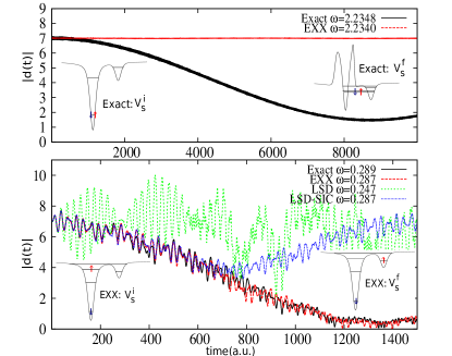
Figure 1: Dipole moments calculated from the center of the double-well: exact (black), EXX (red), LSD (green) and SIC-LSD (blue), driven at resonant $\omega^{i}$ for each. The initial and target-final KS potentials are shown as insets, exact in the top panel, and in EXX in the lower panel. Top panel: CT from the ground-state. Lower panel: CT from the “photo-excited” state.

	$\omega_{\scriptscriptstyle\rm S}^{i}$	$\omega_{\scriptscriptstyle\rm S}^{f}$	$\omega_{\scriptscriptstyle\rm S}^{\rm g.s.}$	TDDFT $\omega^{i}$	TDDFT $\omega^{f}$
EXX	0.286	0.286	0.288	0.287	0.287
LSD	0.247	0.094	0.482	–	0.091
SIC-LSD	0.287	0.236	0.267	0.287	0.237

Table 1: Bare KS and TDDFT-corrected photo-excited CT frequencies computed in the initial, targeted final, and ground states, in atomic units (au). The exact CT frequency is $\omega=0.289$ au. The TDDFT values were obtained via linear response to a $\delta-$kick perturbation Yabana et al. (2006) and “–” indicates no peak was discernible in the spectra, but we expect $\omega^{i}\approx\omega_{\scriptscriptstyle\rm S}^{i}$. Calculations were performed using the octopus code Andrade et al. (2012); Castro et al. (2006): a box of size 50 au, grid spacing 0.1au, and time-step 0.005au were used.

In a third example, when resonantly driving between two locally excited states in a single well ($v_{\rm ext}=-2/\sqrt{(}x^{2}+1)-3/\cosh^{2}x$), one finds again that the EXX frequencies computed from each excited state are very similar, $0.824$au, quite different than the exact resonant frequency of $0.755$au. Despite this large discrepancy, the EXX dipole closely follows the exact one, due to the approximate satisfaction of condition (8), and, likely, condition (7), LSD again violates condition (8) the most severely, and its dynamics is consequently the worst.

Interestingly, our exact condition could explain the success of the “instantaneous ground-state” approximation over the adiabatic approximation, explored in Ref. Mancini et al. (2014): there, for initial non-stationary states evolving in a time-independent external field, the KS potential is always taken as equal to the initial one, so has static resonances, satisfying Eq. (7).

In conclusion, we have derived a new exact condition that should be satisfied by approximate functionals in TDDFT in order to accurately capture non-equilibrium dynamics. Violations of this condition lead to misleading results in simulating time-resolved spectroscopy, and failure in resonantly driven processes. We have shown that even if a functional does not yield accurate excitation frequencies, if these frequencies even approximately satisfy the exact condition Eq. (7) then the predicted non-linear dynamics could still be accurate. The effect of the spurious time-dependent resonances of approximate functionals for realistic systems could be dampened, due to the large number of electrons and vibronic couplings, but further investigations are necessary. Likely for spectroscopy or resonant control processes, satisfaction of the exact condition is essential, and our findings explain related observations in the real systems studied in Refs. Ramakrishnan and Nest (2012); Raghunathan and Nest (2012); Habenicht et al. (2014); De Giovannini et al. (2013). The exact condition highlights a new feature that must be considered in the development of improved functionals to be able to accurately capture dynamics far from the ground-state.