Rigidity results with applications to best constants and symmetry of Caffarelli-Kohn-Nirenberg and logarithmic Hardy inequalities

Abstract

We take advantage of a rigidity result for the equation satisfied by an extremal function associated with a special case of the Caffarelli-Kohn-Nirenberg inequalities to get a symmetry result for a larger set of inequalities. The main ingredient is a reparametrization of the solutions to the Euler-Lagrange equations and estimates based on the rigidity result. The symmetry results cover a range of parameters which go well beyond the one that can be achieved by symmetrization methods or comparison techniques so far.

2010 Mathematics Subject Classification. 26D10 46E35 35J20 49J40

1 Introduction and main results

Let $2^{*}:=\infty$ if $d=1$, $2$, and $2^{*}:=2\,d/(d-2)$ if $d\geq 3$. Define

$$\vartheta(p,d):=\frac{d\,(p-2)}{2\,p},\hskip 42.67912pta_{c}:=\frac{d-2}{2}\ ,$$

and consider the space $\mathcal{D}_{a}^{1,2}({\mathbb{R}}^{d})$ obtained by completion of $\mathcal{D}({\mathbb{R}}^{d}\setminus\{0\})$ with respect to the norm $v\mapsto\|{\,|x|^{-a}\,\nabla v\,}\|_{\mathrm{L}^{2}({\mathbb{R}}^{d})}^{2}$. We will be concerned with the following two families of inequalities

Caffarelli-Kohn-Nirenberg Inequalities (CKN) Caffarelli-Kohn-Nirenberg-84 Let $d\geq 1$. For any $p\in[2,2^{*}]$ if $d\geq 3$ or $p\in[2,2^{*})$ if $d=1$, $2$, for any $\theta\in[\vartheta(p,d),1]$ with $\theta>1/2$ if $d=1$, there exists a positive constant $\mathsf{C}_{\rm CKN}(\theta,p,a)$ such that

$$\left(\;\int_{{\mathbb{R}}^{d}}{\frac{|v|^{p}}{|x|^{b\,p}}}\;dx\right)^{\frac{2}{p}}\leq\mathsf{C}_{\rm CKN}(\theta,p,a)\left(\;\int_{{\mathbb{R}}^{d}}{\frac{|\nabla v|^{2}}{|x|^{2\,a}}}\;dx\right)^{\!\theta}\left(\;\int_{{\mathbb{R}}^{d}}{\frac{|v|^{2}}{|x|^{2\,(a+1)}}}\;dx\right)^{\!1-\theta}$$ (1)

holds true for any $v\in\mathcal{D}^{1,2}_{a}({\mathbb{R}}^{d})$. Here $a$, $b$ and $p$ are related by $b=a-a_{c}+d/p$, with the restrictions $a\leq b\leq a+1$ if $d\geq 3$, $a<b\leq a+1$ if $d=2$ and $a+1/2<b\leq a+1$ if $d=1$. Moreover, the constants $\mathsf{C}_{\rm CKN}(\theta,p,a)$ are uniformly bounded outside a neighborhood of $a=a_{c}$.

In DDFT , a new class of inequalities, called weighted logarithmic Hardy inequalities, was considered. These inequalities can be obtained from (1) by taking $\theta=\gamma\,(p-2)$ and passing to the limit as $p\to 2_{+}$.

Weighted Logarithmic Hardy Inequalities (WLH)DDFT Let $d\geq 1$, $a<a_{c}$, $\gamma\geq d/4$ and $\gamma>1/2$ if $d=2$. Then there exists a positive constant $\mathsf{C}_{\rm WLH}(\gamma,a)$ such that, for any $v\in\mathcal{D}^{1,2}_{a}({\mathbb{R}}^{d})$ normalized by

$$\int_{{\mathbb{R}}^{d}}{|x|^{-2\,(a+1)}\,|v|^{2}}\;dx=1\ ,$$

we have

$$\int_{{\mathbb{R}}^{d}}{\frac{|v|^{2}}{|x|^{2\,(a+1)}}\,\log\left(|x|^{2\,(a_{c}-a)}\,|v|^{2}\right)}\;dx\leq 2\,\gamma\,\log\left[\mathsf{C}_{\rm WLH}(\gamma,a)\int_{{\mathbb{R}}^{d}}{\frac{|\nabla v|^{2}}{|x|^{2\,a}}}\;dx\right].$$ (2)

Moreover, the constants $\mathsf{C}_{\rm WLH}(\gamma,a)$ are uniformly bounded outside a neighborhood of $a=a_{c}$.

It is very convenient to reformulate the Caffarelli-Kohn-Nirenberg inequality in cylindrical variables as in Catrina-Wang-01 . By means of the Emden-Fowler transformation

$$s=\log|x|\in{\mathbb{R}}\ ,\quad\omega=\frac{x}{|x|}\in{\mathbb{S}^{d-1}}\ ,\quad y=(s,\omega)\ ,\quad u(y)=|x|^{a_{c}-a}\,v(x)\ ,$$

Inequality (1) for $v$ is equivalent to a Gagliardo-Nirenberg-Sobolev inequality for the function $u$ on the cylinder $\mathcal{C}:={\mathbb{R}}\times{\mathbb{S}^{d-1}}$:

$$\mathsf{K}_{\rm CKN}(\theta,p,\Lambda)\,\|{u}\|_{\mathrm{L}^{p}(\mathcal{C})}^{2}\leq\left(\|{\nabla u}\|_{\mathrm{L}^{2}(\mathcal{C})}^{2}\!+\!\Lambda\,\|{u}\|_{\mathrm{L}^{2}(\mathcal{C})}^{2}\right)^{\theta}\|{u}\|_{\mathrm{L}^{2}(\mathcal{C})}^{2\,(1-\theta)}\quad\kern-1.66pt\forall\,u\in\mathrm{H}^{1}(\mathcal{C})\ .$$ (3)

Here and throughout the rest of the work we set

$$\Lambda:=(a_{c}-a)^{2}\ .$$

Similarly, with $u(y)=|x|^{a_{c}-a}\,v(x)$, Inequality (2) is equivalent to

$$\int_{\mathcal{C}}{|u|^{2}\,\log|u|^{2}}\;dy\leq 2\,\gamma\,\log\left[\frac{1}{\mathsf{K}_{\rm WLH}(\gamma,\Lambda)}\Big{(}\|{\nabla u}\|_{\mathrm{L}^{2}(\mathcal{C})}^{2}+\Lambda\Big{)}\right]\ ,$$ (4)

for any $u\in\mathrm{H}^{1}(\mathcal{C})$ such that $\|{u}\|_{\mathrm{L}^{2}(\mathcal{C})}=1$. In both cases, we consider on $\mathcal{C}$ the measure $d\mu=|{\mathbb{S}^{d-1}}|^{-1}d\omega\,ds$ obtained by normalizing the surface of ${\mathbb{S}^{d-1}}$ to $1$ (that is, the uniform probability measure), tensorized with the usual Lebesgue measure on the axis of the cylinder.

We are interested in symmetry and symmetry breaking issues: when do we know that equality in (1) and (2) is achieved by radial functions or, alternatively, by functions depending only on $s$ in (3) and (4)? Related with inequality (3) is the Rayleigh quotient:

$$\mathcal{Q}_{\Lambda}^{\theta}[u]:=\frac{\left(\|{\nabla u}\|_{2}^{2}+\Lambda\,\|{u}\|_{2}^{2}\right)^{\theta}\,\|{u}\|_{2}^{2\,(1-\theta)}}{\|{u}\|_{p}^{2}}\ .$$

Here $\|{u}\|_{q}:=\left(\int_{\mathcal{C}}{|u|^{q}}\;d\mu\right)^{1/q}$. Then (3) and (4) are equivalent to state that

$$\mathsf{K}_{\rm CKN}(\theta,p,\Lambda)=\inf_{u\in\mathrm{H}^{1}(\mathcal{C})\setminus\{0\}}\mathcal{Q}_{\Lambda}^{\theta}[u]\ ,$$

$$\mathsf{K}_{\rm WLH}(\gamma,\Lambda)=\inf_{\begin{array}[]{c}\scriptstyle u\in\mathrm{H}^{1}(\mathcal{C})\setminus\{0\}\cr\scriptstyle\|{u}\|_{2}=1\end{array}}\left(\|{\nabla u}\|_{2}^{2}+\Lambda\right)\,e^{-\frac{1}{2\,\gamma}\int_{\mathcal{C}}{|u|^{2}\,\log|u|^{2}}\;d\mu}\ .$$

Let $\mathsf{K}_{\rm CKN}^{*}(\theta,p,\Lambda)$ and $\mathsf{K}_{\rm WLH}^{*}(\gamma,\Lambda)$ be the corresponding values of the infimum when the set of minimization is restricted to functions depending only on $s$. The main interest of introducing the measure $d\mu$ is that $\mathsf{K}_{\rm CKN}^{*}(\theta,p,\Lambda)$ and $\mathsf{K}_{\rm WLH}^{*}(\gamma,\Lambda)$ are independent of the dimension and can be computed for $d=1$ by solving the problem on the real line ${\mathbb{R}}$.

Radial symmetry of $v=v(x)$ means that $u=u(s,\omega)$ is independent of $\omega$. Up to translations in $s$ and a multiplication by a constant, the optimal functions in the class of functions depending only on $s\in{\mathbb{R}}$ solve the equation

$$-u_{*}^{\prime\prime}+\Lambda\,u_{*}=u_{*}^{p-1}\quad\mbox{in}\quad{\mathbb{R}}$$

if $\theta=1$. See Section 2 if $\theta<1$. Up to translations in $s$, non-negative solutions of this equation are all equal to the function

$$u_{*}(s):=\frac{A}{\big{[}\cosh(B\,s)\big{]}^{\frac{2}{p-2}}}\quad\forall\,s\in{\mathbb{R}}\ ,$$ (6)

with $A^{p-2}=\tfrac{p}{2}\,\Lambda$ and $B=\tfrac{1}{2}\,\sqrt{\Lambda}\,(p-2)$. The uniqueness up to translations is a standard result (see for instance (Dolbeault06082014, , Proposition B.2) for a proof).

The symmetry breaking issue is now reduced to the question of knowing whether the inequalities

$$\mathsf{K}_{\rm CKN}(\theta,p,\Lambda)\leq\mathsf{K}_{\rm CKN}^{*}(\theta,p,\Lambda)\quad\mbox{and}\quad\mathsf{K}_{\rm WLH}(\gamma,\Lambda)\leq\mathsf{K}_{\rm WLH}^{*}(\gamma,\Lambda)$$ (7)

are strict or not, when $d\geq 2$. Symmetry breaking occurs if the inequality is strict and then optimal functions are not symmetric (symmetric means: depending only on $s$ in the setting of the cylinder, or on $|x|$ in the case of the Euclidean space). In (DDFT, , pp. 2048 and 2057), the values of the symmetric constants have been computed. They are given by

$$\textstyle\mathsf{K}_{\rm CKN}^{*}(\theta,p,\Lambda):=\left[\frac{2p\theta+2-p}{(p-2)^{2}}\right]^{\frac{p-2}{2\,p}}\left[\frac{2p\theta}{2p\theta+2-p}\right]^{\theta}\left[\frac{p+2}{4}\right]^{\frac{6-p}{2\,p}}\left[\frac{\sqrt{\pi}\;\Gamma\left(\frac{2}{p-2}\right)}{\Gamma\left(\frac{2}{p-2}+\frac{1}{2}\right)}\right]^{\frac{p-2}{p}}\kern-5.0pt\Lambda^{\theta-\frac{p-2}{2\,p}}$$ (8)

and

$$\textstyle\mathsf{K}_{\rm WLH}^{*}(\gamma,\Lambda)=\frac{\gamma\,\left(8\pi^{d+1}\,e\right)^{\frac{1}{4\gamma}}}{\Gamma\left(\frac{d}{2}\right)^{\frac{1}{2\gamma}}}\,\left(\frac{4\Lambda}{4\gamma-1}\right)^{\frac{4\gamma-1}{4\gamma}}\;\mbox{if}\;\gamma>\frac{1}{4}\ ,$$

$$\textstyle\mathsf{K}_{\rm WLH}^{*}(\gamma,\Lambda)=\frac{2\pi^{d+1}\,e}{\Gamma\left(\frac{d}{2}\right)^{2}}\;\;\;\;\;~{}~{}~{}~{}~{}~{}~{}~{}~{}~{}\mbox{if}\;\;~{}\;\gamma=\frac{1}{4}\ .$$

Let

$$\textstyle\Lambda_{\rm FS}(\theta,p,d):=4\,\frac{d-1}{p^{2}-4}\,\frac{(2\,\theta-1)\,p+2}{p+2}\quad\mbox{and}\quad\Lambda_{\star}(1,p,d):=\frac{1}{4}\,(d-1)\,\frac{6-p}{p-2}\ .$$ (9)

We will define $\Lambda_{\star}(\theta,p,d)$ for $\theta<1$ later in the Introduction. Symmetry breaking occurs for any $\Lambda>\Lambda_{\rm FS}$ according to a result of V. Felli and M. Schneider in Felli-Schneider-03 for $\theta=1$ and in DDFT for $\theta<1$ (also see Catrina-Wang-01 for previous results and MR2437030 if $d=2$ and $\theta=1$). This symmetry breaking is a straightforward consequence of the fact that for $\Lambda>\Lambda_{\rm FS}$, the symmetric optimals are saddle points of an energy functional, and thus cannot be even local minima. As a consequence, we know that $\mathsf{K}_{\rm CKN}(\theta,p,\Lambda)<\mathsf{K}_{\rm CKN}^{*}(\theta,p,\Lambda)$ if $\Lambda>\Lambda_{\rm FS}(\theta,p,d)$.

Concerning the log Hardy inequality, it was shown in DDFT that symmetry breaking occurs, that is, $\mathsf{K}_{\rm WLH}(\gamma,\Lambda)<\mathsf{K}_{\rm WLH}^{*}(\gamma,\Lambda)$, when either $d=2$ and $\gamma>1/2$ or $d\geq 3$ and $\gamma\geq d/4$ provided that

$$\Lambda>(d-1)\left(\gamma-\tfrac{1}{4}\right)\ .$$

Concerning symmetry, if $\theta=1$, from DEL2011 , we know that symmetry holds for CKN for any $\Lambda\leq\Lambda_{\star}(1,p,d)$. The precise statement goes as follows.

Theorem 1.1

DEL2011 Let $d\geq 2$. For any $p\in[2,2^{*}]$ if $d\geq 3$ or $p\in[2,\infty)$ if $d=2$, under the conditions

$$0<\mu\leq\Lambda_{\star}(1,p,d)\hskip 22.76219pt{\rm and}\hskip 22.76219pt\mathcal{Q}_{\mu}^{1}[u]\leq\mathsf{K}_{\rm CKN}^{*}(1,p,\mu)\ ,$$

the solution of

$$-\,\Delta u+\mu\,u=u^{p-1}\quad\mbox{on}\quad\mathcal{C}$$ (10)

is given by the one-dimensional equation, written on ${\mathbb{R}}$. It is unique, up to translations.

Theorem 1.1 is a rigidity result. In DEL2011 , the proof is given for a minimizer of $\mathcal{Q}_{\mu}^{1}$, which therefore satisfies $\mathcal{Q}_{\mu}^{1}[u]\leq\mathsf{K}_{\rm CKN}^{*}(1,p,\mu)$, but the reader is invited to check that only the latter condition is used in the proof. The proof is based on a chain of estimates which involve optimal interpolation inequalities on the sphere and the Keller-Lieb-Thirring inequality. These inequalities turn out to be equalities, and equality in each of the inequalities is shown to imply that the solution only depends on $s$ (no angular dependence). The result of Theorem 1.1 gives a sufficient condition for symmetry when $\theta=1$. We shall say that any minimizer is symmetric if it is given by (6), up to multiplications by constants and translations.

Theorem 1.2

DEL2011 Let $d\geq 2$. For any $p\in[2,2^{*}]$ if $d\geq 3$ or any $p\in[2,\infty)$ if $d=2$, if $0<\Lambda\leq\Lambda_{\star}(1,p,d)$, then $\mathsf{K}_{\rm CKN}(1,p,\Lambda)=\mathsf{K}_{\rm CKN}^{*}(1,p,\Lambda)$ and any minimizer is symmetric.

In DEL2011 , the case $\theta<1$ is also considered. According to (DEL2011, , Theorem 9), for any $d\geq 3\,$, any $p\in(2,2^{*})$ and any $\theta\in[\vartheta(p,d),1)\,$, we have the estimate

$$\mathfrak{C}(\theta,p)^{-\frac{2\,\theta}{q+2}}\,\mathsf{K}_{\rm CKN}^{*}(\theta,\Lambda,p)\leq\mathsf{K}_{\rm CKN}(\theta,\Lambda,p)\leq\mathsf{K}_{\rm CKN}^{*}(\theta,\Lambda,p)$$ (11)

where $q:=\frac{2\,(p-2)}{(2\,\theta-1)\,p+2}$ and

$$\mathfrak{C}(\theta,p):=\tfrac{(p+2)^{\frac{p+2}{(2\,\theta-1)\,p+2}}}{(2\,\theta-1)\,p+2}\,\left(2-\tfrac{p}{2}\,(1-\theta)\right)^{1-\frac{q}{2}}\\ \cdot\left(\frac{\Gamma(\frac{p}{p-2})}{\Gamma(\frac{\theta\,p}{p-2})}\right)^{\!2\,q}\,\left(\frac{\Gamma(\frac{2\,\theta\,p}{p-2})}{\Gamma(\frac{2\,p}{p-2})}\right)^{\!q}$$

under the condition $a_{c}^{2}<\Lambda\leq\frac{(d-1)}{\mathfrak{C}(\theta,p)}\,\frac{(2\,\theta-3)\,p+6}{4\,(p-2)}$. If $\theta=1$, the equality case in the last inequality characterizes $\Lambda_{\star}(1,p,d)$ as defined in (9). However (11) does not give a range for symmetry unless $\theta=1$.

Much more is known. According to DELT09 ; springerlink:10.1007/s00526-011-0394-y , there is a continuous curve $p\mapsto\Lambda_{\rm s}(\theta,p,d)$ with $\lim_{p\to 2_{+}}\Lambda_{\rm s}(\theta,p,d)=\infty$ and $\Lambda_{\rm s}(\theta,p,d)>a_{c}^{2}$ for any $p\in(2,2^{*})$ such that symmetry holds for any $\Lambda\leq\Lambda_{\rm s}(1,p,d)$ and there is symmetry breaking if $\Lambda>\Lambda_{\rm s}(1,p,d)$, for any $\theta\in[\vartheta(p,d),1)$. Additionally, we have that $\lim_{p\to 2^{*}}\Lambda_{\rm s}(1,p,d)=a_{c}^{2}$ if $d\geq 3$ and, if $d=2$, $\lim_{p\to\infty}\Lambda_{\rm s}(1,p,d)=0$ and $\lim_{p\to\infty}p^{2}\Lambda_{\rm s}(1,p,d)=4$. The existence of this function $\Lambda_{\rm s}$ has been proven in an indirect way, and it is not explicitly known. It has been a long-standing question to decide whether the curves $p\to\Lambda_{\rm s}(\theta,p,d)$ and the curve $p\to\Lambda_{\rm FS}(\theta,p,d)$ coincide or not. This is still an open question, at least for $\theta=1$. For $\theta<1$, and for some specific values of $p$, it has been shown that, in some cases, $\Lambda_{\rm s}(\theta,p,d)<\Lambda_{\rm FS}(\theta,p,d)$; see springerlink:10.1007/s00526-011-0394-y for more details, as well as some symmetry results based on symmetrization techniques. A scenario based on numerical computations and asymptotic expansions at the point where non-symmetric positive solutions bifurcate from the symmetric ones has been proposed; see Oslo ; Freefem ; DE2012 for details.

Our interest in this work is to establish symmetry of the minimizers of CKN for $\theta<1$ as well as of the log Hardy inequalities, thus identifying the corresponding sharp constants.

Our first result is an extension of Theorem 1.2 to the case $\theta<1$. Our goal is to give explicit estimates of the range for which symmetry holds. This requires some notations and a preliminary result. We set

$$\Pi^{*}(\theta,p,q):=\left(\frac{\mathsf{K}_{\rm CKN}^{*}(\theta,p,1)}{\mathsf{K}_{\rm CKN}^{*}(1,q,1)^{\frac{q\,(p-2)}{p\,(q-2)}}}\right)^{\frac{1}{\theta-\frac{q\,(p-2)}{p\,(q-2)}}}\ .$$ (12)

Next we define

$$q^{*}=q^{*}(\theta,p):=\frac{2\,p\,\theta}{2-p\,(1-\theta)}\ .$$ (13)

The condition $\theta>\frac{q\,(p-2)}{p\,(q-2)}$ is equivalent to $q>q^{*}(\theta,p)$ and we can notice that $p<q^{*}(\theta,p)<2^{*}$ for any $\theta\in(\vartheta(p,d),1)$. For $d\geq 3$ we define

$$\Lambda_{1}(\theta,p,d):=\max_{q\in(q^{*},2^{*})}\;\min\left\{\Lambda_{\star}(1,q,d),\frac{\theta\,\Lambda_{\star}(1,p,d)}{(1-\theta)\,\Pi^{*}(\theta,p,q)+\theta}\right\}\ ,$$

whereas for $d=2$

$$\Lambda_{1}(\theta,p,2):=\max_{q\in(q^{*},6)}\;\min\left\{\Lambda_{\star}(1,q,2),\frac{\theta\,\Lambda_{\star}(1,p,2)}{(1-\theta)\,\Pi^{*}(\theta,p,q)+\theta}\right\}\ .$$

Next, we can also define

$$\mathsf{N}(\theta,p):=\frac{\big{(}\mathsf{K}_{\rm CKN}^{*}(\theta,p,1)\big{)}^{1/\theta}}{\mathsf{K}_{\rm CKN}^{*}\big{(}1,q^{*}(\theta,p),1\big{)}}\ .$$ (14)

We refer to Section 3 for an explicit expression of $\mathsf{N}(\theta,p)$. We introduce the exponent

$$\beta=\beta(\theta,p):=1-\frac{p-2}{2\,p\,\theta}\ .$$ (15)

For $2<p<6$ and $\theta\in(\vartheta(p,3),1)$ we denote by $\mathsf{x}^{*}=\mathsf{x}^{*}(\theta,p)$ the unique root of the equation

$$\theta\,(6-p)\big{(}x^{\beta}-\mathsf{N}\big{)}\,x-\big{(}2\,p\,\theta-3\,(p-2)\big{)}\left(\theta\,\big{(}x^{\beta}-\mathsf{N}\big{)}+(1-\theta)\,(x-1)\,\mathsf{N}\right)=0\ ,$$

in the interval $(\mathsf{N}^{1/\beta},\infty)$ for $\mathsf{N}=\mathsf{N}(\theta,p)$, see Lemma 2 in Section 3. Next we define

$$\Lambda_{2}(\theta,p,d):=\frac{\Lambda_{\star}(1,q^{*},d)}{\mathsf{x}^{*}(\theta,p)}=\frac{1}{4}\,(d-1)\,\frac{2\,p\,\theta-3\,(p-2)}{(p-2)\,\mathsf{x}^{*}(\theta,p)}\ ,$$

and

$$\Lambda_{\star}(\theta,p,d):=\max\Big{\{}\Lambda_{1}(\theta,p,d),\Lambda_{2}(\theta,p,d)\Big{\}}\ .$$

Theorem 1.3

Suppose that either $d=2$ and $p\in(2,6)$ or else $d\geq 3$ and $p\in(2,2^{*})$. Then

$$\mathsf{K}_{\rm CKN}(\theta,p,\Lambda)=\mathsf{K}_{\rm CKN}^{*}(\theta,p,\Lambda)\ ,$$

and any minimizer of CKN (3) is symmetric provided that one of the following conditions is satisfied:

1. $d=2$, $\theta\in(\vartheta(p,2),1)$ and $0<\Lambda\leq\Lambda_{1}(\theta,p,2)$.

2. $d=2$, $\theta\in(\vartheta(p,3),1)$ and $0<\Lambda\leq\Lambda_{\star}(\theta,p,2)$,

3. $d\geq 3$, $\theta=\vartheta(p,d)$ and $0<\Lambda\leq\Lambda_{2}(\theta,p,d)$,

4. $d\geq 3$, $\theta\in(\vartheta(p,d),1)$ and $0<\Lambda\leq\Lambda_{\star}(\theta,p,d)$  .

Our definition of $\Lambda_{\star}(\theta,p,d)$ for $\theta<1$ is consistent with the definition of $\Lambda_{\star}(1,p,d)$ given in (9) because

$$\lim_{\theta\to 1}\Lambda_{1}(\theta,p,d)=\lim_{\theta\to 1}\Lambda_{2}(\theta,p,d)=\Lambda_{\star}(1,p,d)\ .$$

One of the drawbacks in the definition of $\Lambda_{2}(\theta,p,d)$ is that $\mathsf{x}^{*}(\theta,p)$ given by Lemma 2 is not explicit. For an explicit estimate of $\Lambda_{2}(\theta,p,d)$ see Proposition 2 in Section 5.

By passing to the limit as $p\to 2_{+}$ in the criterion $\Lambda\leq\Lambda_{2}(\theta,p,d)$, we also obtain an explicit condition for symmetry in the weighted logarithmic Hardy inequalities. For any $\mathsf{N}_{0}>1$, consider the smallest root $x>\mathsf{N}_{0}^{1/\beta_{0}}$ of

$$4\,\gamma\,x^{\beta_{0}+1}-(8\,\gamma-3)\,\mathsf{N}_{0}\,x+(4\,\gamma-3)\,\mathsf{N}_{0}\,=0\quad\mbox{with}\quad\beta_{0}=1-\frac{1}{4\,\gamma}$$

and denote it by $\mathsf{x}_{0}^{*}(\gamma)$ if $\mathsf{N}_{0}=\mathsf{N}_{0}(\gamma):=\lim_{p\to 2_{+}}\mathsf{N}(\gamma\,(p-2),p)$. An elementary but tedious computation shows that

$$\mathsf{N}_{0}(\gamma)=2^{1-\frac{3}{4\,\gamma}}\,e^{\frac{1}{4\,\gamma}}\,\frac{(2\,\gamma-1)^{1-\frac{1}{\gamma}}}{(4\,\gamma-1)^{1-\frac{3}{4\,\gamma}}}\left(\frac{\Gamma\left(2\,\gamma-\frac{1}{2}\right)}{\Gamma\left(2\,\gamma-1\right)}\right)^{\!\frac{1}{2\,\gamma}}.$$ (16)

Let us define

$$\Lambda_{0}(\gamma,d):=\frac{(d-1)\,\left(\gamma-3/4\right)}{\mathsf{x}_{0}^{*}(\gamma)}\ .$$ (17)

We then have

Theorem 1.4

Assume that either $d=2$ or $3$ and $\gamma>3/4$, or $d\geq 4$ and $\gamma\geq d/4$. Then

$$\textstyle\mathsf{K}_{\rm WLH}(\gamma,\Lambda)=\textstyle\mathsf{K}_{\rm WLH}^{*}(\gamma,\Lambda)\ ,$$

and any minimizer of (4) is symmetric provided that

$$0<\Lambda\leq\Lambda_{0}(\gamma,d)\ .$$

For an explicit estimate of $\Lambda_{0}(\gamma,d)$ see Proposition 3 in Section 5.

Theorem 1.3 provides us with a rigidity result, which is stronger than a simple symmetry result. As a consequence, our estimates of Theorem 1.3 for the symmetry region cannot be optimal.

Theorem 1.5

Suppose that either $d=2$ and $p\in(2,6)$ or else $d\geq 3$ and $p\in(2,2^{*})$. If $\theta>\vartheta(p,\min\{3,d\})$, then

$$\Lambda_{\star}(\theta,p,d)<\Lambda_{\rm s}(\theta,p,d)\leq\Lambda_{\rm FS}(\theta,p,d)\ .$$

If either $d=3$ and $\theta=\vartheta(p,3)$, or $d=2$ and $\theta>0$, then

$$\Lambda_{2}(\theta,p,d)<\Lambda_{\rm s}(\theta,p,d)\leq\Lambda_{\rm FS}(\theta,p,d)\ .$$

It can be conjectured that $\Lambda_{\rm s}(\theta,p,d)=\Lambda_{\rm FS}(\theta,p,d)$ holds in the limit case $\theta=1$, and probably also for $\theta$ close enough to $1$, on the basis of the numerical results of Freefem and the formal computations of DE2012 . On the other hand, it is known from springerlink:10.1007/s00526-011-0394-y that $\Lambda_{\rm s}(\theta,p,d)<\Lambda_{\rm FS}(\theta,p,d)$ when $\theta-\vartheta(p,d)$ is small enough, at least for some values of $p$ and $d$.

The expressions involved in the statement of Theorem 1.3 look quite technical, but they are interesting for two reasons:

• Theorem 1.3 determines a range for symmetry which goes well beyond what can be achieved using standard methods and is somewhat unexpected in view of the estimate of (DEL2011, , Theorem 9). It is a striking observation that the reparametrization method which has been extensively used in Freefem ; DE2012 allows us to extend to $\theta<1$ results which were known only for $\theta=1$.

• Even if they cannot be optimal as shown in Theorem 1.5, the estimates of Theorem 1.3 are rather accurate from the numerical point of view, as will be illustrated in Section 5.

This paper is organized as follows. Section 2 is devoted to the reparametrization and the proof of symmetry when $\Lambda\leq\Lambda_{1}(\theta,p,d)$ in the subcritical case $\vartheta(p,d)<\theta<1$. To the price of some additional technicalities, the range $\Lambda\leq\Lambda_{2}(\theta,p,d)$ and $\vartheta(p,\min\{3,d\})\leq\theta<1$ is covered in Section 3. The proofs of Theorems 1.3 and 1.5 are established in Section 4. The last section is devoted to an explicit approximation of $\Lambda_{0}$ and $\Lambda_{2}$, and some numerical results which illustrate Theorems 1.3 and 1.5. The reader interested in the strategy of the proofs as well as the origin of the expressions of $\Lambda_{1}(\theta,p,d)$ and $\Lambda_{2}(\theta,p,d)$ is invited to read first Section 2 and the proof of Lemma 5 in Section 3.

2 Reparametrization and a first symmetry result

We begin by a reparametrization of the branches of the solutions which allows us to reduce the case corresponding to $\theta<1$ and $\Lambda$ to the case corresponding to $\theta=1$ and some related $\mu$, as in Theorem 1.1. Consider an optimal function $u$ for (3), which therefore satisfies

$$\mathsf{K}_{\rm CKN}(\theta,p,\Lambda)=\mathcal{Q}_{\Lambda}^{\theta}[u]=(t+\Lambda)^{\theta}\,\frac{\|{u}\|_{2}^{2}}{\|{u}\|_{p}^{2}}\quad\mbox{with}\quad t:=\frac{\|{\nabla u}\|_{2}^{2}}{\|{u}\|_{2}^{2}}\ .$$

According to (springerlink:10.1007/s00526-011-0394-y, , Theorem1), such a function $u$ exists for any $\theta>\vartheta(p,d)$. As a critical point of $\mathcal{Q}_{\Lambda}^{\theta}$, $u$ solves (10) with

$$\theta\,\mu=(1-\theta)\,t+\Lambda$$

if it has been normalized by the condition

$$\|{\nabla u}\|_{2}^{2}+\Lambda\,\|{u}\|_{2}^{2}=\theta\,\|{u}\|_{p}^{p}\ .$$

Because of the zero-homogeneity of $\mathcal{Q}_{\Lambda}^{\theta}$, such a condition can be imposed without restriction and is equivalent to

$$\|{u}\|_{2}^{2}=\frac{\theta}{t+\Lambda}\,\|{u}\|_{p}^{p}\ .$$ (18)

Proposition 1

Let us assume that $u$ is a solution of (10), satisfying $\mathcal{Q}_{\Lambda}^{\theta}[u]=\mathsf{K}_{\rm CKN}(\theta,p,\Lambda)$ and (18), with $\theta\,\mu=(1-\theta)\,t+\Lambda$. Then we have

$$\mathcal{Q}_{\mu}^{1}[u]\leq\mathsf{K}_{\rm CKN}^{*}(1,p,\mu)\ .$$ (19)

Proof

From (7) we know that

$$(t+\Lambda)^{\theta}\,\frac{\|{u}\|_{2}^{2}}{\|{u}\|_{p}^{2}}\leq\mathsf{K}_{\rm CKN}^{*}(\theta,p,\Lambda)\ .$$

Using (18), we rewrite this estimate as

$$\theta\,(t+\Lambda)^{\theta-1}\,\|u\|_{p}^{p-2}\leq\mathsf{K}_{\rm CKN}^{*}(\theta,p,\Lambda)\ .$$

Using (18) again and the expression of $\mu$, we obtain

$$Q^{1}_{\mu}[u]=\frac{\theta\,(t+\mu)}{t+\Lambda}\,\|u\|_{p}^{p-2}=\|u\|_{p}^{p-2}\leq f(t,\theta,\Lambda,p)\,\mathsf{K}_{\rm CKN}^{*}(1,p,\mu)$$

with

$$f(t,\theta,\Lambda,p):=\frac{1}{\theta\,(t+\Lambda)^{\theta-1}}\,\frac{\mathsf{K}_{\rm CKN}^{*}(\theta,p,\Lambda)}{\mathsf{K}_{\rm CKN}^{*}(1,p,\mu)}\ .$$

Using the expression of $\mu$ and (8), we find that

$$f(t,\theta,\Lambda,p)=\tfrac{(p+2)^{\frac{p+2}{2\,p}}}{(2\,p)^{1-\theta}}\,\big{(}\tfrac{\Lambda\,\theta}{2+(2\,\theta-1)\,p}\big{)}^{\theta-\frac{p-2}{2\,p}}\,(t+\Lambda)^{1-\theta}\,\big{(}(1-\theta)\,t+\Lambda\big{)}^{-\frac{p+2}{2\,p}}$$

achieves its maximum at $t_{0}:=\Lambda\,\big{(}\frac{2\,p\,\theta}{p-2}-1\big{)}^{-1}>0$. Hence $f(t)\leq f(t_{0})=1$, which concludes the proof.

Using the notations (12) and (13), we obtain our first symmetry result, which goes as follows.

Lemma 1

Suppose that either $d=2$ and $p\in(2,6)$ or else $d\geq 3$, $p\in(2,2^{*})$. If $\theta\in(\vartheta(p,d),1)$ and

$$\Lambda\leq\min\left\{\Lambda_{\star}(1,q,d),\frac{\theta\,\Lambda_{\star}(1,p,d)}{(1-\theta)\,\Pi^{*}(\theta,p,q)+\theta}\right\}$$

for some $q\in\big{(}q^{*}(\theta,p),6)$ when $d=2$, or for some $q\in\big{(}q^{*}(\theta,p),2^{*}\big{)}$ when $d\geq 3$, then any optimal function for (3) is symmetric.

Proof

Let $u$ be a solution as in Proposition 1. From (7), we know that

$$\mathsf{K}_{\rm CKN}^{*}(\theta,p,\Lambda)\geq(t+\Lambda)^{\theta}\,\frac{\|{u}\|_{2}^{2}}{\|{u}\|_{p}^{2}}\ .$$

For $p<q<\min\{6,2^{*}\}$ we have by Hölder’s inequality, $\|{u}\|_{p}\leq\|{u}\|_{2}^{\delta}\,\|{u}\|_{q}^{1-\delta}$ provided $\delta=\frac{2}{p}\,\frac{q-p}{q-2}$, and thus $1-\delta=\frac{q}{p}\,\frac{p-2}{q-2}$. Hence

$$\mathsf{K}_{\rm CKN}^{*}(\theta,p,\Lambda)\geq(t+\Lambda)^{\theta}\,\left(\frac{\|{u}\|_{2}^{2}}{\|{u}\|_{q}^{2}}\right)^{1-\delta}\ .$$

Now, for any $\lambda\in(0,\Lambda_{\star}(1,q,d)]$, we know from Theorem 1.2 that

$$\|{u}\|_{q}^{2}\leq\frac{\|{\nabla u}\|_{2}^{2}+\lambda\,\|{u}\|_{2}^{2}}{\mathsf{K}_{\rm CKN}^{*}(1,q,\lambda)}\ ,$$

which shows that

$$\mathsf{K}_{\rm CKN}^{*}(\theta,p,\Lambda)\geq(t+\Lambda)^{\theta}\,\left(\frac{\mathsf{K}_{\rm CKN}^{*}(1,q,\lambda)}{t+\lambda}\right)^{1-\delta}\ .$$

Summarizing, we have found that

$$\frac{(t+\Lambda)^{\theta}}{(t+\lambda)^{1-\delta}}\leq\frac{\mathsf{K}_{\rm CKN}^{*}(\theta,p,\Lambda)}{(\mathsf{K}_{\rm CKN}^{*}(1,q,\lambda))^{1-\delta}}\quad\mbox{if}\quad\lambda\leq\Lambda_{\star}(1,q,d)\ .$$ (20)

Next we can make the ansatz $\lambda=\Lambda$. Provided $\Lambda\leq\Lambda_{\star}(1,q,d)$, we get that

$$(t+\Lambda)^{\theta+\delta-1}\leq\frac{\mathsf{K}_{\rm CKN}^{*}(\theta,p,\Lambda)}{(\mathsf{K}_{\rm CKN}^{*}(1,q,\Lambda))^{1-\delta}}=\big{(}\Pi^{*}(\theta,p,q)\,\Lambda\big{)}^{\theta+\delta-1}\ ,$$

so that $t\leq(\Pi^{*}(\theta,p,q)-1)\,\Lambda$. According to Theorem 1.1, $u$ is symmetric if

$$\frac{1}{\theta}\,\big{(}(1-\theta)\,t+\Lambda\big{)}=\mu\leq\Lambda_{\star}(1,p,d)\ ,$$ (21)

because (19) holds by Proposition 1. This completes the proof.

In the next section we shall consider an alternative ansatz for which $\lambda\neq\Lambda$.

3 Another symmetry result

In this section we establish an estimate similar to the one of Lemma  1 but based on a different ansatz, which moreover covers the critical case $\theta=\vartheta(p,d)$. We recall that $\beta=\beta(\theta,p)=1-\frac{p-2}{2\,p\,\theta}$ has been defined in (15). The proof is slightly more technical than the one of Lemma  1. We start with an auxiliary result.

Lemma 2

For any $\mathsf{N}>1$, $p<6$ and $\theta\in(\vartheta(p,3),1)$, if $\beta=\beta(\theta,p)$ is given by (15), the equation

$$\theta\,(6-p)\,\big{(}x^{\beta}-\mathsf{N}\big{)}\,x-\big{(}2\,p\,\theta-3\,(p-2)\big{)}\left(\theta\,\big{(}x^{\beta}-\mathsf{N}\big{)}+(1-\theta)\,(x-1)\,\mathsf{N}\right)=0\ ,$$

has a unique root in the interval $(\mathsf{N}^{1/\beta},\infty)$.

When $\mathsf{N}=\mathsf{N}(\theta,p)>1$ is given by (14), we denote this root by $\mathsf{x}^{*}=\mathsf{x}^{*}(\theta,p)$.

Proof

Consider the function

$$f(x):=\textstyle\theta\,(6-p)\big{(}x^{\beta}-\mathsf{N}\big{)}\,x-\big{(}2\,p\,\theta-3\,(p-2)\big{)}\!\left[\theta\big{(}x^{\beta}\!-\!\mathsf{N}\big{)}+(1\!-\!\theta)(x\!-\!1)\mathsf{N}\right],$$

and notice first that $f(\mathsf{N}^{1/\beta})<0$ because $\theta>\vartheta(p,3)$ and $\mathsf{N}^{1/\beta}>1$. Next we observe that $\alpha:=2\,p\,\theta-3\,(p-2)=2\,p\,\big{(}\theta-\vartheta(p,3)\big{)}=6-p-2\,p\,(1-\theta)$ and compute

$$f^{\prime}(x)=(6-p)\,\theta\,\left[(1+\beta)\,x^{\beta}-\mathsf{N}\right]-2\,p\,\big{(}\theta-\vartheta(p,3)\big{)}\!\left[\beta\,\theta\,x^{\beta-1}+(1-\theta)\,\mathsf{N}\right]$$

and

$$f^{{}^{\prime\prime}}(x)=\beta\,\theta\,x^{\beta-2}\,\left[(6-p)\,(1+\beta)\,x-(\beta-1)\big{(}6-p-2\,p\,(1-\theta)\big{)}\right]>0$$

for any $x>1$. Using the fact that $\mathsf{N}>1$, we find that

$$f^{\prime}(\mathsf{N}^{1/\beta})\geq 2\,(p-2)\,(1-\theta)\,\mathsf{N}>0\ .$$

It follows that the function $f(x)$ is increasing and convex for $x>\mathsf{N}^{1/\beta}$. Since $f(\mathsf{N}^{1/\beta})<0$ we conclude that $f(x)$ has a unique root for $x>\mathsf{N}^{1/\beta}$.

When $\mathsf{N}=\mathsf{N}(\theta,p)$ we only need to check that $\mathsf{N}(\theta,p)>1$. This is shown in Lemma  4. Before, we need a preliminary estimate. Consider the Digamma function $\psi(z)=\frac{\Gamma^{\prime}(z)}{\Gamma(z)}$.

Lemma 3

For all $z>0$, we have

$$\frac{1}{2\,z}<\psi\left(z+\tfrac{1}{2}\right)-\psi(z)<\ln\left(1+\tfrac{1}{2\,z}\right)+\frac{1}{z}-\frac{2}{2\,z+1}\ .$$

Proof

We use the following representation formula (cf. (AS, , § 6.3.21, p.  259)):

$$\psi(z)=\int_{0}^{\infty}\left(\frac{e^{-t}}{t}-\frac{e^{-z\,t}}{1-e^{-t}}\right)\,dt$$

and elementary manipulations to get the lower bound

$$\psi\left(z+\tfrac{1}{2}\right)-\psi(z)=\int_{0}^{\infty}\frac{e^{-z\,t}}{1+e^{-t/2}}\;dt>\frac{1}{2}\int_{0}^{\infty}e^{-z\,t}\;dt=\frac{1}{2\,z}\ .$$

As for the upper bound, we have the equivalences

$$\ln\left(1+\tfrac{1}{2\,z}\right)+\frac{1}{z}-\frac{2}{2\,z+1}-\int_{0}^{\infty}\frac{e^{-z\,t}}{1+e^{-t/2}}\;dt>0$$

$$\Longleftrightarrow\ln\left(1+\tfrac{1}{2\,z}\right)+\int_{0}^{\infty}e^{-z\,t}\;dt-\frac{2}{2\,z+1}-\int_{0}^{\infty}\frac{e^{-z\,t}}{1+e^{-t/2}}\;dt>0$$

$$\Longleftrightarrow\ln\left(1+\tfrac{1}{2\,z}\right)+\int_{0}^{\infty}\frac{e^{-t/2}\,e^{-z\,t}}{1+e^{-t/2}}\;dt-\frac{2}{2\,z+1}>0\ .$$

The result follows from

$$\int_{0}^{\infty}\frac{e^{-(z+\frac{1}{2})\,t}}{1+e^{-t/2}}\;dt>\frac{1}{2}\int_{0}^{\infty}e^{-(z+\frac{1}{2})\,t}\;dt=\frac{1}{2\,z+1}$$

and, by monotonicity of the function $z\mapsto\ln\left(1+\tfrac{1}{2\,z}\right)-\frac{1}{2\,z+1}$,

$$\ln\left(1+\tfrac{1}{2\,z}\right)>\frac{1}{2\,z+1}\ .$$

Lemma 4

Assume that $2<p<6$ and $\vartheta(p,2)<\theta\leq 1$. Then the function $\theta\mapsto\mathsf{N}(\theta,p)$ is decreasing and $\mathsf{N}(1,p)=1$.

Proof

$\mathsf{N}(1,p)=1$ is a consequence of the definition of $\mathsf{N}$. Using the precise value pf $\mathsf{K}_{\rm CKN}^{*}(\theta,p,\Lambda)$, we obtain the following explicit expression of the function $\mathsf{N}(\theta,p)$, namely

$$\textstyle\left(\frac{2}{2-p\,(1-\theta)}\right)^{\!\frac{p-2}{2\,p\,\theta}}\left(\frac{p+2}{4}\right)^{\!\frac{6-p}{2\,p\,\theta}}\left(\frac{2\,(2-p\,(1-\theta))}{(2\,\theta-1)\,p+2}\right)^{\!\frac{2\,p\,\theta-3\,(p-2)}{2\,p\,\theta}}\left[\frac{\Gamma\left(\frac{2}{p-2}\right)\,\Gamma\left(\frac{2-p\,(1-\theta)}{p-2}+\frac{1}{2}\right)}{\Gamma\left(\frac{2}{p-2}+\frac{1}{2}\right)\,\Gamma\left(\frac{2-p\,(1-\theta)}{p-2}\right)}\right]^{\frac{p-2}{p\,\theta}}\kern-6.0pt.$$

Let us define $G:=\mathsf{N}^{\theta}$ and compute

$$\frac{1}{G}\,\frac{\partial G}{\partial\theta}=\frac{p\,\theta-2\,(p-2)}{2-p\,(1-\theta)}-\frac{2\,p\,\theta-3\,(p-2)}{(2\,\theta-1)\,p+2}+\ln\left(\frac{2\,(2-p\,(1-\theta))}{(2\,\theta-1)\,p+2}\right)$$

$$+\frac{\Gamma^{\prime}\left(\frac{2-p\,(1-\theta)}{p-2}+\frac{1}{2}\right)}{\Gamma\left(\frac{2-p\,(1-\theta)}{p-2}+\frac{1}{2}\right)}-\frac{\Gamma^{\prime}\left(\frac{2-p\,(1-\theta)}{p-2}\right)}{\Gamma\left(\frac{2-p\,(1-\theta)}{p-2}\right)}\ .$$

By Lemma 3 we get that

$$\frac{1}{G}\,\frac{\partial G}{\partial\theta}<\frac{p\,\theta-2\,(p-2)}{2-p\,(1-\theta)}-\frac{2\,p\,\theta-3\,(p-2)}{(2\,\theta-1)\,p+2}+\ln\left(\frac{2\,(2-p\,(1-\theta))}{(2\,\theta-1)\,p+2}\right)$$

$$+\ln\left(\frac{(2\,\theta-1)\,p+2}{2\,(2-p\,(1-\theta))}\right)+\frac{p-2}{2-p\,(1-\theta)}-\frac{2\,(p-2)}{(2\,\theta-1)\,p+2}=0\ .$$

Since

$$\frac{1}{G}\,\frac{\partial G}{\partial\theta}=\ln\mathsf{N}+\frac{\theta}{\mathsf{N}}\frac{\partial\mathsf{N}}{\partial\theta}<0\ ,$$

for $\theta\in(\vartheta(p,2),1]$ and $\mathsf{N}(1,p)=1$, it follows that $\frac{\partial}{\partial\theta}\mathsf{N}<0$.

After these preliminaries, we can now state the main result of this section.

Lemma 5

Assume that

$$2<p<6\quad\mbox{and}\quad\vartheta(p,3)<\theta<1\quad\mbox{if}\quad d=2\;\mbox{ or }\;3\ ,$$

$$2<p<2^{*}\quad\mbox{and}\quad\vartheta(p,d)\leq\theta<1\quad\mbox{if}\quad d\geq 4\ .$$

Then any optimal function for (3) is symmetric if $\Lambda<\Lambda_{2}(\theta,p,d)$. Moreover, we have $\lim_{\theta\to 1}\Lambda_{2}(\theta,p,d)=\Lambda_{\star}(1,p,d)$.

Proof

As in the proof of Lemma 1, the starting point of our estimate is inequality (20), which becomes

$$\frac{t+\Lambda}{t+\lambda}\leq\mathsf{N}(\theta,p)\left(\frac{\Lambda}{\lambda}\right)^{\beta}\quad\mbox{if}\quad\lambda<\Lambda_{\star}(1,q,d)\ ,$$

under the restriction that we choose $q=q^{*}(\theta,p)$ given by (13), that is $1-\delta=\theta$ with $\delta$ as in (12). Remarkably, we observe that, for this specific value of $q$, we have

$$\theta-\frac{p-2}{2\,p}=\left(1-\frac{q-2}{2\,q}\right)(1-\delta)$$

and, as a consequence,

$$\frac{t+\Lambda}{t+\lambda}\leq\mathsf{N}\left(\frac{\Lambda}{\lambda}\right)^{\beta}$$

where $\beta:=1-\frac{p-2}{2\,p\,\theta}$ and $\mathsf{N}=\mathsf{N}(\theta,p)$. Hence we get that

$$t\leq\frac{\mathsf{N}\,\Lambda^{\beta}\,\lambda-\Lambda\,\lambda^{\beta}}{\lambda^{\beta}-\mathsf{N}\,\Lambda^{\beta}}=:\bar{t}\ .$$

As in the proof of Lemma 1, we can apply Theorem 1.1 if

• Condition (21) holds and a sufficient condition is therefore given by the condition

  $$(1-\theta)\,\bar{t}+\Lambda\leq\theta\,\Lambda_{\star}(1,p,d)\ ,$$

  that is,

  $$\big{(}\theta\,\Lambda_{\star}(1,p,d)-\Lambda\big{)}\left(\lambda^{\beta}-\mathsf{N}\,\Lambda^{\beta}\right)\geq(1-\theta)\left(\mathsf{N}\,\Lambda^{\beta}\,\lambda-\Lambda\,\lambda^{\beta}\right).$$

• Condition $\lambda<\Lambda_{\star}(1,q,d)$, which is required to get (20), holds, i.e.,

  $$\lambda<\Lambda_{\star}(1,q,d)=\frac{1}{4}\,(d-1)\,\frac{6-q}{q-2}=\frac{1}{4}\,(d-1)\,\frac{2\,p\,\theta-3\,(p-2)}{p-2}\ .$$

For a suitable $x=\lambda/\Lambda>\mathsf{N}^{1/\beta}$, to be chosen, these two conditions amount to

$$\Lambda\leq\phi(x):=\frac{\theta\,\Lambda_{\star}(1,p,d)\,\big{(}x^{\beta}-\mathsf{N}\big{)}}{\theta\,(x^{\beta}-\mathsf{N})+(1-\theta)\,(x-1)\,\mathsf{N}}\ ,$$

$$\Lambda<\chi(x):=\frac{1}{4}\,(d-1)\,\frac{2\,p\,\theta-3\,(p-2)}{p-2}\,\frac{1}{x}\ .$$

After replacing $\Lambda_{\star}(1,p,d)$ by its value according to (9), we get that $\phi(x)-\chi(x)$ has the sign of $f(x)$ as defined in the proof of Lemma 2. By Corollary 4, we know that $\mathsf{N}\geq 1$ and conclude henceforth that any minimizer is symmetric if $\Lambda<\chi(\mathsf{x}^{*}(\theta,p))=\Lambda_{2}(\theta,p,d)$.

In the limiting regime corresponding to as $\theta\to 1_{-}$, we observe that $\phi(x)=\Lambda_{\star}(1,p,d)$ and $\chi(x)=\Lambda_{\star}(1,p,d)/x$, so that $\lim_{\theta\to 1}\Lambda_{2}(\theta,p,d)=\chi(1)=\Lambda_{\star}(1,p,d)$.

4 Proof of the main results

Proof (Theorem 1.3)

It is a straightforward consequence of Lemma 1 and Lemma 5. Notice that $\lim_{\theta\to 1}\Lambda_{1}(\theta,p,d)=\Lambda_{\star}(1,p,d)$ because

$$\lim_{\theta\to 1}\frac{\theta\,\Lambda_{\star}(1,p,d)}{(1-\theta)\,\Pi^{*}(\theta,p,q)+\theta}=\Lambda_{\star}(1,p,d)\ .$$

Proof (Theorem 1.5)

The function $q\mapsto\Lambda_{1}(1,q,d)$ is monotone decreasing and

$$q^{*}(\theta,p)-p=\frac{p\,(p-2)\,(1-\theta)}{2-p\,(1-\theta)}\geq 0$$

so that, for $i=1$, $2$,

$$\Lambda_{i}(\theta,p,d)\leq\Lambda_{\star}(1,q^{*}(\theta,p),d)\leq\Lambda_{\star}(1,p,d)<\Lambda_{\rm FS}(\theta,p,d)\ .$$

By definition of $\Lambda_{\rm s}(\theta,p,d)$, we know that $\Lambda_{\star}(\theta,p,d)\leq\Lambda_{\rm s}(\theta,p,d)$. By Theorem 1.3, if $\Lambda=\Lambda_{\star}(\theta,p,d)$ any minimizer for $\mathsf{K}_{\rm CKN}(\theta,p,\Lambda)$ is symmetric. On the other hand, by continuity, we know that

$$\mathsf{K}_{\rm CKN}\big{(}\theta,p,\Lambda_{\rm s}(\theta,p,d)\big{)}=\mathsf{K}_{\rm CKN}^{*}\big{(}\theta,p,\Lambda_{\rm s}(\theta,p,d)\big{)}\ .$$

Let us assume that $\Lambda_{\rm s}(\theta,p,d)<\Lambda_{\rm FS}(\theta,p,d)$ and consider a sequence $(\lambda_{n})_{n\in\mathbb{N}}$ converging to $\Lambda_{\rm s}(\theta,p,d)$ with $\lambda_{n}>\Lambda_{\rm s}(\theta,p,d)$. If $u_{n}$ is a non-symmetric minimizer of $\mathsf{K}_{\rm CKN}(\theta,p,\lambda_{n})$, we can pass to the limit: up to the extraction of a subsequence, $(u_{n})_{n\in\mathbb{N}}$ converges in $\mathrm{H}^{1}(\mathcal{C})$ towards a minimizer $u$ for $\mathsf{K}_{\rm CKN}(\theta,p,\Lambda_{\rm s}(\theta,p,d))$. The function $u$ cannot only depend on $s$, because any symmetric minimizer for $\mathsf{K}_{\rm CKN}^{*}(\theta,p,\Lambda)$ is a strict local minimum in $\mathrm{H}^{1}(\mathcal{C})$ due to the fact that $\Lambda_{\rm s}(\theta,p,d)<\Lambda_{\rm FS}(\theta,p,d)$. Hence, for $\Lambda=\Lambda_{\rm s}(\theta,p,d)$ there are two distinct minimizers for $\mathsf{K}_{\rm CKN}(\theta,p,\Lambda)$: one is symmetric and the other one is not symmetric. This proves that $\Lambda_{\star}(\theta,p,d)<\Lambda_{\rm s}(\theta,p,d)$ if $\theta>\vartheta(p,\min\{3,d\})$.

In the other cases, that is, if either $d=3$ and $\theta=\vartheta(p,3)$, or $d=2$ and $\theta>0$, the same method applies if we replace $\Lambda_{\star}(\theta,p,d)$ by $\Lambda_{2}(\theta,p,d)$.

Proof (Theorem 1.4)

Let us consider $f(x)$ as in the proof of Lemma 2 and assume that $\theta=\gamma\,(p-2)$. As $p\to 2_{+}$, $f(x)/(p-2)$ converges towards

$$f_{0}(x):=4\,\gamma\,x^{\beta_{0}+1}-(8\,\gamma-3)\,\mathsf{N}_{0}\,x+(4\,\gamma-3)\,\mathsf{N}_{0}\quad\mbox{with}\quad\beta_{0}=1-\tfrac{1}{4\,\gamma}\ .$$

We easily check that the function $f_{0}(x)$ is convex for $x>0$, $f_{0}(\mathsf{N}_{0}^{1/\beta_{0}})<0$ and $f_{0}^{\prime}(\mathsf{N}_{0}^{1/\beta_{0}})=2\,\mathsf{N}_{0}>0$. We conclude that $f_{0}(x)$ has a unique root for $x>\mathsf{N}_{0}^{1/\beta_{0}}$. We denote this unique root by $\mathsf{x}_{0}^{*}=\mathsf{x}_{0}^{*}(\gamma)$. It follows that $\mathsf{x}^{*}(\gamma\,(p-2),p)$ converges to $\mathsf{x}_{0}^{*}(\gamma)$ as $p\to 2_{+}$. Symmetry then is established by passing to the limit for any $\Lambda\in\big{(}0,\Lambda_{0}(\gamma,d)\big{)}$ with $\Lambda_{0}(\gamma,d)$ given by (17).

5 An approximation and some numerical results

The functions $\mathsf{x}^{*}(\theta,p)$ and $\mathsf{x}_{0}^{*}(\gamma)$ which enter in the results of Theorem 1.3 and Theorem 1.4 are not explicit but easy to estimate, which in turn gives explicit estimates of $\Lambda_{2}(\theta,p,d)$ and $\Lambda_{0}(\gamma,d)$. Let

$$\alpha=2\,p\,\big{(}\theta-\vartheta(p,3)\big{)}=2\,p\,\theta-3\,(p-2)\ ,$$

$$\beta=\beta(\theta,p)=1-\frac{p-2}{2\,p\,\theta}\ ,$$

and

$$\Lambda_{2,\rm approx}(\theta,p,d):=\frac{(d-1)\,\alpha}{4\,(p-2)}\,\frac{\beta\,\theta\,(6-p)-\alpha\,(1-\theta+\beta\,\theta\,\mathsf{N}^{-1/\beta})}{\beta\,\theta\,(6-p)\,\mathsf{N}^{1/\beta}-\alpha\,(\beta\,\theta+1-\theta)}\ .$$

Proposition 2

Suppose that either $d=2$ and $p\in(2,6)$ or else $d\geq 3$ and $p\in(2,2^{*})$. Then for any $\theta\in(\vartheta(p,3),1)$, we have the estimate

$$\Lambda_{2}(\theta,p,d)>\Lambda_{2,\rm approx}(\theta,p,d)\ .$$

Proof

Let us consider the function $f$ defined in the proof of Lemma 2 and recall that $f^{\prime\prime}(x)$ is positive for any $x\geq\mathsf{N}^{1/\beta}>1$. Moreover we verify that

$$f(\mathsf{N}^{1/\beta}) = -\,(1-\theta)\,\alpha\,\mathsf{N}\,(\mathsf{N}^{1/\beta}-1)<0\ ,$$

$$f^{\prime}(\mathsf{N}^{1/\beta}) = \mathsf{N}\left[\beta\,\theta\,(6-p)-\alpha\,\big{(}1-\theta+\beta\,\theta\,\mathsf{N}^{-1/\beta}\big{)}\right]\,>0.$$

which provides the estimate

$$\mathsf{x}^{*}(\theta,p)<\mathsf{N}^{1/\beta}-\frac{f(\mathsf{N}^{1/\beta})}{f^{\prime}(\mathsf{N}^{1/\beta})}=\frac{\beta\,\theta\,(6-p)\,\mathsf{N}^{1/\beta}-\alpha\,(\beta\,\theta+1-\theta)}{\beta\,\theta\,(6-p)-\alpha\,\big{(}1-\theta+\beta\,\theta\,\mathsf{N}^{-1/\beta}\big{)}}\ ,$$

and the result follows.

Next we give an estimate of $\Lambda_{0}(\gamma,d)$ in Theorem 1.4. Let

$$\Lambda_{0,\rm approx}(\gamma,d):=\frac{(d-1)\,(\gamma-\frac{3}{4})}{2\left(\gamma-\frac{1}{4}\right)\mathsf{N}_{0}^{\frac{4\gamma}{4\gamma-1}}-2\left(\gamma-\frac{3}{4}\right)}\ ,$$

with $\mathsf{N}_{0}(\gamma)$ as defined by (16).

Proposition 3

Assume that $d\geq 2$ and $\gamma>3/4$. Then

$$\Lambda_{0}(\gamma,d)>\Lambda_{0,\rm approx}(\gamma,d)\ .$$

Proof

Recall that $\beta_{0}=1-\frac{1}{4\,\gamma}$. Let us consider the function $f_{0}$ defined in the proof of Theorem 1.4. We note that $f_{0}^{\prime\prime}(x)$ is positive for $x>0$. Moreover we verify that $f_{0}^{\prime}(\mathsf{N}_{0}^{1/\beta_{0}})=2\,\mathsf{N}_{0}>0$ and $f_{0}(\mathsf{N}_{0}^{1/\beta_{0}})=-(4\,\gamma-3)\,\mathsf{N}_{0}\,(\mathsf{N}_{0}^{1/\beta_{0}}-1)<0$, which provides the estimates

$$\textstyle\mathsf{x}_{0}^{*}(\gamma)<\mathsf{N}_{0}^{1/\beta_{0}}-\frac{f(\mathsf{N}_{0}^{1/\beta_{0}})}{f^{\prime}(\mathsf{N}_{0}^{1/\beta})}=2\left(\gamma-\frac{1}{4}\right)\mathsf{N}_{0}^{\frac{4\gamma}{4\gamma-1}}-2\left(\gamma-\frac{3}{4}\right)\ ,$$

and the result follows.

To conclude this paper, let us illustrate Theorems 1.3 and 1.5 with some numerical results. First we address the case of subcritical $\theta\in(\vartheta(p,d),1)$ and compare $\Lambda_{\star}$ with $\Lambda_{\rm FS}$: Fig. 1 corresponds to the particular case $d=5$ and $\theta=0.5$.

The expression of $\Lambda_{\star}(\theta,p,d)$ is not explicit but easy to compute numerically. We recall that $\Lambda_{\star}$ is the maximum of $\Lambda_{1}$ and $\Lambda_{2}$, both of them being non-explicit. In practice, for low values of the dimension $d$, the relative difference of $\Lambda_{1}$ and $\Lambda_{2}$ is in the range of a fraction of a percent to a few percents, depending on $\theta$ and on the exponent $p$. Moreover, we numerically observe that $\Lambda_{1}\leq\Lambda_{2}$, at least for the values of the parameters considered in Fig. 1. The estimate $\Lambda_{2,\rm approx}(\theta,p,d)$ of Proposition 2 is remarkably good.

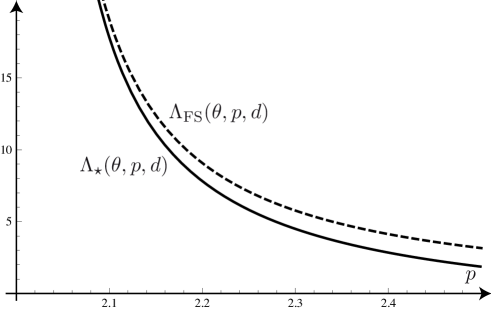
Figure 1: Curves $p\mapsto\Lambda_{\star}(\theta,p,d)$ and $\Lambda\mapsto\Lambda_{\rm FS}(\theta,p,d)$ with $\theta=0.5$ and $d=5$. Symmetry holds for $\Lambda\leq\Lambda_{\star}(\theta,p,d)$, while symmetry is broken for $\Lambda\geq\Lambda_{\rm FS}(\theta,p,d)$. The relative difference of $\Lambda_{1}$ and $\Lambda_{2}$, i.e., $\Lambda_{2}(\theta,p,d)/\Lambda_{1}(\theta,p,d)-1$, is below 4%. The estimate of Proposition 2 is such that $1-\Lambda_{2,\rm approx}(\theta,p,d)/\Lambda_{2}(\theta,p,d)$ is of the order of $5\times 10^{-3}$.

In Fig. 2, we consider the critical case $\theta=\vartheta(p,d)$. The plot corresponds to $d=5$ and all $p$ in the interval $(2,10/3)$. The exponent $\vartheta(p,d)$ is the one which enters in the Gagliardo-Nirenberg inequality

$$\|{u}\|_{\mathrm{L}^{p}({\mathbb{R}}^{d})}^{2}\leq\mathsf{C}_{\rm GN}(p,d)\,\|{\nabla u}\|_{\mathrm{L}^{2}({\mathbb{R}}^{d})}^{2\,\vartheta(p,d)}\,\|{u}\|_{\mathrm{L}^{2}({\mathbb{R}}^{d})}^{2\,(1-\vartheta(p,d))}\quad\forall\,u\in\mathrm{H}^{1}({\mathbb{R}}^{d})$$

on the Euclidean space ${\mathbb{R}}^{d}$, without weights. Here $\mathsf{C}_{\rm GN}(p,d)$ denotes the optimal constant and $p\in(2,\infty)$ if $d=1$ or $2$, $p\in(2,2^{*}]$ if $d\geq 3$. The optimizers are radially symmetry but not known explicitly.

It has been shown in (1005, , Theorem 1.4) that optimal functions for (1) exist if $\mathsf{C}_{\rm GN}(p,d)<\mathsf{C}_{\rm CKN}(\theta,p,a)$. On the other hand, optimal functions cannot be symmetric $\mathsf{C}_{\rm GN}(p,d)>\mathsf{C}_{\rm CKN}^{*}(\theta,p,a)$: see (springerlink:10.1007/s00526-011-0394-y, , Section 5) for further details and consequences. This symmetry breaking condition determines a curve $p\mapsto\Lambda_{\rm GN}(p,d)$ which has been computed numerically in 1008 ; Oslo : there are values of $p$ and $d$ for which the condition $\Lambda>\Lambda_{\rm GN}(p,d)$, which guarantees symmetry breaking (but not existence), is weaker than the condition $\Lambda>\Lambda_{\rm FS}(\theta,p,d)$, that is $\Lambda_{\rm GN}(p,d)<\Lambda_{\rm FS}(\theta,p,d)$. See Fig. 2. A rather complete scenario of explanations, based on numerical computations and some formal expansions, has been established in Freefem ; DE2012 . As it had to be expected, we numerically observe that $\Lambda_{\star}(\theta,p,d)\leq\min\{\Lambda_{\rm FS}(\theta,p,d),\Lambda_{\rm GN}(p,d)\}$ when $\theta=\vartheta(p,d)$, for any $p\in(2,2^{*})$.

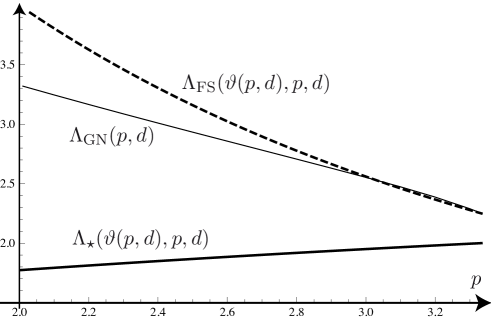
Figure 2: With $\theta=\vartheta(p,d)$, the curve $p\mapsto\Lambda_{\star}(\theta,p,d)$ is always below the curves $p\mapsto\Lambda_{\rm FS}(\theta,p,d)$ and $p\mapsto\Lambda_{\rm GN}(p,d)$ for any $p\in(2,2^{*})$, although $\Lambda_{\rm FS}$ and $\Lambda_{\rm GN}$ are not ordered. The plot corresponds to $d=5$ and we may notice that $\Lambda_{\rm GN}(p,d)<\Lambda_{\rm FS}$ if $p$ is small enough.

Acknowlegments. J.D. thanks S.F. and A.T. for welcoming him in Heraklion. J.D. and M.J.E. have been supported by the ANR project NoNAP. J.D. has also been supported by the ANR projects STAB and Kibord.
© 2014 by the authors. This paper may be reproduced, in its entirety, for non-commercial purposes.

References

- (1) M. Abramowitz and I. A. Stegun, Handbook of mathematical functions with formulas, graphs, and mathematical tables, vol. 55 of National Bureau of Standards Applied Mathematics Series, U.S. Government Printing Office, Washington, D.C., 1964.
- (2) L. Caffarelli, R. Kohn, and L. Nirenberg, First order interpolation inequalities with weights, Compositio Math., 53 (1984), pp. 259–275.
- (3) F. Catrina and Z.-Q. Wang, On the Caffarelli-Kohn-Nirenberg inequalities: sharp constants, existence (and nonexistence), and symmetry of extremal functions, Comm. Pure Appl. Math., 54 (2001), pp. 229–258.
- (4) M. del Pino, J. Dolbeault, S. Filippas, and A. Tertikas, A logarithmic Hardy inequality, J. Funct. Anal., 259 (2010), pp. 2045–2072.
- (5) J. Dolbeault, M. Esteban, G. Tarantello, and A. Tertikas, Radial symmetry and symmetry breaking for some interpolation inequalities, Calculus of Variations and Partial Differential Equations, 42 (2011), pp. 461–485.
- (6) J. Dolbeault and M. J. Esteban, Extremal functions in some interpolation inequalities: Symmetry, symmetry breaking and estimates of the best constants, Proceedings of the QMath11 Conference Mathematical Results in Quantum Physics, World Scientific, edited by Pavel Exner, 2011, pp. 178–182.
- (7) , About existence, symmetry and symmetry breaking for extremal functions of some interpolation functional inequalities, in Nonlinear Partial Differential Equations, H. Holden and K. H. Karlsen, eds., vol. 7 of Abel Symposia, Springer Berlin Heidelberg, 2012, pp. 117–130. 10.1007/978-3-642-25361-4-6.
- (8) J. Dolbeault and M. J. Esteban, Extremal functions for Caffarelli-Kohn-Nirenberg and logarithmic Hardy inequalities, Proceedings of the Royal Society of Edinburgh, Section: A Mathematics, 142 (2012), pp. 745–767.
- (9) J. Dolbeault and M. J. Esteban, A scenario for symmetry breaking in Caffarelli-Kohn-Nirenberg inequalities, Journal of Numerical Mathematics, 20 (2013), pp. 233—249.
- (10) , Branches of non-symmetric critical points and symmetry breaking in nonlinear elliptic partial differential equations, Nonlinearity, 27 (2014), p. 435.
- (11) J. Dolbeault, M. J. Esteban, A. Laptev, and M. Loss, One-dimensional Gagliardo–Nirenberg–Sobolev inequalities: remarks on duality and flows, Journal of the London Mathematical Society, (2014).
- (12) J. Dolbeault, M. J. Esteban, and M. Loss, Symmetry of extremals of functional inequalities via spectral estimates for linear operators, J. Math. Phys., 53 (2012), p. 095204.
- (13) J. Dolbeault, M. J. Esteban, M. Loss, and G. Tarantello, On the symmetry of extremals for the Caffarelli-Kohn-Nirenberg inequalities, Adv. Nonlinear Stud., 9 (2009), pp. 713–726.
- (14) J. Dolbeault, M. J. Esteban, and G. Tarantello, The role of Onofri type inequalities in the symmetry properties of extremals for Caffarelli-Kohn-Nirenberg inequalities, in two space dimensions, Ann. Sc. Norm. Super. Pisa Cl. Sci. (5), 7 (2008), pp. 313–341.
- (15) V. Felli and M. Schneider, Perturbation results of critical elliptic equations of Caffarelli-Kohn-Nirenberg type, J. Differential Equations, 191 (2003), pp. 121–142.