On the Reconstruction of Randomly Sampled Sparse Signals Using an Adaptive Gradient Algorithm

Abstract

Sparse signals can be recovered from a reduced set of samples by using compressive sensing algorithms. In common methods the signal is recovered in the sparse domain. A method for the reconstruction of sparse signal which reconstructs the remaining missing samples/measurements is recently proposed. The available samples are fixed, while the missing samples are considered as minimization variables. Recovery of missing samples/measurements is done using an adaptive gradient-based algorithm in the time domain. A new criterion for the parameter adaptation in this algorithm, based on the gradient direction angles, is proposed. It improves the algorithm computational efficiency. A theorem for the uniqueness of the recovered signal for given set of missing samples (reconstruction variables) is presented. The case when available samples are a random subset of a uniformly or nonuniformly sampled signal is considered in this paper. A recalculation procedure is used to reconstruct the nonuniformly sampled signal. The methods are illustrated on statistical examples.

1 Introduction

A discrete-time signal can be transformed into other domains in various ways. Some signals that cover whole considered interval in one domain could be sparse in a transformation domain. Compressive sensing theory, in general, deals with a lower dimensional set of linear observations of a sparse signal, in order to recover all signal values [1]-[26]. This area intensively develops in the last decade. A common form of observations are the signal samples. A reduced set of samples can be considered within the compressive sensing theory in order to represent a signal with the lowest possible number of samples. This theory may be applied to the situations when the missing samples are not a result of compressive sensing strategy, with the aim to reduce data size. In many engineering applications the signal samples are missing due to the system physical constraints or unavailability of the measurements. It can also happen that some arbitrarily positioned samples of a signal are so heavily corrupted by disturbances that it is better to omit them and consider as missing in the analysis [6], [28]. It is interesting to note that one of the first compressive sensing theory successes in applications (computed tomography reconstruction) was not related to the intentional compressive sensing strategy but to the physical problem constraints, restricting the set and positions of the available data. Signal reconstruction, with arbitrary missing samples, not being a result of any intentional compressive sensing strategy, is the topic of this paper.

Several approaches to reconstruct sparse signals from their random lower dimensional set of linear observations are introduced [8]-[19]. The most common are the reconstruction algorithms based either on the gradient formulations [8] or the orthogonal matching pursuit approaches [18].

Recently a method for the reconstruction of a sparse signal with disturbed/missing samples has been proposed [26]. In contrast to the common reconstruction methods that recover the signal in their sparsity domain the proposed method reconstructs missing samples/measurements to make the set of samples/measurements complete. Since the available samples are fixed, the minimization variables are the missing samples. It means that the number of variables is equal to the number of missing signal samples in the observation domain. A new criterion for the parameter adaptation of this simple algorithm, based on the gradient directions, is proposed in this paper. Computational time to achieve the target reconstruction accuracy is significantly reduced with respect to the original criterion in [26]. The Fourier transform domain is used as a case study, although the algorithm application is not restricted to this transform [27]. The algorithm efficiency is statistically checked. After the recovery of sparse signal, then its uniqueness is checked by using the proposed theorem. Its application is quite simple and numerically efficient.

Sparse signals with available samples being a random subset of nonuniformly sampled signal, not corresponding to the uniform sampling grid, are considered as well [29]-[33]. This case belongs to class of signals with indirect measurements. A possibility to recalculate the signal values at the sampling theorem positions is exploited in the nonuniform case before a reconstruction algorithm is applied [34].

The paper is organized as follows. After the definitions in the next section, the adaptive gradient algorithm, with a new criterion for the algorithm parameter adaptation, is presented in Section 3. Uniqueness of the obtained solution is analyzed in Section 3. Reconstruction of nonuniformly sampled sparse signals is considered in Section 4.

2 Gradient-based Reconstruction

Consider a discrete-time signal $x(n)$ with $N$ samples whose transform coefficients are $X(k)=T[x(n)]$. Signal $x(n)$ is sparse in the transformation domain if the number of nonzero transform coefficients $s$ is much lower than the number of the original signal samples $N$, $s\ll N$, i.e., $X(k)=0$ for $k\notin\{k_{1}$, $k_{2}$, …, $k_{s}\}$. The DFT will be considered in this paper, when $X(k)=\mathrm{DFT}[x(n)].$   Assume that a set of $M<N$ signal samples in the time domain is available at the instants corresponding to the discrete-time positions

$$n_{i}\in\mathbb{N}_{A}=\{n_{1},n_{2},...,n_{M}\}\subset\mathbb{N}=\{0,1,2,...,N-1\}.$$ (1)

In general, the signal recovery within the compressive sensing framework consists in reconstructing the signal (calculation of missing/unavailable/discarded samples) so that the number of nonzero transform coefficients $X(k)$ is minimal, subject to the available sample values. Counting of the nonzero transform coefficients is achieved by a simple mathematical form $\left\|X(k)\right\|_{0}$, sometimes referred to as the “$\ell_{0}$-norm”, [1], [24]. Thus, the problem statement is

$$\min\left\|X(k)\right\|_{0}\text{ subject to }\mathbf{y=AX},$$ (2)

where $\mathbf{y}=[x(n_{1})~{}~{}x(n_{2})~{}~{}...~{}~{}x(n_{M})]^{T}$ is the vector of available signal samples, $\mathbf{X}=[X(1)~{}~{}X(2)~{}~{}...~{}~{}X(N)]^{T}$ is the vector of unknown transform coefficients, and $\mathbf{A}$ is the inverse transform matrix with omitted rows corresponding to the unavailable signal samples. The $\ell_{0}$-norm based formulation is an NP-hard combinatorial optimization problem. Its calculation complexity is of order $\binom{N}{s}$. In theory, the NP-hard problems can be solved by an exhaustive search. However, as the problem parameters $N$ and $s$ increase the running time increases and the problem becomes unsolvable. These are the reasons why the $\ell_{1}$-norm of the signal transform, $\left\|X(k)\right\|_{1}=\sum_{k=0}^{N-1}\left|X(k)\right|$, is commonly used as a sparsity measure function. The minimization problem is

$$\min\sum_{k=0}^{N-1}\left|X(k)\right|\text{ subject to }\mathbf{y=AX.}$$ (3)

This minimization problem, under the conditions defined within the restricted isometry property (RIP), [3], [4], can produce the same result as (2).  Note that other norms $\ell_{p}$ between the $\ell_{0}$-norm and the $\ell_{1}$-norm, with values $0<p<1$, are also used in the minimization in attempts to combine good properties of these two norms [1, 26, 35].

2.1 Algorithm

A simple gradient-based algorithm that iteratively calculates the missing sample values according to (3), is presented next. The basic idea for the algorithm comes from the gradient-based minimization approaches. The missing samples are considered as variables. The influence of their variations on the sparsity measure is checked [26]. By performing an iterative procedure, the missing samples are changed toward lower sparsity measure values, in order to approach the minimum of the convex $\ell_{1}$-norm based sparsity measure (3). If the recovery conditions for the $\ell_{1}$-norm [3] are met then the $\ell_{1}$-norm minimum will be at the same position as the $\ell_{0}$-norm minimum, representing the true values of the missing samples.

2.2 Review of the Algorithm

The initial signal $y^{(0)}(n)$ is defined for $n\in$ $\mathbb{N}=\{0,1,\ldots,N-1\}$ as:

$$y^{(0)}(n)=\left\{\begin{array}[c]{ll}0&\text{ for missing samples, }n\in\mathbb{N}_{Q}\\ x(n)&\text{ for available samples, }n\in\mathbb{N}_{A}\end{array}\right.,$$ (4)

where $\mathbb{N}_{Q}$ is the complement of $\mathbb{N}_{A}$ with respect to $\mathbb{N}$ defined by (1).

The missing signal samples are then corrected in an iterative procedure as

$$y^{(m)}(n)=y^{(m-1)}(n)-g^{(m)}(n),$$ (5)

where $g^{(m)}(n)$ is an estimate of the sparsity measure gradient vector coordinate along the variable $y(n)$ direction, in the $m$th iteration. At the positions of the available signal samples, $n\in\mathbb{N}_{A}$, $g^{(m)}(n)=0$. At the positions of missing samples, $n_{i}\in\mathbb{{N}}_{Q}$, its values are calculated by changing the signal values and forming new signals $y_{1}(n)$ and $y_{2}(n)$ as

$$y_{1}(n) =y^{(m)}(n)+\Delta\delta(n-n_{i})$$

$$y_{2}(n) =y^{(m)}(n)-\Delta\delta(n-n_{i}).$$ (6)

The algorithm step is denoted by $\Delta$. The values of $g^{(m)}(n_{i})$ at $n_{i}\in\mathbb{N}_{Q}$ are

$$g(n_{i})=\frac{\sum_{k=0}^{N-1}\left|Y_{1}(k)\right|-\sum_{k=0}^{N-1}\left|Y_{2}(k)\right|}{N},$$ (7)

where $Y_{1}(k)=\mathrm{DFT}[y_{1}(n)]$ and $Y_{2}(k)=\mathrm{DFT}[y_{2}(n)]$.

The initial value for the algorithm adaptation step $\Delta$ is estimated as

$$\Delta=\max_{n\in\mathbb{N}_{A}}|x(n)|=\max_{n}\left|y^{(0)}(n)\right|.$$ (8)

The gradient algorithm will approach the minimum point of the $\ell_{1}$-norm based sparsity measure with a precision related to the algorithm step $\Delta$.

2.2.1 Stopping Criterion and Adaptive Step

Rate of the algorithm convergence for different steps is considered in [26]. The algorithm performance is significantly improved by using adaptive step $\Delta$. A criterion that efficiently detects the event that the algorithm has reached the vicinity of the sparsity measure minimum is proposed in this paper. It is based on the direction change of the gradient vector. When the vicinity of the optimal point is reached, the gradient estimate in the $\ell_{1}$-norm based sparsity measure function changes direction for almost $180$ degrees. For each two successive gradient estimations $g^{(m-1)}(n)$ and $g^{(m)}(n)$, the angle $\beta_{m}$ between gradient vectors is calculated as

$$\beta_{m}=\arccos\frac{\sum_{n=0}^{N-1}g^{(m-1)}(n)g^{(m)}(n)}{\sqrt{\sum_{n=0}^{N-1}\left(g^{(m-1)}(n)\right)^{2}}\sqrt{\sum_{n=0}^{N-1}\left(g^{(m)}(n)\right)^{2}}}.$$

If the angle $\beta_{m}$ is above $170^{\circ}$ it means that the values reached oscillatory nature around the minimal measure value position. When this kind of the angle change is detected the step $\Delta$ is reduced, for example, $\Delta/\sqrt{10}\rightarrow\Delta$, and the same calculation procedure is continued from the reached reconstructed signal values. When the optimal point is reached with a sufficiently small $\Delta$, then this value of $\Delta$ is also an indicator of the solution precision. Value of $\Delta$ can be used as the algorithm stopping criterion.

A common way to estimate the precision of the result in iterative algorithms is based on the change of the result in the last iteration. An average of changes in last iteration in a large number of missing samples is a good estimate of the achieved precision. Thus, the value of

$$T_{r}=10\log_{10}\frac{\sum_{n\in\mathbb{N}_{Q}}|y_{p}(n)-y^{(m)}(n)|^{2}}{\sum_{n\in\mathbb{N}_{Q}}|y^{(m)}(n)|^{2}}.$$

can be used as an rough estimate of the reconstruction error to signal ratio. Here $y_{p}(n)$ is the reconstructed signal prior to $\Delta$ reduction (prior to the execution of the algorithm inner loop, lines 7-20 in Algorithm 1) and $y^{(m)}(n)$ is the reconstructed signal after the inner loop execution. This value can also be used as a criterion to stop the algorithm. If $T_{r}$ is above the required precision threshold $T_{max}$ (for example, if $T_{r}>-100dB$), the calculation procedure should be repeated with smaller values $\Delta$.

A pseudo code of this algorithm is presented in Algorithm 1.

Algorithm 1 Reconstruction

1:

2:

• Set of missing/omitted sample positions $\mathbb{N}_{Q}$

• Available samples $x(n)$, $n\notin\mathbb{N}_{Q}$

3:

4:Set $y^{(0)}(n)\leftarrow x(n)$ $\triangleright$ for $n\notin\mathbb{N}_{Q}$

5:Set $y^{(0)}(n)\leftarrow 0$ $\triangleright$ for $n\in\mathbb{N}_{Q}$

6:Set $m\leftarrow 0$

7:Set $\Delta\leftarrow\max{|y^{(0)}(n)|}$

8:repeat

9:     Set $y_{p}(n)=y^{(m)}(n)$ $\triangleright$ for each $n$

10:     repeat

11:         $m\leftarrow m+1$

12:         for  $n_{i}\leftarrow 0$ to $N-1$ do

13:              if  $n_{i}\in\mathbb{N}_{Q}$ then

14:                  $Y_{1}(k)\leftarrow\operatorname*{DFT}\{y^{(m)}(n)+\Delta\delta(n-n_{i})\}$

15:                  $Y_{2}(k)\leftarrow\operatorname*{DFT}\{y^{(m)}(n)-\Delta\delta(n-n_{i})\}$

16:                  $\displaystyle g^{(m)}(n_{i})\leftarrow\frac{1}{N}{\sum_{k=0}^{N-1}|Y_{1}(k)|-|Y_{2}(k)|}$

17:              else

18:                  $g^{(m)}(n_{i})\leftarrow 0$

19:              end if

20:              $y^{(m+1)}(n_{i})\leftarrow y^{(m)}(n_{i})-g^{(m)}(n_{i})$

21:         end for

22:         $\displaystyle\beta_{m}=\arccos\frac{\sum_{n=0}^{N-1}g^{(m-1)}(n)g^{(m)}(n)}{\sqrt{\sum_{n=0}^{N-1}\left(g^{(m-1)}(n)\right)^{2}}\sqrt{\sum_{n=0}^{N-1}\left(g^{(m)}(n)\right)^{2}}}$

23:     until  $\beta_{m}<170^{\circ}$

24:     $\Delta\leftarrow\Delta/\sqrt{10}$

25:     $\displaystyle T_{r}=10\log_{10}\frac{\sum_{n\in\mathbb{N}_{Q}}|y_{p}(n)-y^{(m)}(n)|^{2}}{\sum_{n\in\mathbb{N}_{Q}}|y^{(m)}(n)|^{2}}.$

26:until  $T_{r}<T_{max}$

27:return $y^{(m)}(n)$

28:

29:

30:

• Reconstructed signal $x_{R}(n)=y^{(m)}(n)$

Comments on the algorithm:

- The inputs to the algorithm are the signal length $N$, the set of available samples $\mathbb{N}_{A}$, the available signal values $x(n_{i})$, $n_{i}\in$ $\mathbb{N}_{A}$, and the required precision $T_{max}$.

- Instead of calculating signals (6) and their $\mathrm{DFTs}$ for each $n_{i}\in\mathbb{N}_{Q}$ we can calculate

$$\left|Y_{1}(k)\right| =\left|Y^{(m)}(k)+\Delta D_{n_{i}}(k)\right|$$

$$\left|Y_{2}(k)\right| =\left|Y^{(m)}(k)-\Delta D_{n_{i}}(k)\right|$$

with $Y^{(m)}(k)=\mathrm{DFT}[y^{(m)}(n)]$ and $D_{n_{i}}(k)=\mathrm{DFT}[\delta(n-n_{i})]=\exp(-j2\pi n_{i}k/N)$, for each $n_{i}\in\mathbb{N}_{Q}$. Since $D_{n_{i}}(k)$ are independent of the iteration number $m$ they can be calculated only once, independently from the DFT of the signal.

- In a gradient-based algorithm, a possible divergence is related to the algorithm behavior for a large step $\Delta$. Small steps influence the rate of the algorithm approach to the solution only, with the assumption that it exists. Influence of small steps to the calculation complexity is considered in [26]. Here, we will examine the algorithm behavior for a large value of step $\Delta$. We can write

$$\left|Y_{1}(k)\right|-\left|Y_{2}(k)\right| =\left|Y^{(m)}(k)+\Delta D_{n_{i}}(k)\right|-\left|Y^{(m)}(k)-\Delta D_{n_{i}}(k)\right|$$

$$=\Delta\left|D_{n_{i}}(k)\right|\left(\left|1+\frac{Y^{(m)}(k)}{\Delta D_{n_{i}}(k)}\right|-\left|1-\frac{Y^{(m)}(k)}{\Delta D_{n_{i}}(k)}\right|\right).$$

Considering the complex number $a=Y^{(m)}(k)/(\Delta D_{n_{i}}(k)),$ with $|a|\ll 1$ for a large $\Delta$, from the problem geometry it is easy to show that the following bounds hold $0\leq\left||1+a|-|1-a|\right|\leq 2\left|a\right|$. Therefore,

$$0\leq\Big{|}\left|Y_{1}(k)\right|-\left|Y_{2}(k)\right|\Big{|}\leq 2\left|Y^{(m)}(k)\right|.$$

Lower limit $0$ is obtained if $a$ is imaginary-valued, while the upper limit $2\left|Y^{(m)}(k)\right|$ follows if $a$ is real-valued.

It means that the value of the finite difference $\left|Y_{1}(k)\right|-\left|Y_{2}(k)\right|,$ that is used to correct the missing signal samples, does not depend on the value of the step $\Delta$, if $\Delta$ is large. The missing signal values will be adapted for a value independent on $\Delta$ in that case. The values of missing samples will oscillate within the range of the original signal values of order $\left|Y^{(m)}(k)\right|/N$, until $\Delta$ is reduced in the iterations. Then the missing samples will start approaching to the position of the sparsity measure minimum. The initial values will be arbitrary changed within the signal amplitude order as far as $\Delta$ is too large. It will not influence further convergence of the algorithm, when the step $\Delta$ assumes appropriate values.

- Since two successive gradient vectors are required to calculate the gradient angle $\beta_{m}$, it is calculated starting from the second iteration for each $\Delta$.

- The algorithm output is the reconstructed signal $y(n)$, $n=0,1,\ldots,N-1$.

- Other signal transforms can be used instead of the DFT. The only requirement is that signal is sparse in that transform domain.

Example 1: Consider a signal

$$x(t)=\sum_{i=1}^{K}A_{i}\cos(2\pi tk_{i}/T+\varphi_{i}),$$ (9)

with $t=n\Delta t,$ $\Delta t=1$, and the total number of samples $N=T/\Delta t$. The sparsity parameter $s=2K$ is changed from $s=2$ to $s=N/2$. The amplitudes $A_{i}$, frequencies $k_{i}$, and phases $\varphi_{i}$ are taken randomly. Amplitude values are modeled as Gaussian random variables with variance $1,$ the frequency indices assume random numbers within $1\leq k_{i}\leq N-1$, and the phases assume uniform random values within $0\leq\phi_{i}\leq 2\pi$, in each realization. The reconstruction is performed by using $100$ realizations for each $s$ with random sets of missing $N-M$ samples in each realization. The simulations are done for $N=128$ and for $N=64$. The reconstructed signals $x_{R}(n)$ are obtained. The results are presented in Fig.1(a) and (b) in a form of the signal-to-reconstruction-error ratio (SRR) in [dB]

$$SRR=10\log\frac{\sum_{n=0}^{N-1}\left|x(n)\right|^{2}}{\sum_{n=0}^{N-1}\left|x(n)-x_{R}(n)\right|^{2}}.$$ (10)

Figure 1: Signal-to-reconstruction-error (SRR) obtained by using Algorithm 1, averaged over 100 realizations for various sparsity $s$ and number of available samples $M$: (a) The total number of samples is $N=128$. (b) The total number of samples is $N=64.$ (c) With a Gaussian noise in the input signal, $SNR=20$ [dB] and $N=64.$

It is important to note that the all signal samples are used in this error calculation. It means that possible nonunique solutions, satisfying the same set of available samples, are considered as the reconstructions with significant error since they significantly differ at the positions of missing/recovered samples. This kind of reconstruction and uniqueness analysis is exact. However, it can be used in simulations only since it requires the exact signal in all samples. A check of the solution uniqueness, using the missing sample positions only, will be discussed later.

Red colors indicate the region where the algorithm had fully recovered missing samples (compared to the original samples) in all realizations, while blue colors indicate the region where the algorithm could not recover missing samples in any realization. In the transition region for $M$ slightly greater than $2s$ we have cases when the signal recovery is not achieved and the cases of full signal recovery. A stopping criterion for the accuracy of $120$ [dB] is used. It corresponds to a precision in the recovered signal of the same order as in input samples, if they are acquired by a 20-bit A/D converter. The case with $N=64$ is repeated with an additive input Gaussian noise such that the input signal-to-noise ratio is $20$ [dB] in each realization Fig.1(c). The reconstruction error in this case is limited by the input signal-to-noise value.

The average reconstruction error in the noise-free cases is related to the number of the full recovery events. For $N=64$ the number of the full recovery events is checked and presented in Fig.2 (a),(b). The average number of the algorithm iterations to produce the required precision, as a function of the number of missing samples and signal sparsity $s$, is presented as well, Fig.2(c), along with the corresponding average computation time (in seconds) for the Windows PC with Intel Dual Core processor, Fig.2(d). The average computation time is proportional to the average number of iterations multiplied by the number of missing samples (variables) $Q=N-M$.

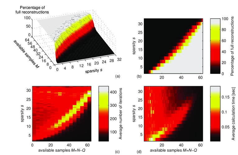
Figure 2: (a)-(b) The percentage of the full recovery events as a function of the number of available samples $M$ and the sparsity $s$ in the case of $N=64$. (c) The average number of iterations as a function of the number of missing samples and sparsity. (d) The average computation time.

Finite difference method and the adaptation procedure presented in this paper overcome the problem of the derivative existence in the case of the $\ell_{1}$-norm near the optimal point. Although the main point of this manuscript is to present a new method of reconstruction, with missing samples being minimization variables, efficiency of the presented algorithm is compared with the standard routines where the $\ell_{1}$-norm problem is solved using the linear programming. Direct adaptation of missing samples can be used in various applications (including recovery of sampled signals where a linear relation between signal and transform cannot be established). The performance of the proposed algorithm are compared with the algorithm that recasts the recovery problem (6) into a linear programming framework and uses the primal-dual interior point method (L1-magic code in MATLAB). Both algorithms are run with the default parameters using 100 sparse signals with random parameters. The results are presented in the Table 1. Columns notation in the table is: $s$ for sparsity, $Q=N-M$ for the number of missing samples, MAE stands for the mean absolute error, LP-DP denotes the values obtained by running the linear programming primal-dual algorithm (MATLAB L1-magic code), and AS is for the presented adaptive algorithm with variable step. Calculation time using MATLAB is presented in both cases.

Table 1: MAE and elapsed time for L1-magic (LP-DP) and proposed algorithm (AS)

$s$	$N-M$	MAE LP-DP	MAE AS	time LP-DP	time AS
6	16	$1.719\times 10^{-4}$	$3.959\times 10^{-7}$	0.043390	0.013433
10	16	$1.124\times 10^{-4}$	$3.730\times 10^{-7}$	0.041121	0.013393
16	16	$2.575\times 10^{-4}$	$5.943\times 10^{-7}$	0.041569	0.014003
6	32	$3.238\times 10^{-4}$	$8.000\times 10^{-7}$	0.038492	0.025733
10	32	$3.454\times 10^{-4}$	$1.133\times 10^{-6}$	0.038578	0.027270
16	32	$1.068\times 10^{-3}$	$1.818\times 10^{-6}$	0.046595	0.029636
6	45	$1.000\times 10^{-3}$	$1.295\times 10^{-6}$	0.041317	0.036442
10	45	$4.731\times 10^{-3}$	$1.878\times 10^{-6}$	0.039162	0.041843
16	45	$2.415\times 10^{-3}$	$2.751\times 10^{-6}$	0.042910	0.054350

An illustration of the algorithm performance regarding to the SRR and the gradient angle $\beta_{m}$ in one realization, with $s=6$, is presented in Fig.3.

Figure 3: Angle between successive gradient estimations $\beta_{m}$ and the signal-to-reconstruction-error ratio (SRR) as a function of the number of iterations in the algorithm for one signal realization with 6 nonzero DFT coefficients and $M=64$.

3 Uniqueness of the Obtained Solution

Uniqueness of the solution is guarantied if the restricted isometry property is used and checked, with appropriate isometry constant for the norm-one based minimization. However, two problem exist in the implementation of this method. For a specific measurement matrix it produces quite conservative bounds, meaning in practice a large number of false alarms for nonuniqueness. In addition the check of the restricted isometry property required a combinatorial approach, which is an NP hard problem (like the solution of the problem using zero-norm in minimization). The the gradient-based algorithm presented here considers missing samples/measurements as the minimization variables. A theorem for the solution uniqueness, in terms of the missing sample positions is used here. The proof of this theorem, with additional details and examples, is given in [36]. When the reconstruction of a signal is done and the solution of sparsity $s$ in the DFT domain is obtained, then the theorem provides an easy check for the solution uniqueness.

Consider a signal

$$x_{a}(n)=x(n)+z(n)$$

where $z(n)=0$ for $n\in\mathbb{M}$ and takes arbitrary values at the positions of missing samples $n=q_{m}\in\mathbb{N}_{Q}=\{q_{1},q_{2},....,q_{Q}\}$. The DFT of this signal is

$$X_{a}(k) =X(k)+Z(k)$$

$$=\sum_{i=1}^{s}\sigma_{i}\delta(k-k_{0i})+\sum_{m=1}^{Q}z(q_{m})e^{-j2\pi q_{m}k/N}.$$

The values of missing samples $y(n)=x_{a}(n)$ for $n\in\mathbb{N}_{Q}$ are considered as variables, in the sparsity measure minimization process, with the final goal to get $x_{a}(n)=x(n)$, or $z(n)=0$ for all $n$. Existence of unique solution depends on the number of missing samples $Q$, their positions $\mathbb{N}_{Q}$, and the available signal values [36]. The uniqueness here means that if a sparse signal, with the transform $X(k)$, is reconstructed using the fixed set of available samples and the gradient-based algorithm (or any other reconstruction algorithm), then there is no other signal transform of the same or lower sparsity satisfying the same set of available sample values.

Theorem.

Consider signal $x(n)$ that is sparse in the DFT domain with unknown sparsity. Assume that the signal length is $N=2^{r}$ samples and that $Q$ samples are missing at the instants $q_{m}\in\mathbb{N}_{Q}$. Also assume that the reconstruction is performed and that the DFT of reconstructed signal is of sparsity $s$. Assume that the positions of the reconstructed nonzero values in the DFT are $k_{0i}\in\mathbb{K}_{s}=\{k_{01},k_{02},....,k_{0s}\}.$ Reconstruction result is unique if the inequality

$$s<N-\max_{h=0,1,...,r-1}\left\{2^{h}\left(Q_{2^{h}}-1\right)-s+2S_{2^{r-h}}\right\}$$

holds. Integers $Q_{2^{h}}$ and $S_{2^{r-h}}$ are calculated as

$$Q_{2^{h}} =\max_{b=0,1,...,2^{h}-1}\{\operatorname{card}\{q:q\in\mathbb{N}_{Q}\text{ and }\operatorname{mod}(q,2^{h})=b\}\}$$

$$S_{2^{r-h}} =\sum_{l=1}^{Q_{2^{h}}-1}P_{h}(l)$$

$$P_{h}(l) =\underset{b=0,1,...,2^{r-h}-1}{\mathrm{sort}}\{\operatorname{card}\{k:k\in\mathbb{K}_{s}\text{ and }\operatorname{mod}(k,2^{r-h})=b\}\}$$

where $P_{h}(1)\leq P_{h}(2)\leq...\leq P_{h}(2^{r-h})$.

Signal independent uniqueness corresponds to the worst case signal form, when $S_{2^{r-h}}=0$.

The answer is obtained almost immediately, since the computational complexity of the Theorem is of order $O(N)$. The proof is given in [36].

4 Random Subset of Nonuniformly Sampled Values

Consider now a discrete-time signal obtained by sampling a continuous-time signal $x(t)$ at arbitrary positions. Since the DFT will be used in the analysis, we can assume that the continuous-time signal is periodically extended with a period $T$. According to the sampling theorem, the period $T$ is related to the number of samples $N$, the sampling interval $\Delta t$, and the maximal frequency $\Omega_{m}$ as $\Omega_{m}=\pi/\Delta t=\pi N/T$. The continuous-time signal can be written as an inverse Fourier series

$$x(t)=\sum_{k=-N/2}^{N/2-1}X_{k}e^{j2\pi kt/T},$$ (11)

with the Fourier series coefficients being related to the DFT as $X_{k}N=X(k)=\mathrm{DFT}[x(n)]$ and $x(n)=x(n\Delta t)$. The discrete-time index $n$ corresponds to the continuous-time instant $t=n\Delta t$. Discrete-frequency indices  are $k\in\{-N/2,...,-1,0,1,...,N/2-1\}$. Any signal value can be reconstructed from the samples taken according to the sampling theorem,

$$x(t)=\sum_{n=0}^{N-1}x(n\Delta t)e^{j(n-t/\Delta t)\pi/N}\frac{\sin[(n-\frac{t}{\Delta t})\pi]}{N\sin[(n-\frac{t}{\Delta t})\pi/N]}.$$ (12)

This relation holds for an even $N$, [34], [7].

A signal $x(t)$ is sparse in the transformation domain if the number of nonzero transform coefficients $s$ is much lower than the number of the original signal samples $N$ within $T$, $s\ll N$, i.e., $X_{k}=0$ for $k\notin\{k_{1}$, $k_{2}$, …, $k_{s}\}$. A signal

$$x(t)=\sum_{k\in\{k_{1},k_{2},...,k_{s}\}}X_{k}e^{j2\pi kt/T}.$$ (13)

of sparsity $s$ can be reconstructed from $M$ samples, where $M<N$, if the recovery conditions are met.

Consider now a random set of possible sampling instants $\{t_{1},t_{2},...,t_{N}\}$,

$$t_{i}=i\Delta t+\nu_{i},$$

where $\nu_{i}$ is a uniform random variable $-\Delta t/2\leq\nu_{i}\leq\Delta t/2$. Here $t_{i}$ denotes a time instant, while in the uniform sampling the discrete-time index $n_{i}$ has been used to indicate instant corresponding to $n_{i}\Delta t$. Assume that a random set of $M$ signal samples is available at

$$t_{i}\in\mathbb{T}_{A}=\{t_{1},t_{2},...,t_{M}\}.$$

Since the signal is available at randomly positioned instants the Fourier transform coefficients estimated as

$$\hat{X}_{k}=\sum_{t_{i}\in\mathbb{T}_{A}}x(t_{i})\exp(-j2\pi kt_{i}/T)$$

will not be sparse even if a large number $M$ of samples is available. To improve the results, the problem can be reformulated to produce a better estimation of the sparse signal transform during the recovery process. If the signal values were available at $t_{i}\in\mathbb{T}_{A}$ for $M=N$ the signal values at the sampling theorem positions could be recovered. The transformation matrix relating samples taken at $t_{i}$ with the signal values at the sampling theorem positions, according to (12), is

$$\left[\begin{array}[c]{c}x(t_{1})\\ x(t_{2})\\ ...\\ x(t_{N})\end{array}\right] =\left[\begin{array}[c]{cccc}b_{11}&b_{12}&...&b_{1N}\\ b_{21}&b_{22}&...&b_{2N}\\ ...&...&...&...\\ b_{N1}&b_{N2}&...&b_{NN}\end{array}\right]\left[\begin{array}[c]{c}x(1)\\ x(2)\\ ...\\ x(N)\end{array}\right]$$

$$\mathbf{\hat{x}} \mathbf{=Bx}$$

with

$$b_{ij}=\frac{\sin[(j-t_{i}/\Delta t)\pi]}{N\sin[(j-t_{i}/\Delta t)\pi/N]}e^{j(j-t_{i}/\Delta t)\pi/N}$$

A problem here is that we know just $M<N$ of signal samples. The values at unavailable positions $t_{i}\notin\mathbb{T}_{A}$ are assumed to be zero in the initial iteration. Their positions are assumed at the sampling theorem instants, $t_{i}=i\Delta t$ for $t_{i}\notin\mathbb{T}_{A}$, since they are not known anyway. With this assumption the problem reduces to the missing samples $q_{m}\in\mathbb{N}_{Q}=\{q_{1},q_{2},....,q_{Q}\}$, being  considered as variables and the remaining samples, defined by vector $\mathbf{x}$, being calculated as

$$\mathbf{x=B}^{-1}\mathbf{\hat{x}}.$$ (14)

The matrix $\mathbf{B}^{-1}$ is inverted only once for the given signal sample positions. There is a direct relation to calculate the values $x(n\Delta t)$ based on the randomly sampled values $x(t_{i})$, [34], where the inversion is not needed.

The algorithm is adapted to this kind of signals as follows:

The signals $\hat{y}_{1}(t_{i})=y^{(m)}(t_{i})+\Delta\delta(t-t_{i})$ and $\hat{y}_{2}(t_{i})=y^{(m)}(t_{i})-\Delta\delta(t-t_{i})$ are formed. The available samples are recalculated to $y_{1}(n)$ and $y_{2}(n)$ according to (14) as

$$\mathbf{y}_{1}\mathbf{=B}^{-1}\mathbf{\hat{y}}_{1}$$

and

$$\mathbf{y}_{2}\mathbf{=B}^{-1}\mathbf{\hat{y}}_{2}.$$

These signals are used in the next algorithm steps.

Example 2: Consider the signal defined by (9). Similar results for the SRR and the average number of iterations, for various $M$ and $s$, are obtained here as in Fig.1. Thus, they will not be repeated. Instead we will present a particular realization with $s=6$ nonzero DFT coefficients, out of $N=128$, and a number of available samples $M=16$ within the transition region, when the recovery is not always obtained. These realizations, when the recovery conditions, for a given signal and for some of the considered sets of available samples, are met, can still be detected. This process is especially important if we are not in the position to define the sampling strategy for $M=N-Q$ available samples in advance, like in the cases when the available samples are uncorrupted samples and their positions can be arbitrary. The criterion for detection of a sparse signal in recovery is the measure of the resulting signal sparsity. In this case measures closer to the $\ell_{0}$-norm should be used for a detection. For example, with $\ell_{1/4}$-form in the case of a false recovery all transform coefficients are nonzero with $\sum_{k=0}^{N-1}\left|X(k)/N\right|^{1/4}\sim N$. For a full recovery of a sparse signal the number of nonzero coefficients (the measure value) is much lower since $s\ll N$.

Consider the case with $M=16$ available randomly positioned samples and $s=6$ nonzero DFT coefficients. Among 100 performed realizations a possible sparse recovery event is detected (when the described sparsity measure of the result is much lower than $N$). The DFT coefficients set of the detected sparse signal is  $\mathbb{K}_{s}=\{22$, $35$, $59$, $69$, $93$, $106\}$. It confirms that the reconstructed signal is sparse. This sparse reconstruction is checked for uniqueness using the theorem. The missing samples are from the set $q_{m}\in\mathbb{N}_{Q}$. It is a set difference of all samples $\mathbb{N=}\left\{n\text{ \ }\left|0\leq n\leq 127\right.\right\}$ and

$$\mathbb{N}_{A}=\left\{7,\text{ }14,\text{ }18,\text{ }21,\text{ }34,\text{ }37,\text{ }51,\text{ }69,\text{ }79,\text{ }82,\text{ }89,\text{ }90,\text{ }99,\text{ }100\text{, }113,\text{ }117\right\}.$$

For $h=0,1,...,r-1=6$ corresponding values of $Q_{2^{h}}$ and $S_{2^{r-h}}$, defined in the theorem, are calculated. Their values are:

$$h$$

Note that $Q_{2^{0}}=112$ is the total number of missing samples, while $Q_{2^{1}}$ is obtained by counting odd and even samples in $\mathbb{N}_{Q}$ and taking higher number of these two. Since there are $54$ samples at odd positions and $58$ samples at even positions, it means that $Q_{2^{1}}=58$.

For $h=2$ there are $31$ missing sample $q_{m}\in\mathbb{N}_{Q}$ with $\mod(q_{m},4)=0$, $26$ missing samples with $\mod(q_{m},4)=1$, $27$ missing samples with $\mod(q_{m},4)=2$, and $28$ missing samples with $\mod(q_{m},4)=3,$ resulting in $Q_{2^{2}}=\max\{31,26,27,28\}=31$, and so on. We can easily conclude that samples $x(1)$ and $x(65)$ are missing, meaning that $Q_{64}$ assumes its maximal possible value $Q_{64}=2$.

Similar counting is done to get $S_{2^{7-h}}$. For example,

$$S_{2^{7-6}}=S_{2^{1}}=\sum_{l=1}^{Q_{64}-1}P_{6}(l)=\sum_{l=1}^{1}P_{6}(l)=P_{6}(1)$$

where array $P_{6}(l)$ is obtained by sorting number of even and odd elements in $\mathbb{K}_{s}$. Since there are $2$ even and $4$ odd elements $P_{6}(1)=2$ and $P_{6}(2)=4$ resulting in $S_{2^{1}}=2$.

As expected this set of $112$ missing samples $\mathbb{N}_{Q}$ does not guarantee a unique solution for an arbitrary signal of sparsity $s=6$. By using the theorem with $S_{2^{r-h}}=0$ and $Q_{2^{h}}$ presented in the previous table we easily get that the solution uniqueness for this set $\mathbb{N}_{Q}$ and arbitrary signal requires $s<4$. However, for the specific available signal values, a sparse signal is reconstructed in this case, with nonzero coefficients at $\mathbb{K}_{s}=\{22$, $35$, $59$, $69$, $93$, $106\}$. The uniqueness then means that starting from this signal we can not find another signal of the same sparsity by varying the missing signal samples positioned at $n\in\mathbb{N}_{Q}$. The theorem then gives the answer that this specific recovered signal $x_{R}(n)$, with specific missing sample values and positions $\mathbb{N}_{Q}$, is unique. It means that starting from $x_{R}(n)$ we can not get another signal of the same or lower sparsity by varying the missing samples only. The reconstructed signal is presented in Fig.4. The signal-to-reconstruction-error ratio defined by (10), calculated for all signal samples, is $SRR=111.08$ dB. It corresponds to the defined reconstruction algorithm precision of about $100$ dB.

Figure 4: Available randomly positioned samples $x(t_{i})$ (red dots) of a sparse signal $x(t)$ (top). Reconstructed signal $x_{R}(n)$ at the sampling theorem positions (blue dots) along with the available samples (red dots) (bottom). Continuous-time signal $x(t)$ is presented by solid line.

In addition to the considered case two obvious cases in the uniqueness analysis may appear: 1) when both, the reconstructed signal and the worst case analysis produce a unique solution using the set of missing samples $\mathbb{N}_{Q}$, and 2) when both of them produce a result stating that a signal with certain sparsity can not be reconstructed in a unique way with $\mathbb{N}_{Q}$. Finally, it is interesting to mention that there exists a fourth case when the set of missing samples can provide a unique reconstruction of sparse signal (satisfying unique reconstruction condition if it were possible to use $\ell_{0}$-norm in the minimization process), however the $\ell_{1}$-norm based minimization does not satisfy the additional restricted isometry property constraints [3], [4] to produce this solution (the same solution as the one which would be produced by the $\ell_{0}$-norm). This case will be detected in a correct way using the presented theorem. It will indicate that a unique solution is possible using $\mathbb{N}_{Q}$, while if the $\ell_{1}$-norm based minimization did not produce this solution as a result of the reconstruction algorithm, the specific reconstructed signal will not satisfy the uniqueness condition.

5 Conclusion

Analysis of nonuniformly sampled sparse signals is performed. A gradient-based algorithm with adaptive step is used for the reconstruction. A new criterion for the parameter adaptation in the algorithm, based on the gradient directions analysis, is proposed. It significantly improves the calculation efficiency of the algorithm.  The random nonuniformly positioned available samples are recalculated based on the sampling theorem reconstruction formula. Based on the new set of samples the recovery is performed. The methods are checked and illustrated on numerical examples.

6 References

References

- [1] D. L. Donoho, “Compressed sensing,” IEEE Trans. on Information Theory, vol. 52, no. 4, pp. 1289–1306, 2006.
- [2] E. J. Candès, J. Romberg, and T. Tao, “Robust uncertainty principles: Exact signal reconstruction from highly incomplete frequency information,” IEEE Trans. on Information Theory, vol. 52, no. 2, pp. 489–509, 2006.
- [3] E. J. Candès, “The restricted isometry property and its implications for compressed sensing”, Comptes Rendus Mathematique, vol. 346, no. 9, pp. 589-592, 2008.
- [4] D. Needell and J. A. Tropp, “CoSaMP: Iterative signal recovery from incomplete and inaccurate samples,” Applied and Computational Harmonic Analysis, vol. 20, no. 3, pp. 301–321,2009
- [5] L. Stanković, I. Orović, S. Stanković, and M. Amin, “Robust Time Frequency Analysis based on the L-estimation and Compressive Sensing,” IEEE Signal Processing Letters, vol. 20, no. 5, pp. 499–502, 2013.
- [6] R. E. Carrillo, K. E. Barner, and T. C. Aysal, “Robust sampling and reconstruction methods for sparse signals in the presence of impulsive noise,” IEEE Journal of Selected Topics in Signal Processing, 2010, vol. 4, no. 2, pp. 392–408.
- [7] L. Stanković, M. Daković, and T. Thayaparan, Time–Frequency Signal Analysis with Applications, Artech House, 2013.
- [8] M. A. Figueiredo, R. D. Nowak, and S. J. Wright, “Gradient projection for sparse reconstruction: Application to compressed sensing and other inverse problems,” IEEE Journal of Selected Topics in Signal Processing, vol. 1, no. 4, pp. 586–597, 2007.
- [9] S. Mallat, A Wavelet Tour of Signal Processing, Academic Press, San Diego, CA, 1998.
- [10] S. J. Wright, “Implementing proximal point methods for linear programming,” Journal of Optimization Theory and Applications, vol. 65, pp. 531–554, 1990.
- [11] T. Serafini, G. Zanghirati and L. Zanni, “Gradient projection methods for large quadratic programs and applications in training support vector machines,” Optimization Methods and Software, vol. 20, no. 2–3, pp. 353–378, 2004.
- [12] E. Candes, J. Romberg and T. Tao, “Robust uncertainty principles: Exact signal reconstruction from highly incomplete frequency information,” IEEE Trans. on Information Theory, vol. 52, pp. 489–509, 2006.
- [13] J. More and G. Toraldo, “On the solution of large quadratic programming problems with bound constraints,” SIAM Journal on Optimization, vol. 1, pp. 93–113, 1991.
- [14] G. Davis, S. Mallat and M. Avellaneda, “Greedy adaptive approximation,” Journal of Constructive Approximation, vol. 12, pp. 57–98, 1997.
- [15] D. Donoho, M. Elad, and V. Temlyakov, “Stable recovery of sparse overcomplete representations in the presence of noise,” IEEE Trans. on Information Theory, vol. 52, pp. 6–18, 2006.
- [16] B. Turlach, “On algorithms for solving least squares problems under an L1 penalty or an L1 constraint,” Proc. of the American Statistical Association; Statistical Computing Section, pp. 2572–2577, Alexandria, VA, 2005.
- [17] R. Baraniuk, “Compressive sensing,” IEEE Signal Processing Magazine, vol. 24, no. 4, 2007, pp. 118–121.
- [18] S. G. Mallat and Z. Zhang, “Matching pursuits with time-frequency dictionaries,” Signal Processing, IEEE Transactions on, vol. 41, no. 12, pp. 3397–3415, 1993.
- [19] I. Daubechies, M. Defrise, and C. De Mol, “An iterative thresholding algorithm for linear inverse problems with a sparsity constraint,” Communications on pure and applied mathematics, vol. 57, no. 11, pp. 1413–1457, 2004.
- [20] P. Flandrin and P. Borgnat, “Time-Frequency Energy Distributions Meet Compressed Sensing,” IEEE Trans. on Signal Processing, vol. 58, no. 6, 2010, pp. 2974–2982.
- [21] Y. D. Zhang and M. G. Amin, “Compressive sensing in nonstationary array processing using bilinear transforms,” in Proc. IEEE Sensor Array and Multichannel Signal Processing Workshop, Hoboken, NJ, June 2012.
- [22] L. Stanković, S. Stanković, and M. G. Amin, “Missing Samples Analysis in Signals for Applications to L-Estimation and Compressive Sensing,” Signal Processing, Elsevier, vol. 94, Jan. 2014, pp. 401–408.
- [23] S. Aviyente, “Compressed Sensing Framework for EEG Compression,” in Proc. Stat. Sig. Processing, 2007, Aug. 2007.
- [24] L. Stanković, “A measure of some time–frequency distributions concentration,” Signal Processing, vol. 81, pp. 621–631, 2001
- [25] E. Sejdić, A. Cam, L. F. Chaparro, C. M. Steele, and T. Chau, “Compressive sampling of swallowing accelerometry signals using TF dictionaries based on modulated discrete prolate spheroidal sequences,” EURASIP Journal on Advances in Signal Processing, 2012:101 doi:10.1186/1687–6180–2012–101.
- [26] L. Stanković, M. Daković and S. Vujović, “Adaptive Variable Step Algorithm for Missing Samples Recovery in Sparse Signals,” IET Signal Processing, vol. 8, no. 3, pp. 246 -256, 2014, (arXiv:1309.5749v1).
- [27] I. Stanković, Recovery of Images with Missing Pixels using a Gradient Compressive Sensing Algorithm, http://arxiv.org/ftp/arxiv/papers/1407/1407.3695.pdf, June 2014.
- [28] L. Stanković, M. Daković, and S. Vujović, “Reconstruction of Sparse Signals in Impulsive Noise,” IEEE Trans. on Signal Processing, submitted.
- [29] M. Wakin, S. Becker, E. Nakamura, M. Grant, E. Sovero, D. Ching, Y. Juhwan, J. Romberg, A. Emami-Neyestanak, E. Candes, ”A Nonuniform Sampler for Wideband Spectrally-Sparse Environments,” Emerging and Selected Topics in Circuits and Systems, IEEE Journal on, vol.2, no.3, pp.516,529, Sept. 2012.
- [30] M. Mishali,Y.C. Eldar, ”From Theory to Practice: Sub-Nyquist Sampling of Sparse Wideband Analog Signals,” Selected Topics in Signal Processing, IEEE Journal of, vol.4, no.2, pp.375,391, April 2010.
- [31] R. Grigoryan, T. L. Jensen, T. Arildsen, T. Larsen, ”Reducing the computational complexity of reconstruction in compressed sensing nonuniform sampling,” in Proceedings of the 21st EUSIPCO 2013, Sept. 2013.
- [32] J. A. Tropp, J.N. Laska, M.F. Duarte, J.K. Romberg, R.G. Baraniuk, ”Beyond Nyquist: Efficient Sampling of Sparse Bandlimited Signals,” Information Theory, IEEE Transactions on, vol.56, no.1, pp.520,544, Jan. 2010.
- [33] L. Chenchi, J.H. McClellan, ”Discrete random sampling theory,” Acoustics, Speech and Signal Processing (ICASSP), 2013 IEEE International Conference on, pp.5430-5434, May 2013.
- [34] E. Margolis and Y.C. Eldar, “Nonuniform Sampling of Periodic Bandlimited Signals,” IEEE Trans. on Signal Processing, vol. 56, no. 7, pp. 2728–2745, 2008.
- [35] H. Tsutsu, Y. Morikawa, ”An lp Norm Minimization Using Auxiliary Function for Compressed Sensing”, in Proc. IMECS, March 2012, Hong Kong.
- [36] L. Stanković, M. Daković, ”On the Uniqueness of the Sparse Signals Reconstruction Based on the Missing Samples Variation Analysis”, Signal Processing, submitted (simultaneously with this paper, can be considered as its second part).