Linear stability analysis of Poiseuille flow in porous medium with small suction and injection

Abstract

We investigate the effect of small suction Reynolds number and permeability parameter on the stability of Poiseuille fluid flow in a porous medium between two parallel horizontal stationary porous plates . We have shown that the perturbed flow is governed by an equation named modified Orr-Sommerfeld equation. We find also that the normalization of the wall-normal velocity with characteristic small suction (or small injection) velocity is important for a perfect command of porous medium fluid flow stability analysis. The stabilizing effect of the parameters in general and small suction Reynolds number and permeability parameters in particular on the linear stability are found.

Institut de Mathématiques et de Sciences Physiques, BP: 613 Porto Novo, Bénin

1 Introduction

The flows through porous medium are very much prevalent in nature and therefore, the study of such flows has become of principal interest in many scientific and engineering applications [1, 2, 3, 4, 5, 6, 7, 8, 9, 10, 11, 12, 13]. This type of flows has shown their great importance in petroleum engineering to study the movements of natural gas, oil and water through the oil reservoirs; in chemical engineering for the filtration and water purification processes. Further, to study the underground water resources and seepage of water in river beds one need the knowledge of the fluid flow through porous medium. Therefore, there are number of practical uses of the fluid flow through porous media. The porous medium is in fact a non-homogeneous medium but for the sake of analysis, it may be possible to replace it with a homogeneous fluid which has dynamical properties equal to those of non-homogeneous continuum. Thus one can study the flow of hypothetical fluid under the action of the properly averaged external flow and the complicated problem of the flow through a porous medium reduces to the flow problem of homogeneous fluid with some additional resistance[1]. In this work, we considered incompressible viscous fluid flow in porous medium between two porous plates. We assumed that the plates are parallel, horizontal and stationary. We applied injection at the lower plate and suction at upper see (Hinvi et al.[2]).

The objective is to study the effect of Reynolds number $R_{e\omega}$ and permeability parameter $Kp$ introduced in Navier-Stokes equations by the small suction velocity and permeability of medium, on the stability of the Poiseuille flow in porous medium as in (Hinvi et al.([2]and [4]) ). For this as in previous paper, we derive fourth-order equations named modified fourth-order Orr-Sommerfeld equations governing the stability analysis of Poiseuille flow in porous medium. This allowed us to see the simultanous effect of $V^{*}_{\omega}$ or $R_{e\omega}$ and medium permeability parameter $Kp$ on the stability in the boundary layer. Thus, we solve numerically the corresponding eigenvalues problems. We employ Matlab in all our numerical computations to find eigenvalues. Such attempt has been made earlier by Monwanou et al. [5] the case of the non-porous plate boundary layers (a flat plate-law) without wall suction by normalizing all the components of the velocity with the free stream velocity $U^{*}$.

The paper is organized as follows. In the second section the mathematical formulation of the problem is made. In the third section the modified Orr-Sommerfeld equation governing the stability analysis of Poiseuille flow in porous medium is deduced. In the fourth section, the effects of small injection/suction parameter $R_{e\omega}$, wave number $k$ and permeability parameter $K_{p}$ on linear stability of Poiseuille flow in porous medium will be investigated with the help of figures. The conclusions will be presented in the final section.

2 Mathematical formulation of the problem

We considered a Poiseuille viscous incompressible fluid flow between a porous me-dium. We assumed the medium isotrope see figure 1. The two porous parallel plates delimiters are assumed of infinite lengh, distant $h$. The $y^{*}$ axis is normal to the planes of the plates. We considered the simple case where, the permeability parameter $Kp$ and velocities suction and injection are constants. We work at constant temperature, the heat transfer aspect of the flow is not studied. The small constant injection $V_{\omega}$ is applied at the lower plate and a same small constant suction $V_{\omega}$, at the upper plate. The two plates are fixed. We choose the origine on the plane $(x^{*},0,z^{*})$ such as $-{h}\leq y^{*}\leq{h}$ and $x^{*}$ parallel to the direction of the mean fluid flow. Initially, $t^{*}<0$, the fluid is assumed to be at rest. When $t^{*}>0$, the fluid starts moving.

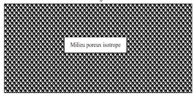
Figure 1: Porous medium.

The porous medium is infact a non-homogeneous medium but for the sake of analysis, it may be possible to replace it with a homogeneous continuum. Thus, one can study the flow of hypothetical homogeneous fluid under the action of the properly averaged external forces. Thus , a complicated problem of the flow through a porous medium reduces to the flow problem of a homogeneous fluid with some resistance. Then the equations of fluid flow in porous medium are simply the equations of fluid flow in homogeneous medium see (2) added the permeability term. Extra force terms as compared to non-porous medium fluid are added on $RHS$ of Navie-Stokes equations for homogeneous medium, due to the permeability medium. We can treat porous medium fluid as a single fluid under assumption that there is a permeability term to added.

Figure 2: Poiseuille porous parallel flat plates flow.

The equations of continuity, motion for the viscous incompressible fluid in porous medium are

$$\frac{\partial{\tilde{u}_{i}^{*}}}{\partial{\tilde{x}_{i}^{*}}} = 0,$$ (1)

$$\frac{\partial{\tilde{u}_{i}^{*}}}{\partial{\tilde{t}^{*}}}+\tilde{u}_{j}^{*}\frac{\partial{\tilde{u}_{i}^{*}}}{\partial{\tilde{x}_{j}^{*}}} = -\frac{1}{\rho}\frac{\partial{\tilde{p}}^{*}}{\partial{\tilde{x}_{i}^{*}}}+{\nu}\frac{\partial^{2}{\tilde{u}_{i}^{*}}}{{\partial{\tilde{x}_{j}^{*}}}^{2}}-\frac{\mu\tilde{u}_{i}^{*}}{\rho k^{*}}.$$ (2)

We introduced the following non-dimensional quantities as in (Hinvi et al.([2])

$$\tilde{x}=\frac{x^{*}}{h},\qquad\tilde{y}=\frac{y^{*}}{h},\qquad\tilde{z}=\frac{z^{*}}{h},$$

$$\tilde{u}=\frac{u^{*}}{U},\qquad\tilde{v}=\frac{v^{*}}{V_{\omega}},\qquad\tilde{w}=\frac{w^{*}}{U},$$

$$\tilde{t}=\frac{Ut^{*}}{h},\qquad\tilde{w}=\frac{w^{*}}{U},\qquad\tilde{p}=\frac{p^{*}}{\rho U^{2}},$$

$$R_{e}=\frac{Uh}{\nu},\qquad R_{e\omega}=\frac{V_{\omega}h}{\nu},\qquad K_{p}=\frac{k^{*}}{h^{2}}$$

Then the Eqs.(1) and (2) become in cartesien cordinates:

$$\frac{\partial{\tilde{u}}}{\partial{\tilde{x}}}+\frac{R_{e\omega}}{R_{e}}\frac{\partial{\tilde{v}}}{\partial{{\tilde{y}}}}+\frac{\partial{\tilde{w}}}{\partial{\tilde{z}}} = 0$$ (3)

$$\frac{\partial{\tilde{u}}}{\partial{\tilde{t}}}+\tilde{u}\frac{\partial{\tilde{u}}}{\partial{\tilde{x}}}+\frac{R_{e\omega}}{R_{e}}\tilde{v}\frac{\partial{\tilde{u}}}{\partial{\tilde{y}}}+\tilde{w}\frac{\partial{\tilde{u}}}{\partial{\tilde{z}}} = -\frac{\partial{\tilde{p}}}{\partial{\tilde{x}}}+\frac{{\triangledown}^{2}\tilde{u}}{R_{e}}-\frac{\tilde{u}}{K_{p}R_{e}},$$ (4)

$$\frac{\partial{\tilde{v}}}{\partial{\tilde{t}}}+\tilde{u}\frac{\partial{\tilde{v}}}{\partial{\tilde{x}}}+\frac{R_{e\omega}}{R_{e}}\tilde{v}\frac{\partial{\tilde{v}}}{\partial{\tilde{y}}}+\tilde{w}\frac{\partial{\tilde{v}}}{\partial{\tilde{z}}} = -\frac{R_{e}}{R_{e\omega}}\frac{\partial{\tilde{p}}}{\partial{\tilde{y}}}+\frac{{\triangledown}^{2}\tilde{v}}{R_{e}}-\frac{\tilde{v}}{K_{p}R_{e}},$$ (5)

$$\frac{\partial{\tilde{w}}}{\partial{\tilde{t}}}+\tilde{u}\frac{\partial{\tilde{w}}}{\partial{\tilde{x}}}+\frac{R_{e\omega}}{R_{e}}\tilde{v}\frac{\partial{\tilde{w}}}{\partial{\tilde{y}}}+\tilde{w}\frac{\partial{\tilde{w}}}{\partial{\tilde{z}}} = -\frac{\partial{\tilde{p}}}{\partial{\tilde{z}}}+\frac{{\triangledown}^{2}\tilde{w}}{R_{e}}-\frac{\tilde{w}}{K_{p}R_{e}}.$$ (6)

3 The linear disturbance equations

The flow is decomposed into the mean flow and the deviation from it (the disturbance) according to

$$\tilde{u}_{i}(r,t) = U_{i}(r)+u_{i}(r,t),$$ (7)

$$\tilde{p}(r,t) = P(r)+p(r,t).$$ (8)

where $r=(x,y,z)$ is the spatial coordinate vector.

Inserting (7) and (8) into the Navier-Stokes equations (3)- (6) we obtain the equations following.

$$\frac{\partial{u}}{\partial{t}}+U\frac{\partial{u}}{\partial{x}}+u\frac{\partial{U}}{\partial{x}}+\frac{R_{e\omega}V}{R_{e}}\frac{\partial{u}}{\partial{y}}+\frac{R_{e\omega}v}{R_{e}}\frac{\partial{U}}{\partial{y}}+{{W}}\frac{\partial{{u}}}{\partial{{z}}}+{{w}}\frac{\partial{{U}}}{\partial{{z}}} =$$

$$-\frac{\partial{p}}{\partial{x}}+\frac{{\triangledown}^{2}u}{R_{e}}-\frac{{u}}{K_{p}R_{e}},$$ (9)

$$\frac{\partial{v}}{\partial{t}}+U\frac{\partial{v}}{\partial{x}}+u\frac{\partial{V}}{\partial{x}}+\frac{R_{e\omega}V}{R_{e}}\frac{\partial{v}}{\partial{y}}+\frac{R_{e\omega}v}{R_{e}}\frac{\partial{V}}{\partial{y}}+{W}\frac{\partial{{v}}}{\partial{{z}}}+{{w}}\frac{\partial{{V}}}{\partial{{z}}} =$$

$$-\frac{\partial{p}}{\partial{y}}+\frac{{\triangledown}^{2}v}{R_{e}}-\frac{{v}}{K_{p}R_{e}},$$ (10)

$$\frac{\partial{w}}{\partial{t}}+U\frac{\partial{w}}{\partial{x}}+u\frac{\partial{W}}{\partial{x}}+\frac{R_{e\omega}V}{R_{e}}\frac{\partial{w}}{\partial{y}}+\frac{R_{e\omega}v}{R_{e}}\frac{\partial{W}}{\partial{y}}+{{W}}\frac{\partial{{w}}}{\partial{{z}}}+{{w}}\frac{\partial{{W}}}{\partial{{z}}} =$$

$$-\frac{\partial{p}}{\partial{z}}+\frac{{\triangledown}^{2}w}{R_{e}}-\frac{{w}}{K_{p}R_{e}},$$ (11)

$$\frac{\partial{{u}}}{\partial{{x}}}+\frac{R_{e\omega}}{R_{e}}\frac{\partial{{v}}}{\partial{{y}}}+\frac{\partial{{w}}}{\partial{{z}}} = 0.$$ (12)

We take the dimensional base flow for small suction and injection see (Hinvi et al.[2]):

$$U(y) = (1-y^{2})$$ (13)

$$V = 1$$ (14)

$$W = 0.$$ (15)

To obtain the stability equations for the spatial evolution of three-dimensional, we take the dependent on time disturbances

$$(u(x,y,z,t);v(x,y,z,t);w(x,y,z,t);p(x,y,z,t));$$ (16)

which are scaled in the same way as above.

With the equations (13-16), the equations (9-12) become

$$\frac{\partial{u}}{\partial{t}}+U\frac{\partial{u}}{\partial{x}}+\frac{R_{e\omega}}{R_{e}}\frac{\partial{u}}{\partial{y}}+\frac{R_{e\omega}}{R_{e}}v\frac{\partial{U}}{\partial{y}} = -\frac{\partial{p}}{\partial{x}}+\frac{{\triangledown}^{2}u}{R_{e}}-\frac{{u}}{K_{p}R_{e}},$$ (17)

$$\frac{\partial{v}}{\partial{t}}+U\frac{\partial{v}}{\partial{x}}+\frac{R_{e\omega}}{R_{e}}\frac{\partial{v}}{\partial{y}} = -\frac{R_{e}}{R_{e\omega}}\frac{\partial{p}}{\partial{y}}+\frac{{\triangledown}^{2}v}{R_{e}}-\frac{{v}}{K_{p}R_{e}},$$ (18)

$$\frac{\partial{w}}{\partial{t}}+U\frac{\partial{w}}{\partial{x}}+\frac{R_{e\omega}}{R_{e}}\frac{\partial{w}}{\partial{y}} = -\frac{\partial{p}}{\partial{z}}+\frac{{\triangledown}^{2}w}{R_{e}}-\frac{{w}}{K_{p}R_{e}}.$$ (19)

$$\frac{\partial{u}}{\partial{x}}+\frac{R_{e\omega}}{R_{e}}\frac{\partial{v}}{\partial{y}}+\frac{\partial{w}}{\partial{z}} = 0.$$ (20)

The equations (17-20) above are the linear disturbance equations that model the Poi-seuille flow of the incompressible viscous fluid in porous medium with the assumption that there is a constant small suction at upper plate and a constant small injection at the lower plate in cartesien coordinates.

4 Modified Orr-Sommerfeld equation

In this section the modified Orr-Sommerfeld equation governing the stability analysis of Poiseuille flow in porous medium is deduced by using Navier-Stokes equations with the same strategy as ( see Hinvi et al.[2]). By using continuity equation, the pressure terms can be eliminated from (17)-(20), by reducing the system to two equations for two unknown quantities. For a mean profile (13-15), the divergence of (17)-(20) and continuity gives

$${\bigtriangledown}^{2}{p} = -2\frac{R_{e\omega}}{R_{e}}\frac{\partial{U}}{\partial{y}}\frac{\partial{v}}{\partial{x}}.$$ (21)

We applied $\bigtriangledown^{2}$ to the equation (18), unsing (21) we found

$$\frac{\partial{}}{\partial{t}}{\bigtriangledown}^{2}{v}+{U}\frac{\partial{}}{\partial{x}}{\bigtriangledown}^{2}{v}+\frac{R_{e\omega}}{R_{e}}\frac{\partial{}}{\partial{y}}{\bigtriangledown}^{2}{v}-\frac{d^{2}U}{{dy}^{2}}\frac{\partial{v}}{\partial{x}}-2\frac{dU}{{dy}}\frac{\partial^{2}{v}}{\partial{x}\partial{y}} =$$

$$\frac{1}{R_{e}}{\bigtriangledown}^{4}{v}-\frac{\bigtriangledown^{2}v}{K_{p}R_{e}}.$$ (22)

By neglecting the quadratic derivation (because of linear stability analysis) the equation (22) becomes

$$\left(\frac{\partial{}}{\partial{t}}+{U}\frac{\partial{}}{\partial{x}}+\frac{1}{K_{p}R_{e}}+\frac{R_{e\omega}}{R_{e}}\frac{\partial{}}{\partial{y}}\right){\bigtriangledown}^{2}{v}-\frac{d^{2}U}{{dy}^{2}}\frac{\partial{v}}{\partial{x}} = \frac{1}{R_{e}}{\bigtriangledown}^{4}{v}.$$

We transform the Eq.(22) in an eigenvalue problem. Thus, the disturbances are taken to be periodic in time in the streamwise, spanwise directions, which allow us to assume solutions of the form

$$f(x,y,z,t) = \hat{f}(y)e^{i(\alpha x+\beta z-\omega t)};$$ (23)

where $f$ represents either one of the disturbances $u$, $v$, $w$ or $p$ and $\hat{f}$ the amplitude function, $k$, $\alpha=k_{x}=k\cos{\theta}$ and $\beta=k_{z}=k\sin{\theta}$ are the wave numbers, $\omega=\alpha c$ is the frequency of the wave. With $i^{2}=-1$, $\theta=(\vec{k_{x}},\vec{k})$, $c=c_{r}+ic_{i}$ wave velocity which is taken to be complex, $\alpha$ and $\beta$ are real because of temporal stability analysis considered.

Then with the equation (23) the equation (4) becomes

$$i\alpha\left(U-c-i\frac{R_{e\omega}D}{{\alpha}R_{e}}-\frac{i}{{\alpha}K_{p}R_{e}}+i\frac{D^{2}-{k}^{2}}{\alpha R_{e}}\right)\left(D^{2}-{k}^{2}\right)\hat{v} =$$

$$-i\alpha U^{\prime\prime}\hat{v};$$ (24)

where $D=\frac{d}{dy}$.

We have a same boundary conditions $\hat{v}(\pm 1)=1,\qquad\hat{v}^{\prime}(\pm 1)=0$ as in (Hinvi et al.[2]).

To transform these boundary conditions to $\hat{v}_{p}(\pm 1)=\hat{v}_{p}^{\prime}(\pm 1)$ we make the change, by puting

$$v_{p}(x,y,z,t) = v(x,y,z,t)-1.$$ (25)

The equation (24) becomes then

$$\left[\left(U-i\frac{{{R_{e\omega}}}D}{{\alpha}R_{e}}-\frac{i}{{\alpha}{{K_{p}}}R_{e}}+i\frac{D^{2}-{k}^{2}}{\alpha R_{e}}\right)\left(D^{2}-{k}^{2}\right)-\left(U^{\prime\prime}\right)\right]\hat{v}_{p} =$$

$$c\left(D^{2}-k^{2}\right)\hat{v}_{p}$$ (26)

with boundary conditions for all $(x,\pm 1,z,t>0)$ :

$$\hat{v}_{p}(\pm 1)=\hat{v}_{p}^{\prime}(\pm 1)=0.$$ (27)

The Eq.(26) is a flow equation modified by suction Reynolds number ${R_{e\omega}}$ (or the speed of suction and injection) and permeability parameter $K_{p}$, which differentiated it, from the model study by (Hinvi et al.[2]) by permeability term, rewritten as an eigenvalue problem, where $c$ is the eigenvalue and $\hat{v}_{p}$ the eigenfunction.

$$\left(U-i\frac{{{R_{e\omega}}}D}{{\alpha}R_{e}}-\frac{i}{{\alpha}{{K_{p}}}R_{e}}+i\frac{D^{2}-{k}^{2}}{\alpha R_{e}}\right)\left(D^{2}-{k}^{2}\right)-\left(U^{\prime\prime}\right)$$

and $\left(D^{2}-k^{2}\right)$ are the operators.

5 Stability analysis

We consider three-dimensional disturbances. We use a temporal stability analysis as mentioned above. With $c$ complex as we have defined above, when $c_{i}<0$ we have stability, $c_{i}=0$ we have neutral stability and elsewhere we have instability. We employ Matlab $7.0$ in all our numerical computations to find the eigenvalues. The mean flow profile for Poiseuille flow in porous medium is

$$U=\left(1-y^{2},1,0\right)$$ (28)

for $R_{e\omega}$ small (i.e. small suction) is considered (see [3]) The eigenvalue problem (26)-27) is solved numerically with the suitable boundary conditions. The solutions are found in a layer bounded at $y=\pm 1$. The results of calculations are presented in the figures below. We present the figures related to the eigenvalue problem. For all figure we ploted $c_{i}=c_{i}(\mbox{one parameter)}$ by fixing the other parameters. The yellow color is for $c_{i}=0$.

Figure 3: Growth rate $c_{i}$ vs. Reynolds’ number for $k=1.02$, $R_{ew}=0$, $\theta=0\pi$, $Kp=0.045,0.048,0.13$ and $1$.

In the figure 3, we note for all small values of permeability parameter that, $ci>0$. We conclude that the flow is unstable anywhere. These curves also tell us that an increase in the permeability parameter promotes flow stability.

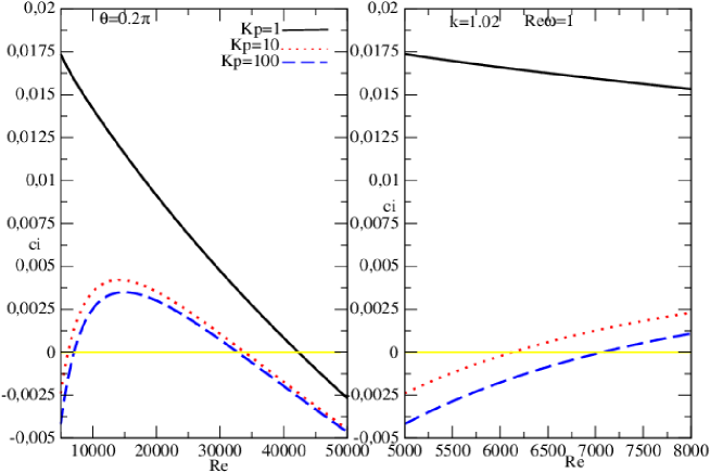
Figure 4: Growth rate $c_{i}$ vs. Reynolds’ number $R_{e}$, for $k=1.02$, $R_{ew}=1$, $\theta=0.2\pi$, $Kp=1,10,100$. The right frame is zoom of the left frame.

Through the curves of the figure 4, we remark that for $R_{e}\leq 6200$, large values of $Kp$ stabilize the flow and for the small value $Kp=1$ the flow is unstable. When $6200<R_{e}<33000$ for the all values of $Kp$ the flow is unstable and after ($R_{e}>33000$) it becomes stable elsewhere. The flow stabilizes for small values of $R_{e}$, becomes unstable and stabilizes after for $R_{e}>35000$ i.e we have two transitions of the fluid flow. We conclude that $Kp$’s increasing stabilizes the Poiseuille fluid flow in porous medium.

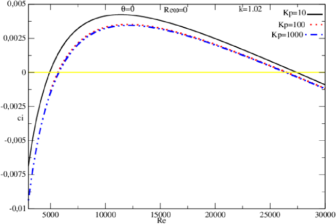
Figure 5: Growth rate $c_{i}$ vs. Reynolds’ number for $k=1.02$, $R_{ew}=0$, $\theta=0\pi$, $Kp=10,100,1000$ and $1$.

This figure 5 shows the behavior of the curve $c_{i}$ vs. Reynolds’ number $R_{e}$ for $k=1.02$, $R_{ew}=0$, $\theta=0$, when $Kp$ increases considerably (strong values of $Kp$). With large values of $Kp$ ($Kp=100,Kp=1000$) the curves have the same behavior and the limit critical Reynolds’ numbers are $R_{ec}\simeq 5770$ and $R_{ec}\simeq 26500$ respectively for the first and second transitions. In the equation (26), we remark that, when $Kp\rightarrow\infty$ the permeability term $\frac{1}{\alpha K_{p}R_{e}}$ vanishes and the model becomes which has been studed in (Hinvi et al.[2]) where the first critical Reynolds’ number is $R_{ec}\simeq 5772.17$.

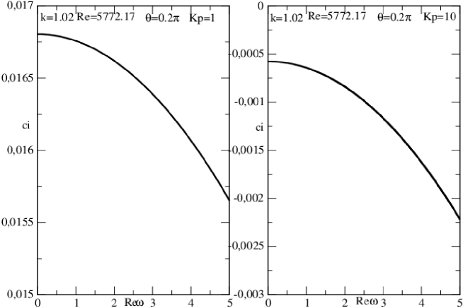
Figure 6: Growth rate $c_{i}$ vs. injection/suction Reynolds’ number $R_{e\omega}$ for $k=1.02$, $R_{e}=5772.17$, $\theta=0.2\pi$. The right frame ($Kp=1$) and the left frame ($Kp=10$).

The figure 6 show growth rate $c_{i}$ vs. injection/suction Reynolds’ number $R_{e\omega}$ for $k=1.02$, $R_{e}=5772.17$, $\theta=0.2\pi$, $Kp=1,10,100$. The both curves are downward, in the left frame we note $c_{i}>0$ i.e the flow is unstable. In the right frame $c_{i}<0$ then the flow is completely stable for this value of $Kp=10$. We conclude that the suction/injection Reynold’s number affects the flow stability and it kept stable for large permeability parameter value.

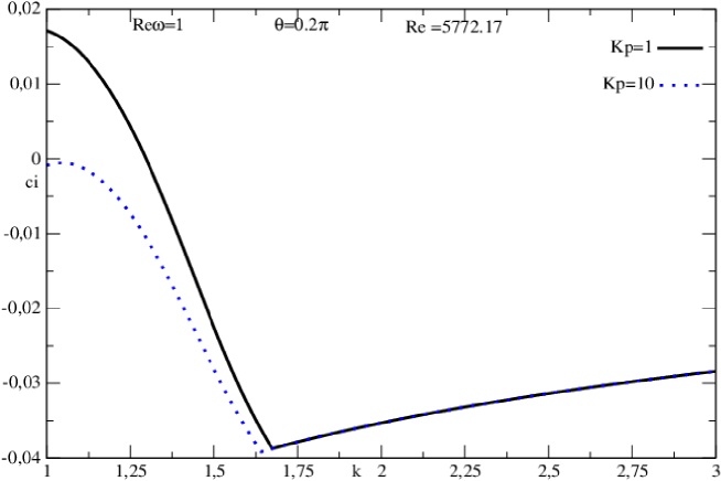
Figure 7: Growth rate $c_{i}$ vs. wave number $k$ for $Re=5772.17$, $\theta=0.2\pi$, $Kp=1$, $Kp=10$ and $R_{e\omega}=1$.

The curves in figure 7 show the appearance of $c_{i}$ as a function of wavenumber $k$, for two different values of $Kp$. We note that for high values of the permeability parameter, the flow is completely stable for any order of $k$. Thus for small $Kp$’s values of the order $1$, the flow remains unstable at the beginning ie for $k<1.5$ and stabilizes after. We also note that after $k=1.73$ the two curves merge. We conclude that there is no special value for $Kp$ to induce any unstability.

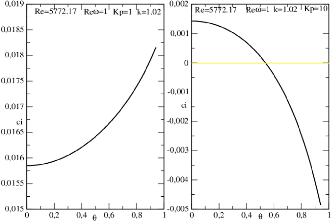
Figure 8: Growth rate $c_{i}$ vs. $\theta(rad)$ for $k=1.02$, $R_{e}=5772.17$, $R_{e\omega}=1$. $Kp=1$ for the left frame and $Kp=10$ for the right frame.

Through figure 8 we have $c_{i}$ vs. $\theta(rad)$. We note that for $Kp=1$, $c_{i}>0$ and the curve is ascendent for all value of $\theta$ and for $kp=10$ the curve is downward but we note unstability in beginning and stability at the end.

6 Conclusion

In this paper, the study of the effect of the Reynolds’ number $R_{e\omega}$ and particular the permeability parameter $Kp$ introduced in Orr-Sommerfeld’s equation by the small suction velocity and permeability of medium, on the stability of the Poiseuille flow in porous medium has been made. The modified Orr-Sommerfeld equation modeling Poiseuille flow in porous medium is deduced. The growth rates $c_{i}$ vs. the parameters of system have been plotted. The previous results analysis allowed us to conclude that all parameters of the system affect the Poiseuille flow stability in porous medium and have a stabilizing effect on the flow.

Acknowlegments

The authors thank IMSP-UAC and Benin gorvernment for financial support.

References

- [1] Chand K., Kumar R. and Sharma S.(). Hydromagnetic Oscillatory Flow through a Porous Medium Bounded by two Vertical Porous Plates with Heat Source and Soret Effect (Advances in Applied Science Research, , ).
- [2] L. A. Hinvi, A. V. Monwanou and J. B. Chabi Orou, (2014). Linear stability analysis of fluid flow between two parallel porous stationary plates., African Review of Physics (2014) 9:0016 p.
- [3] M. Frank White, Book-Viscous Fluid Flow, Second Edition.
- [4] L. A. Hinvi, A. V. Monwanou and J. B. Chabi Orou. Linear stability analysis of hydrodynamic Couette flow in porous medium. Sumetted in (Annals of Faculty Engineering Hunedoara) International Journal Engineering.
- [5] A. V. Monwanou, C. H. Miwadinou and Jean B. Chabi Orou,Stability analysisof boundary layer in Poiseuille flow through a modifed Orr-Sommerfeld equation, Applied Physics Research, Vol, N,ISSN , E-ISSN , pp., DOI:/apr.v4n.
- [6] A. V. Monwanou, (2012) Stability analysis in confined and nonconfined flows, cases of Poiseuille flows and expanding universe.
- [7] E., N. Davidsson . (2007) Stability and Transition in the Suction Boundary Layer and other Shear Flows 2007:04|ISSN:1402-1544|ISRN:LTU-DT–07/04–SE.
- [8] V. A. Monwanou and J. B. Chabi Orou , The Inviscid Instability in an Electrically Conducting Fluid Affected by a Parallel Magnetic Field (The African Review of Physics (2012) 7 : 0044).
- [9] Akkari A. (2012-2013) Mécanique des fluides (notes) I.S.B.S.T.
- [10] H. E. Huntley, Dimensional Analysis, Rinehart, New York, 1951.
- [11] R. Esnault-Pelterie, L ’Analyse dimensionelle, F. Rouge, Lausanne, Switzerland, 1946.
- [12] Robert A. Greenkarm (book) Flow phenomena in porous media ISBN 8-8247-1862-5.
- [13] Kharagpur The Science of Surface and Ground Water; Principles of Ground Water Flow.