Multigrid algorithms for $\boldsymbol{hp}$-version Interior Penalty Discontinuous Galerkin methods on polygonal and polyhedral meshes

Abstract

In this paper we analyze the convergence properties of two-level and W-cycle multigrid solvers for the numerical solution of the linear system of equations arising from $hp$-version symmetric interior penalty discontinuous Galerkin discretizations of second-order elliptic partial differential equations on polygonal/polyhedral meshes. We prove that the two-level method converges uniformly with respect to the granularity of the grid and the polynomial approximation degree $p$, provided that the number of smoothing steps, which depends on $p$, is chosen sufficiently large. An analogous result is obtained for the W-cycle multigrid algorithm, which is proved to be uniformly convergent with respect to the mesh size, the polynomial approximation degree, and the number of levels, provided the number of smoothing steps is chosen sufficiently large. Numerical experiments are presented which underpin the theoretical predictions; moreover, the proposed multilevel solvers are shown to be convergent in practice, even when some of the theoretical assumptions are not fully satisfied.

1 Introduction

The original articles concerned with the construction and mathematical analysis of Discontinuous Galerkin (DG) methods date back over 50 years ago. For hyperbolic partial differential equations, in 1973 Reed & Hill, cf. ReedHill73 , developed the first DG discretization of the neutron transport equation. Independently, DG methods were constructed for elliptic problems based on weakly enforcing Dirichlet boundary conditions; see, for example, Aubin1970 ; Babuska73 ; Lions68 ; nitsche . In particular, we highlight the works of Nitsche nitsche and Baker Baker77 , which form the basis of the class of interior penalty DG methods, cf. also Arn82 ; Whee78 . Since the very early work, DG methods were partially abandoned, in part due to the increase in the number of degrees of freedom compared, for instance, with their conforming counterparts. However, in the last two decades there has been a renewed interest in the field of discontinuous discretizations both from a theoretical and computational viewpoint, cf. CockKarnShu00 ; HestWar ; Rivi08 ; DiPiErn12 , for example. This resurgence is due to the inherent advantages offered by DG schemes, such as, for example, the limited interelement communication, which is restricted only to neighbouring elements, the local conservativity property, the simplicity in treating meshes with hanging nodes, and the development of efficient $hp$-adaptivity refinement strategies. Moreover, recently in BasBotColSub ; Basetal12 ; BasBoetal12 ; Canetal14 it has been shown that the underlying DG polynomial bases may be efficiently constructed in the physical frame, without needing to map local polynomial spaces defined in a given reference/canonical frame. In this way, DG methods can easily deal with general-shaped elements, including polygonal/polyhedral elements, cf. AntBreMar09 ; dg_cfes_2012 ; Canetal14 ; BasBotColSub ; CangianiDongGeorgoulisHouston_2016 ; AntFacRusVer2016 ; CangianiDongGeorgoulis_2016 ; CDGH_book and the recent review paper Anetal16_review . The flexibility of DG methods in handling general meshes has no immediate counterpart in the conforming framework, where the design of suitable finite element spaces for meshes of polygons/polyhedra is far from being a trivial task. Several examples include the Composite Finite Element Method HackSau97 ; HackSau972 , the Polygonal Finite Element Method SukTab04 ; TabSuk08 , the Extended Finite Element Method FriBel10 , the Mimetic Finite Difference Method HymShaStei97 ; BreLipSim05 ; BreLipSha05 ; BreBufSha06 ; BeiManLip_2014 ; Anetal16 and the most recent Virtual Element Method Beietal13 ; BeiBreMarRus16 ; BeiBreMarRus16b ; AntBeiMorVer ; AntBeiScaVer16 .

At present, the design of solvers and preconditioners for DG discretizations on nonstandard grids lends itself to huge developments in the field of numerical analysis. Indeed, to the best of our knowledge, the only study regarding solution techniques for this class of problems is reported in AntGiaHou13 , where a nonoverlapping Schwarz preconditioner for composite DG finite element methods on complicated domains is analyzed, see also the recent paper AntHouSme where optimal bounds for nonoverlapping Schwarz preconditioners for $hp$-version DG methods on standard shape-regular grids have been obtained. In the current article we exploit the theoretical framework developed in Canetal14 to study the performance of a two-level and W-cycle multigrid solver. The possibility to employ general-shaped elements in the physical framework makes the choice of multilevel schemes natural. The flexibility afforded by this approach allows us to define the set of grids needed in the multigrid algorithm by agglomeration; thereby, the definition of the associated subspaces is straightforward, since inter-element continuity is not required. This property overcomes the usual difficulties encountered in the construction of agglomeration multigrid schemes in the conforming framework, where the agglomeration strategy must be followed by a proper definition of the conforming subspaces. In Chanetal98 , for example, the sublevels are obtained by combining a graph based agglomeration algorithm and re-triangulations, thus resulting in a set of non-nested grids, while the associated nested subspaces are defined by introducing suitable interpolation operators. The resulting V-cycle multigrid algorithm converges uniformly with respect to the meshsize $h$ provided that the number of levels is kept fixed.

In this paper we analyze the convergence of a two-level scheme and W-cycle multigrid method for the solution of the linear system of equations arising from the $hp$-version of the interior penalty DG scheme on polygonal/polyhedral meshes Canetal14 , thereby, extending the theoretical framework developed in AntSarVer15 for standard quasi-uniform triangular/quadrilateral meshes, cf. also AntSarVer16 for three-dimensional numerical experiments. Our analysis is based on the smoothing and approximation properties associated with the proposed method: the former corresponds to a Richardson iteration, whose study requires a result concerning the spectral properties of the stiffness matrix, while the latter is inherent to the interior penalty DG scheme itself and exploits the error estimates derived in Canetal14 . We show that, under suitable assumptions on the agglomerated coarse grid, both the two-level and the W-cycle multigrid schemes converge uniformly with respect to the granularity of the underlying partition and the polynomial approximation degree $p$, provided that the number of smoothing steps is chosen of order $p^{2+\mu}$, with $\mu=0,1$. Throughout the analysis, we also track the dependence of the error reduction factor of the two solvers on the geometric properties of the agglomerated grids, thereby recovering a similar result to the case when standard quasi-uniform triangular and/or quadrilateral meshes are employed.

The rest of this paper is organized as follows. In Section 2 we introduce the interior penalty DG scheme for the discretization of second-order elliptic problems on general meshes consisting of polygonal/polyhedral elements. Then in Section 3, we recall some preliminary analytical results concerning this class of schemes. In Section 4 we define the multilevel framework and introduce several technical results. We then focus first on the analysis of the two-level method, followed by the extension to the W-cycle multigrid solver. The main theoretical results are investigated through a series of numerical experiments presented in Section 6, where we also present a comparison with an unsmoothed Algebraic Multigrid method. Finally, in Section 7 we draw some conclusions.

2 Model problem and discretization

We consider the weak formulation of the Poisson problem, subject to a homogeneous Dirichlet boundary condition: find $u\in V=H^{2}(\Omega)\cap H_{0}^{1}(\Omega)$ such that

$$\int_{\Omega}\nabla u\cdot\nabla v\ dx=\int_{\Omega}fv\ dx\,\qquad\forall v\in V,$$ (1)

with $\Omega\in\mathbb{R}^{d}$, $d=2,3$, a convex polygonal/polyhedral domain with Lipschitz boundary and $f$ a given function in $L^{2}(\Omega)$.

For the sake of brevity, throughout this article, we write $x\lesssim y$ and $x\gtrsim y$ in lieu of $x\leq Cy$ and $x\geq Cy$, respectively, for a positive constant $C$ independent of the discretization parameters. Moreover, $x\approx y$ means that there exist constants $C_{1},C_{2}>0$ such that $C_{1}y\leq x\leq C_{2}y$. When required, the constants will be written explicitly.

In view of the forthcoming multigrid analysis, we denote by $\{\mathcal{T}_{j}\}_{j=1}^{J}$ a sequence of partitions of the domain $\Omega$, each of which consists of disjoint open polygonal/polyhedral elements $\kappa$ of diameter $h_{\kappa}$, such that $\overline{}\Omega=\bigcup_{\kappa\in\mathcal{T}_{j}}\bar{}\kappa$, $j=1,\dots,J$. We denote the mesh size of $\mathcal{T}_{j}$, $j=1,\dots,J$, by $h_{j}=\max_{\kappa\in\mathcal{T}_{j}}h_{\kappa}$. To each $\mathcal{T}_{j}$, $j=1,\dots,J$, we associate the corresponding DG finite element space $V_{j}$, $j=1,\dots,J$, defined as

$$V_{j}=\{v\in L^{2}(\Omega):v|_{\kappa}\in\mathcal{P}_{p_{j}}(\kappa),\kappa\in\mathcal{T}_{j}\},$$ (2)

where $\mathcal{P}_{p_{j}}(\kappa)$ denotes the space of polynomials of total degree at most $p_{j}\geq 1$ on $\kappa\in\mathcal{T}_{j}$. A suitable choice of the sequences $\{\mathcal{T}_{j}\}_{j=1}^{J}$ and $\{V_{j}\}_{j=1}^{J}$ leads to the so-called $h$- and $p$-multigrid schemes. In particular, the $h-$multigrid method is based on employing a constant polynomial approximation degree for each $j$, $j=1,\dots,J$, (i.e., $p_{j}=p$), on a set of nested partitions $\{\mathcal{T}_{j}\}_{j=1}^{J}$, such that the coarse level $\mathcal{T}_{j-1}$, $j=2,\dots,J$, is obtained by agglomeration from $\mathcal{T}_{j}$ in such a way that

$$h_{j-1} \lesssim h_{j} \leq h_{j-1}\qquad\forall j=2,\dots,J,$$ (3)

i.e., we assume a bounded variation hypothesis between subsequent levels. In the $p$-multigrid method, the partition is kept fixed for any $j$, $j=1,\dots,J$, while we assume that the polynomial degrees vary moderately from one level to another, i.e.,

$$p_{j-1}\leq p_{j}\lesssim p_{j-1}\qquad\forall j=2,\dots,J.$$ (4)

Note that with the above choices we obtain nested finite element spaces $V_{j}$, $j=1,\dots,J$, i.e., $V_{1}\subseteq V_{2}\subseteq\dots\subseteq V_{J}$.

2.1 Grid assumptions

In this section, we outline some key definitions and assumptions. For any $\mathcal{T}_{j}$, $j=1,\dots,J$, when no hanging nodes/edges are included in the partition, we define the interfaces of the mesh $\mathcal{T}_{j}$ as the set of $(d-1)$-dimensional facets of the elements $\kappa\in\mathcal{T}_{j}$. The presence of hanging nodes/edges, on the other hand, can be handled by defining the interfaces of $\mathcal{T}_{j}$ as the intersection of the $(d-1)$-dimensional facets of neighboring elements. This implies that, for $d=2$, an interface will always consist of a piecewise linear line segment, i.e., they consist of a set of $(d-1)$–dimensional simplices. However, in general for $d=3$, the interfaces of $\mathcal{T}_{j}$ will consist of general polygonal surfaces. Thereby, we assume that each planar section of each interface of an element $\kappa\in\mathcal{T}_{j}$ may be subdivided into a set of co-planar triangles ($(d-1)$–dimensional simplices). We refer to these $(d-1)$–dimensional simplices, whose union form the interfaces of $\mathcal{T}_{j}$, as faces. With this notation, we assume that the sub-tessalation of element interfaces into $(d-1)$–dimensional simplices is given. We denote by $\mathcal{F}_{j}$ the set of all mesh faces; moreover, we have that $\mathcal{F}_{j}=\mathcal{F}_{j}^{I}\cup\mathcal{F}_{j}^{B}$, where $\mathcal{F}_{j}^{I}$ is the set of interior element faces of $\mathcal{T}_{j}$, such that $F\subseteq\partial\kappa^{+}\cap\partial\kappa^{-}$ for any $F\in\mathcal{F}_{j}^{I}$, where $\kappa^{\pm}$ are two adjacent elements in $\mathcal{T}_{j}$. The set $\mathcal{F}_{j}^{B}$ contains the boundary element faces, i.e., $F\subset\partial\Omega$ for $F\in\mathcal{F}_{j}^{B}$.

We are now ready to introduce the following assumptions on the partitions $\mathcal{T}_{j}$, $j=1,\dots,J$; cf. CangianiDongGeorgoulis_2016 . In the case of the $h$-multigrid scheme, these assumptions must be satisfied for the meshes generated by the underlying agglomeration process.

Assumption 2.1

Given $\kappa\in\mathcal{T}_{j}$, there exists a set of nonoverlapping (not necessarily shape-regular) $d$–dimensional simplices $T_{\ell}\subseteq\kappa$, $\ell=1,2,\ldots,n_{\kappa}$, such that, for any face $F\subset\partial\kappa$, $\overline{F}=\partial\overline{\kappa}\cap\partial\overline{T_{\ell}}$, for some $\ell$,

$$\cup_{\ell=1}^{n_{\kappa}}\overline{T}_{\ell}\subseteq\overline{\kappa},$$ (5)

and the diameter $h_{\kappa}$ of $\kappa$ can be bounded by

$$h_{\kappa}\lesssim\frac{d|T_{\ell}|}{|F|}, \ell=1,2,\ldots,n_{\kappa}.$$

Remark 1

We point out that Assumption 2.1 does not put a restriction on either the number of faces that an element possesses, or indeed the measure of a face of an element $\kappa\in\mathcal{T}_{j}$, relative to the measure of the element itself. This will be particularly important in the agglomeration procedure employed within our $h$-multigrid method, since as the number of levels increases, the number of faces that the resulting agglomerated elements may contain grows, while their measure, relative to the element measure, may degenerate.

Remark 2

As pointed out in CangianiDongGeorgoulis_2016 , meshes obtained by agglomeration of a finite number of polygons that are uniformly star-shaped with respect to the largest inscribed ball will automatically satisfy Assumption 2.1. Therefore, from the practical point of view, given a fine-level mesh $\mathcal{T}_{J}$ consisting of uniformly star-shaped elements, a finite number of agglomeration steps will produce a sequence of admissible grids. To allow the number of agglomeration levels to increase arbitrarily one can either i) ensure that each of the agglomerated meshes satisfy Assumption 2.1; ii) check, at each level, that the (slightly more restrictive) shape-regularity criterion on the agglomerates is satisfied.

Assumption 2.2

For any $\kappa\in\mathcal{T}_{j}$, $j=1,\dots,J$, we assume that $h_{\kappa}^{d}\geq|\kappa|\gtrsim h_{\kappa}^{d},$ with $d=2,3$.

We next introduce the following additional mesh condition, cf. CangianiDongGeorgoulisHouston_2016 , which will be required in order to obtain the inverse estimates presented in Lemma 4.

Assumption 2.3

Every polytopic element $\kappa\in\mathcal{T}_{j}$, admits a sub-triangulation into at most $m_{\kappa}$ shape-regular simplices $\mathfrak{s}_{i}$, $i=1,2,\dots,m_{\kappa}$, such that $\bar{\kappa}=\cup_{i=1}^{m_{\kappa}}\bar{\mathfrak{s}}_{i}$ and

$$|\mathfrak{s}_{i}|\gtrsim|\kappa|$$

for all $i=1,\dots,m_{\kappa}$, for some $m_{\kappa}\in\mathbb{N}$. The hidden constant is independent of $\kappa$ and $\mathcal{T}_{j}$.

In view of the approximation result that will be presented in the next section we also introduce the following additional assumption.

Assumption 2.4

Let $\mathcal{T}_{j}^{\sharp}=\{\mathcal{K}\}$, denote a covering of $\Omega$ consisting of shape-regular $d$-dimensional simplices $\mathcal{K}$. We assume that, for any $\kappa\in\mathcal{T}_{j}$, there exists $\mathcal{K}\in\mathcal{T}_{j}^{\sharp}$ such that $\kappa\subset\mathcal{K}$ and

$${\color[rgb]{0,0,0}\max_{\kappa\in{\cal T}_{j}}\,}\textnormal{card}\left\{\kappa^{\prime}\in{\cal T}_{j}:\kappa^{\prime}\cap\mathcal{K}\neq\emptyset,~{}\mathcal{K}\in\mathcal{T}_{j}^{\sharp}~{}\mbox{ such that }~{}\kappa\subset\mathcal{K}\right\}\lesssim 1.$$

Consequently, for each pair $\kappa$, $\mathcal{K}\in\mathcal{T}_{j}^{\sharp}$, with $\kappa\subset\mathcal{K}$, $\textnormal{diam}(\mathcal{K})\lesssim h_{\kappa}.$

We also need the following assumption on the quality of agglomerated grids.

Assumption 2.5

For any $F\in\mathcal{F}_{j}\cap\mathcal{F}_{j-1}$, $j=2,\ldots,J$, we denote by $\kappa^{\pm}_{j}$ and $\kappa^{\pm}_{j-1}$ the neighboring elements sharing the face $F$ in $\mathcal{T}_{j}$ and $\mathcal{T}_{j-1}$, respectively. We assume that there exists $\Theta>0$ such that

$$1<\frac{h_{\kappa_{j-1}^{\pm}}}{h_{\kappa_{j}^{\pm}}}\leq\Theta\quad\forall F\in\mathcal{F}_{j}\cap\mathcal{F}_{j-1}.$$

We remark that Assumption 2.5 is satisfied if the agglomeration algorithm preserves the shape-regularity of the elements. In Figure 1, we show two examples of possible macroelements: the agglomerate on the left is not suitable to guarantee Assumption 2.5 due to the presence of a dominant dimension, while the element on the right can be considered appropriate. Moreover, we note that the fulfilment of Assumption 2.5 can be considered a good criterion in evaluating the quality of the agglomerated grids employed in the multigrid algorithm, cf. Figure 1 for an illustration.

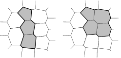
Figure 1: Examples of agglomerated elements. The agglomerated element on the left violates Assumption 2.5 whereas the one on the right satisfies Assumption 2.5.

Finally, to keep the notation as simple as possible, in the forthcoming analysis we will assume that, for any $j=1,\dots,J$, the decompositions $\mathcal{T}_{j}$ are quasi-uniform, i.e., $h_{j}\approx\min_{\kappa\in\mathcal{T}_{j}}h_{\kappa}$. We remark that the above assumption can be weakened and only a local bounded variation property is needed for our theoretical analysis; see Remark 4 below for details.

2.2 DG formulation

The definition of the proceeding DG method is based on employing suitable jump and average operators. To this end, for (sufficiently smooth) vector- and scalar-valued functions $\boldsymbol{\tau}$ and $v$, respectively, we define jumps and averages across $F\in\mathcal{F}_{j}$, $j=1,\ldots,J$, as follows:

$$\llbracket\boldsymbol{\tau}\rrbracket =\boldsymbol{\tau}^{+}\cdot\mathbf{n}^{+}+\boldsymbol{\tau}^{-}\cdot\mathbf{n}^{-},\quad \{\mathchoice{{}\mkern-6.0mu}{{}\mkern-6.0mu}{{}\mkern-6.0mu}{}\{\boldsymbol{\tau}\}\mathchoice{{}\mkern-6.0mu}{{}\mkern-6.0mu}{{}\mkern-6.0mu}{}\} =\frac{\boldsymbol{\tau}^{+}+\boldsymbol{\tau}^{-}}{2},\qquad F\in\mathcal{F}_{j}^{I},$$

$$\llbracket v\rrbracket =v^{+}\mathbf{n}^{+}+v^{-}\mathbf{n}^{-}, \{\mathchoice{{}\mkern-6.0mu}{{}\mkern-6.0mu}{{}\mkern-6.0mu}{}\{v\}\mathchoice{{}\mkern-6.0mu}{{}\mkern-6.0mu}{{}\mkern-6.0mu}{}\} =\frac{v^{+}+v^{-}}{2},\qquad F\in\mathcal{F}_{j}^{I},$$

$$\llbracket v\rrbracket =v^{+}\mathbf{n}^{+}, \{\mathchoice{{}\mkern-6.0mu}{{}\mkern-6.0mu}{{}\mkern-6.0mu}{}\{\boldsymbol{\tau}\}\mathchoice{{}\mkern-6.0mu}{{}\mkern-6.0mu}{{}\mkern-6.0mu}{}\} =\boldsymbol{\tau}^{+}, F\in\mathcal{F}_{j}^{B},$$

where $v^{\pm}$ and $\boldsymbol{\tau}^{\pm}$ denote the traces of $v$ and $\boldsymbol{\tau}$ on $F$ taken from the interior of $\kappa^{\pm}$, respectively, and $\mathbf{n}^{\pm}$ the outward unit normal vectors to $\partial\kappa^{\pm}$, respectively, cf. Arnetal01 . On any level $j$, $j=1,\dots,J$, we consider the bilinear form $\mathcal{A}_{j}(\cdot,\cdot):V_{j}\times V_{j}\rightarrow\mathbb{R}$, corresponding to the symmetric interior penalty DG method, defined by

$$\mathcal{A}_{j}(u,v)= \sum_{\kappa\in\mathcal{T}_{j}}\int_{\kappa}\nabla u\cdot\nabla v\ dx-\sum_{F\in\mathcal{F}_{j}}\int_{F}\left(\{\mathchoice{{}\mkern-6.0mu}{{}\mkern-6.0mu}{{}\mkern-6.0mu}{}\{\nabla u\}\mathchoice{{}\mkern-6.0mu}{{}\mkern-6.0mu}{{}\mkern-6.0mu}{}\}\cdot\llbracket v\rrbracket+\llbracket u\rrbracket\cdot\{\mathchoice{{}\mkern-6.0mu}{{}\mkern-6.0mu}{{}\mkern-6.0mu}{}\{\nabla v\}\mathchoice{{}\mkern-6.0mu}{{}\mkern-6.0mu}{{}\mkern-6.0mu}{}\}\right)\ ds$$

$$+\sum_{F\in\mathcal{F}_{j}}\int_{F}\sigma_{j}\llbracket u\rrbracket\cdot\llbracket v\rrbracket\ ds,$$ (6)

where $\sigma_{j}\in L^{\infty}(\mathcal{F}_{j})$ denotes the interior penalty stabilization function $\sigma_{j}:\mathcal{F}_{j}\rightarrow\mathbb{R}^{+}$, which is defined by

$$\sigma_{j}(x)=\left\{\begin{aligned} &C_{\sigma}^{j}\max_{\kappa\in\{\kappa^{+},\kappa^{-}\}}\Big{\{}\frac{p_{j}^{2}}{h_{\kappa}}\Big{\}},\ &x\in F,~{}F\in\mathcal{F}_{j}^{I},\ F\subset\partial\kappa^{+}\cap\partial\kappa^{-},\\ &C_{\sigma}^{j}\frac{p_{j}^{2}}{h_{\kappa}},\ &x\in F,~{}F\in\mathcal{F}_{j}^{B},\ F\subset\partial\kappa^{+}\cap\partial\Omega,\\ \end{aligned}\right.$$ (7)

with $C_{\sigma}^{j}>0$ independent of $p_{j}$, $|F|$ and $|\kappa|$.

In this article, we develop two-level and W-cycle multigrid schemes to compute the solution of the following problem on the finest level $J$: find $u_{J}\in V_{J}$ such that

$$\mathcal{A}_{J}(u_{J},v_{J})=\int_{\Omega}fv_{J}\ dx\quad\forall v_{J}\in V_{J}.$$ (8)

3 Preliminary results

We first recall the following trace-inverse inequality for polygonal/polyhedral elements.

Lemma 1

Assume that the sequence of meshes $\mathcal{T}_{j}$, $j=1,\dots,J$, satisfies Assumption 2.1. Let $\kappa\in\mathcal{T}_{j}$, $j=1,\dots,J$, be a polygonal/polyhedral element, then the following bound holds

$$\|v\|_{L^{2}(\partial\kappa)}^{2}\leq{\color[rgb]{0,0,0}\mathsf{C}^{j}_{\mathsf{inv}}}\frac{p_{j}^{2}}{h_{\kappa}}\|v\|_{L^{2}(\kappa)}^{2} \forall\,v\in\mathcal{P}_{p_{j}}(\kappa),$$ (9)

where ${\color[rgb]{0,0,0}\mathsf{C}^{j}_{\mathsf{inv}}}$ is independent of $|\kappa|$, $p_{j}$ and $v$.

The proof can be obtained with trivial modifications with respect to the ones given in CangianiDongGeorgoulis_2016 ; CDGH_book . For the sake of completeness we report it and refer to CangianiDongGeorgoulis_2016 ; CDGH_book for further details.

Proof

From Assumption 2.1, there exists a set of nonoverlapping (not necessarily shape-regular) $d$-simplicial elements $T_{\ell}\subseteq\kappa$ such that, given a face $F\subset\partial\kappa$, for some $\ell$, $1\leq\ell\leq n_{\kappa}$, $\overline{F}=\partial\overline{\kappa}\cap\partial\overline{T_{\ell}}$. Therefore,

$$\|u\|_{L^{2}(\partial\kappa)}^{2}=\sum_{F\subset\partial\kappa}\|u\|_{L^{2}(F)}^{2}\lesssim p_{j}^{2}\sum_{\ell=1}^{n_{\kappa}}\frac{|F|}{|T_{\ell}|}\|u\|_{L^{2}(T_{\ell})}^{2}\lesssim\frac{p_{j}^{2}}{h_{\kappa}}\sum_{\ell=1}^{n_{\kappa}}\|u\|_{L^{2}(T_{\ell})}^{2}\leq\frac{p_{j}^{2}}{h_{\kappa}}\|u\|_{L^{2}(\kappa)}^{2},$$

as required. Here, in the first inequality we have employed the following classical trace-inverse estimate on $d$-simplicial elements

$$\|u\|_{L^{2}(F)}^{2}\lesssim p_{j}^{2}\frac{|F|}{|T_{\ell}|}\|u\|_{L^{2}(T_{\ell})}^{2},$$

cf. Sch98 ; Geo08 , for example; the second bound exploits Assumption 2.1, namely, that $|F|{|T_{\ell}|}^{-1}\lesssim dh^{-1}_{\kappa}$.

Next, we endow the finite element spaces $V_{j}$, $j=1,\dots,J$, with the following DG norm:

$$\|w\|_{DG,j}^{2}=\sum_{\kappa\in\mathcal{T}_{j}}\int_{\kappa}|\nabla w|^{2}\ dx+\sum_{F\in\mathcal{F}_{j}}\int_{F}\sigma_{j}|\llbracket w\rrbracket|^{2}\ ds.$$ (10)

The well–posedness of the DG formulation is established in the following lemma

Lemma 2

Assume that the sequence of meshes $\mathcal{T}_{j}$, $j=1,\dots,J$, satisfies Assumption 2.1 and that the constant $C_{\sigma}^{j}$, $j=1,\dots,J$, appearing in the definition (7) of the stabilization function is chosen sufficiently large. Then, the following continuity and coercivity bounds, respectively, hold

$$\mathcal{A}_{j}(u,v) \leq{\color[rgb]{0,0,0}\mathsf{C}_{\mathsf{cont}}}\|u\|_{DG,j}\|v\|_{DG,j}\quad \forall u,v\in V_{j},$$ (11)

$$\mathcal{A}_{j}(u,u) \geq{\color[rgb]{0,0,0}\mathsf{C}_{\mathsf{coer}}}\|u\|_{DG,j}^{2}\quad \forall u\in V_{j},$$ (12)

where ${\color[rgb]{0,0,0}\mathsf{C}_{\mathsf{cont}}}$ and ${\color[rgb]{0,0,0}\mathsf{C}_{\mathsf{coer}}}$ are positive constants, independent of the discretization parameters.

The proceeding error estimates are based on the following approximation result, which is a simplified version of the analogous bound presented in (Canetal14, , Proof of Theorem 5.2). To this end, we define $\mathcal{E}:H^{s}(\Omega)\rightarrow H^{s}({\mathbb{R}}^{d})$, $s\in{\mathbb{N}}_{0}$, such that $\mathcal{E}v|_{\Omega}=v$, to denote the extension operator presented in Stein stein .

Lemma 3

Assume that Assumptions 2.1 and 2.4 hold. Let $v|_{\kappa}\in H^{k}(\kappa)$, $k>d/2$, such that $\mathcal{E}v|_{\mathcal{K}}\in H^{k}(\mathcal{K})$, for each $\kappa\in\mathcal{T}_{j}$, $j=1,\dots,J$, where $\kappa\subset\mathcal{K}$, $\mathcal{K}\in\mathcal{T}_{j}^{\sharp}$. Then there exists a projection operator $\widetilde{\Pi}_{j}:L^{2}(\Omega)\rightarrow V_{j}$ such that

$$\|v-\tilde{\Pi}_{j}v\|_{DG,j} \leq{\color[rgb]{0,0,0}\mathsf{C}^{j}_{\mathsf{interp}}}\frac{h_{j}^{s-1}}{p_{j}^{k{\color[rgb]{0,0,0}-1-\mu/2}}}\|v\|_{H^{k}(\Omega)},$$ (13)

where $s=\min\{p_{j}+1,k\}$, and the constant ${\color[rgb]{0,0,0}\mathsf{C}^{j}_{\mathsf{interp}}}$ depends on the shape-regularity constant of the covering $\mathcal{T}_{j}^{\sharp}$, but is independent of the discretization parameters, as well as the number of faces per element and the relative measure of the faces. Here, $\mu=0$ whenever a $p-$optimal interpolant can be constructed and $\mu=1$ otherwise.

Next, we state error bounds for the underlying interior penalty DG scheme in terms of both the DG and $L^{2}(\Omega)$-norms.

Theorem 3.1

Assume that Assumptions 2.1 and 2.4 hold. Denote by $u_{j}\in V_{j}$, $j=1,\ldots,J$, the DG solution of problem (8) posed on level $j$, i.e.,

$$\mathcal{A}_{j}(u_{j},v_{j})=\int_{\Omega}fv_{j}\ dx\quad\forall v_{j}\in V_{j}.$$

If the solution $u$ of (1) satisfies $u|_{\kappa}\in H^{k}(\kappa)$, $k>1+d/2$, such that $\mathcal{E}u|_{\mathcal{K}}\in H^{k}(\mathcal{K})$, for each $\kappa\in\mathcal{T}_{j}$, $j=1,\dots,J$, where $\kappa\subset\mathcal{K}$, $\mathcal{K}\in\mathcal{T}_{j}^{\sharp}$, then the following bounds hold

$$\|u-u_{j}\|_{DG,j} \leq{\color[rgb]{0,0,0}\mathsf{G}^{j}}\frac{h_{j}^{s-1}}{p_{j}^{k{\color[rgb]{0,0,0}-1-\mu/2}}}\|u\|_{H^{k}(\Omega)},$$ (14)

$$\|u-u_{j}\|_{L^{2}(\Omega)} \leq{\color[rgb]{0,0,0}\mathsf{C}^{j}_{L^{2}}}\frac{h_{j}^{s}}{p_{j}^{k{\color[rgb]{0,0,0}-\mu}}}\|u\|_{H^{k}(\Omega)},$$ (15)

where $s=\min\{p_{j}+1,k\}$ and the constants ${\color[rgb]{0,0,0}\mathsf{G}^{j}}$ and ${\color[rgb]{0,0,0}\mathsf{C}^{j}_{L^{2}}}$ are independent of the discretization parameters. Here, $\mu=0$ whenever a $p-$optimal interpolant can be constructed and $\mu=1$ otherwise.

Before proceeding with the proof, we point out that the above error bounds hold provided Assumptions 2.1 and 2.4 are satisfied; however, we stress that no limitation is placed on the maximum number of faces that each polygonal/polyhedral element may possess. Moreover, there is no restriction on the relative size of each face of an element compared to its diameter.

Proof

The error bound (14) stems from the general result derived in (Canetal14, , Theorem 5.2) under the condition that Assumptions 2.1 and 2.4 hold. Thereby, we now proceed with the proof of the bound on the $L^{2}(\Omega)$-norm of the error, cf. (15). To this end, we employ a standard duality argument: let $w\in V$, be the solution of the problem

$${\color[rgb]{0,0,0}\mathcal{A}_{j}(v,w)}=\int_{\Omega}(u-u_{j})v\ dx\qquad\forall v\in V,$$

$j=1,\ldots,J$. Exploiting a standard elliptic regularity assumption, we note that

$$\|w\|_{H^{2}(\Omega)}\lesssim\|u-u_{j}\|_{L^{2}(\Omega)}.$$

According to Galerkin orthogonality, we immediately obtain

$$\|u-u_{j}\|_{L^{2}(\Omega)}^{2} =\mathcal{A}_{j}(u-u_{j},w)$$

$$=\mathcal{A}_{j}(u-u_{j},w-w_{I})$$

$$\lesssim\|u-u_{j}\|_{DG,j}\|w-w_{I}\|_{DG,j}$$

for all $w_{I}\in V_{j}$. Hence, selecting $w_{I}=\tilde{\Pi}_{j}w$, employing (13) gives

$$\|w-w_{I}\|_{DG,j}\lesssim{\color[rgb]{0,0,0}\mathsf{C}^{j}_{\mathsf{interp}}}\frac{h_{j}}{p_{j}^{1/2}}\|w\|_{H^{2}(\Omega)}\lesssim{\color[rgb]{0,0,0}\mathsf{C}^{j}_{\mathsf{interp}}}\frac{h_{j}}{p_{j}^{{\color[rgb]{0,0,0}1-\mu/2}}}\|u-u_{j}\|_{L^{2}(\Omega)},$$ (16)

which together with (14) gives the desired result.

Equipped with Assumption 2.3, we now quote the following result from CangianiDongGeorgoulisHouston_2016 ; for brevity the proof is omitted. However, we point out that the proof presented in CangianiDongGeorgoulisHouston_2016 holds under slightly weaker mesh conditions; for simplicity of presentation, this level of detail is omitted.

Lemma 4

Assume that Assumptions 2.2 and 2.3 hold. Then, for any $v\in V_{j}$, $j=1,\ldots,J$, the following inverse estimate holds

$$\|\nabla u\|_{L^{2}(\kappa)}^{2}\leq{\color[rgb]{0,0,0}\mathsf{C}_{\mathsf{I}}^{j}}p_{j}^{4}h_{\kappa}^{-2}\|u\|_{L^{2}(\kappa)}^{2},$$ (17)

where ${\color[rgb]{0,0,0}\mathsf{C}_{\mathsf{I}}^{j}}>0$ is independent of the discretization parameters.

The inverse estimate presented in Lemma 4 is fundamental to the proof of the following upper bound on the maximum eigenvalue of $\mathcal{A}_{j}(\cdot,\cdot)$. We recall that the analogous result on standard grids can be found in AntHou , cf. also AntHou13 .

Theorem 3.2

Given that Assumptions 2.1, 2.2, and 2.3 hold, then for any $u\in V_{j}$, $j=1,\ldots,J$, we have that

$$\mathcal{A}_{j}(u,u)\leq{\color[rgb]{0,0,0}\mathsf{C}^{j}_{\mathsf{eig}}}\frac{p_{j}^{4}}{h_{j}^{2}}\|u\|_{L^{2}(\Omega)}^{2},$$ (18)

where the constant ${\color[rgb]{0,0,0}\mathsf{C}^{j}_{\mathsf{eig}}}$ is independent of the discretization parameters.

Proof

Given the continuity of the bilinear forms $\mathcal{A}_{j}(\cdot,\cdot)$ stated in Lemma 2, we restrict ourselves to estimate the two terms involved in the DG norm. The local contributions of the $H^{1}$ seminorm can be simply bounded by applying Lemma 4 and the quasi-uniformity of the partition, i.e.,

$$\sum_{\kappa\in\mathcal{T}_{j}}|u|_{H^{1}(\kappa)}^{2}\leq\sum_{\kappa\in\mathcal{T}_{j}}{\color[rgb]{0,0,0}\mathsf{C}_{\mathsf{I}}^{j}}p_{j}^{4}h_{\kappa}^{-2}\|u\|_{L^{2}(\kappa)}^{2}\leq{\color[rgb]{0,0,0}\left(\max_{\kappa\in\mathcal{T}_{j}}{\color[rgb]{0,0,0}\mathsf{C}_{\mathsf{I}}^{j}}\right)}\frac{p_{j}^{4}}{h_{j}^{2}}\|u\|_{L^{2}(\Omega)}^{2}.$$ (19)

To bound the norm of the jump across $F\in\mathcal{F}_{j}$, we employ the inverse inequality (9); thereby, we get

$$\sum_{F\in\mathcal{F}_{j}}\|\sigma_{j}^{1/2}\llbracket u\rrbracket\|_{L^{2}(F)}^{2}\lesssim ~{}\sum_{\kappa\in\mathcal{T}_{j}}\|\sigma_{j}^{1/2}\llbracket u\rrbracket\|_{L^{2}(\partial\kappa)}^{2}\lesssim~{}C^{j}_{\sigma}{\color[rgb]{0,0,0}\mathsf{C}^{j}_{\mathsf{inv}}}\frac{p_{j}^{4}}{h_{j}^{2}}\|u\|_{L^{2}(\Omega)}^{2}.$$ (20)

The statement of the theorem immediately follows based on summing the above bounds.

The theoretical results derived in this section form the basis of the analysis of the proposed multigrid algorithms presented in the following section.

4 Two-level and W-cycle multigrid algorithms

The forthcoming analysis is based on the classical multigrid theoretical framework already employed in AntSarVer15 for high-order DG schemes on standard quasi-uniform meshes. The two key ingredients in the construction of our proposed multigrid schemes are the inter-grid transfer operators and the smoothing scheme. The prolongation operator connecting the space $V_{j-1}$ to $V_{j}$, $j=2,\ldots,J$, is denoted by $I^{j}_{j-1}:V_{j-1}\rightarrow V_{j}$, while its adjoint with respect to the $L^{2}(\Omega)$-inner product $(\cdot,\cdot)$ is the restriction operator $I^{j-1}_{j}:V_{j}\rightarrow V_{j-1}$ defined by

$$(I^{j}_{j-1}v,w)=(v,I^{j-1}_{j}w)\qquad\forall v\in V_{j-1},w\in V_{j}.$$

As a smoothing scheme, we choose a Richardson iteration, whose operator is defined as:

$$B_{j}=\Lambda_{j}\textnormal{Id}_{j},$$ (21)

with $\textnormal{Id}_{j}$ the identity operator on level $V_{j}$, and $\Lambda_{j}\in\mathbb{R}$ is an upper bound for the spectral radius of the operator $A_{j}:V_{j}\rightarrow V_{j}$, defined by

$$(A_{j}u,v)=\mathcal{A}_{j}(u,v)\quad\forall u,v\in V_{j},~{}~{}j=1,\ldots,J.$$ (22)

For the definition of the solvers, we first address the two-level method. Given the problem $A_{J}u_{J}=f_{J}$ with $A_{J}:V_{J}\rightarrow V_{J}$ defined according to (22), and $f_{J}\in V_{J}$ such that

$$(f_{J},v)=\int_{\Omega}fv\ dx\quad\forall v\in V_{J},$$

in Algorithm 1 we outline the two-level cycle, where $\mathsf{MG_{2lvl}}(z_{0},m_{1},m_{2})$ denotes the approximate solution obtained after one iteration, with initial guess $z_{0}$ and $m_{1}$, $m_{2}$ pre- and post-smoothing steps, respectively.

Algorithm 1 Two-level scheme

Pre-smoothing:

for $i=1,\dots,m_{1}$ do

     $z^{(i)}=z^{(i-1)}+B_{J}^{-1}(f_{J}-A_{J}z^{(i-1)});$

end for

Coarse grid correction:

$r_{J-1}=I_{J}^{J-1}(f_{J}-A_{J}z^{(m_{1})})$;

$e_{J-1}=A_{J-1}^{-1}r_{J-1}$;

$z^{(m_{1}+1)}=z^{(m_{1})}+I_{J-1}^{J}e_{J-1}$;

Post-smoothing:

for $i=m_{1}+2,\dots,m_{1}+m_{2}+1$ do

     $z^{(i)}=z^{(i-1)}+B_{J}^{-1}(f_{J}-A_{J}z^{(i-1)});$

end for

$\mathsf{MG_{2lvl}}(z_{0},m_{1},m_{2})=z^{(m_{1}+m_{2}+1)}.$

As a multilevel extension of Algorithm 1, we consider a standard W-cycle scheme. On level $j$, we consider $A_{j}z=g$, for a given $g\in V_{j}$. The approximate solution obtained by applying the $j$-th level iteration to the above linear system, with initial guess $z_{0}$ and $m_{1}$, $m_{2}$ pre- and post-smoothing steps, respectively, is denoted by $\mathsf{MG}_{\mathcal{W}}(j,g,z_{0},m_{1},m_{2})$. On the coarsest level $j=1$, the corresponding subproblem is solved based on employing a direct method, i.e.,

$$\mathsf{MG}_{\mathcal{W}}(1,g,z_{0},m_{1},m_{2})=A_{1}^{-1}g,$$

while for $j>1$ we apply the recursive procedure outlined in Algorithm 2. We observe that Algorithm 1 can be considered as a special case of Algorithm 2, corresponding to $J=2$.

Algorithm 2 Multigrid W-cycle scheme

if $j=1$ then

     $\mathsf{MG}_{\mathcal{W}}(1,g,z_{0},m_{1},m_{2})=A_{1}^{-1}g.$

else

     Pre-smoothing:

     for $i=1,\dots,m_{1}$ do

         $z^{(i)}=z^{(i-1)}+B_{j}^{-1}(g-A_{j}z^{(i-1)});$

     end for

     Coarse grid correction:

     ${\color[rgb]{0,0,0}r_{j-1}}=I_{j}^{j-1}(g-A_{j}z^{(m_{1})})$;

     $\overline{e}_{j-1}=\mathsf{MG}_{\mathcal{W}}(j-1,r_{j-1},0,m_{1},m_{2})$;

     $e_{j-1}=\mathsf{MG}_{\mathcal{W}}(j-1,r_{j-1},\overline{e}_{j-1},m_{1},m_{2})$;

     $z^{(m_{1}+1)}=z^{(m_{1})}+I_{j-1}^{j}e_{j-1}$;

     Post-smoothing:

     for $i=m_{1}+2,\dots,m_{1}+m_{2}+1$ do

         $z^{(i)}=z^{(i-1)}+B_{j}^{-1}(g-A_{j}z^{(i-1)});$

     end for

     $\mathsf{MG}_{\mathcal{W}}(j,g,z_{0},m_{1},m_{2})=z^{(m_{1}+m_{2}+1)}.$

end if

4.1 Convergence analysis of the two-level method

We first define the following norms based on the operator $A_{j}$, $j=1,\dots,J$,

$$|\mathchoice{{}\mkern-3.0mu}{{}\mkern-3.0mu}{{}\mkern-3.0mu}{}|\mathchoice{{}\mkern-3.0mu}{{}\mkern-3.0mu}{{}\mkern-3.0mu}{}|v|\mathchoice{{}\mkern-3.0mu}{{}\mkern-3.0mu}{{}\mkern-3.0mu}{}|\mathchoice{{}\mkern-3.0mu}{{}\mkern-3.0mu}{{}\mkern-3.0mu}{}|_{s,j}=\sqrt{(A_{j}^{s}v,v)_{j}}\qquad\forall s\in{\color[rgb]{0,0,0}\mathbb{N}\cup\left\{0\right\}},\ v\in V_{j},\quad j=1,\dots,J.$$ (23)

Hence,

$$|\mathchoice{{}\mkern-3.0mu}{{}\mkern-3.0mu}{{}\mkern-3.0mu}{}|\mathchoice{{}\mkern-3.0mu}{{}\mkern-3.0mu}{{}\mkern-3.0mu}{}|v|\mathchoice{{}\mkern-3.0mu}{{}\mkern-3.0mu}{{}\mkern-3.0mu}{}|\mathchoice{{}\mkern-3.0mu}{{}\mkern-3.0mu}{{}\mkern-3.0mu}{}|_{1,j}^{2}=(A_{j}v,v)_{j}=\mathcal{A}_{j}(v,v),\quad|\mathchoice{{}\mkern-3.0mu}{{}\mkern-3.0mu}{{}\mkern-3.0mu}{}|\mathchoice{{}\mkern-3.0mu}{{}\mkern-3.0mu}{{}\mkern-3.0mu}{}|v|\mathchoice{{}\mkern-3.0mu}{{}\mkern-3.0mu}{{}\mkern-3.0mu}{}|\mathchoice{{}\mkern-3.0mu}{{}\mkern-3.0mu}{{}\mkern-3.0mu}{}|_{0,j}^{2}=(v,v)_{j}=\|v\|_{L^{2}(\Omega)}^{2}\quad\forall v\in V_{j}.$$ (24)

In order to undertake the convergence analysis of the two-level solver outlined in Algorithm 1, we follow the approach developed in AntSarVer15 . We then provide an estimate based on the error propagation operator, which is defined by

$$\mathbb{E}_{m_{1},m_{2}}^{\mathsf{2lvl}}v=G_{J}^{m_{2}}(\textnormal{Id}_{J}-I_{J-1}^{J}P_{J}^{J-1})G_{J}^{m_{1}},$$ (25)

with $G_{J}=\textnormal{Id}_{J}-B_{J}^{-1}A_{J}$, and the operator $P_{J}^{J-1}:V_{J}\rightarrow V_{J-1}$ defined as

$$\mathcal{A}_{J-1}(P_{J}^{J-1}v,w)=\mathcal{A}_{J}(v,I^{J}_{J-1}w)\qquad\forall v\in V_{J},w\in V_{J-1}.$$ (26)

We now study separately the smoothing property and the approximation property. We also point out that that by Theorem 3.2, we can bound $\Lambda_{j}$, $j=1,\ldots,J$, in (21) as follows

$$\Lambda_{j}\lesssim{\color[rgb]{0,0,0}\mathsf{C}^{j}_{\mathsf{eig}}}\frac{p_{j}^{4}}{h_{j}^{2}}.$$ (27)

The last result is employed to prove the smoothing property in the next lemma; see (AntSarVer15, , Lemma 4.3) for the proof.

Lemma 5 (Smoothing property)

Given that Assumptions 2.1, 2.2, and 2.3 hold, then for any $v\in V_{j}$, $j=1,\ldots,J$, we have

$$|\mathchoice{{}\mkern-3.0mu}{{}\mkern-3.0mu}{{}\mkern-3.0mu}{}|\mathchoice{{}\mkern-3.0mu}{{}\mkern-3.0mu}{{}\mkern-3.0mu}{}|G_{j}^{m}v|\mathchoice{{}\mkern-3.0mu}{{}\mkern-3.0mu}{{}\mkern-3.0mu}{}|\mathchoice{{}\mkern-3.0mu}{{}\mkern-3.0mu}{{}\mkern-3.0mu}{}|_{1,j} \leq|\mathchoice{{}\mkern-3.0mu}{{}\mkern-3.0mu}{{}\mkern-3.0mu}{}|\mathchoice{{}\mkern-3.0mu}{{}\mkern-3.0mu}{{}\mkern-3.0mu}{}|v|\mathchoice{{}\mkern-3.0mu}{{}\mkern-3.0mu}{{}\mkern-3.0mu}{}|\mathchoice{{}\mkern-3.0mu}{{}\mkern-3.0mu}{{}\mkern-3.0mu}{}|_{1,j},$$ (28)

$$|\mathchoice{{}\mkern-3.0mu}{{}\mkern-3.0mu}{{}\mkern-3.0mu}{}|\mathchoice{{}\mkern-3.0mu}{{}\mkern-3.0mu}{{}\mkern-3.0mu}{}|G_{j}^{m}v|\mathchoice{{}\mkern-3.0mu}{{}\mkern-3.0mu}{{}\mkern-3.0mu}{}|\mathchoice{{}\mkern-3.0mu}{{}\mkern-3.0mu}{{}\mkern-3.0mu}{}|_{s,j} \lesssim{\color[rgb]{0,0,0}\mathsf{C}^{j}_{\mathsf{eig}}}^{(s-t)/2}p_{j}^{2(s-t)}h_{j}^{t-s}(1+m)^{(t-s)/2}|\mathchoice{{}\mkern-3.0mu}{{}\mkern-3.0mu}{{}\mkern-3.0mu}{}|\mathchoice{{}\mkern-3.0mu}{{}\mkern-3.0mu}{{}\mkern-3.0mu}{}|v|\mathchoice{{}\mkern-3.0mu}{{}\mkern-3.0mu}{{}\mkern-3.0mu}{}|\mathchoice{{}\mkern-3.0mu}{{}\mkern-3.0mu}{{}\mkern-3.0mu}{}|_{t,j},$$

for $0\leq t<s\leq 2$ and $m\in\mathbb{N}\setminus\{0\}$.

The approximation property stems from exploiting the $L^{2}(\Omega)$ error estimates stated in (15) on levels $J$ and $J-1$.

Lemma 6 (Approximation property)

Assume that Assumptions 2.1 and 2.4 hold. Let $\mu$ be defined as in Lemma 3. For any $v\in V_{J}$, the following inequality holds

$$|\mathchoice{{}\mkern-3.0mu}{{}\mkern-3.0mu}{{}\mkern-3.0mu}{}|\mathchoice{{}\mkern-3.0mu}{{}\mkern-3.0mu}{{}\mkern-3.0mu}{}|(\textnormal{Id}_{J}-I_{J-1}^{J}P_{J}^{J-1})v|\mathchoice{{}\mkern-3.0mu}{{}\mkern-3.0mu}{{}\mkern-3.0mu}{}|\mathchoice{{}\mkern-3.0mu}{{}\mkern-3.0mu}{{}\mkern-3.0mu}{}|_{0,J}\lesssim({\color[rgb]{0,0,0}\mathsf{C}^{J}_{L^{2}}}+{\color[rgb]{0,0,0}\mathsf{C}^{J-1}_{L^{2}}})\frac{h_{J-1}^{2}}{p_{J-1}^{{\color[rgb]{0,0,0}2-\mu}}}|\mathchoice{{}\mkern-3.0mu}{{}\mkern-3.0mu}{{}\mkern-3.0mu}{}|\mathchoice{{}\mkern-3.0mu}{{}\mkern-3.0mu}{{}\mkern-3.0mu}{}|v|\mathchoice{{}\mkern-3.0mu}{{}\mkern-3.0mu}{{}\mkern-3.0mu}{}|\mathchoice{{}\mkern-3.0mu}{{}\mkern-3.0mu}{{}\mkern-3.0mu}{}|_{2,J}.$$ (29)

Proof

For any $v\in V_{J}$, we consider the following equality

$$|\mathchoice{{}\mkern-3.0mu}{{}\mkern-3.0mu}{{}\mkern-3.0mu}{}|\mathchoice{{}\mkern-3.0mu}{{}\mkern-3.0mu}{{}\mkern-3.0mu}{}|(\textnormal{Id}_{J}-I_{J-1}^{J}P_{J}^{J-1})v|\mathchoice{{}\mkern-3.0mu}{{}\mkern-3.0mu}{{}\mkern-3.0mu}{}|\mathchoice{{}\mkern-3.0mu}{{}\mkern-3.0mu}{{}\mkern-3.0mu}{}|_{0,J} =\|(\textnormal{Id}_{J}-I_{J-1}^{J}P_{J}^{J-1})v\|_{L^{2}(\Omega)}$$ (30)

$$=~{}\sup_{0\neq\phi\in L^{2}(\Omega)}\frac{\int_{\Omega}\phi(\textnormal{Id}_{J}-I_{J-1}^{J}P_{J}^{J-1})v\ dx}{\|\phi\|_{L^{2}(\Omega)}missing}.$$ (31)

Next, we consider the solution $\eta$ of the following problem

$$\int_{\Omega}\nabla\eta\cdot\nabla v\ dx =\int_{\Omega}\phi v\ dx \forall v\in V,$$

for $\phi\in L^{2}(\Omega)$, and let $\eta_{J}\in V_{J}$ and $\eta_{J-1}\in V_{J-1}$ be the corresponding DG approximations in $V_{J}$ and $V_{J-1}$, respectively, given by

$$\mathcal{A}_{J}(\eta_{J},v) =\int_{\Omega}\phi v\ dx \forall v\in V_{J},$$ (32)

$$\mathcal{A}_{J-1}(\eta_{J-1},v) =\int_{\Omega}\phi v\ dx \forall v\in V_{J-1}.$$

By Theorem 3.1 and the hypotheses (3) and (4), we deduce that

$$\|\eta-\eta_{J}\|_{L^{2}(\Omega)} \lesssim{\color[rgb]{0,0,0}\mathsf{C}^{J}_{L^{2}}}\frac{h_{J-1}^{2}}{p_{J-1}^{{\color[rgb]{0,0,0}2-\mu}}}\|\eta\|_{H^{2}(\Omega)},$$ (33)

$$\|\eta-\eta_{J-1}\|_{L^{2}(\Omega)} \lesssim{\color[rgb]{0,0,0}\mathsf{C}^{J-1}_{L^{2}}}\frac{h_{J-1}^{2}}{p_{J-1}^{{\color[rgb]{0,0,0}2-\mu}}}\|\eta\|_{H^{2}(\Omega)},$$

and from a standard elliptic regularity assumption, it follows that

$$\|\eta-\eta_{J}\|_{L^{2}(\Omega)} \lesssim{\color[rgb]{0,0,0}\mathsf{C}^{J}_{L^{2}}}\frac{h_{J-1}^{2}}{p_{J-1}^{{\color[rgb]{0,0,0}2-\mu}}}\|\phi\|_{L^{2}(\Omega)},$$ (34)

$$\|\eta-\eta_{J-1}\|_{L^{2}(\Omega)} \lesssim{\color[rgb]{0,0,0}\mathsf{C}^{J-1}_{L^{2}}}\frac{h_{J-1}^{2}}{p_{J-1}^{{\color[rgb]{0,0,0}2-\mu}}}\|\phi\|_{L^{2}(\Omega)}.$$

Recalling the definition of $P_{J}^{J-1}$, cf. (26), and (32), for any $w\in V_{J-1}$, we get

$$\mathcal{A}_{J-1}(P_{J}^{J-1}\eta_{J},w)=\mathcal{A}_{J}(\eta_{J},I^{J}_{J-1}w)=\mathcal{A}_{J}(\eta_{J},w)=\int_{\Omega}\phi w\ dx=\mathcal{A}_{J-1}(\eta_{J-1},w).$$

Hence,

$$\eta_{J-1}=P_{J}^{J-1}\eta_{J}.$$ (35)

According to (AntSarVer15, , Lemma 4.1), the following generalized Cauchy-Schwarz inequality holds

$$\mathcal{A}_{J}(v,w)\leq|\mathchoice{{}\mkern-3.0mu}{{}\mkern-3.0mu}{{}\mkern-3.0mu}{}|\mathchoice{{}\mkern-3.0mu}{{}\mkern-3.0mu}{{}\mkern-3.0mu}{}|v|\mathchoice{{}\mkern-3.0mu}{{}\mkern-3.0mu}{{}\mkern-3.0mu}{}|\mathchoice{{}\mkern-3.0mu}{{}\mkern-3.0mu}{{}\mkern-3.0mu}{}|_{0,J}|\mathchoice{{}\mkern-3.0mu}{{}\mkern-3.0mu}{{}\mkern-3.0mu}{}|\mathchoice{{}\mkern-3.0mu}{{}\mkern-3.0mu}{{}\mkern-3.0mu}{}|w|\mathchoice{{}\mkern-3.0mu}{{}\mkern-3.0mu}{{}\mkern-3.0mu}{}|\mathchoice{{}\mkern-3.0mu}{{}\mkern-3.0mu}{{}\mkern-3.0mu}{}|_{2,J},$$ (36)

for any $v,w\in V_{J}$. We now employ (32) and the definition of $P^{J-1}_{J}$ in (26), followed by (35), the Cauchy-Schwarz inequality (36) and the error estimates (34), to get

$$\int_{\Omega}\phi(\textnormal{Id}_{J}-I_{J-1}^{J}P^{J-1}_{J})v\ dx= ~{}\mathcal{A}_{J}(\eta_{J},v)-\mathcal{A}_{J}(\eta_{J},I_{J-1}^{J}P^{J-1}_{J}v)$$ (37)

$$= ~{}\mathcal{A}_{J}(\eta_{J},v)-\mathcal{A}_{J-1}(P^{J-1}_{J}\eta_{J},P^{J-1}_{J}v)$$ (38)

$$= ~{}\mathcal{A}_{J}(\eta_{J},v)-\mathcal{A}_{J-1}(\eta_{J-1},P^{J-1}_{J}v)$$ (39)

$$= ~{}\mathcal{A}_{J}(\eta_{J}-I_{J-1}^{J}\eta_{J-1},v)$$ (40)

$$\leq ~{}|\mathchoice{{}\mkern-3.0mu}{{}\mkern-3.0mu}{{}\mkern-3.0mu}{}|\mathchoice{{}\mkern-3.0mu}{{}\mkern-3.0mu}{{}\mkern-3.0mu}{}|\eta_{J}-\eta_{J-1}|\mathchoice{{}\mkern-3.0mu}{{}\mkern-3.0mu}{{}\mkern-3.0mu}{}|\mathchoice{{}\mkern-3.0mu}{{}\mkern-3.0mu}{{}\mkern-3.0mu}{}|_{0,J}|\mathchoice{{}\mkern-3.0mu}{{}\mkern-3.0mu}{{}\mkern-3.0mu}{}|\mathchoice{{}\mkern-3.0mu}{{}\mkern-3.0mu}{{}\mkern-3.0mu}{}|v|\mathchoice{{}\mkern-3.0mu}{{}\mkern-3.0mu}{{}\mkern-3.0mu}{}|\mathchoice{{}\mkern-3.0mu}{{}\mkern-3.0mu}{{}\mkern-3.0mu}{}|_{2,J}$$ (41)

$$\leq ~{}(\|\eta_{J}-\eta\|_{L^{2}(\Omega)}+\|\eta_{J-1}-\eta\|_{L^{2}(\Omega)})|\mathchoice{{}\mkern-3.0mu}{{}\mkern-3.0mu}{{}\mkern-3.0mu}{}|\mathchoice{{}\mkern-3.0mu}{{}\mkern-3.0mu}{{}\mkern-3.0mu}{}|v|\mathchoice{{}\mkern-3.0mu}{{}\mkern-3.0mu}{{}\mkern-3.0mu}{}|\mathchoice{{}\mkern-3.0mu}{{}\mkern-3.0mu}{{}\mkern-3.0mu}{}|_{2,J}$$ (42)

$$\lesssim ~{}({\color[rgb]{0,0,0}\mathsf{C}^{J}_{L^{2}}}+{\color[rgb]{0,0,0}\mathsf{C}^{J-1}_{L^{2}}})\frac{h_{J-1}^{2}}{p_{J-1}^{{\color[rgb]{0,0,0}2-\mu}}}\|\phi\|_{L^{2}(\Omega)}|\mathchoice{{}\mkern-3.0mu}{{}\mkern-3.0mu}{{}\mkern-3.0mu}{}|\mathchoice{{}\mkern-3.0mu}{{}\mkern-3.0mu}{{}\mkern-3.0mu}{}|v|\mathchoice{{}\mkern-3.0mu}{{}\mkern-3.0mu}{{}\mkern-3.0mu}{}|\mathchoice{{}\mkern-3.0mu}{{}\mkern-3.0mu}{{}\mkern-3.0mu}{}|_{2,J}.$$ (43)

Substituting (43) into (31) gives the desired result.

The convergence result for the two-level method, involving the error propagation operator $\mathbb{E}^{\mathsf{2lvl}}_{m_{1},m_{2}}$ defined in (25), is obtained by combining Lemma 5 and Lemma 6.

Theorem 4.1

Assume that Assumptions 2.1, 2.2, 2.3, and 2.4 hold. Let $\mu$ be defined as in Lemma 3. Then, there exists a positive constant ${\color[rgb]{0,0,0}\mathsf{C}_{\mathsf{2lvl}}}$ independent of the mesh size and the polynomial approximation degree, such that

$$|\mathchoice{{}\mkern-3.0mu}{{}\mkern-3.0mu}{{}\mkern-3.0mu}{}|\mathchoice{{}\mkern-3.0mu}{{}\mkern-3.0mu}{{}\mkern-3.0mu}{}|\mathbb{E}^{\mathsf{2lvl}}_{m_{1},m_{2}}v|\mathchoice{{}\mkern-3.0mu}{{}\mkern-3.0mu}{{}\mkern-3.0mu}{}|\mathchoice{{}\mkern-3.0mu}{{}\mkern-3.0mu}{{}\mkern-3.0mu}{}|_{1,J}\leq{\color[rgb]{0,0,0}\mathsf{C}_{\mathsf{2lvl}}}\Sigma_{J}|\mathchoice{{}\mkern-3.0mu}{{}\mkern-3.0mu}{{}\mkern-3.0mu}{}|\mathchoice{{}\mkern-3.0mu}{{}\mkern-3.0mu}{{}\mkern-3.0mu}{}|v|\mathchoice{{}\mkern-3.0mu}{{}\mkern-3.0mu}{{}\mkern-3.0mu}{}|\mathchoice{{}\mkern-3.0mu}{{}\mkern-3.0mu}{{}\mkern-3.0mu}{}|_{1,J},$$ (44)

for any $v\in V_{J}$, with

$$\Sigma_{J}={\color[rgb]{0,0,0}\widetilde{\mathsf{C}}_{J,J-1}}\frac{p_{J}^{2{\color[rgb]{0,0,0}+\mu}}}{(1+m_{1})^{1/2}(1+m_{2})^{1/2}},$$ (45)

where ${\color[rgb]{0,0,0}\widetilde{\mathsf{C}}_{J,J-1}}={\color[rgb]{0,0,0}\mathsf{C}^{J}_{\mathsf{eig}}}({\color[rgb]{0,0,0}\mathsf{C}^{J}_{L^{2}}}+{\color[rgb]{0,0,0}\mathsf{C}^{J-1}_{L^{2}}})$. Therefore, the two-level method converges uniformly provided the number of pre- and post-smoothing steps satisfy

$$(1+m_{1})^{1/2}(1+m_{2})^{1/2}\geq\chi{\color[rgb]{0,0,0}\widetilde{\mathsf{C}}_{J,J-1}}p_{J}^{2{\color[rgb]{0,0,0}+\mu}},$$ (46)

for a positive constant $\chi>{\color[rgb]{0,0,0}\mathsf{C}_{\mathsf{2lvl}}}$.

Proof

The statement of the theorem follows in a straightforward manner by applying the smoothing property (28) twice, the approximation property (29) and exploiting the bounded variation assumptions (3) and (4).

We observe that the geometric properties of the partitions are hidden in the constant ${\color[rgb]{0,0,0}\widetilde{\mathsf{C}}_{J,J-1}}$. As a consequence, a good quality agglomerated coarse grid is fundamental to guarantee a mild condition on the minimun number of smoothing steps.

4.2 Convergence of the W-cycle multigrid algorithm

We first need to establish the equivalence between DG norms on subsequent grid levels. We point out that, in contrast to the case of standard quasi-uniform grids presented in AntSarVer15 , such an equivalence result does not follow in a straightforward manner; indeed, here we need to exploit Assumption 2.5 introduced in the previous section. Under these assumptions, the proof of the following result follows immediately.

Lemma 7

Assuming Assumption 2.5 holds, then for any $v\in V_{j-1}$, $j=2,\dots,J$, we have that

$$\|v\|_{DG,j}\leq{\color[rgb]{0,0,0}\mathsf{C}_{\mathsf{equiv}}}\|v\|_{DG,j-1},$$ (47)

where ${\color[rgb]{0,0,0}\mathsf{C}_{\mathsf{equiv}}}={\color[rgb]{0,0,0}\mathsf{C}_{\mathsf{equiv}}}(\Theta)$, in general, depends on the quality of the agglomerated grids.

Lemma 7 is essential to deduce the stability of the operators $I_{j-1}^{j}$ and $P_{j}^{j-1}$, $j=2,\dots,J$. In particular, we state the following bounds.

Lemma 8

Assuming Assumption 2.5 holds, then there exists a constant ${\color[rgb]{0,0,0}\mathsf{C}_{\mathsf{stab}}}\geq 1$, independent of the mesh size, the polynomial approximation degree and the level $j$, $j=2,\dots,J$, such that

$$|\mathchoice{{}\mkern-3.0mu}{{}\mkern-3.0mu}{{}\mkern-3.0mu}{}|\mathchoice{{}\mkern-3.0mu}{{}\mkern-3.0mu}{{}\mkern-3.0mu}{}|I_{j-1}^{j}v|\mathchoice{{}\mkern-3.0mu}{{}\mkern-3.0mu}{{}\mkern-3.0mu}{}|\mathchoice{{}\mkern-3.0mu}{{}\mkern-3.0mu}{{}\mkern-3.0mu}{}|_{1,j} \leq{\color[rgb]{0,0,0}\mathsf{C}_{\mathsf{stab}}}|\mathchoice{{}\mkern-3.0mu}{{}\mkern-3.0mu}{{}\mkern-3.0mu}{}|\mathchoice{{}\mkern-3.0mu}{{}\mkern-3.0mu}{{}\mkern-3.0mu}{}|v|\mathchoice{{}\mkern-3.0mu}{{}\mkern-3.0mu}{{}\mkern-3.0mu}{}|\mathchoice{{}\mkern-3.0mu}{{}\mkern-3.0mu}{{}\mkern-3.0mu}{}|_{1,j-1} \forall v\in V_{j-1},$$ (48)

$$|\mathchoice{{}\mkern-3.0mu}{{}\mkern-3.0mu}{{}\mkern-3.0mu}{}|\mathchoice{{}\mkern-3.0mu}{{}\mkern-3.0mu}{{}\mkern-3.0mu}{}|P^{j-1}_{j}v|\mathchoice{{}\mkern-3.0mu}{{}\mkern-3.0mu}{{}\mkern-3.0mu}{}|\mathchoice{{}\mkern-3.0mu}{{}\mkern-3.0mu}{{}\mkern-3.0mu}{}|_{1,j-1} \leq{\color[rgb]{0,0,0}\mathsf{C}_{\mathsf{stab}}}|\mathchoice{{}\mkern-3.0mu}{{}\mkern-3.0mu}{{}\mkern-3.0mu}{}|\mathchoice{{}\mkern-3.0mu}{{}\mkern-3.0mu}{{}\mkern-3.0mu}{}|v|\mathchoice{{}\mkern-3.0mu}{{}\mkern-3.0mu}{{}\mkern-3.0mu}{}|\mathchoice{{}\mkern-3.0mu}{{}\mkern-3.0mu}{{}\mkern-3.0mu}{}|_{1,j} \forall v\in V_{j}.$$ (49)

The proof of Lemma 8 is based on employing inequality (47); for details, see (AntSarVer15, , Lemma 4.6).

Remark 3

We stress that the constant ${\color[rgb]{0,0,0}\mathsf{C}_{\mathsf{stab}}}$ depends on ${\color[rgb]{0,0,0}\mathsf{C}_{\mathsf{equiv}}}$ in (47), which means that the quality of the agglomerated meshes plays a crucial role in keeping this constant bounded, thus resulting in the uniformity with respect to the mesh size and the number of levels as shown in Theorem 4.2 below.

The error propagation operator associated to Algorithm 2 is defined as

$$\left\{\begin{aligned} \mathbb{E}_{1,m_{1},m_{2}}v&=0\\ \mathbb{E}_{j,m_{1},m_{2}}v&=G_{j}^{m_{2}}(\textnormal{Id}_{j}-I_{j-1}^{j}(\textnormal{Id}_{j}-\mathbb{E}_{j-1,m_{1},m_{2}}^{2})P_{j}^{j-1})G_{j}^{m_{1}}v,\ j=2,\dots,J,\end{aligned}\right.$$ (50)

where $G_{j}=\textnormal{Id}_{j}-B_{j}^{-1}A_{j}$ and $P_{j}^{j-1}$ is defined analogously to (26), cf. Hack ; bramble . Then the convergence estimate for the W-cycle multigrid scheme follows from Theorem 4.1 and the stability estimates (48) and (49).

Theorem 4.2

Assume that Assumptions 2.1, 2.2, 2.3, 2.4, and 2.5 hold. Let $\mu$ be defined as in Lemma 3. Let ${\color[rgb]{0,0,0}\mathsf{C}_{\mathsf{2lvl}}}$ and ${\color[rgb]{0,0,0}\mathsf{C}_{\mathsf{stab}}}$ be defined as in Theorem 4.1 and Lemma 8, respectively, and let ${\color[rgb]{0,0,0}\widetilde{\mathsf{C}}_{j,j-1}}$ be defined as in Theorem 4.1, but on the level $j$, i.e., ${\color[rgb]{0,0,0}\widetilde{\mathsf{C}}_{j,j-1}}={\color[rgb]{0,0,0}\mathsf{C}^{j}_{\mathsf{eig}}}({\color[rgb]{0,0,0}\mathsf{C}^{j}_{L^{2}}}+{\color[rgb]{0,0,0}\mathsf{C}^{j-1}_{L^{2}}})$, $j=2,\ldots,J$. Then, there exists a constant ${\color[rgb]{0,0,0}\widehat{\mathsf{C}}}>{\color[rgb]{0,0,0}\mathsf{C}_{\mathsf{2lvl}}}$, independent of the mesh size, the polynomial approximation degree and the level $j$, $j=1,\dots,J$, such that, if the number of pre- and post-smoothing steps satisfy

$$(m_{1}+1)^{1/2}(m_{2}+1)^{1/2}\geq\left\{\begin{aligned} &p_{j}^{2{\color[rgb]{0,0,0}+\mu}}{\color[rgb]{0,0,0}\widetilde{\mathsf{C}}_{j,j-1}}\frac{({\color[rgb]{0,0,0}\mathsf{C}_{\mathsf{stab}}})^{2}{\color[rgb]{0,0,0}\widehat{\mathsf{C}}}^{2}}{{\color[rgb]{0,0,0}\widehat{\mathsf{C}}}-{\color[rgb]{0,0,0}\mathsf{C}_{\mathsf{2lvl}}}}\quad&&\textnormal{if }{\color[rgb]{0,0,0}\widetilde{\mathsf{C}}_{j-1,j-2}}\leq{\color[rgb]{0,0,0}\widetilde{\mathsf{C}}_{j,j-1}},\\ &p_{j}^{2{\color[rgb]{0,0,0}+\mu}}\frac{({\color[rgb]{0,0,0}\widetilde{\mathsf{C}}_{j-1,j-2}})^{2}}{{\color[rgb]{0,0,0}\widetilde{\mathsf{C}}_{j,j-1}}}\frac{({\color[rgb]{0,0,0}\mathsf{C}_{\mathsf{stab}}})^{2}{\color[rgb]{0,0,0}\widehat{\mathsf{C}}}^{2}}{{\color[rgb]{0,0,0}\widehat{\mathsf{C}}}-{\color[rgb]{0,0,0}\mathsf{C}_{\mathsf{2lvl}}}}\quad&&\textnormal{otherwise,}\end{aligned}\right.$$ (51)

then

$$|\mathchoice{{}\mkern-3.0mu}{{}\mkern-3.0mu}{{}\mkern-3.0mu}{}|\mathchoice{{}\mkern-3.0mu}{{}\mkern-3.0mu}{{}\mkern-3.0mu}{}|\mathbb{E}_{j,m_{1},m_{2}}v|\mathchoice{{}\mkern-3.0mu}{{}\mkern-3.0mu}{{}\mkern-3.0mu}{}|\mathchoice{{}\mkern-3.0mu}{{}\mkern-3.0mu}{{}\mkern-3.0mu}{}|_{1,j}\leq{\color[rgb]{0,0,0}\widehat{\mathsf{C}}}\Sigma_{j}|\mathchoice{{}\mkern-3.0mu}{{}\mkern-3.0mu}{{}\mkern-3.0mu}{}|\mathchoice{{}\mkern-3.0mu}{{}\mkern-3.0mu}{{}\mkern-3.0mu}{}|v|\mathchoice{{}\mkern-3.0mu}{{}\mkern-3.0mu}{{}\mkern-3.0mu}{}|\mathchoice{{}\mkern-3.0mu}{{}\mkern-3.0mu}{{}\mkern-3.0mu}{}|_{1,j}\quad\forall v\in V_{j},$$ (52)

with

$$\Sigma_{j}={\color[rgb]{0,0,0}\widetilde{\mathsf{C}}_{j,j-1}}\frac{p_{j}^{2{\color[rgb]{0,0,0}+\mu}}}{(1+m_{1})^{1/2}(1+m_{2})^{1/2}}.$$ (53)

Proof

The proof follows the derivation of the analogous result presented in (AntSarVer15, , Theorem 4.7). For $j=1$, the statement of the theorem trivially holds. For $j>1$, by an induction hypothesis, we assume that (52) holds for $j-1$. By the definition of the error propagation operator $\mathbb{E}_{j,m_{1},m_{2}}v$ in (50), it follows that

$$|\mathchoice{{}\mkern-3.0mu}{{}\mkern-3.0mu}{{}\mkern-3.0mu}{}|\mathchoice{{}\mkern-3.0mu}{{}\mkern-3.0mu}{{}\mkern-3.0mu}{}|\mathbb{E}_{j,m_{1},m_{2}}v|\mathchoice{{}\mkern-3.0mu}{{}\mkern-3.0mu}{{}\mkern-3.0mu}{}|\mathchoice{{}\mkern-3.0mu}{{}\mkern-3.0mu}{{}\mkern-3.0mu}{}|_{1,j}\leq ~{}|\mathchoice{{}\mkern-3.0mu}{{}\mkern-3.0mu}{{}\mkern-3.0mu}{}|\mathchoice{{}\mkern-3.0mu}{{}\mkern-3.0mu}{{}\mkern-3.0mu}{}|G_{j}^{m_{2}}(\textnormal{Id}_{j}-I_{j-1}^{j}P_{j}^{j-1})G_{j}^{m_{1}}v|\mathchoice{{}\mkern-3.0mu}{{}\mkern-3.0mu}{{}\mkern-3.0mu}{}|\mathchoice{{}\mkern-3.0mu}{{}\mkern-3.0mu}{{}\mkern-3.0mu}{}|_{1,j}$$

$$+|\mathchoice{{}\mkern-3.0mu}{{}\mkern-3.0mu}{{}\mkern-3.0mu}{}|\mathchoice{{}\mkern-3.0mu}{{}\mkern-3.0mu}{{}\mkern-3.0mu}{}|G_{j}^{m_{2}}I_{j-1}^{j}\mathbb{E}_{j-1,m_{1},m_{2}}^{2}P_{j}^{j-1}G_{j}^{m_{1}}v|\mathchoice{{}\mkern-3.0mu}{{}\mkern-3.0mu}{{}\mkern-3.0mu}{}|\mathchoice{{}\mkern-3.0mu}{{}\mkern-3.0mu}{{}\mkern-3.0mu}{}|_{1,j}.$$

The first term corresponds to a two-level method between level $j$ and $j-1$. We now observe that the smoothing property of Lemma 5 and the approximation property of Lemma 6 can be extended to any level $V_{j}$, $j=2,\dots,J$, and we therefore have, by Theorem 4.1, that

$$|\mathchoice{{}\mkern-3.0mu}{{}\mkern-3.0mu}{{}\mkern-3.0mu}{}|\mathchoice{{}\mkern-3.0mu}{{}\mkern-3.0mu}{{}\mkern-3.0mu}{}|G_{j}^{m_{2}}(\textnormal{Id}_{j}-I_{j-1}^{j}P_{j}^{j-1})G_{j}^{m_{1}}v|\mathchoice{{}\mkern-3.0mu}{{}\mkern-3.0mu}{{}\mkern-3.0mu}{}|\mathchoice{{}\mkern-3.0mu}{{}\mkern-3.0mu}{{}\mkern-3.0mu}{}|_{1,j}\leq{\color[rgb]{0,0,0}\mathsf{C}_{\mathsf{2lvl}}}\Sigma_{j}|\mathchoice{{}\mkern-3.0mu}{{}\mkern-3.0mu}{{}\mkern-3.0mu}{}|\mathchoice{{}\mkern-3.0mu}{{}\mkern-3.0mu}{{}\mkern-3.0mu}{}|v|\mathchoice{{}\mkern-3.0mu}{{}\mkern-3.0mu}{{}\mkern-3.0mu}{}|\mathchoice{{}\mkern-3.0mu}{{}\mkern-3.0mu}{{}\mkern-3.0mu}{}|_{1,j}.$$

The bound on the second term is obtained by applying the smoothing property (28) for $j=2,\ldots,J$, the stability estimates (48) and (49) and the induction hypothesis; thereby, we get

$$|\mathchoice{{}\mkern-3.0mu}{{}\mkern-3.0mu}{{}\mkern-3.0mu}{}|\mathchoice{{}\mkern-3.0mu}{{}\mkern-3.0mu}{{}\mkern-3.0mu}{}|G_{j}^{m_{2}}I_{j-1}^{j}\mathbb{E}_{j-1,m_{1},m_{2}}^{2}P_{j}^{j-1}G_{j}^{m_{1}}v|\mathchoice{{}\mkern-3.0mu}{{}\mkern-3.0mu}{{}\mkern-3.0mu}{}|\mathchoice{{}\mkern-3.0mu}{{}\mkern-3.0mu}{{}\mkern-3.0mu}{}|_{1,j}\leq ({\color[rgb]{0,0,0}\mathsf{C}_{\mathsf{stab}}})^{2}{\color[rgb]{0,0,0}\widehat{\mathsf{C}}}^{2}\Sigma_{j-1}^{2}|\mathchoice{{}\mkern-3.0mu}{{}\mkern-3.0mu}{{}\mkern-3.0mu}{}|\mathchoice{{}\mkern-3.0mu}{{}\mkern-3.0mu}{{}\mkern-3.0mu}{}|v|\mathchoice{{}\mkern-3.0mu}{{}\mkern-3.0mu}{{}\mkern-3.0mu}{}|\mathchoice{{}\mkern-3.0mu}{{}\mkern-3.0mu}{{}\mkern-3.0mu}{}|_{1,j}.$$

We then obtain

$$|\mathchoice{{}\mkern-3.0mu}{{}\mkern-3.0mu}{{}\mkern-3.0mu}{}|\mathchoice{{}\mkern-3.0mu}{{}\mkern-3.0mu}{{}\mkern-3.0mu}{}|\mathbb{E}_{j,m_{1},m_{2}}v|\mathchoice{{}\mkern-3.0mu}{{}\mkern-3.0mu}{{}\mkern-3.0mu}{}|\mathchoice{{}\mkern-3.0mu}{{}\mkern-3.0mu}{{}\mkern-3.0mu}{}|_{1,j}\leq\left({\color[rgb]{0,0,0}\mathsf{C}_{\mathsf{2lvl}}}\Sigma_{j}+({\color[rgb]{0,0,0}\mathsf{C}_{\mathsf{stab}}})^{2}{\color[rgb]{0,0,0}\widehat{\mathsf{C}}}^{2}\Sigma_{j-1}^{2}\right)|\mathchoice{{}\mkern-3.0mu}{{}\mkern-3.0mu}{{}\mkern-3.0mu}{}|\mathchoice{{}\mkern-3.0mu}{{}\mkern-3.0mu}{{}\mkern-3.0mu}{}|v|\mathchoice{{}\mkern-3.0mu}{{}\mkern-3.0mu}{{}\mkern-3.0mu}{}|\mathchoice{{}\mkern-3.0mu}{{}\mkern-3.0mu}{{}\mkern-3.0mu}{}|_{1,j}.$$

We now observe that the following relation between $\Sigma_{j-1}$ and $\Sigma_{j}$ holds

$$\Sigma_{j-1}=\Sigma_{j}\left(\frac{p_{j-1}}{p_{j}}\right)\left(\frac{{\color[rgb]{0,0,0}\widetilde{\mathsf{C}}_{j-1,j-2}}}{{\color[rgb]{0,0,0}\widetilde{\mathsf{C}}_{j,j-1}}}\right)\leq\Sigma_{j}\left(\frac{{\color[rgb]{0,0,0}\widetilde{\mathsf{C}}_{j-1,j-2}}}{{\color[rgb]{0,0,0}\widetilde{\mathsf{C}}_{j,j-1}}}\right).$$

Using the above identity we have that

$${\color[rgb]{0,0,0}\mathsf{C}_{\mathsf{2lvl}}}\Sigma_{j}+({\color[rgb]{0,0,0}\mathsf{C}_{\mathsf{stab}}})^{2}{\color[rgb]{0,0,0}\widehat{\mathsf{C}}}^{2}\Sigma_{j-1}^{2}$$

$$\qquad\qquad\leq\left({\color[rgb]{0,0,0}\mathsf{C}_{\mathsf{2lvl}}}+({\color[rgb]{0,0,0}\mathsf{C}_{\mathsf{stab}}})^{2}{\color[rgb]{0,0,0}\widehat{\mathsf{C}}}^{2}\frac{({\color[rgb]{0,0,0}\widetilde{\mathsf{C}}_{j-1,j-2}})^{2}}{{\color[rgb]{0,0,0}\widetilde{\mathsf{C}}_{j,j-1}}}\frac{p_{j}^{2{\color[rgb]{0,0,0}+\mu}}}{(1+m_{1})^{1/2}(1+m_{2})^{1/2}}\right)\Sigma_{j}.$$

We then observe that if $m_{1}$ and $m_{2}$ are such that

$$(1+m_{1})^{1/2}(1+m_{2})^{1/2}\geq p_{j}^{2{\color[rgb]{0,0,0}+\mu}}\frac{({\color[rgb]{0,0,0}\widetilde{\mathsf{C}}_{j-1,j-2}})^{2}}{{\color[rgb]{0,0,0}\widetilde{\mathsf{C}}_{j,j-1}}}\frac{({\color[rgb]{0,0,0}\mathsf{C}_{\mathsf{stab}}})^{2}{\color[rgb]{0,0,0}\widehat{\mathsf{C}}}^{2}}{{\color[rgb]{0,0,0}\widehat{\mathsf{C}}}-{\color[rgb]{0,0,0}\mathsf{C}_{\mathsf{2lvl}}}},$$

it follows that ${\color[rgb]{0,0,0}\mathsf{C}_{\mathsf{2lvl}}}\Sigma_{j}+({\color[rgb]{0,0,0}\mathsf{C}_{\mathsf{stab}}})^{2}{\color[rgb]{0,0,0}\widehat{\mathsf{C}}}^{2}\Sigma_{j-1}^{2}\leq{\color[rgb]{0,0,0}\widehat{\mathsf{C}}}\Sigma_{j}$. Notice that for ${\color[rgb]{0,0,0}\widetilde{\mathsf{C}}_{j-1,j-2}}\leq{\color[rgb]{0,0,0}\widetilde{\mathsf{C}}_{j,j-1}}$ the above condition on $m_{1}$ and $m_{2}$ can be simplified as follows

$$(1+m_{1})^{1/2}(1+m_{2})^{1/2}\geq p_{j}^{2{\color[rgb]{0,0,0}+\mu}}{\color[rgb]{0,0,0}\widetilde{\mathsf{C}}_{j,j-1}}\frac{({\color[rgb]{0,0,0}\mathsf{C}_{\mathsf{stab}}})^{2}{\color[rgb]{0,0,0}\widehat{\mathsf{C}}}^{2}}{{\color[rgb]{0,0,0}\widehat{\mathsf{C}}}-{\color[rgb]{0,0,0}\mathsf{C}_{\mathsf{2lvl}}}},$$

and therefore we obtain ${\color[rgb]{0,0,0}\mathsf{C}_{\mathsf{2lvl}}}\Sigma_{j}+({\color[rgb]{0,0,0}\mathsf{C}_{\mathsf{stab}}})^{2}{\color[rgb]{0,0,0}\widehat{\mathsf{C}}}^{2}\Sigma_{j-1}^{2}\leq{\color[rgb]{0,0,0}\widehat{\mathsf{C}}}\Sigma_{j}$, and the proof is complete.

As in the two-level case, inequality (52) implies that the convergence of the method is guaranteed if the number of smoothing steps is chosen sufficiently large, cf. (51). Moreover, compared to the case of standard quasi-uniform grids, cf. AntSarVer15 , the bound (51) on the number of smoothing steps involves a dependence on the geometric properties of the underlying agglomerated meshes, which in principle, could lead to shape-regularity conditions on the hierarchy of grids employed. However, we remark that, in practice, the numerical simulations indicate that the proposed multigrid algorithms converge uniformly, even when low quality agglomerated grids are employed; moreover, an increase in the polynomial order does not seem to require a higher number of smoothing steps to obtain a convergent iteration, cf. Section 6 for details.

Remark 4

Whenever the agglomerated grids are not quasi-uniform, Theorem 4.1 and Theorem 4.2 still hold. More precisely, we need to introduce the ratio $\theta_{j}$ between the maximum and minimum element size on level $j$, i.e.,

$$\theta_{j}=\frac{\max_{\kappa\in\mathcal{T}_{j}}h_{\kappa}}{\min_{\kappa\in\mathcal{T}_{j}}h_{\kappa}},\quad j=1,\dots,J.$$ (54)

Assuming there exists a constant ${\color[rgb]{0,0,0}\mathsf{C}_{\mathsf{mesh}}}$, independent of the granularity of the mesh, such that

$$\theta_{j}\leq{\color[rgb]{0,0,0}\mathsf{C}_{\mathsf{mesh}}},\quad j=1,\dots,J,$$ (55)

then the results in Theorem 4.1 and Theorem 4.2 hold with

$$\Sigma_{j}=\theta_{j}^{2}{\color[rgb]{0,0,0}\widetilde{\mathsf{C}}_{j,j-1}}\frac{p_{j}^{2{\color[rgb]{0,0,0}+\mu}}}{(1+m_{1})^{1/2}(1+m_{2})^{1/2}},$$

cf. (53). Moreover, the bound (51) is modified as follows

$$(1+m_{1})^{1/2}(1+m_{2})^{1/2}\geq\left\{\begin{aligned} &\frac{({\color[rgb]{0,0,0}\mathsf{C}_{\mathsf{stab}}})^{2}{\color[rgb]{0,0,0}\widehat{\mathsf{C}}}^{2}}{{\color[rgb]{0,0,0}\widehat{\mathsf{C}}}-{\color[rgb]{0,0,0}\mathsf{C}_{\mathsf{2lvl}}}}\frac{({\color[rgb]{0,0,0}\mathsf{C}_{\mathsf{mesh}}})^{4}}{\theta_{j}^{2}}{\color[rgb]{0,0,0}\widetilde{\mathsf{C}}_{j,j-1}}p_{j}^{2{\color[rgb]{0,0,0}+\mu}}\quad&&\textnormal{if }{\color[rgb]{0,0,0}\widetilde{\mathsf{C}}_{j-1,j-2}}\leq{\color[rgb]{0,0,0}\widetilde{\mathsf{C}}_{j,j-1}},\\ &\frac{({\color[rgb]{0,0,0}\mathsf{C}_{\mathsf{stab}}})^{2}{\color[rgb]{0,0,0}\widehat{\mathsf{C}}}^{2}}{{\color[rgb]{0,0,0}\widehat{\mathsf{C}}}-{\color[rgb]{0,0,0}\mathsf{C}_{\mathsf{2lvl}}}}\frac{({\color[rgb]{0,0,0}\mathsf{C}_{\mathsf{mesh}}})^{4}}{\theta_{j}^{2}}\frac{({\color[rgb]{0,0,0}\widetilde{\mathsf{C}}_{j-1,j-2}})^{2}}{{\color[rgb]{0,0,0}\widetilde{\mathsf{C}}_{j,j-1}}}p_{j}^{2{\color[rgb]{0,0,0}+\mu}}\quad&&\textnormal{otherwise.}\end{aligned}\right.$$ (56)

Remark 5

We recall that in Theorem 4.2 and Remark 4, in order to guarantee the convergence of the method, we require a lower bound on the number of smoothing steps, cf. (51) and (56). Such a condition guarantees that the resulting W-cycle method is uniformly convergent with respect to the mesh size, the polynomial approximation degree, and the number of levels. In fact, for ${\color[rgb]{0,0,0}\widetilde{\mathsf{C}}_{j-1,j-2}}\leq{\color[rgb]{0,0,0}\widetilde{\mathsf{C}}_{j,j-1}}$, from (56) and using that $\theta_{j}\leq{\color[rgb]{0,0,0}\mathsf{C}_{\mathsf{mesh}}}$, $j=1,\dots,J$, we obtain

$${\color[rgb]{0,0,0}\widehat{\mathsf{C}}}\Sigma_{j}={\color[rgb]{0,0,0}\widehat{\mathsf{C}}}\theta_{j}^{2}{\color[rgb]{0,0,0}\widetilde{\mathsf{C}}_{j,j-1}}\frac{p_{j}^{2{\color[rgb]{0,0,0}+\mu}}}{(1+m_{1})^{1/2}(1+m_{2})^{1/2}}\leq\frac{{\color[rgb]{0,0,0}\widehat{\mathsf{C}}}-{\color[rgb]{0,0,0}\mathsf{C}_{\mathsf{2lvl}}}}{({\color[rgb]{0,0,0}\mathsf{C}_{\mathsf{stab}}})^{2}{\color[rgb]{0,0,0}\widehat{\mathsf{C}}}}\frac{\theta_{j}^{4}}{({\color[rgb]{0,0,0}\mathsf{C}_{\mathsf{mesh}}})^{4}}\leq\frac{{\color[rgb]{0,0,0}\widehat{\mathsf{C}}}-{\color[rgb]{0,0,0}\mathsf{C}_{\mathsf{2lvl}}}}{({\color[rgb]{0,0,0}\mathsf{C}_{\mathsf{stab}}})^{2}{\color[rgb]{0,0,0}\widehat{\mathsf{C}}}}<1.$$

An analogous result can be obtained for ${\color[rgb]{0,0,0}\widetilde{\mathsf{C}}_{j-1,j-2}}>{\color[rgb]{0,0,0}\widetilde{\mathsf{C}}_{j,j-1}}$. Moreover, we note that we have considered the general setting of (56), since (51) can be regarded as a particular case.

5 Weaker geometric assumptions on the quality of the agglomerates

In this section we briefly provide some details regarding the minimal regularity requirements needed to guarantee that our geometric $h-$multigrid method is convergent. Indeed, the theoretical analysis of our two-level and W-cycle multigrid algorithms solver can be undertaken under weaker mesh assumptions on the shape of the elements and the quality of the agglomerated grids than those satisfying Assumptions 2.1 and 2.3. Before we proceed, let us first introduce the following two definitions.

Definition 1

An element $\kappa\in\mathcal{T}_{j}$, $j=1,\dots,J$, is said $p_{j}$-coverable with respect to $p_{j}\in\mathbb{N}$, if there exists a set of $l_{\kappa}$ shape-regular simplices $K_{i}$, $i=1,\dots,l_{\kappa}$, $l_{\kappa}\in\mathbb{N}$, such that

$$\mbox{dist}(\kappa,\partial K_{i})<C_{as}\frac{\mbox{diam}(K_{i})}{p_{j}^{2}},\qquad\mbox{and}\qquad|K_{i}|\geq c_{as}|\kappa|$$

for all $i=1,\dots,l_{\kappa}$, where $C_{as}$ and $c_{as}$ are positive constants, independent of $\kappa$ and $\mathcal{T}_{j}$.

Definition 2

For each $\kappa\in\mathcal{T}_{j}$, $j=1,\dots,J$, we denote by $\mathcal{F}_{\kappa}^{\flat}$ the set of all possible $d$-simplices contained in $\kappa$ and having at least one face in common with $\kappa$. Moreover, we denote by $\kappa_{F}^{\flat}$, an element in $\mathcal{F}_{\kappa}^{\flat}$ sharing a face $F$ with $\kappa\in\mathcal{T}_{j}$.

We point out that, assuming each mesh $\mathcal{T}_{j}$, $j=1,\ldots,J$, is shape-regular, then Lemma 4 can be shown to hold, without the need to assume that Assumption 2.3 is satisfied for elements which are $p_{j}$-coverable; see CangianiDongGeorgoulisHouston_2016 for details. Secondly, as an alternative to Assumption 2.1, we may consider the following condition.

Assumption 5.1

(Weaker mesh regularity assumptions) For any $j=1,\ldots,J$, the mesh $\mathcal{T}_{j}$ satisfies the following regularity properties

1. The number of faces of any $\kappa\in\mathcal{T}_{j}$, $j=1,\dots,J$, is uniformly bounded;

2. For any $F\in\mathcal{F}_{j}\cap\mathcal{F}_{j-1}$, $j=2,\ldots,J$, we denote by $\kappa^{\pm}_{j}$ and $\kappa^{\pm}_{j-1}$ the neighboring elements sharing the face $F$ in $\mathcal{T}_{j}$ and $\mathcal{T}_{j-1}$, respectively. We assume that there exists $\Theta>0$ such that

   $$1<\frac{|\kappa_{j-1}^{\pm}|}{|\kappa_{j}^{\pm}|}\leq\Theta\quad\forall F\in\mathcal{F}_{j}\cap\mathcal{F}_{j-1} \frac{|\kappa_{j}^{\pm}|}{\sup_{\kappa_{F}^{\flat}\in\kappa_{j}^{\pm}}|\kappa_{F}^{\flat}|}\approx\frac{|\kappa_{j-1}^{\pm}|}{\sup_{\kappa_{F}^{\flat}\in\kappa_{j-1}^{\pm}}|\kappa_{F}^{\flat}|}.$$ and

Assumption 5.1.a might in principle be critical in our multilevel framework, because the number of faces grows with the number of levels due to the agglomeration process. As a consequence, this assumption is only satisfied if the number of levels is kept limited. However, it will be demonstrated in Section 6, that this assumption only seems to be required from a theoretical point of view.
A key step in the weakening of the mesh conditions is establishing an inverse inequality of the form outlined in Lemma 1, which holds for general polygonal/polyhedral elements. Indeed, assuming Assumption 5.1.a is satisifed, then following inverse inequality holds, cf. (Canetal14, , Lemma 4.4).

Lemma 9

Let $\kappa\in\mathcal{T}_{j}$, $j=1,\dots,J$, be a polygonal/polyhedral element, and let $F\subset\partial\kappa$ be one of its faces. Then, for each $v\in\mathcal{P}_{p_{j}}(\kappa)$, we have

$$\|v\|_{L^{2}(F)}^{2}\leq{\color[rgb]{0,0,0}\mathsf{C}_{\mathsf{INV}}(j,p_{j},\kappa,F)}\frac{p_{j}^{2}|F|}{|\kappa|}\|v\|_{L^{2}(\kappa)}^{2},$$ (57)

with

$${\color[rgb]{0,0,0}\mathsf{C}_{\mathsf{INV}}(j,p_{j},\kappa,F)}=C\left\{\begin{aligned} \displaystyle\min&\left\{\frac{|\kappa|}{\sup_{\kappa_{F}^{\flat}\subset\kappa}|\kappa_{F}^{\flat}|},p_{j}^{2d}\right\},\quad&&\textnormal{if }\kappa\textnormal{ is $p_{j}$-coverable},\\ \displaystyle&\phantom{\left\{\right\}}\frac{|\kappa|}{\sup_{\kappa_{F}^{\flat}\subset\kappa}|\kappa_{F}^{\flat}|},&&\textnormal{ otherwise},\end{aligned}\right.$$ (58)

and $\kappa_{F}^{\flat}\in\mathcal{F}_{\kappa}^{\flat}$ as in Definition 2. The positive constant $C$ is independent of $|\kappa|/\sup_{\kappa_{F}^{\flat}\in\kappa}|\kappa_{F}^{\flat}|$, $p_{j}$ and $v$.

Equipped with Lemma 9, the interior penalty stabilization function $\sigma_{j}$, must be appropriately redefined; see Canetal14 for details. Finally, we observe that Assumption 5.1.b, together with (4), implies that

$${\color[rgb]{0,0,0}\mathsf{C}_{\mathsf{INV}}(j,p_{j},\kappa_{j}^{\pm},F)}\approx{\color[rgb]{0,0,0}\mathsf{C}_{\mathsf{INV}}(j-1,p_{j-1},\kappa_{j-1}^{\pm},F)} \forall\,F\in\mathcal{F}_{j}\cap\mathcal{F}_{j-1}, j=2,\ldots,J.$$ (59)

6 Numerical results

In this section we present several numerical simulations to verify the theoretical estimates provided in Theorem 4.1 and Theorem 4.2 in the case of a two dimensional problem on the unit square $\Omega=(0,1)^{2}$. For the numerical tests, we consider the two sets of meshes shown in Figures 2 and 3. The first set of initial grids are shown in Figure 2 (top line) and consist of 512 (Set 1), 1024 (Set 2), 2048 (Set 3) and 4096 (Set 4) polygonal elements. These meshes have been generated using the software package PolyMesher Talietal12 . We also consider an initial set of decompositions constisting of 582 (Set 1), 1086 (Set 2), 2198 (Set 3) and 4318 (Set 4) shape-regular triangles as depicted in Figure 3 (top line). Each initial grid is then subsequently coarsened in order to obtain a sequence of nested partitions by employing the software package MGridGen MouKar01 ; MouKar201 .

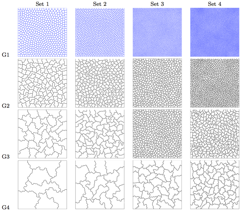
Figure 2: Sequences of agglomerated grids employed for numerical simulations. Top line: fine grids consisting of 512 (Set 1), 1024 (Set 2), 2048 (Set 3) and 4096 (Set 4) polygonal elements.

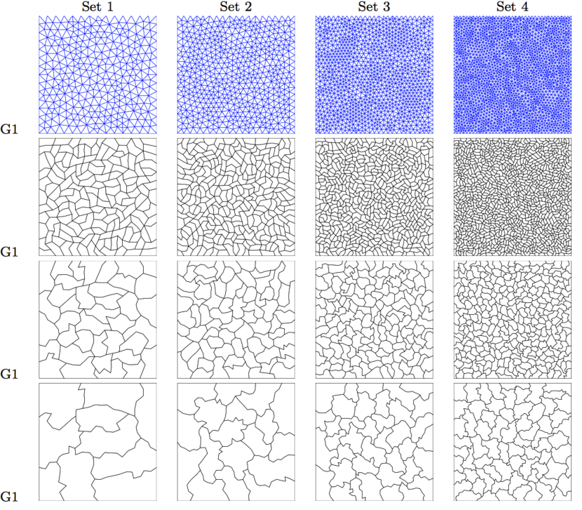
Figure 3: Sequences of agglomerated grids employed for numerical simulations. Top line: fine grids consisting of 582 (Set 1), 1086 (Set 2), 2198 (Set 3) and 4318 (Set 4) triangular elements.

Before testing the performance of the two-level and W-cycle multigrid solvers presented in Algorithm 1 and Algorithm 2, respectively, we first address the issue of the choice of the penalization coefficient $C_{\sigma}^{j}$ in (2.2). According to Lemma 2, the bilinear form $\mathcal{A}_{j}(\cdot,\cdot)$ is coercive provided that $C_{\sigma}^{j}$ is chosen large enough. In Table 1, we report the coercivity constant ${\color[rgb]{0,0,0}\mathsf{C}_{\mathsf{coer}}}$ of (12) for a fixed value of $C_{\sigma}^{j}\equiv C_{\sigma}=10$ for $j=1,\ldots,4$. We observe that the bilinear form is uniformly coercive for a constant value of the penalization coefficient, which is of the same magnitude as the one typically employed on standard shape-regular triangular meshes. As a consequence, in the following, we set $C_{\sigma}^{j}\equiv C_{\sigma}=10$ for $j=1,\dots,4$.

	Set 1	Set 2	Set 3	Set 4
G1	0.7385	0.7375	0.7370	0.7364
G2	0.7624	0.7564	0.7559	0.7545
G3	0.7827	0.7818	0.7720	0.7611
G4	0.8153	0.8054	0.8001	0.7827

Table 1: Value of the coercivity constant ${\color[rgb]{0,0,0}\mathsf{C}_{\mathsf{coer}}}$ for the sets of grids considered in Figure 2 with $C_{\sigma}^{j}=C_{\sigma}=10$, $j=1,\dots$,4.

We now consider the sequence of the grids shown in Figure 2, Set 1, and numerically evaluate the constant ${\color[rgb]{0,0,0}\mathsf{C}_{\mathsf{2lvl}}}\Sigma_{J}$, $J=2$, in Theorem 4.1 and the constant ${\color[rgb]{0,0,0}\widehat{\mathsf{C}}}\Sigma_{3}$ in Theorem 4.2, for the $h$-version of the two solvers, based on selecting $m_{1}=m_{2}=m=2p^{2}$, cf. Figure 4. Here, we observe that ${\color[rgb]{0,0,0}\mathsf{C}_{\mathsf{2lvl}}}\Sigma_{2}$ and ${\color[rgb]{0,0,0}\widehat{\mathsf{C}}}\Sigma_{3}$ are roughly (asymptotically) constant, as the polynomial degree $p$ increases; thereby, this implies that ${\color[rgb]{0,0,0}\widetilde{\mathsf{C}}_{J,J-1}}$, $J=2,3$, respectively, is approximately $\mathcal{O}(1)$, as $p$ increases. Notice also that, in practice, the parameter $\mu=0$, even whenever a $p$–optimal interpolant cannot be explicetely constructed.

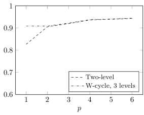
Figure 4: Estimates of ${\color[rgb]{0,0,0}\mathsf{C}_{\mathsf{2lvl}}}\Sigma_{J}$ and ${\color[rgb]{0,0,0}\widehat{\mathsf{C}}}\Sigma_{3}$ in (44) and (52), respectively, as a function of $p$, and $m_{1}=m_{2}=m=2p^{2}$. Sequence of agglomerated meshes shown in Figure 2, Set 1.

Next, we investigate the performance of the two-level and W-cycle multigrid schemes in terms of the convergence factor

$$\rho=\exp\left(\frac{1}{N}\ln\frac{\|\mathbf{r}_{N}\|_{2}}{\|\mathbf{r}_{0}\|_{2}}\right),$$

where $N$ denotes the number of iterations required to attain convergence up to a (relative) tolerance of $10^{-8}$ and $\mathbf{r}_{N}$ and $\mathbf{r}_{0}$ are the final and initial residual vectors, respectively. In Table 2, we report the iteration counts and the convergence factor (in parenthesis), needed to attain convergence of the $h$-version of the two-level (TL) method and W-cycle multigrid scheme (with 3 and 4 levels), as a function of the number of elements (given by the choice of different grid sets), and the number of smoothing steps ($m_{1}=m_{2}=m$). Here, we have fixed the polynomial approximation order on each level $p_{j}\equiv p=1$. We first observe that, although the agglomerated grids, in general, do not necessarily strictly satisfy Assumption 2.2, the number of iterations, for fixed $m$, does not significantly increase with the number of elements in the underlying mesh; moreover, for the W-cycle solver, the number of iterations remains bounded with the number of levels. As expected, the convergence is faster for larger values of $m$ and the solvers are convergent provided the number of smoothing steps is sufficiently large. For each grid, we have also reported the iteration counts ${\color[rgb]{0,0,0}\mathsf{N}_{\mathsf{it}}^{\mathsf{CG}}}$ for the Conjugate Gradient (CG) method, which shows that the two proposed solvers outperform the CG scheme in terms of the number of iterations required to attain convergence, even when a small number of smoothing steps are employed. For the sake of comparison, we also report the iteration counts ${\color[rgb]{0,0,0}\mathsf{N}_{\mathsf{it}}^{\mathsf{PCG}}}$ for the Preconditioned Conjugate Gradient (PCG) method, based on employing a simple block Jacobi preconditioner. The extension to polytopic grids of the domain decomposition preconditioning techniques, such as, for example, the ones proposed in AntHou ; AntHouSme ; AntSarVerZik_2016 , in the DG setting, or in Pav94 ; SchoMelPecZag_2008 , in the conforming setting, are currently under investigation and will be the subject of future research. Table 3 presents analogous results for the first three sets of meshes, in the case when $p=3$. Here, we observe that, as expected, the convergence factor increases, but the increase in $p$ does not require an increase in the minimal number of smoothing steps needed to ensure that the underlying multilevel solvers are convergent.

	Set 1			Set 2
	TL	W-cycle		TL	W-cycle
		3 lvl	4 lvl		3 lvl	4 lvl
$m=3$	133 (0.87)	160 (0.89)	167 (0.90)	121 (0.86)	191 (0.91)	188 (0.91)
$m=5$	95 (0.82)	113 (0.85)	113 (0.85)	88 (0.81)	121 (0.86)	125 (0.86)
$m=8$	72 (0.77)	82 (0.80)	81 (0.80)	67 (0.76)	86 (0.81)	88 (0.81)
$m=12$	57 (0.72)	63 (0.74)	62 (0.74)	54 (0.71)	65 (0.75)	67 (0.76)
$m=16$	49 (0.68)	52 (0.70)	51 (0.69)	46 (0.67)	55 (0.71)	56 (0.72)
$m=20$	44 (0.65)	45 (0.66)	44 (0.66)	40 (0.63)	48 (0.68)	49 (0.68)
	${\color[rgb]{0,0,0}\mathsf{N}_{\mathsf{it}}^{\mathsf{CG}}}=445$, ${\color[rgb]{0,0,0}\mathsf{N}_{\mathsf{it}}^{\mathsf{PCG}}}=326$			${\color[rgb]{0,0,0}\mathsf{N}_{\mathsf{it}}^{\mathsf{CG}}}=633$, ${\color[rgb]{0,0,0}\mathsf{N}_{\mathsf{it}}^{\mathsf{PCG}}}=480$
	Set 3			Set 4
	TL	W-cycle		TL	W-cycle
		3 lvl	4 lvl		3 lvl	4 lvl
$m=3$	140 (0.88)	188 (0.91)	192 (0.91)	162 (0.89)	198 (0.91)	198 (0.91)
$m=5$	99 (0.83)	124 (0.86)	128 (0.87)	112 (0.85)	131 (0.87)	131 (0.87)
$m=8$	74 (0.78)	89 (0.81)	91 (0.82)	83 (0.80)	94 (0.82)	94 (0.82)
$m=12$	58 (0.73)	68 (0.76)	69 (0.76)	65 (0.75)	73 (0.77)	72 (0.77)
$m=16$	49 (0.68)	56 (0.72)	57 (0.72)	55 (0.71)	61 (0.74)	61 (0.74)
$m=20$	43 (0.65)	48 (0.68)	49 (0.68)	49 (0.68)	53 (0.71)	53 (0.70)
	${\color[rgb]{0,0,0}\mathsf{N}_{\mathsf{it}}^{\mathsf{CG}}}=946$, ${\color[rgb]{0,0,0}\mathsf{N}_{\mathsf{it}}^{\mathsf{PCG}}}=678$			${\color[rgb]{0,0,0}\mathsf{N}_{\mathsf{it}}^{\mathsf{CG}}}=1234$, ${\color[rgb]{0,0,0}\mathsf{N}_{\mathsf{it}}^{\mathsf{PCG}}}=958$

Table 2: Iteration counts and converge factor (in parenthesis) of the $h$-version of the two-level and W-cycle solvers and iteration counts of the CG/PCG methods as a function of $m$ ($C_{\sigma}^{j}\equiv C_{\sigma}=10$, $p=1$). Sequences of agglomerated meshes shown in Figure 2.

	Set 1			Set 2			Set 3
	TL	W-cycle		TL	W-cycle		TL	W-cycle
		3 lvl	4 lvl		3 lvl	4 lvl		3 lvl	4 lvl
$m=3$	1281	1334	1342	1168	1272	1362	1230	1379	1391
$m=5$	816	832	839	737	790	844	774	852	860
$m=8$	546	551	561	487	517	551	513	555	557
$m=12$	388	394	400	343	363	385	362	387	384
$m=16$	305	312	316	268	284	299	284	301	296
$m=20$	254	261	263	222	235	246	235	249	242
	${\color[rgb]{0,0,0}\mathsf{N}_{\mathsf{it}}^{\mathsf{CG}}}=1954$, ${\color[rgb]{0,0,0}\mathsf{N}_{\mathsf{it}}^{\mathsf{PCG}}}=885$			${\color[rgb]{0,0,0}\mathsf{N}_{\mathsf{it}}^{\mathsf{CG}}}=2809$, ${\color[rgb]{0,0,0}\mathsf{N}_{\mathsf{it}}^{\mathsf{PCG}}}=1264$			${\color[rgb]{0,0,0}\mathsf{N}_{\mathsf{it}}^{\mathsf{CG}}}=4174$, ${\color[rgb]{0,0,0}\mathsf{N}_{\mathsf{it}}^{\mathsf{PCG}}}=1708$

Table 3: Iteration counts of the $h$-version of the two-level and W-cycle solvers as a function of $m$ and the number of levels and iteration counts of the CG/PCG methods ($C_{\sigma}^{j}\equiv C_{\sigma}=10$, $p=3$). Sequences of agglomerated meshes shown in Figure 2.

Next, we consider the sets of nested grids obtained by agglomerating the shape-regular triangular meshes shown in Figure 3, first row. The initial triangular decompositions constist of 528 (Set 1), 1086 (Set 2), 2198 (Set 3) and 4318 (Set 4) elements, cf. Figure 3, first row. In Table 4, we show the iteration counts needed to attain convergence with respect to a fixed tolerance of $10^{-8}$ as a function of the set (i.e., the number of elements) and the number of smoothing steps of the $h$-version of the two-level and W-cycle multigrid solvers, with $p_{j}=p=1$. We recall that, as in the previous numerical test, we have considered $C_{\sigma}^{j}\equiv C_{\sigma}=10$, for each $j$. The results are similar to the case of initial polygonal meshes, with uniform convergence with respect to the granularity of the mesh and, in the case of the W-cycle solver, also with respect to the number of levels. We again attain improved performance, compared to the standard CG and PCG methods, in terms of the number of iterations required to attain convergence.

	Set 1			Set 2
	TL	W-cycle		TL	W-cycle
		3 lvl	4 lvl		3 lvl	4 lvl
$m=4$	246 (0.90)	258 (0.90)	262 (0.90)	282 (0.89)	291 (0.90)	292 (0.90)
$m=6$	177 (0.87)	185 (0.87)	188 (0.87)	199 (0.86)	205 (0.87)	204 (0.87)
$m=10$	120 (0.81)	125 (0.82)	127 (0.82)	133 (0.81)	136 (0.82)	136 (0.82)
$m=14$	94 (0.77)	98 (0.78)	99 (0.78)	104 (0.77)	106 (0.78)	106 (0.78)
$m=18$	79 (0.74)	82 (0.74)	83 (0.74)	87 (0.74)	89 (0.75)	89 (0.75)
	${\color[rgb]{0,0,0}\mathsf{N}_{\mathsf{it}}^{\mathsf{CG}}}=551$, ${\color[rgb]{0,0,0}\mathsf{N}_{\mathsf{it}}^{\mathsf{PCG}}}=369$			${\color[rgb]{0,0,0}\mathsf{N}_{\mathsf{it}}^{\mathsf{CG}}}=771$, ${\color[rgb]{0,0,0}\mathsf{N}_{\mathsf{it}}^{\mathsf{PCG}}}=504$
	Set 3			Set 4
	TL	W-cycle		TL	W-cycle
		3 lvl	4 lvl		3 lvl	4 lvl
$m=4$	328 (0.90)	333 (0.91)	329 (0.90)	421 (0.91)	425 (0.91)	422 (0.91)
$m=6$	231 (0.87)	234 (0.88)	232 (0.87)	292 (0.88)	293 (0.89)	292 (0.89)
$m=10$	153 (0.82)	154 (0.83)	153 (0.82)	190 (0.83)	191 (0.84)	189 (0.84)
$m=14$	118 (0.78)	119 (0.79)	118 (0.78)	145 (0.79)	148 (0.80)	146 (0.80)
$m=18$	98 (0.75)	99 (0.75)	98 (0.75)	120 (0.76)	123 (0.77)	122 (0.77)
	${\color[rgb]{0,0,0}\mathsf{N}_{\mathsf{it}}^{\mathsf{CG}}}=1145$, ${\color[rgb]{0,0,0}\mathsf{N}_{\mathsf{it}}^{\mathsf{PCG}}}=718$			${\color[rgb]{0,0,0}\mathsf{N}_{\mathsf{it}}^{\mathsf{CG}}}=1630$, ${\color[rgb]{0,0,0}\mathsf{N}_{\mathsf{it}}^{\mathsf{PCG}}}=974$

Table 4: Iteration counts and converge factor (in parenthesis) of the $h$-version of the two-level and W-cycle solvers and iteration counts of the CG and PCG methods as a function of $m$ ($C_{\sigma}^{j}\equiv C_{\sigma}=10$, $p=1$). Sequences of agglomerated meshes shown in Figure 3.

Finally, we present a more exhaustive investigation of the effect of increasing $p$ while keeping fixed the number of smoothing steps. For this set of experiments, we consider a fine grid of 1024 elements and the corresponding agglomerated meshes (Set 2 in Figure 2). In Table 5 we report the iteration counts of the $h$-version of the two-level and W-cycle solvers as a function of $p$, employing $m=5$ pre- and post- smoothing steps. We observe that, as expected, even though both multilevel solvers converge for a fixed value of $m$, the number of iterations required to reduce the relative residual below the given tolerance grows with increasing $p$. However, the two-level and W-cycle multigrid solvers still employ less iterations, than the number required by both the CG and PCG methods, cf. the last two columns of Table 5.

	TL	W-cycle		${\color[rgb]{0,0,0}\mathsf{N}_{\mathsf{it}}^{\mathsf{CG}}}$	${\color[rgb]{0,0,0}\mathsf{N}_{\mathsf{it}}^{\mathsf{PCG}}}$
		3 lvl	4 lvl
$p=1$	88	121	125	633	480
$p=2$	357	434	443	1701	953
$p=3$	737	790	844	2809	1264
$p=4$	958	1093	1184	4574	1821
$p=5$	876	1096	1201	6796	2213

Table 5: Iteration counts of the $h$-version of the two-level and W-cycle solvers as a function of $p$ and the number of levels and corresponding CG/PCG iteration counts ($C_{\sigma}^{j}\equiv C_{\sigma}=10$, $m=5$). Sequence of agglomerated meshes shown in Figure 2, Set 2.

As a numerical comparison, we have solved the correspoding linear systems of equations employing an unsmoothed aggregation Algebraic Multigrid (AMG) algorithm based on three popular algebraic agglomeration strategies. More precisely, in the considered AMG methods the agglomerates are formed, at a purely algebraic level, by using either the maximal independent set, the (approximate) maximum weighted matching or the greedy aggregation algorithms, and the resulting coarse levels are then employed as before within a $W$-cycle iteration with a Richardon smoother with $m=5$ pre- and post-smoothing steps. In Table 6 we report, for each of the considered agglomeration strategies, the number of agglomeration levels (N. levels), as well as the computed convergence factors $\rho$. As it is clear from the results reported in Table 6, classical algebraic agglomeration procedures are not efficient when applied to the matrices arising from high-order DG approximations; indeed in all the cases the resulting algorithm is not able to reduce the (relative) residual below the given tolerance within 5000 iterations, cf. last column of Table 6 where the iteration counts (${\color[rgb]{0,0,0}\mathsf{N}_{\mathsf{it}}^{\mathsf{AMG}}}$) are shown. Such behaviour strongly suggests that the geometric information needs to be taken into account in the construction of the solver and/or more sophisticated (aggressive) aggregation-based algebraic algorithms, as well as Schwarz-type smoothers, such as the ones proposed, for example, in OlsonSchroder_2011 ; BastianBlattScheichl_2012 , should be considered. Such developments are currently under investigation and will be the subject of future research.

	Max. independent set		Max. weighted matching		Greedy aggregation
	${\color[rgb]{0,0,0}\rho}$	N. levels	${\color[rgb]{0,0,0}\rho}$	N. levels	${\color[rgb]{0,0,0}\rho}$	N. levels	${\color[rgb]{0,0,0}\mathsf{N}_{\mathsf{it}}^{\mathsf{AMG}}}$
$p=1$	0.9990	3	0.9987	7	0.9992	5	$>$ 5000
$p=2$	0.9989	3	0.9986	8	0.9988	5	$>$ 5000
$p=3$	0.9989	3	0.9986	8	0.9990	6	$>$ 5000
$p=4$	0.9989	3	0.9986	9	0.9989	6	$>$ 5000
$p=5$	0.9989	3	0.9986	9	0.9988	6	$>$ 5000

Table 6: Number of agglomeration levels (N. levels) and computed convergce factors ($\rho$) of Algebraic $W$-cycle multigrid method (Richardon smoother, $m=5$ pre- and post-smoothing steps) as a function of $p$. The agglomerates are formed algebraically by using either the maximal independent set, the (approximate) maximum weighted matching or the greedy aggregation algorithms. The initial fine grid is shown in Figure 2, Set 2 (first row).

7 Conclusions

We have presented and analyzed two-level and multigrid schemes for the efficient solution of the linear system of equations arising from the $hp$-version of the interior penalty DG scheme on polygonal/polyhedral meshes. The attractive feature of the proposed algorithms is that the auxiliary sequence of meshes needed by the multilevel solver can be generated by a (successive) general geometric agglomeration procedure starting from an initial grid made of (possibly arbitrarily-shaped) elements. Such an approach fully exploits the flexibilty of DG methods in terms of their ability to handle arbitrarily-shaped elements, including polytopic elements, see AntBreMar09 ; dg_cfes_2012 ; Canetal14 ; BasBotColSub ; CangianiDongGeorgoulisHouston_2016 ; AntFacRusVer2016 ; CangianiDongGeorgoulis_2016 , and the recent review paper Anetal16_review . Extending the theoretical results recently presented in AntSarVer15 on quasi-uniform meshes, we have proved that, under mild geometric assumptions on the quality of the agglomerates, both the two-level and W-cycle multigrid schemes converge uniformly with respect to the discretization parameters (namely, the granularity of the underlying partition and the polynomial approximation degree $p$) and, for the multigrid scheme, the number of levels, provided that the number of smoothing steps is chosen sufficiently large. We have also demonstrated through numerical experiments that the theoretical assumption concerning the need to employ a sufficently large number of smoothing steps is not needed in practice, i.e., our algorithms converge even if the number of smoothing steps is kept fixed independently of the polynomial approximation degree $p$. However, in this latter case, the performance of the iterative solvers deteriorates, as expected, when increasing $p$.

References

• (1) P. F. Antonietti, L. Beirão Da Veiga, D. Mora, and M. Verani. A stream virtual element formulation of the Stokes problem on polygonal meshes. SIAM Journal on Numerical Analysis, 52(1):386–404, 2014.
• (2) P. F. Antonietti, L. Beirão Da Veiga, S. Scacchi, and M. Verani. A C1 virtual element method for the Cahn-Hilliard equation with polygonal meshes. SIAM Journal on Numerical Analysis, 54(1):34–56, 2016.
• (3) P. F. Antonietti, F. Brezzi, and L. D. Marini. Bubble stabilization of discontinuous Galerkin methods. Comput. Methods Appl. Mech. Engrg., 198(21-26):1651–1659, 2009.
• (4) P. F. Antonietti, A. Cangiani, J. Collins, Z. Dong, E. Georgoulis, S. Giani, and P. Houston. Review of discontinuous Galerkin finite element methods for partial differential equations on complicated domains. G.R. Barrenechea, F. Brezzi, A. Cangiani, A., E.H. Georgoulis (eds.), Building Bridges: Connections and Challenges in Modern Approaches to Numerical Partial Differential Equations, Lecture Notes in Computational Science and Engineering 114, 2016, DOI 10.1007/978-3-319-41640-3-9.
• (5) P. F. Antonietti, C. Facciola, A. Russo, and M. Verani. Discontinuous Galerkin approximation of flows in fractured porous media. Technical Report 22/2016, MOX Report, 2016.
• (6) P. F. Antonietti, L. Formaggia, A. Scotti, M. Verani, and V. Nicola. Mimetic finite difference approximation of flows in fractured porous media. M2AN Math. Model. Numer. Anal., 50(3):809–832, 2016.
• (7) P. F. Antonietti, S. Giani, and P. Houston. $hp$–Version composite discontinuous Galerkin methods for elliptic problems on complicated domains. SIAM J. Sci. Comput., 35(3):A1417–A1439, 2013.
• (8) P. F. Antonietti, S. Giani, and P. Houston. Domain decomposition preconditioners for Discontinuous Galerkin methods for elliptic problems on complicated domains. J. Sci. Comput., 60(1):203–227, 2014.
• (9) P. F. Antonietti and P. Houston. A class of domain decomposition preconditioners for $hp$-discontinuous Galerkin finite element methods. J. Sci. Comput., 46(1):124–149, 2011.
• (10) P. F. Antonietti and P. Houston. Preconditioning high-order discontinuous Galerkin discretizations of elliptic problems. Lecture Notes in Computational Science and Engineering, 91:231–238, 2013.
• (11) P. F. Antonietti, P. Houston, and I. Smears. A note on optimal spectral bounds for nonoverlapping domain decomposition preconditioners for hp-version discontinuous Galerkin methods. International Journal of Numerical Analysis and Modeling, 13(4):513–524, 2016.
• (12) P. F. Antonietti, M. Sarti, and M. Verani. Multigrid algorithms for $hp$-discontinuous Galerkin discretizations of elliptic problems. SIAM J. Numer. Anal., 53(1):598–618, 2015.
• (13) P. F. Antonietti, M. Sarti, and M. Verani. Multigrid algorithms for high order discontinuous Galerkin methods. Lecture Notes in Computational Science and Engineering, 104:3–13, 2016.
• (14) P. F. Antonietti, M. Sarti, M. Verani, and L. Zikatanov. A uniform additive Schwarz preconditioner for high-order Discontinuous Galerkin approximations of elliptic problems. J. Sci. Comput., 2016, doi:10.1007/s10915-016-0259-9.
• (15) D. N. Arnold. An interior penalty finite element method with discontinuous elements. SIAM J. Numer. Anal., 19(4):742–760, 1982.
• (16) D. N. Arnold, F. Brezzi, B. Cockburn, and L. D. Marini. Unified analysis of discontinuous Galerkin methods for elliptic problems. SIAM J. Numer. Anal., 39(5):1749–1779, 2001/2002.
• (17) J. Aubin. Approximation des problèmes aux limites non homogènes pour des opérateurs non linéaires. J. Math. Anal. Appl., 30:510–521, 1970.
• (18) I. Babuška. The finite element method with penalty. Math. Comp., 27(122):221–228, 1973.
• (19) G. A. Baker. Finite element methods for elliptic equations using nonconforming elements. Math. Comp., 31(137):45–59, 1977.
• (20) F. Bassi, L. Botti, A. Colombo, F. Brezzi, and G. Manzini. Agglomeration-based physical frame dg discretizations: An attempt to be mesh free. Math. Models Methods Appl. Sci., 24(8):1495–1539, 2014.
• (21) F. Bassi, L. Botti, A. Colombo, D. A. Di Pietro, and P. Tesini. On the flexibility of agglomeration based physical space discontinuous Galerkin discretizations. J. Comput. Phys., 231(1):45–65, 2012.
• (22) F. Bassi, L. Botti, A. Colombo, and S. Rebay. Agglomeration based discontinuous Galerkin discretization of the Euler and Navier-Stokes equations. Comput. & Fluids, 61:77–85, 2012.
• (23) P. Bastian, M. Blatt, and R. Scheichl. Algebraic multigrid for discontinuous Galerkin discretizations of heterogeneous elliptic problems. Numer. Linear Algebra Appl., 19(2):367–388, 2012.
• (24) L. Beirão Da Veiga, F. Brezzi, A. Cangiani, G. Manzini, L. D. Marini, and A. Russo. Basic principles of virtual element methods. Mathematical Models and Methods in Applied Sciences, 23(01):199–214, 2013.
• (25) L. Beirão Da Veiga, F. Brezzi, L. Marini, and A. Russo. Mixed virtual element methods for general second order elliptic problems on polygonal meshes. ESAIM: Mathematical Modelling and Numerical Analysis, 50(3):727–747, 2016.
• (26) L. Beirão Da Veiga, F. Brezzi, L. Marini, and A. Russo. Virtual element method for general second-order elliptic problems on polygonal meshes. Mathematical Models and Methods in Applied Sciences, 26(4):729–750, 2016.
• (27) L. Beirão da Veiga, K. Lipnikov, and G. Manzini. The mimetic finite difference method for elliptic problems, volume 11 of MS&A. Modeling, Simulation and Applications. Springer, Cham, 2014.
• (28) J. Bramble. Multigrid Methods. Number 294 in Pitman Research Notes in Mathematics Series. Longman Scientific & Technical, Harlow, UK, 1993.
• (29) F. Brezzi, K. Lipnikov, and M. Shashkov. Convergence of the mimetic finite difference method for diffusion problems on polyhedral meshes. SIAM J. Numer. Anal., 43(5):1872–1896 (electronic), 2005.
• (30) F. Brezzi, K. Lipnikov, and M. Shashkov. Convergence of mimetic finite difference method for diffusion problems on polyhedral meshes with curved faces. Math. Models Methods Appl. Sci., 16(2):275–297, 2006.
• (31) F. Brezzi, K. Lipnikov, and V. Simoncini. A family of mimetic finite difference methods on polygonal and polyhedral meshes. Math. Models Methods Appl. Sci., 15(10):1533–1551, 2005.
• (32) A. Cangiani, Z. Dong, and E. Georgoulis. $hp$-Version space-time discontinuous Galerkin methods for parabolic problems on prismatic meshes. Submitted for publication, 2016.
• (33) A. Cangiani, Z. Dong, E. Georgoulis, and P. Houston. $hp$–Version discontinuous Galerkin methods on polygonal and polyhedral meshes. 2016, in preparation.
• (34) A. Cangiani, Z. Dong, E. Georgoulis, and P. Houston. $hp$-Version discontinuous Galerkin methods for advection-diffusion-reaction problems on polytopic meshes. M2AN Math. Model. Numer. Anal., 50(3):699–725, 2016.
• (35) A. Cangiani, E. H. Georgoulis, and P. Houston. $hp$-Version discontinuous Galerkin methods on polygonal and polyhedral meshes. Math. Models Methods Appl. Sci., 24(10):2009–2041, 2014.
• (36) T. F. Chan, J. Xu, and L. Zikatanov. An agglomeration multigrid method for unstructured grids. In Domain decomposition methods, 10 (Boulder, CO, 1997), volume 218 of Contemp. Math., pages 67–81. Amer. Math. Soc., Providence, RI, 1998.
• (37) B. Cockburn, G. E. Karniadakis, and C.-W. Shu, editors. Discontinuous Galerkin methods, Springer-Verlag, Berlin, 2000. Theory, computation and applications. Papers from the 1st International Symposium held in Newport, RI, May 24-26, 1999.
• (38) D. A. Di Pietro and A. Ern. Mathematical aspects of discontinuous Galerkin methods, volume 69 of Mathématiques & Applications (Berlin) [Mathematics & Applications]. Springer, Heidelberg, 2012.
• (39) T.-P. Fries and T. Belytschko. The extended/generalized finite element method: An overview of the method and its applications. International Journal for Numerical Methods in Engineering, 84(3):253–304, 2010.
• (40) E. H. Georgoulis. Inverse-type estimates on $hp$-finite element spaces and applications. Math. Comp., 77(261):201–219 (electronic), 2008.
• (41) W. Hackbusch. Multi-grid methods and applications, volume 4 of Springer series in computational mathematics. Springer, Berlin, 1985.
• (42) W. Hackbusch and S. Sauter. Composite finite elements for problems containing small geometric details. Part II: Implementation and numerical results. Comput. Visual Sci., 1(4):15–25, 1997.
• (43) W. Hackbusch and S. Sauter. Composite finite elements for the approximation of PDEs on domains with complicated micro-structures. Numer. Math., 75(4):447–472, 1997.
• (44) J. S. Hesthaven and T. Warburton. Nodal Discontinuous Galerkin Methods: Algorithms, Analysis, and Applications. Springer Publishing Company, Incorporated, 1st edition, 2007.
• (45) J. Hyman, M. Shashkov, and S. Steinberg. The numerical solution of diffusion problems in strongly heterogeneous non-isotropic materials. J. Comput. Phys., 132(1):130–148, 1997.
• (46) J.-L. Lions. Problèmes aux limites non homogènes à donées irrégulières: Une méthode d’approximation. In Numerical Analysis of Partial Differential Equations (C.I.M.E. 2 Ciclo, Ispra, 1967), Edizioni Cremonese, Rome, pages 283–292. 1968.
• (47) I. Moulitsas and G. Karypis. Mgridgen/Parmgridgen Serial/Parallel Library for Generating Coarse Grids for Multigrid Methods. University of Minnesota, Department of Computer Science/Army HPC Research Center, 2001. Available at: www-users.cs.umn.edu/~moulitsa/software.html.
• (48) I. Moulitsas and G. Karypis. Multilevel algorithms for generating coarse grids for multigrid methods,. In Supercomputing 2001 Conference Proceedings, 2001.
• (49) J. Nitsche. Über ein Variationsprinzip zur Lösung von Dirichlet Problemen bei Verwendung von Teilräumen, die keinen Randbedingungen unterworfen sind. Abh. Math. Sem. Uni. Hamburg, 36:9–15, 1971.
• (50) L. N. Olson and J. B. Schroder. Smoothed aggregation multigrid solvers for high-order discontinuous Galerkin methods for elliptic problems. J. Comput. Phys., 230(18):6959–6976, 2011.
• (51) L. F. Pavarino. Additive Schwarz methods for the $p$-version finite element method. Numer. Math., 66(4):493–515, 1994.
• (52) W. Reed and T. Hill. Triangular mesh methods for the neutron transport equation. Technical Report LA-UR-73-479, Los Alamos Scientific Laboratory, 1973.
• (53) B. Rivière. Discontinuous Galerkin methods for solving elliptic and parabolic equations, volume 35 of Frontiers in Applied Mathematics. Society for Industrial and Applied Mathematics (SIAM), Philadelphia, PA, 2008. Theory and implementation.
• (54) J. Schöberl, J. M. Melenk, C. Pechstein, and S. Zaglmayr. Additive Schwarz preconditioning for $p$-version triangular and tetrahedral finite elements. IMA J. Numer. Anal., 28(1):1–24, 2008.
• (55) C. Schwab. $p$- and $hp$-finite element methods. Numerical Mathematics and Scientific Computation. The Clarendon Press, Oxford University Press, New York, 1998. Theory and applications in solid and fluid mechanics.
• (56) E. Stein. Singular Integrals and Differentiability Properties of Functions. Princeton, University Press, Princeton, N.J., 1970.
• (57) N. Sukumar and A. Tabarraei. Conforming polygonal finite elements. International Journal for Numerical Methods in Engineering, 61(12):2045–2066, 2004.
• (58) A. Tabarraei and N. Sukumar. Extended finite element method on polygonal and quadtree meshes. Computer Methods in Applied Mechanics and Engineering, 197(5):425–438, 2008.
• (59) C. Talischi, G. Paulino, A. Pereira, and I. Menezes. Polymesher: A general-purpose mesh generator for polygonal elements written in matlab. Structural and Multidisciplinary Optimization, 45(3):309–328, 2012.
• (60) M. F. Wheeler. An elliptic collocation-finite element method with interior penalties. SIAM J. Numer. Anal., 15(1):152–161, 1978.