Approximate Lifted Inference with Probabilistic Databases

Abstract

This paper proposes a new approach for approximate evaluation of #P-hard queries with probabilistic databases. In our approach, every query is evaluated entirely in the database engine by evaluating a fixed number of query plans, each providing an upper bound on the true probability, then taking their minimum. We provide an algorithm that takes into account important schema information to enumerate only the minimal necessary plans among all possible plans. Importantly, this algorithm is a strict generalization of all known results of PTIME self-join-free conjunctive queries: A query is safe if and only if our algorithm returns one single plan. We also apply three relational query optimization techniques to evaluate all minimal safe plans very fast. We give a detailed experimental evaluation of our approach and, in the process, provide a new way of thinking about the value of probabilistic methods over non-probabilistic methods for ranking query answers.

1 Introduction

Probabilistic inference over large data sets is becoming a central data management problem. Recent large knowledge bases, such as Yago [27], Nell [5], DeepDive [9], or Google’s Knowledge Vault [14], have millions to billions of uncertain tuples. Data sets with missing values are often “completed” using inference in graphical models [6, 52] or sophisticated low rank matrix factorization techniques [15, 51], which ultimately results in a large, probabilistic database. Data sets that use crowdsourcing are also uncertain [1]. And, very recently, probabilistic databases have been applied to bootstrapping over samples of data [55].

However, probabilistic inference is known to be #P-hard in the size of the database, even for some very simple queries [7]. Today’s state of the art inference engines use either sampling-based methods or are based on some variant of the DPLL algorithm for Weighted Model Counting. For example, Tuffy [36], a popular implementation of Markov Logic Networks (MLN) over relational databases, uses Markov Chain Monte Carlo methods (MCMC). Gibbs sampling can be significantly improved by adapting some classical relational optimization techniques [56]. For another example, MayBMS [3] and its successor Sprout [39] use query plans to guide a DPLL-based algorithm for Weighted Model Counting [25]. While both approaches deploy some advanced relational optimization techniques, at their core they are based on general purpose probabilistic inference techniques, which either run in exponential time (DPLL-based algorithms have been proven recently to take exponential time even for queries computable in polynomial time [4]), or require many iterations until convergence.

In this paper, we propose a different approach to query evaluation with probabilistic databases. In our approach, every query is evaluated entirely in the database engine. Probability computation is done at query time, using simple arithmetic operations and aggregates. Thus, probabilistic inference is entirely reduced to a standard query evaluation problem with aggregates. There are no iterations and no exponential blowups. All benefits of relational engines (such as cost-based optimizations, multi-core query processing, shared-nothing parallelization) are directly available to queries over probabilistic databases. To achieve this, we compute approximate rather than exact probabilities, with a one-sided guarantee: The probabilities are guaranteed to be upper bounds to the true probabilities, which we show is sufficient to rank the top query answers with high precision. Our approach consists of approximating the true query probability by evaluating a fixed number of “safe queries” (the number depends on the query), each providing an upper bound on the true probability, then taking their minimum.

We briefly review “safe queries,” which are queries whose data complexity is in PTIME. They can be evaluated using safe query plans [7, 17, 53], which are related to a technique called lifted inference in the AI literature [12, 28]; the entire computation is pushed inside the database engine and is thus efficient. For example, the query $q_{1}(z){\,:\!\!-\,}R(z,x),S(x,y),K(x,y)$ has the safe query plan $P_{1}=\pi_{z}(R\Join_{x}(\pi_{x}(S\Join_{x,y}K)))$, where every join operator multiplies the probabilities, and every projection with duplicate elimination treats probabilistic events as independent. The literature describes several classes of safe queries [8, 17] and shows that they can be evaluated very efficiently. However, most queries are “unsafe:” They are provably #P-hard and do not admit safe plans.

In this paper, we prove that every conjunctive query without self-joins can be approximated by a fixed number of safe queries, called “safe dissociations” of the original query. Every safe dissociation is guaranteed to return an upper bound on the true probability and can be evaluated in PTIME data complexity. The number of safe dissociations depends only on the query and not the data. Moreover, we show how to find “minimal safe dissociations” which are sufficient to find the best approximation to the given query. For example, the unsafe query $q_{2}(z){\,:\!\!-\,}R(z,x),S(x,y),T(y)$ has two minimal safe dissociations, $q_{2}^{\prime}(z){\,:\!\!-\,}R(z,x),S(x,y),T^{\prime}(x,y)$ and $q_{2}^{\prime\prime}(z){\,:\!\!-\,}R^{\prime}(z,x,y),S(x,y),T(y)$. Both queries are safe and, by setting the probability of every tuple $R^{\prime}(z,x,y)$ equal to that of $R(z,x)$ and similarly for $T^{\prime}$, they return an upper bound for the probabilities of each answer tuple from $q_{2}(z)$. One benefit of our approach is that, if the query happens to be safe, then it has a unique minimal safe dissociation, and our algorithm finds it.

Contributions. (1) We show that there exists a 1-to-1 correspondence between the safe dissociations of a self-join-free conjunctive query and its query plans. One simple consequence is that every query plan computes an upper bound of the true probability. For example, the two safe dissociations above correspond to the plans $P_{2}^{\prime}=\pi_{z}(R\Join_{x}(\pi_{x}(S\Join_{x,y}T)))$, and $P_{2}^{\prime\prime}=\pi_{z}((\pi_{zy}(R\Join_{x}S))\Join_{y}T)$. We give an intuitive system R-style algorithm [48] for enumerating all minimal safe dissociations of a query $q$. Our algorithm takes into account important schema-level information: functional dependencies and whether a relation is deterministic or probabilistic. We prove that our algorithm has several desirable properties that make it a strict generalization of previous algorithms described in the literature: If $q$ is safe then the algorithm returns only one safe plan that computes $q$ exactly; and if $q$ happens to be safe on the particular database instance (e.g., the data happens to satisfy a functional dependency), then one of the minimal safe dissociations will compute the query exactly. (2) We use relational optimization techniques to compute all minimal safe dissociations of a query efficiently in the database engine. Some queries may have a large number of dissociations; e.g., a 8-chain query has 4279 safe dissociations, of which 429 are minimal. Computing 429 queries sequentially in the database engine would still be prohibitively expensive. Instead, we tailor three relational query optimization techniques to dissociation: ($i$) combining all minimal plans into one single query, ($ii$) reusing common subexpressions with views, and ($iii$) performing deterministic semi-join reductions. (3) We conduct an experimental validation of our technique, showing that, with all our optimizations enabled, computing hard queries over probabilistic databases incurs only a modest penalty over computing the same query on a deterministic database: For example, the 8-chain query runs only a factor of $<10$ slower than on a deterministic database. We also show that the dissociation-based technique has high precision for ranking query answers based on their output probabilities.

In summary, our three main contributions are:

1. We describe an efficient algorithm for finding all minimal safe dissociations for self-join-free conjunctive queries in the presence of schema knowledge. If the query is safe, then our algorithm returns a single minimal plan, which is the safe plan for the query (Section 3).

2. We show how to apply three traditional query optimization techniques to dramatically improve the performance of the dissociation (Section 4).

3. We perform a detailed experimental validation of our approach, showing both its effectiveness in terms of query performance, and the quality of returned rankings. Our experiments also include a novel comparison between deterministic and probabilistic ranking approaches (Section 5).

All proofs for this submission together with additional illustrating examples are available in our technical report on arXiv [21].

2 Background

Probabilistic Databases. We fix a relational vocabulary $\sigma=(R_{1},\ldots,R_{m})$. A probabilistic database $D$ is a database plus a function $p(t)\in[0,1]$ associating a probability to each tuple $t\in D$. A possible world is a subset of $D$ generated by independently including each tuple $t$ in the world with probability $p(t)$. Thus, the database $D$ is tuple-independent. We use bold notation (e.g., $\bm{\mathbf{x}}$) to denote sets or tuples. A self-join-free conjunctive query is a first-order formula $q(\bm{\mathbf{y}})=\exists x_{1}\ldots\exists x_{k}.(a_{1}\wedge\ldots\wedge a_{m})$ where each atom $a_{i}$ represents a relation $R_{i}(\bm{\mathbf{x}}_{i})$, the variables $x_{1},\ldots,x_{k}$ are called existential variables, and $\bm{\mathbf{y}}$ are called the head variables (or free variables). The term “self-join-free” means that the atoms refer to distinct relational symbols. We assume therefore w.l.o.g. that every relational symbol $R_{1},\ldots,R_{m}$ occurs exactly once in the query. Unless otherwise stated, a query in this paper denotes a self-join-free conjunctive query. As usual, we abbreviate the query by $q(\bm{\mathbf{y}}){\,:\!\!-\,}a_{1},\ldots,a_{m}$, and write $\textup{{HVar}}(q)=\bm{\mathbf{y}}$, $\textup{{EVar}}(q)=\{x_{1},\ldots,x_{k}\}$ and $\textup{{Var}}(q)=\textup{{HVar}}(q)\cup\textup{{EVar}}(q)$ for the set of head variables, existential variables, and all variables of $q$. If $\textup{{HVar}}(q)=\emptyset$ then $q$ is called a Boolean query. We also write $\textup{{Var}}(a_{i})$ for the variables in atom $a_{i}$ and $\and(x)$ for the set of atoms that contain variable $x$. The active domain of a variable $x_{i}$ is denoted ${\mathit{ADom}}_{x_{i}}$, and the active domain of the entire database is ${\mathit{ADom}}=\bigcup_{i}{\mathit{ADom}}_{x_{i}}$. The focus of probabilistic query evaluation is to compute ${{\mathbb{P}}}\!\left(q\right)$; i.e. the probability that the query is true in a randomly chosen world.

Safe queries, safe plans. It is known that the data complexity of any query $q$ is either in PTIME or #P-hard. The former are called safe queries and are characterized precisely by a syntactic property called hierarchical queries [7]. We briefly review these results:

Definition (Hierarchical query)

Query $q$ is called hierarchical iff for any $x,y\in\textup{{EVar}}(q)$, one of the following three conditions hold: $\and(x)\subseteq\and(y)$, $\and(x)\cap\and(y)=\emptyset$, or $\and(x)\supseteq\and(y)$.

For example, the query $q_{1}{\,:\!\!-\,}R(x,y),S(y,z),T(y,z,u)$ is hierarchical, while $q_{2}{\,:\!\!-\,}R(x,y),S(y,z),T(z,u)$ is not, as neither of the three conditions holds for the variables $y$ and $z$.

Theorem 1 (Dichotomy [7])

If $q$ is hierarchical, then ${{\mathbb{P}}}\!\left(q\right)$ can be computed in PTIME in the size of $D$. Otherwise, computing ${{\mathbb{P}}}\!\left(q\right)$ is #P-hard in the size of $D$.

We next give an equivalent, recursive characterization of hierarchical queries, for which we need a few definitions. We write $\textup{{SVar}}(q)$ for the separator variables (or root variables); i.e. the set of existential variables that appear in every atom. $q$ is disconnected if its atoms can be partitioned into two non-empty sets that do not share any existential variables (e.g., $q{\,:\!\!-\,}R(x,y),S(z,u),T(u,v)$ is disconnected and has two connected components: “$R(x,y)$” and “$S(z,u),T(u,v)$”). For every set of variables $\bm{\mathbf{x}}$, denote $q-{\bm{\mathbf{x}}}$ the query obtained by removing all variables $\bm{\mathbf{x}}$ (and decreasing the arities of the relation symbols that contain variables from $\bm{\mathbf{x}}$).

Lemma (Hierarchical queries)

$q$ is hierarchical iff either: (1) $q$ has a single atom; (2) $q$ has $k\geq 2$ connected components all of which are hierarchical; or (3) $q$ has a separator variable $x$ and $q-x$ is hierarchical.

Definition (Query plan)

Let $R_{1},\ldots,R_{m}$ be a relational vocabulary. A query plan $P$ is given by the grammar

$$P::= \,R_{i}(\bm{\mathbf{x}})\,\,\,|\,\,\pi_{\bm{\mathbf{x}}}P\,\,\,|\,\,\!\Join\!\!\big{[}P_{1},\ldots,P_{k}\big{]}$$

where $R_{i}(\bm{\mathbf{x}})$ is a relational atom containing the variables $\bm{\mathbf{x}}$ and constants, $\pi_{\bm{\mathbf{x}}}$ is the project operator with duplicate elimination, and $\Join\!\!\big{[}\ldots\big{]}$ is the natural join in prefix notation, which we allow to be $k$-ary, for $k\geq 2$. We require that joins and projections alternate in a plan. We do not distinguish between join orders, i.e. $\Join\!\!\big{[}P_{1},P_{2}\big{]}$ is the same as $\Join\!\!\big{[}P_{2},P_{1}\big{]}$.

We write $\textup{{HVar}}(P)$ for the head variables of $P$ (defined as the variables $\bm{\mathbf{x}}$ of the top-most projection $\pi_{\bm{\mathbf{x}}}$, or the union of the top-most projections if the last operation is a join). Every plan $P$ represents a query $q_{P}$ defined by taking all atoms mentioned in $P$ and setting $\textup{{HVar}}(q_{P})=\textup{{HVar}}(P)$. For notational convenience, we also use the “project-away” notation, by writing $\pi_{\!-\!\bm{\mathbf{y}}}(P)$ instead of $\pi_{\bm{\mathbf{x}}}(P)$, where $\bm{\mathbf{y}}$ are the variables being projected away; i.e. $\bm{\mathbf{y}}=\textup{{HVar}}(P)-\bm{\mathbf{x}}$.

Given a probabilistic database $D$ and a plan $P$, each output tuple $t\in P(D)$ has a $\textit{score}(t)$, defined inductively on the structure of $P$ as follows: If $t\in R_{i}(\bm{\mathbf{x}})$, then $\textit{score}(t)=p(t)$, i.e. its probability in $D$; if $t\in\,\Join\!\!\big{[}P_{1}(D),\ldots,P_{k}(D)\big{]}$ where $t=\Join\!\!\big{[}t_{1},\ldots,t_{k}\big{]}$, then $\textit{score}(t)=\prod_{i=1}^{k}\textit{score}(t_{i})$; and if $t\in\pi_{\bm{\mathbf{x}}}(P(D))$, and $t_{1},\ldots,t_{n}\in P(D)$ are all the tuples that project into $t$, then $\textit{score}(t)=1-\prod_{i=1}^{n}(1-\textit{score}(t_{i}))$. In other words, score computes a probability by assuming that all tuples joined by $\Join$ are independent, and all duplicates eliminated by $\pi$ are also independent. If these conditions hold, then score is the correct query probability, but in general the score is different from the probability. Therefore, score is not equal to the probability, in general, and is also called an extensional semantics [18, 41]. For a Boolean plan $P$, we get one single score, which we denote $\textit{score}(P)$.

The requirement that joins and projections alternate is w.l.o.g. because nested joins like $\Join\!\!\big{[}\Join\!\!\big{[}R_{1},R_{2}\big{]},R_{3}\big{]}$ can be rewritten into $\Join\!\!\big{[}R_{1},R_{2},R_{3}\big{]}$ while keeping the same probability score. For the same reason we do not distinguish between different join orders.

Definition (Safe plan)

A plan $P$ is called safe iff, for any join operator $\Join^{p}\!\!\big{[}P_{1},\ldots,P_{k}\big{]}$, all subplans have the same head variables: $\textup{{HVar}}(P_{i})=\textup{{HVar}}(P_{j})$ for all $1\leq i,j\leq k$.

The recursive definition of section 2 gives us immediately a safe plan for a hierarchical query. Conversely, every safe plan defines a hierarchical query. The following summarizes our discussion:

Proposition (Safety [7])

(1) Let $P$ be a plan for the query $q$. Then $\textit{score}(P)={{\mathbb{P}}}\!\left(q\right)$ for any probabilistic database iff $P$ is safe. (2) Assuming #P$\neq$PTIME, a query $q$ is safe (i.e. ${{\mathbb{P}}}\!\left(q\right)$ has PTIME data complexity) iff it has a safe plan $P$; in that case the safe plan is unique, and ${{\mathbb{P}}}\!\left(q\right)=\textit{score}(P)$.

Boolean Formulas. Consider a set of Boolean variables $\mathbf{X}=\{X_{1},X_{2},\ldots\}$ and a probability function $p:\mathbf{X}\rightarrow[0,1]$. Given a Boolean formula $F$, denote ${{\mathbb{P}}}\!\left(F\right)$ the probability that $F$ is true if each variable $X_{i}$ is independently true with probability $p(X_{i})$. In general, computing ${{\mathbb{P}}}\!\left(F\right)$ is #P-hard in the number of variables $\mathbf{X}$. If $D$ is a probabilistic database then we interpret every tuple $t\in D$ as a Boolean variable and denote the lineage of a Boolean $q{\,:\!\!-\,}g_{1},\ldots,g_{m}$ on $D$ as the Boolean DNF formula $F_{q,D}=\bigvee_{\theta:\theta\models q}\theta(g_{1})\wedge\cdots\wedge\theta(g_{m})$, where $\theta$ ranges over all assignments of $\textup{{EVar}}(q)$ that satisfy $q$ on $D$. It is well known that ${{\mathbb{P}}}\!\left(q\right)={{\mathbb{P}}}\!\left(F_{q,D}\right)$. In other words the probability of a Boolean query is the same as the probability of its lineage formula.

Example (Lineage)

If $F=XY\vee XZ$ then ${{\mathbb{P}}}\!\left(F\right)=p(1\!-\!(1\!-\!q)(1\!-\!r))=pq+pr-pqr$, where $p=p(X),q=p(Y)$, and $r=p(Z)$. Consider now the query $q{\,:\!\!-\,}R(x),S(x,y)$ over the database $D=\{R(1),R(2),S(1,4),S(1,5)\}$. Then the lineage formula is $F_{q,D}=R(1)\wedge S(1,4)\vee R(1)\wedge S(1,5)$, i.e. same as $F$, up to variable renaming. It is now easy to see that ${{\mathbb{P}}}\!\left(q\right)={{\mathbb{P}}}\!\left(F_{q,D}\right)$.

A key technique that we use in this paper is the following result from [22]: Let $F,F^{\prime}$ be two Boolean formulas with sets of variables $\mathbf{X}$ and $\mathbf{X}^{\prime}$, respectively. We say that $F^{\prime}$ is a dissociation of $F$ if there exists a substitution $\theta:\mathbf{X}^{\prime}\rightarrow\mathbf{X}$ such that $F^{\prime}[\theta]=F$. If $\theta^{-1}(X)=\{X^{\prime},X^{\prime\prime},\ldots\}$ then we say that the variable $X$ dissociates into $X^{\prime},X^{\prime\prime},\ldots$; if $|\theta^{-1}(X)|=1$ then we assume w.l.o.g. that $\theta^{-1}(X)=X$ (up to variable renaming) and we say that $X$ does not dissociate. Given a probability function $p:\mathbf{X}\rightarrow[0,1]$, we extend it to a probability function $p^{\prime}:\mathbf{X}^{\prime}\rightarrow[0,1]$ by setting $p^{\prime}(X^{\prime})=p(\theta(X^{\prime}))$. Then, we have shown:

Theorem 2 (Oblivious DNF bounds [22])

Let $F^{\prime}$ be a monotone DNF formula that is a dissociation of $F$ through the substitution $\theta$. Assume that for any variable $X$, no two distinct dissociations $X^{\prime},X^{\prime\prime}$ of $X$ occur in the same prime implicant of $F^{\prime}$. Then (1) ${{\mathbb{P}}}\!\left(F\right)\leq{{\mathbb{P}}}\!\left(F^{\prime}\right)$, and (2) if all dissociated variables $X\in\mathbf{X}$ are deterministic (meaning: $p(X)=0$ or $p(X)=1$) then ${{\mathbb{P}}}\!\left(F\right)={{\mathbb{P}}}\!\left(F^{\prime}\right)$.

Intuitively, a dissociation $F^{\prime}$ is obtained from a formula $F$ by taking different occurrences of a variable $X$ and replacing them with fresh variables $X^{\prime},X^{\prime\prime},\ldots$; in doing this, the probability of $F^{\prime}$ may be easier to compute, giving us an upper bound for ${{\mathbb{P}}}\!\left(F\right)$.

Example (section 2 cont.)

$F^{\prime}=X^{\prime}Y\vee X^{\prime\prime}Z$ is a dissociation of $F=XY\vee XZ$, and its probability is ${{\mathbb{P}}}\!\left(F^{\prime}\right)=1\!-\!(1\!-\!pq)(1\!-\!pr)=pq+pr-p^{2}qr$. Here, only the variable $X$ dissociates into $X^{\prime},X^{\prime\prime}$. It is easy to see that ${{\mathbb{P}}}\!\left(F\right)\leq{{\mathbb{P}}}\!\left(F^{\prime}\right)$. Moreover, if $p=0$ or 1, then ${{\mathbb{P}}}\!\left(F\right)={{\mathbb{P}}}\!\left(F^{\prime}\right)$. The condition that no two dissociations of the same variable occur in a common prime implicant is necessary: for example, $F^{\prime}=X^{\prime}X^{\prime\prime}$ is a dissociation of $F=X$. However ${{\mathbb{P}}}\!\left(F\right)=p$, ${{\mathbb{P}}}\!\left(F^{\prime}\right)=p^{2}$, and we do not have ${{\mathbb{P}}}\!\left(F\right)\leq{{\mathbb{P}}}\!\left(F^{\prime}\right)$.

3 Dissociation of queries

This section introduces our main technique for approximate query processing. After defining dissociations (Section 3.1), we show that some of them are in 1-to-1 correspondence with query plans, then derive our first algorithm for approximate query processing (Section 3.2). Finally, we describe two extensions in the presence of deterministic relations or functional dependencies (Section 3.3).

3.1 Query dissociation

Definition (Dissociation)

Given a Boolean query $q{\,:\!\!-\,}R_{1}(\bm{\mathbf{x}}_{1}),\ldots,R_{m}(\bm{\mathbf{x}}_{m})$ and a probabilistic database $D$. Let $\Delta=(\bm{\mathbf{y}}_{1},\ldots,\bm{\mathbf{y}}_{m})$ be a collection of sets of variables with $\bm{\mathbf{y}}_{i}\subseteq\textup{{Var}}(q)-\textup{{Var}}(g_{i})$ for every relation $R_{i}$. The dissociation defined by $\Delta$ has then two components:

1. the dissociated query: $q^{\Delta}{\,:\!\!-\,}R_{1}^{\bm{\mathbf{y}}_{1}}(\bm{\mathbf{x}}_{1},\bm{\mathbf{y}}_{1}),\ldots,R_{m}^{\bm{\mathbf{y}}_{m}}(\bm{\mathbf{x}}_{m},\bm{\mathbf{y}}_{m})$, where each $R_{i}^{\bm{\mathbf{y}}_{i}}(\bm{\mathbf{x}}_{i},\bm{\mathbf{y}}_{i})$ is a new relation of arity $|\bm{\mathbf{x}}_{i}|+|\bm{\mathbf{y}}_{i}|$.

2. the dissociated database instance $D^{\Delta}$ consisting of the tables over the vocabulary $\sigma^{\Delta}$ obtained by evaluating (deterministically) the following queries over the instance $D$:

   $$R_{i}^{\bm{\mathbf{y}}_{i}}(\bm{\mathbf{x}}_{i},\bm{\mathbf{y}}_{i}) {\,:\!\!-\,}R_{i}(\bm{\mathbf{x}}_{i}),{\mathit{ADom}}_{y_{i1}}(y_{i1}),\ldots,{\mathit{ADom}}_{y_{ik}}(y_{ik})$$

   where $\bm{\mathbf{y}}_{i}=(y_{i1},\ldots,y_{ik_{i}})$. For each tuple $t^{\prime}\in R_{i}^{\bm{\mathbf{y}}_{i}}$, its probability is defined as $p^{\prime}(t^{\prime})=p(\pi_{\bm{\mathbf{x}}_{i}}(t^{\prime}))$, i.e. the probability of $t$ in the database $D$.

Thus, a dissociation acts on both the query expression and the database instance: It adds some variables $\bm{\mathbf{y}}_{i}$ to each relational symbol $R_{i}$ of the query expression, and it computes a new instance for each relation $R_{i}^{\bm{\mathbf{y}}_{i}}$ by copying every record $t\in R_{i}$ once for every tuple in the cartesian product ${\mathit{ADom}}_{y_{i1}}\times\cdots\times{\mathit{ADom}}_{y_{ik}}$. When $\bm{\mathbf{y}}_{i}=\emptyset$ then we abbreviate $R_{i}^{\emptyset}$ with $R_{i}$. We give a simple example:

Example (section 2 cont.)

Consider $q{\,:\!\!-\,}R(x),S(x,y)$. Then $\Delta=(\{y\},\emptyset)$ defines the following dissociation: $q^{\Delta}=R^{y}(x,y),S(x,y)$, and the new relation $R^{y}$ contains the tuples $R^{y}(1,4),R^{y}(1,5),R^{y}(2,4),R^{y}(2,5)$. Notice that the lineage of the dissociated query $q^{\Delta}$ is $F_{q^{\Delta},D^{\Delta}}=R^{y}(1,4),S(1,4)\vee R^{y}(1,5),S(1,5)$ and is the same (up to variable renaming) as the dissociation of the lineage of query $q$: $F^{\prime}=X^{\prime}Y\vee X^{\prime\prime}Z$.

Theorem 3 (Upper query bounds)

For every dissociation $\Delta$ of $q$: ${{\mathbb{P}}}(q)\leq{{\mathbb{P}}}(q^{\Delta})$.

Proof 3.4.

Theorem 3 follows immediately from Theorem 2 by noting that the lineage $F_{q^{\Delta},D^{\Delta}}$ is a dissociation of the lineage $F_{q,D}$ through the substitution $\theta:D^{\Delta}\rightarrow D$ defined as follows: for every tuple $t^{\prime}\in R_{i}^{\bm{\mathbf{y}}_{i}}$, $\theta(t^{\prime})=\pi_{\bm{\mathbf{x}}_{i}}(t^{\prime})$.

Definition 3.5 (Safe dissociation).

A dissociation $\Delta$ of a query $q$ is called safe if the dissociated query ${q^{\Delta}}$ is safe.

By Theorem 1, a dissociation is safe (i.e. its probability can be evaluated in PTIME) iff $q^{\Delta}$ is hierarchical. Hence, amongst all dissociations, we are interested in those that are easy to evaluate and use them as a technique to approximate the probabilities of queries that are hard to compute. The idea is simple: Find a safe dissociation $\Delta$, compute ${{\mathbb{P}}}\!\left(q^{\Delta}\right)$, and thereby obtain an upper bound on ${{\mathbb{P}}}\!\left(q\right)$. In fact, we will consider all safe dissociations and take the minimum of their probabilities, since this gives an even better upper bound on ${{\mathbb{P}}}\!\left(q\right)$ than that given by a single dissociation. We call this quantity the propagation score of the query $q$.

Definition 3.6 (Propagation).

The propagation score $\rho(q)$ for a query $q$ is the minimum score of all safe dissociations: $\rho(q)=\min_{\Delta}{{\mathbb{P}}}(q^{\Delta})$ with $\Delta$ ranging over all safe dissociations.

The difficulty in computing $\rho(q)$ is the number of dissociations that is large even for relatively small queries: If $q$ has $k$ existential variables and $m$ atoms, then $q$ has $2^{|K|}$ possible dissociations with $K=\sum_{i=1}^{m}\big{(}k-|\texttt{Var}(g_{i})|\big{)}$ forming a partial order in the shape of a power set lattice (see Fig.​ 1a). Therefore, our next step is to prune the space of dissociations and to examine only the minimum number necessary. We start by defining a partial order on dissociations:

Definition 3.7 (Partial dissociation order).

We define the partial order on the dissociations of a query as:

$$\Delta\preceq\Delta^{\prime}\,\,\Leftrightarrow\,\,\forall i:\bm{\mathbf{y}}_{i}\subseteq\bm{\mathbf{y}}_{i}^{\prime}$$

Whenever $\Delta\preceq\Delta^{\prime}$, then $q^{\Delta^{\prime}},D^{\Delta^{\prime}}$ is a dissociation of $q^{\Delta},D^{\Delta}$ (given by $\Delta^{\prime\prime}=\Delta^{\prime}-\Delta$). Therefore, we obtain immediately:

Corollary 3.8 (Partial dissociation order).

If $\Delta\preceq\Delta^{\prime}$ then ${{\mathbb{P}}}(q^{\Delta})\leq{{\mathbb{P}}}(q^{\Delta^{\prime}})$.

Example 3.9 (Partial dissociation order).

Consider the query $q{\,:\!\!-\,}R(x),S(x),T(x,y),U(y)$. It is unsafe and allows $2^{3}=8$ dissociations which are shown in Fig.​ 1a with the help of an “augmented incidence matrix”: each row represents one relation and each column one variable: An empty circle ($\circ$) indicates that a relation contains a variable; a full circle ($\bullet$) indicates that a relation is dissociated on a variable (the reason for using two separate symbols becomes clear when we later include domain knowledge). Among those 8 dissociations, 5 are safe, shaded in green, and have the hierarchy among variables highlighted. Furthermore, 2 of the 5 safe dissociations are minimal: $q^{\Delta_{3}}{\,:\!\!-\,}R(x),S(x),T(x,y),U^{x}(x,y)$, and $q^{\Delta_{4}}{\,:\!\!-\,}R^{y}(x,y),S^{y}(x,y),T(x,y),U(y)$ . To illustrate that these dissociations are upper bounds, consider a database with $R=T=U=\{1,2\}$, $S=\{(1,1),(1,2),(2,2)\}$, and the probability of all tuples $=\frac{1}{2}$. Then $q$ has probability $\frac{83}{2^{9}}\approx 0.161$, while $q^{\Delta_{3}}$ has probability $\frac{169}{2^{10}}\approx 0.165$, and $q^{\Delta_{4}}$ has probability $\frac{353}{2^{11}}\approx 0.172$, both of which are upper bounds. The propagation score is the minimum score of all minimal safe dissociations and thus $\approx 0.165$.  $\blacksquare$

(a)

(b)

Figure 1: Example 3.9 (a): Partial dissociation order for $q{\,:\!\!-\,}R(x),S(x),$ $T(x,y),U(y)$. Safe dissociations are green and have the hierarchies between variables shown (3 to 7), minimal safe dissociations are dark green and double-lined (3 and 4). (b): All 5 query plans for $q$ and their correspondence to safe dissociations (3 to 7).

In general, the set of dissociations forms a lattice, with the smallest element $\Delta_{\bot}=(\emptyset,\ldots,\emptyset)$ ($q^{\Delta_{\bot}}=q$) and the largest element $\Delta_{\top}=(\textup{{Var}}(q)-\textup{{Var}}(g_{1}),\ldots,\textup{{Var}}(q)-\textup{{Var}}(g_{m}))$ ($q^{\Delta_{\top}}$ is safe, since every atom contains all variables). As we move up in the lattice the probability increases, but the safe/unsafe status may toggle arbitrarily from safe to unsafe and back. For example $q{\,:\!\!-\,}R(x),S(x),T(y)$ is safe, its dissociation $q^{\prime}{\,:\!\!-\,}R(x),S^{y}(x,y),T(y)$ is unsafe, yet the next dissociation $q^{\prime\prime}{\,:\!\!-\,}R(x),S^{y}(x,y),T^{x}(x,y)$ is safe again.

This suggests the following naive algorithm for computing $\rho(q)$: Enumerate all dissociations $\Delta_{1},\Delta_{2},\ldots$ by traversing the lattice breadth-first, bottom up (i.e. whenever $\Delta_{i}\prec\Delta_{j}$ then $i<j$). For each dissociation $\Delta_{i}$, check if $q^{\Delta_{i}}$ is safe. If so, then first update $\rho\leftarrow\min(\rho,{{\mathbb{P}}}(q^{\Delta_{i}}))$, then remove from the list all dissociations $\Delta_{j}\succ\Delta_{i}$. However, this algorithm is inefficient for practical purposes for two reasons: ($i$) we need to iterate over many dissociations in order to discover those that are safe; and ($ii$) computing ${{\mathbb{P}}}(q^{\Delta_{i}})$ requires computing a new database instance $D^{\Delta_{i}}$ for each safe dissociation $\Delta_{i}$. We show in the next section how to avoid both sources of inefficiency by exploiting the lattice structure and by iterating over query plans instead of safe dissociations.

3.2 Dissociations and Plans

We prove here that the safe dissociations $q^{\Delta}$ are in 1-to-1 correspondence with query plans of the original query $q$. This allows us to ($i$) efficiently find safe dissociations (by iterating over query plans instead of all dissociations), and to ($ii$) compute ${{\mathbb{P}}}(q^{\Delta})$ without having to materialize the dissociated database $D^{\Delta}$.

We next describe the 1-to-1 mapping. Consider a safe dissociation $q^{\Delta}$ and denote its corresponding unique safe plan $P^{\Delta}$. This plan uses dissociated relations, hence each relation $R^{\bm{\mathbf{y}}_{i}}_{i}(\bm{\mathbf{x}}_{i},\bm{\mathbf{y}}_{i})$ has extraneous variables $\bm{\mathbf{y}}_{i}$. Drop all variables $\bm{\mathbf{y}}_{i}$ from the relations and all operators using them: This transforms $P^{\Delta}$ into a regular, generally unsafe plan $P$ for $q$. For a trivial example, the plan corresponding to the top dissociation $\Delta_{\top}$ of a query $q$ is $\pi_{\!-\!\textup{{Var}}(q)}(\Join\!\!\big{[}P_{1},\ldots,P_{k}\big{]})$: It performs all joins first, followed by all projections.

Conversely, consider any plan $P$ for $q$. We define its corresponding safe dissociation $\Delta^{P}$ as follows. For each join operation $\Join^{p}\!\!\big{[}P_{1},\ldots,P_{k}\big{]}$, let its join variables JVar be the union of the head variables of all subplans: $\textup{{JVar}}=\bigcup_{j}\textup{{HVar}}(P_{j})$. For every relation $R_{i}$ occurring in $P_{j}$, add the missing variables $\textup{{JVar}}-\textup{{HVar}}(P_{j})$ to $\bm{\mathbf{y}}_{i}$. For example, consider $\Join^{p}\!\!\big{[}R(x),T(x,y),U(y)\big{]}$ (this is the lower join in query plan 5 of Fig.​ 1b). Here, $\textup{{JVar}}=\{x,y\}$, and the corresponding safe dissociation of this subplan is $q^{\Delta}(x,y){\,:\!\!-\,}R^{y}(x,y),T(x,y),U^{x}(x,y)$. Note that while there is a one-to-one mapping between safe dissociations and query plans, unsafe dissociations do not correspond to plans.

Theorem 3.10 (Safe dissociation).

Let $q$ be a conjunctive query without self-joins. (1) The mappings $\Delta\mapsto P^{\Delta}$ and $P\mapsto\Delta^{P}$ are inverses of each other. (2) For every safe dissociation $\Delta$, ${{\mathbb{P}}}(q^{\Delta})=\textit{score}(P^{\Delta})$.

Corollary 3.11 (Upper bounds).

Let $P$ be any plan for a Boolean query $q$. Then ${{\mathbb{P}}}(q)\leq\textit{score}(P)$.

The proof follows immediately from ${{\mathbb{P}}}(q)\leq{{\mathbb{P}}}(q^{\Delta^{P}})$ (Theorem 3) and ${{\mathbb{P}}}(q^{\Delta^{P}})=\textit{score}(P)$ (Theorem 3.10). In other words, any plan for $q$ computes a probability score that is guaranteed to be an upper bound on the correct probability ${{\mathbb{P}}}(q)$.

Theorem 3.10 suggests the following improved algorithm for computing the propagation score $\rho(q)$ of a query: Iterate over all plans $P$, compute their scores, and retain the minimum score $\min_{P}[\textit{score}(P)]$. Each plan $P$ is evaluated directly on the original probabilistic database, and there no need to materialize the dissociated database instance. However, this approach is still inefficient because it computes several plans that correspond to non-minimal dissociations. For example, in Fig.​ 1 plans 5, 6, 7 correspond to non-minimal dissociations, since plan 3 is safe and below them.

Enumerating minimal safe dissociations. Call a plan $P$ minimal if $\Delta^{P}$ is minimal in the set of safe dissociations. For example, in Example 3.9, the minimal plans are 3 and 4. The propagation score is thus the minimum of the scores of the two minimal plans: $\rho(q)=\min_{i\in\{3,4\}}\big{[}\textit{score}\big{(}P^{(i)}\big{)}\big{]}$. Our improved algorithm will iterate only over minimal plans, by relying on a connection between plans and sets of variables that disconnect a query: A cut-set is a set of existential variables $\bm{\mathbf{x}}\in\textup{{EVar}}(q)$ s.t. $q-{\bm{\mathbf{x}}}$ is disconnected. A min-cut-set (for minimal cut-set) is a cut-set for which no strict subset is a cut-set. We denote $\textup{{MinCuts}}(q)$ the set of all min-cut-sets. Note that $q$ is disconnected iff $\textup{{MinCuts}}(q)=\{\emptyset\}$.

The connection between $\textup{{MinCuts}}(q)$ and query plans is given by two observations: (1) Let $P$ be any plan for $q$. If $q$ is connected, then the last operator in $P$ is a projection, i.e.  $P=\pi_{\!-\!\bm{\mathbf{x}}}(\Join\!\!\big{[}P_{1},\ldots,P_{k}\big{]})$, and the projection variables $\bm{\mathbf{x}}$ are the join variables ${\bm{\mathbf{x}}}=\textup{{JVar}}$ because $q$ is Boolean so the plan must project away all variables. We claim that $\bm{\mathbf{x}}$ is a cut-set for $q$ and that $q-{\bm{\mathbf{x}}}$ has $k$ connected components corresponding to $P_{1},\ldots,P_{k}$. Indeed, if $P_{i},P_{j}$ share any common variable $y$, then they must join on $y$, hence $y\in\textup{{JVar}}$. Thus, cut-sets are in 1-to-1 correspondence with the top-most projection operator of a plan. (2) Now suppose that $P$ corresponds to a safe dissociation $\Delta^{P}$, and let $P^{\prime}=\pi_{\!-\!\bm{\mathbf{x}}}(\Join\!\!\big{[}P_{1}^{\prime},\ldots,P_{k}^{\prime}\big{]})$ be its unique safe plan. Then ${\bm{\mathbf{x}}}=\textup{{SVar}}(q^{\Delta^{P}})$; i.e. the top-most project operator removes all separator variables. Furthermore, if $\Delta\succeq\Delta^{P}$ is a larger dissociation, then $\textup{{SVar}}(q^{\Delta})\supseteq\textup{{SVar}}(q^{\Delta^{P}})$ (because any separator variable of a query continues to be a separator variable in any dissociation of that query). Thus, minimal plans correspond to min-cut-sets; in other words, $\textup{{MinCuts}}(q)$ is in 1-to-1 correspondence with the top-most projection operator of minimal plans.

Our discussion leads immediately to Algorithm 1 for computing the propagation score $\rho(q)$. It also applies to non-Boolean queries by treating the head variables as constants, hence ignoring them when computing connected components. The algorithm proceeds recursively. If $q$ is a single atom then it is safe and we return its unique safe plan. If the query has more than one atom, then we consider two cases, when $q-\textup{{HVar}}(q)$ is disconnected or connected. In the first case, every minimal plan is a join, where the subplans are minimal plans of the connected components. In the second case, a minimal plan results from a projection over min-cut-sets. Notice that recursive calls of the algorithm will alternate between these two cases, until they reach a single atom.

Recursive algorithm: MP (EnumerateMinimalPlans)

Input: Query $q(\bm{\mathbf{x}}){\,:\!\!-\,}R_{1}(\bm{\mathbf{x}}_{1}),\ldots,R_{m}(\bm{\mathbf{x}}_{m})$

Output: Set of all minimal query plans $\mathcal{P}$

1 if $m=1$ then $\mathcal{P}\leftarrow\{\pi_{\bm{\mathbf{x}}}R_{1}(\bm{\mathbf{x}}_{1})\}$

2 else

3    Set $\mathcal{P}\leftarrow\emptyset$

4    if $q$ is disconnected then

5       Let $q=q_{1},\ldots,q_{k}$ be the connected components of $q-\textup{{HVar}}(q)$

6       foreach $q_{i}$ do Let $\textup{{HVar}}(q_{i})\leftarrow\textup{{HVar}}(q)\cap\textup{{Var}}(q_{i})$

7       foreach $(P_{1},\ldots,P_{k})\in\textnormal{{MP}}(q_{1})\times\cdots\times\textnormal{{MP}}(q_{k})$ do

8          $\mathcal{P}\leftarrow\mathcal{P}\cup\{\Join^{p}\!\!\big{[}P_{1},\ldots,P_{k}\big{]}\}$

9         

10      

11    else

12       foreach $\bm{\mathbf{y}}\in\textup{{MinCuts}}(q-\textup{{HVar}}(q))$  do

13          Let $q^{\prime}\leftarrow q$ with $\textup{{HVar}}(q^{\prime})\leftarrow\textup{{HVar}}(q)\cup\bm{\mathbf{y}}$

14          foreach $P\in\textnormal{{MP}}(q^{\prime})$ do  $\mathcal{P}\leftarrow\mathcal{P}\cup\{\pi_{\!-\!\bm{\mathbf{y}}}\,P\}$

15         

16      

17   

Algorithm 1 generates all minimal query plans for a given query $q$.

Theorem 3.12 (Algorithm 1).

Algorithm 1 computes the set of all minimal query plans.

Conservativity. Some probabilistic database systems first check if a query $q$ is safe, and in that case compute the exact probability using the safe plan, otherwise use some approximation technique. We show that Algorithm 1 is conservative, in the sense that, if $q$ is safe, then $\rho(q)={{\mathbb{P}}}\!\left(q\right)$. Indeed, in that case $\textnormal{{MP}}(q)$ returns a single plan, namely the safe $P$ for $q$, because the empty dissociation, $\Delta_{\bot}=(\emptyset,\ldots,\emptyset)$, is safe, and it is the bottom of the dissociation lattice, making it the unique minimal safe dissociation.

Score Quality. We show here that the approximation of ${{\mathbb{P}}}\!\left(q\right)$ by $\rho(q)$ becomes tighter as the input probabilities in $D$ decrease. Thus, the smaller the probabilities in the database, the closer does the ranking based on the propagation score approximate the ranking by the actual probabilities.

Proposition 3.13 (Small probabilities).

Given a query $q$ and database $D$. Consider the operation of scaling down the probabilities of all tuples in $D$ with a factor $f<1$. Then the relative error of approximation of ${{\mathbb{P}}}(q)$ by the propagation score $\rho(q)$ decreases as $f$ goes to 0: $\lim_{f\rightarrow 0}\frac{\rho(q)-{{\mathbb{P}}}(q)}{{{\mathbb{P}}}(q)}\rightarrow 0$.

Number of Dissociations. While the number of minimal safe dissociations is exponential in the size of the query, recall that it is independent of the size of the database. Fig.​ 2 gives an overview of the number of minimal query plans, total query plans, and all dissociations for $k$-star and $k$-chain queries (which are later used in Section 5). Later Section 4 gives optimizations that allow us to evaluate a large number of plans efficiently.

$k$-star query				$k$-chain query
$k$	#MP	#P	$\#\Delta$	$k$	#MP	#P	$\#\Delta$
$1$	$1$	$1$	$1$	$2$	$1$	$1$	$1$
$2$	$2$	$3$	$4$	$3$	$2$	$3$	$4$
$3$	$6$	$13$	$64$	$4$	$5$	$11$	$64$
$4$	$24$	$75$	$4096$	$5$	$14$	$45$	$4096$
$5$	$120$	$541$	$>10^{6}$	$6$	$42$	$197$	$>10^{6}$
$6$	$720$	$4683$	$>10^{9}$	$7$	$132$	$903$	$>10^{9}$
$7$	$5040$	$47293$	$>10^{12}$	$8$	$429$	$4279$	$>10^{12}$
seq	$k!$	$\href http://oeis.org/classic/A000670$	$2^{k(k\!-\!1)}$	seq	$\href http://oeis.org/classic/A000108$	$\href http://oeis.org/classic/A001003$	$2^{(k\!+\!1)k}$

Figure 2: Number of minimal plans, total plans, and total dissociations for star and chain queries (A are OEIS sequence numbers [37]).

3.3 Minimal plans with schema knowledge

Next, we show how knowledge of deterministic relations (i.e. all tuples have probability $=1$), and functional dependencies can reduce the number of plans needed to calculate the propagation score.

3.3.1 Deterministic relations (DRs)

Notice that we can treat deterministic relations (DRs) just like probabilistic relations, and 3.11 with ${{\mathbb{P}}}\!\left(q\right)\leq score(P)$ still holds for any plan $P$. Just as before, our goal is to find a minimum number of plans that compute the minimal score of all plans: $\rho(q)=min_{P}score(P)$. It is known that an unsafe query $q$ can become safe (i.e., ${{\mathbb{P}}}\!\left(q\right)$ can be calculated in PTIME with one single plan) if we consider DRs. Thus, in particular, we would still like an improved algorithm that returns one single plan if a query with DRs is safe. The following lemma will help us achieve this goal:

Lemma 3.14 (Dissociation and DRs).

Dissociating a deterministic relation does not change the probability.

Proof 3.15.

Lemma 3.14 follows immediately from Theorem 2 (2) and noting that dissociating tuples in DRs corresponds exactly to dissociating variables $\bm{\mathbf{X}}$ with $p{(X_{i})}=1$.

We thus define a new probabilistic dissociation preorder $\preceq^{p}$ by:

$$\Delta\preceq^{p}\Delta^{\prime}\Leftrightarrow\forall i,R_{i}\mbox{ probabilistic}:{\bm{\mathbf{y}}}_{i}\subseteq{\bm{\mathbf{y}}}_{i}^{\prime}$$

In other words, $\Delta\preceq^{p}\Delta^{\prime}$ still implies ${{\mathbb{P}}}(q^{\Delta})\leq{{\mathbb{P}}}(q^{\Delta^{\prime}})$, but $\preceq^{p}$ is defined on probabilistic relations only. Notice, that for queries without DRs, the relations $\preceq^{p}$ and $\preceq$ coincide. However, for queries with DRs, $\preceq^{p}$ is a preorder, not an order. Therefore, there exist distinct dissociations $\Delta$, $\Delta^{\prime}$ that are equivalent under $\preceq^{p}$ (written as $\Delta\equiv^{p}\Delta^{\prime}$), and thus have the same probability: ${{\mathbb{P}}}(q^{\Delta})={{\mathbb{P}}}(q^{\Delta^{\prime}})$. As a consequence, using $\preceq^{p}$ instead of $\preceq$, allows us to further reduce the number of minimal safe dissociations.

Example 3.16 (DRs).

Consider $q{\,:\!\!-\,}R(x),S(x,y),T^{d}(y)$ where a $d$-exponent indicates a DR. This query is known to be safe. We thus expect our definition of $\rho(q)$ to find that $\rho(q)={{\mathbb{P}}}\!\left(q\right)$. Ignore that $T^{d}$ is deterministic, then $\preceq$ has two minimal plans: $q^{\Delta_{1}}{\,:\!\!-\,}R^{y}(x,y),S(x,y),T^{d}(y)$, and $q^{\Delta_{2}}{\,:\!\!-\,}R(x),S(x,y),T^{dx}(x,y)$. Since $\Delta_{2}$ dissociates only $T^{d}$, we now know from Lemma 3.14 that ${{\mathbb{P}}}\!\left(q\right)={{\mathbb{P}}}\!\left(q^{\Delta_{2}}\right)$. Thus, by using $\preceq$ as before, we still get the correct answer. However, evaluating the plan $P^{\Delta_{1}}$ is always unnecessary since $\Delta_{2}\preceq^{p}\Delta_{1}$. In contrast, without information about DRs, $\Delta_{2}\not\preceq^{p}\Delta_{1}$, and we would thus have to evaluate both plans.

Fig.​ 3 illustrates this with augmented incidence matrices: dissociated variables in DRs are now marked with empty circles ($\circ$) instead of full circles ($\bullet$), and the preorder $\preceq^{p}$ is determined entirely by full circles (representing dissociated variables in probabilistic relations). However, as before, the correspondence to plans (as implied by the hierarchy between all variables) is still determined by empty and full circles. Fig.​ 3b shows that $\rho(q)={{\mathbb{P}}}\!\left(q^{\Delta_{2}}\right)={{\mathbb{P}}}\!\left(q\right)$ since $\Delta_{0}\equiv^{p}\Delta_{2}\preceq^{p}\Delta_{1}\equiv\Delta_{3}$. Thus, the query is safe, and it suffices to evaluate only $P^{\Delta_{2}}$. Notice that $q$ is not hierarchical, but still safe since it is in an equivalence class with a query that is hierarchical: $\Delta_{0}\equiv^{p}\Delta_{2}$. Fig.​ 3c shows that, with $R^{d}$ and $T^{d}$ being deterministic, all three possible query plans (corresponding to $\Delta_{1}$, $\Delta_{2}$, and $\Delta_{3}$) form a “minimal equivalence class” in $\preceq^{p}$ with $\Delta^{0}$, and thus give the exact probability. We, therefore, want to modify our algorithm to return just one plan from each “minimal safe equivalence class.” Ideally, we prefer the plan corresponding to $\Delta_{3}$ (or more generally, the top plan in $\preceq$ for each minimum equivalence class) since $P^{\Delta_{3}}$ least constrains the join order between tables.

(a)

(b) $T^{d}$

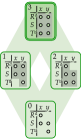
(c) $R^{d}$ and $T^{d}$

Figure 3: Example 3.16: The presence of DRs $R^{d}$ and $T^{d}$ in (b) and (c) changes the original partial dissociation order for $q{\,:\!\!-\,}R(x),S(x,y),T(y)$ in (a): Several dissociations now have the same probability (shown with shaded areas instead of arrows). Our modified algorithm now returns, for each minimal safe equivalence class, the query plan for the top most dissociation (shown in dark green and double-lined).

We now explain two simple modifications to Algorithm 1 that achieve exactly our desired optimizations described above:

1. Denote with $\textup{{MinPCuts}}(q)$ the set of minimal cut-sets that disconnect the query into at least two connected components with probabilistic tables. Replace $\textup{{MinCuts}}(q)$ in Algorithm 1 with $\textup{{MinPCuts}}(q)$.

2. Denote with $m_{p}$ the number of probabilistic relations in a query. Replace the stopping condition in Algorithm 1 with: if $m^{p}\leq 1$ then $\mathcal{P}\leftarrow\{\pi_{\bm{\mathbf{x}}}\Join^{p}\!\!\big{[}R_{1}(\bm{\mathbf{x}}_{1}),\ldots,R_{m}(\bm{\mathbf{x}}_{m})\big{]}\}$. In other words, if a query has maximal one probabilistic relation, than join all relations followed by projecting on the head variables.

Theorem 3.17 (Algorithm 1 with DRs).

Algorithm 1 with above 2 modifications returns a minimum number of plans to calculate $\rho(q)$ given schema knowledge about DRs.

For example, for $q{\,:\!\!-\,}R(x),S(x,y),T^{d}(y)$, $\textup{{MinCuts}}(q)=\{\{x\},\{y\}\}$, while $\textup{{MinPCuts}}(q)=\{\{x\}\}$. Therefore, the modified algorithm returns $P^{\Delta_{2}}$ as single plan. For $q{\,:\!\!-\,}R^{d}(x),S(x,y),T^{d}(y)$, the stopping condition is reached (also, $\textup{{MinPCuts}}(q)=\{\emptyset\}$) and the algorithm returns $P^{\Delta_{3}}$ as single plan (see Fig.​ 3c).

3.3.2 Functional dependencies (FDs)

Knowledge of functional dependencies (FDs), such as keys, can also restrict the number of necessary minimal plans. A well known example is the query $q{\,:\!\!-\,}R(x),S(x,y),T(y)$ from Example 3.16; it becomes safe if we know that $S$ satisfies the FD $\Gamma:x\rightarrow y$ and has a unique safe plan that corresponds to dissociation $\Delta_{2}$. In other words, we would like our modified algorithm to take $\Gamma$ into account and to not return the plan corresponding to dissociation $\Delta_{1}$.

Let $\bm{\Upgamma}$ be the set of FDs on $\textup{{Var}}(q)$ consisting of the union of FDs on every atom $R_{i}$ in $q$. As usual, denote ${\bm{\mathbf{x}}}_{i}^{+}$ the closure of a set of attributes ${\bm{\mathbf{x}}}_{i}$, and denote $\Delta_{\bm{\Upgamma}}=({\bm{\mathbf{y}}}_{1},\ldots,{\bm{\mathbf{y}}}_{m})$ the dissociation defined as follows: for every atom $R_{i}({\bm{\mathbf{x}}}_{i})$ in $q$, ${\bm{\mathbf{y}}}_{i}={\bm{\mathbf{x}}}_{i}^{+}\setminus{\bm{\mathbf{x}}}_{i}$. Then we show:

Lemma 3.18 (Dissociation and FDs).

Dissociating a table $R_{i}$ on any variable $y\in{\bm{\mathbf{x}}}_{i}^{+}$ does not change the probability.

This lemma is similar to Lemma 3.14. We can thus further refine our probabilistic dissociation preorder ${{\preceq^{p}}^{\prime}}$ by:

$$\Delta{\preceq^{p}}^{\prime}\Delta\Leftrightarrow\forall i,R_{i}\mbox{ probabilistic}:{\bm{\mathbf{y}}}_{i}\setminus\bm{\mathbf{x}}_{i}^{+}\subseteq{\bm{\mathbf{y}}}_{i}^{\prime}\setminus\bm{\mathbf{x}}^{+}_{i}$$

As a consequence, using ${\preceq^{p}}^{\prime}$ instead of $\preceq^{p}$, allows us to further reduce the number of minimal safe equivalence classes. We next state a result by [39] in our notation:

Proposition 3.19 (Safety and FDs [39, Prop. IV.5]).

A query $q$ is safe iff $q^{\Delta_{\bm{\Upgamma}}}$ is hierarchical.

This justifies our third modification to Algorithm 1 for computing $\rho(q)$ of a query $q$ over a database that satisfies $\bm{\Upgamma}$: First compute ${\Delta_{\bm{\Upgamma}}}$, then run $q^{\Delta_{\bm{\Upgamma}}}$ on our previously modified Algorithm 1.

Theorem 3.20 (Algorithm 1 with FDs).

Algorithm 1 with above 3 modifications returns a minimum number of plans to calculate $\rho(q)$ given schema knowledge about DRs and FDs.

It is easy to see that our modified algorithm returns one single plan iff the query is safe, taking into account its structure, DRs and FDs. It is thus a strict generalization of all known safe self-join-free conjunctive queries [7, 39]. In particular, we can reformulate the known safe query dichotomy [7] in our notation very succinctly:

Corollary 3.21 (Dichotomy).

${{\mathbb{P}}}\!\left(q\right)$ can be calculated in PTIME iff there exists a dissociation $\Delta$ of $q$ that is ($i$) hierarchical, and ($ii$) in an equivalence class with $q$ under ${\preceq^{p}}^{\prime}$.

To see what the corollary says, assume first that there are no FDs: Then $q$ is in PTIME iff there exists a dissociation $\Delta$ of the DRs only, such that $q^{\Delta}$ is hierarchical. If there are FDs, then we first compute the full dissociation $\Delta_{\bm{\Upgamma}}$ (called “full chase” in [39]), then apply the same criterion to $q^{\Delta_{\bm{\Upgamma}}}$.

4 Multi-query Optimizations

So far, Algorithm 1 enumerates all minimal query plans. We then take the minimum score of those plans in order to calculate the propagation score $\rho(q)$. In this section, we develop three optimizations that can considerably reduce the necessary calculations for evaluating all minimal query plans. Note that these three optimizations and the two optimizations from the previous section are orthogonal and can be arbitrarily combined in the obvious way. We use the following example to illustrate the first two optimizations.

Example 4.22 (Optimizations).

Consider $q{\,:\!\!-\,}$ $R(x,z),S(y,u),$ $T(z),U(u),M(x,y,z,u)$. Our default is to evaluate all 6 minimal plans returned by Algorithm 1, then take the minimum score (shown in Fig. 4a). Figure 4b and Fig. 4c illustrate the optimized evaluations after applying Opt. 1, or Opt. 1 and Opt. 2, respectively.  $\blacksquare$

4.1 Opt. 1: One single query plan

Our first optimization creates one single query plan by pushing the min-operator down into the leaves. It thus avoids calculations when it is clear that other calculations must have lower bounds. The idea is simple: Instead of creating one query subplan for each top set $\bm{\mathbf{y}}\in\textup{{MinCuts}}(q)$ in Algorithm 1 of Algorithm 1, the adapted Algorithm 2 takes the minimum score over those top sets, for each tuple of the head variables in Algorithm 2. It thus creates one single query plan.

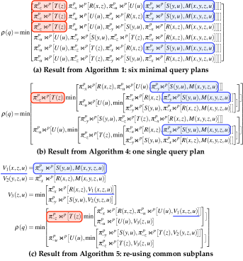
Figure 4: Example 4.22 before and after applying optimizations 1 and 2.

1

Recursive algorithm: SP (SinglePlan)

Input: Query $q(\bm{\mathbf{x}}){\,:\!\!-\,}R_{1}(\bm{\mathbf{x}}_{1}),\ldots,R_{m}(\bm{\mathbf{x}}_{m})$

Output: Single query plan $P$

2

3if $m=1$ then $P\leftarrow\pi^{p}_{\bm{\mathbf{x}}}R_{i}(\bm{\mathbf{x}}_{i})$

4 else

5    if $q$ is disconnected then

6       Let $q=q_{1},\ldots,q_{k}$ be the components connected by $\textup{{EVar}}(q)$

7       Let $\textup{{HVar}}(q_{i})\leftarrow\textup{{HVar}}(q)\cap\textup{{Var}}(q_{i})$

8       $P\leftarrow\Join^{p}\!\!\big{[}\textnormal{{SP}}(q_{1}),\ldots,\textnormal{{SP}}(q_{k})\big{]}$

9      

10    else

11       Let $\textup{{MinCuts}}(q)=\{\bm{\mathbf{y}}_{1},\ldots,\bm{\mathbf{y}}_{j}\}$

12       Let $q^{\prime}_{i}\leftarrow q_{i}$ with $\textup{{HVar}}(q^{\prime}_{i})\leftarrow\textup{{HVar}}(q)\cup\bm{\mathbf{y}}_{i}$

13       if $j\!=\!1$ then $P\leftarrow\pi^{p}_{\!-\!\bm{\mathbf{y}}_{1}}\textnormal{{SP}}(q_{1}^{\prime})$

14       else $P\leftarrow\min\!\left[\pi^{p}_{\!-\!\bm{\mathbf{y}}_{1}}\textnormal{{SP}}(q_{1}^{\prime}),\ldots,\pi^{p}_{\!-\!\bm{\mathbf{y}}_{j}}\textnormal{{SP}}(q_{j}^{\prime})\right]$

15      

16   

Algorithm 2 Optimization 1 recursively pushes the min operator into the leaves and generates one single query plan.

4.2 Opt. 2: Re-using common subplans

Our second optimization calculates only once, then re-uses common subplans shared between the minimal plans. Thus, whereas our first optimization reduces computation by combining plans at their roots, the second optimization stores and re-uses common results in the branches. The adapted Algorithm 3 works as follows: It first traverses the whole single query plan (FindingCommonSubplans) and remembers each subplan by the atoms used and its head variables in a HashSet HS (Algorithm 3). If it sees a subplan twice (Algorithm 3), it creates a new view for this subplan, mapping the subplan to a new view definition. The actual plan (ViewReusingPlan) then uses these views whenever possible (Algorithm 3). The order in which the views are created (Algorithm 3) assures that the algorithm also discovers and exploits nested common subexpressions. Figure 4c illustrates for Example 4.22, that both the main plan and the view $V_{3}$ re-use views $V_{1}$ and $V_{2}$.

1

Algorithm: UsingCommonSubplans

Input: Query $q(\bm{\mathbf{x}}){\,:\!\!-\,}R_{1}(\bm{\mathbf{x}}_{1}),\ldots,R_{m}(\bm{\mathbf{x}}_{m})$

Output: Ordered set of view definitions $\mathcal{V}$, final query plan $P$

2 $\textnormal{{HS}}\leftarrow\emptyset$   // HashSet of all subplans

3 $\textnormal{{HM}}\leftarrow\!(\emptyset,\emptyset)$   // HashMap from subplans to unique view names

4 $\mathcal{V}\leftarrow\emptyset$    ​​ // Set of view definitions

5 $\textnormal{{FS}}(q)$

6 foreach $q_{i}\in\textnormal{{HM}}$.keys in increasing size of $\textup{{HVar}}(q_{i})$ and $\textup{{Var}}(q_{i})$ do

7    $\mathcal{V}\leftarrow\mathcal{V}\cup\{\textnormal{{HM}}.val=\textnormal{{ViewReusingPlan}}(q_{i})\}$

8   

9$P=\textnormal{{RP}}(q)$

10

Recursive function: FS (FindingCommonSubplans)

Input: Query $q(\bm{\mathbf{x}}){\,:\!\!-\,}R_{1}(\bm{\mathbf{x}}_{1}),\ldots,R_{m}(\bm{\mathbf{x}}_{m})$

11 if $q$ is disconnected then

12    Let $q=q_{1},\ldots,q_{k}$ be the components connected by $\textup{{EVar}}(q)$

13    foreach $q_{i}$ do $\textnormal{{FS}}(q_{i}(\bm{\mathbf{x}}_{i}))$

14   

15 else

16    if $(m=1\wedge\bm{\mathbf{x}}=\bm{\mathbf{x}}_{i})\vee\textnormal{{HM}}(q)\neq\emptyset$ then  return

17    if $q\in\textnormal{{HS}}\wedge\textnormal{{HM}}(q)=\emptyset$ then  $\textnormal{{HM}}(q)\leftarrow\textrm{new view name}$

18    $\textnormal{{HS}}\leftarrow\textnormal{{HS}}\cup\{q\}$

19    foreach $\bm{\mathbf{y}}\in\textup{{MinCuts}}(q)$ do

20       Let $q^{\prime}\leftarrow q$ with $\textup{{HVar}}(q^{\prime})\leftarrow\textup{{HVar}}(q)\cup\bm{\mathbf{y}}$

21       $\textnormal{{FS}}(q^{\prime})$

22      

23   

Recursive function: RP (ViewReusingPlan)

Input: Query $q(\bm{\mathbf{x}}){\,:\!\!-\,}R_{1}(\bm{\mathbf{x}}_{1}),\ldots,R_{m}(\bm{\mathbf{x}}_{m})$

Output: Query plan $P$ that reuses views from HashMap HM

24 if $\textnormal{{HM}}(q)\neq\emptyset$ then $P\leftarrow\textnormal{{HM}}(q)$

25 else

26    Insert here lines 1-11 from Algorithm 2, replacing SP with RP

27   

Algorithm 3 Optimizations 1 & 2 together create a query plan which re-uses several previously defined temporary views.

4.3 Opt. 3: Deterministic semi-join reduction

The most expensive operations in probabilistic query plans are the group-bys for the probabilistic project operations. These are often applied early in the plans to tuples which are later pruned and do not contribute to the final query result. Our third optimization is to first apply a full semi-join reduction on the input relations before starting the probabilistic evaluation from these reduced input relations. We like to draw here an important connection to [39], which introduces the idea of “lazy plans” and shows orders of magnitude performance improvements for safe plans by computing confidences not after each join and projection, but rather at the very end of the plan. We note that our semi-join reduction serves the same purpose with similar performance improvements and also apply for safe queries. The advantage of semi-join reductions, however, is that we do not require any modifications to the query engine.

5 Experiments

We are interested in both the efficiency (“how fast?”) and the quality (“how good?”) of ranking by dissociation as compared to exact probabilistic inference, Monte Carlo simulation (MC), and standard deterministic query evaluation (“deterministic SQL”).

Ranking quality. We use mean average precision (MAP) to evaluate the quality of a ranking by comparing it against the ranking from exact probabilistic inference as ground truth (GT). MAP rewards rankings that place relevant items earlier; the best possible value is 1, and the worst possible 0. We use a variant of “Average Precision at 10” defined as $\mathrm{AP}@10:=\frac{\sum_{k=1}^{10}\mathit{\mathrm{P}@k}}{10}$. Here, P@$k$ is the precision at the $k$th answer, i.e., the fraction of top $k$ answers according to GT that are also in the top $k$ answers returned. Averaging over several experiments yields MAP [34]. We use a variant of the analytic method proposed in [35] to calculate $\mathrm{AP}$ in the presence of ties. As baseline for no ranking, we assume all tuples have the same score and are thus tied for the same position. We call this baseline “random average precision.”

Exact probabilistic inference. Whenever possible, we calculate GT rankings with a tool called SampleSearch [23, 47], which also serves to evaluate the cost of exact probabilistic inference. We describe the method of transforming the lineage DNF into a format that can be read by SampleSearch in [22].

Monte Carlo (MC). We evaluate the MC simulations for different numbers of samples and write MC($x$) for $x$ samples. For example, AP for MC(10k) is the result of sampling the individual tuple scores 10 000 times from their lineages and then evaluating AP once over the sampled scores. The MAP scores together with the standard deviations are then the average over several repetitions.

Ranking by lineage size. To evaluate the potential of non-probabilistic methods for ranking answers, we also rank the answer tuples by decreasing size of their lineages; i.e. number of terms. Intuitively, a larger lineage size should indicate that an answer tuple has more “support” and should thus be more important.

Setup 1. We use the TPC-H DBGEN data generator [54] to generate a 1GB database to which we add a column P for each table and store it in PostgreSQL 9.2 [43]. We assign to each input tuple $i$ a random probability $p_{i}$ uniformly chosen from the interval $[0,p_{i\max}]$, resulting in an expected average input probability $\textrm{avg}[p_{i}]=p_{i\max}/2$. By using databases with $\textrm{avg}[p_{i}]<0.5$, we can avoid output probabilities close to $1$ for queries with very large lineages. We use the following parameterized query:

$$Q(a){\,:\!\!-\,}S(\underline{s},a),\mathit{PS}(s,u),P(\underline{u},n),s\leq\$1,n\textup{{\small like }}\$2$$

Parameters $1 and $2 allow us to change the lineage size. Tables Supplier, Partsupp and Part have 10k, 800k and 200k tuples, respectively. There are 25 different numeric attributes for nationkey and our goal is to efficiently rank these 25 nations. As baseline for not ranking, we use random average precision for 25 answers, which leads to MAP@10 $\approx 0.220$. This query has two minimal query plans and we will compare the speed-up from either evaluating both individually or performing a deterministic semi-join reduction (Optimization 3) on the input tables.

Setup 2. We compare the run times for our three optimizations against evaluation of all plans for $k$-chain queries and $k$-star queries over varying database sizes (to evaluate data complexity) and varying query sizes (to evaluate query complexity):

$${\textrm{$k$-chain: }}q(x_{0},x_{k}){\,:\!\!-\,}R_{1}(x_{0},x_{1}),R_{2}(x_{1},x_{2}),\ldots,R_{k}(x_{k-1},x_{k})$$

$${\textrm{$k$-star: }}q(^{\prime}\!a^{\prime}){\,:\!\!-\,}R_{1}(^{\prime}\!a^{\prime},x_{1}),R_{2}(x_{2}),\ldots,R_{k}(x_{k}),R_{0}(x_{1},\ldots,x_{k})$$

We denote the length of the query with $k$, the number of tuples per table with $n$, and the domain size with $N$. We use integer values which we uniformly draw from the range $\{1,2,\ldots N\}$. Thus, the parameter $N$ determines the selectivity and is varied as to keep the answer cardinality constant around 20-50 for chain queries, or the answer probability between 0.90 and 0.95 for star queries. For the data complexity experiments, we vary the number of tuples $n$ per table between $100$ and $10^{6}$. For the query complexity experiments, we vary $k$ between $2$ and $8$ for chain queries. For these experiments, the optimized (and often extremely long) SQL statements are “calculated” in JAVA and then sent to Microsoft SQL server 2012. To illustrate with numbers, we have to issue 429 query plans in order to evaluate the $8$-chain query (see Fig.​ 2). Each of these plans joins 8 tables in a different order. Optimization 1 then merges those plans together into one truly gigantic single query plan.

5.1 Run time experiments

Question 5.23.

When and how much do our three query optimizations speed up query evaluation?

Result 1. Combining plans (Opt. 1) and using intermediate views (Opt. 2) almost always speeds up query times. The semi-join reduction (Opt. 3) slows down queries with high selectivities, but considerably speeds up queries with small selectivities.

Figures 5a to 5d show the results on setup 2 for increasing database sizes or query sizes. For example, Fig.​ 5b shows the performance of computing a 7-chain query which has 132 safe dissociations. Evaluating each of these queries separately takes a long time, while our optimization techniques bring evaluation time close to deterministic query evaluation. Especially on larger databases, where the running time is I/O bound, the penalty of the probabilistic inference is only a factor of 2-3 in this example. Notice here the trade-off between optimization 1,2 and optimization 1,2,3: Optimization 3 applies a full semi-join reduction on the input relations before starting the probabilistic plan evaluation from these reduced input relations. This operation imposes a rather large constant overhead, both at the query optimizer and at query execution. For larger databases (but constant selectivity), this overhead is amortized. In practice, this suggests that dissociation allows us a large space of optimizations depending on the query and particular database instance that can conservatively extend the space of optimizations performed today in deterministic query optimizers.

Figures 5e to 5g compare the running times on setup 1 between dissociation with two minimal query plans (“Diss”), dissociation with semi-join reduction (“Diss + Opt3”), exact probabilistic inference (“SampleSearch”), Monte Carlo with 1000 samples (“MC(1k)”), retrieving the lineage only (“Lineage query”), and deterministic query evaluation without ranking (“Standard SQL”). We fixed $\$2\in\{\textup{{\small'\%red\%green\%'}},\textup{{\small'\%red\%'}},\textup{{\small'\%'}}\}$ and varied $\$1\in\{500,1000,\ldots 10k\}$. Fig.​ 5h combines all three previous plots and shows the times as function of the maximum lineage size (i.e. the size of the lineage for the tuple with the maximum lineage) of a query. We see here again that the semi-join reduction speeds up evaluation considerably for small lineage sizes (Fig.​ 5e shows speedups of up to 36). For large lineages, however, the semi-join reduction is an unnecessary overhead, as most tuples are participating in the join anyway (Fig.​ 5f shows overhead of up to 2).

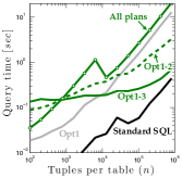
(a) $4$-chain queries

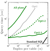
(b) $7$-chain queries

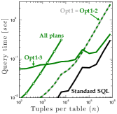
(c) $2$-star queries

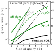
(d) $k$-chain queries

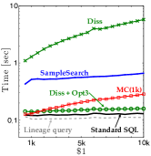
(e) $2 = %red%green%

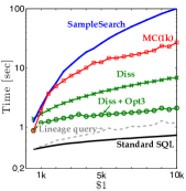
(f) $2 = %red%

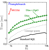
(g) $2 = %

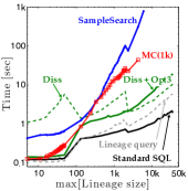
(h) Combining (a)-(c)

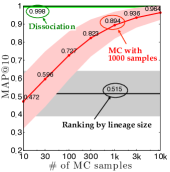
(i) Section 5.2

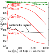
(j) Section 5.2

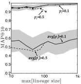
(k) Section 5.2

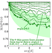
(l) Section 5.2

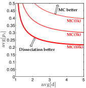
(m) Section 5.2

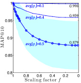
(n) Section 5.2

(o) Section 5.2

(p) Section 5.2

Figure 5: Timing results: (a)-(c) For increasing database sizes and constant cardinalities, our optimizations approach deterministic SQL performance. (d) Our optimizations can even evaluate very large number of minimal plans efficiently (here shown up to 429 for an 8-chain query). (e)-(h) For the TPC-H query, the best evaluation for dissociation is within a factor of $6$ of that for deterministic query evaluation. (i)-(p) Ranking experiments on TPC-H: Assumptions for each subfigure and conclusions that can be drawn are described in the main text in the respective result paragraph.

Question 5.24.

How does dissociation compare against other probabilistic methods and standard query evaluation?

Result 2. The best evaluation strategy for dissociation takes only a small overhead over standard SQL evaluation and is considerably faster than other probabilistic methods for large lineages.

Figures 5d to 5h show that SampleSearch does not scale to larger lineages as the performance of exact probabilistic inference depends on the tree-width of the Boolean lineage formula, which generally increases with the size of the data. In contrast, dissociation is independent of the treewidth. For example, SampleSearch needed 780 sec for calculating the ground truth for a query with $\max[\textrm{lin}]=5.9$k for which dissociation took 3.0 sec, and MC(1k) took 42 sec for a query with $\max[\textrm{lin}]=4.2$k for which dissociation took 2.4 sec. Dissociation takes only 10.5 sec for our largest query $\$2=\textup{{\small'\%'}}$ and $\$1=10k$ with $\max[\textrm{lin}]=35$k. Retrieving the lineage for that query alone takes 5.8 sec, which implies that any probabilistic method that evaluates the probabilities outside of the database engine needs to issue this query to retrieve the DNF for each answer and would thus have to evaluate lineages of sizes around 35k in only 4.7 (= 10.5 - 5.8) sec to be faster than dissociation.

5.2 Ranking experiments

For the following experiments, we are limited to those query parameters $1 and $2 for which we can get the ground truth (and results from MC) in acceptable time. We systematically vary $p_{i\max}$ between $0.1$ and $1$ (and thus $\textrm{avg}[p_{i}]$ between $0.05$ and $0.5$) and evaluate the rankings several times over randomly assigned input tuple probabilities. We only keep data points (i.e. results of individual ranking experiments) for which the output probabilities are not too close to 1 to be meaningful ($\max[p_{a}]<0.999\,999$).

Question 5.25.

How does ranking quality compare for our three ranking methods and which are the most important factors that determine the quality for each method?

Result 3. Dissociation performs better than MC which performs better than ranking by lineage size.

Fig.​ 5i shows averaged results of our probabilistic methods for $\$2=\textup{{\small'\%red\%green\%'}}$. Shaded areas indicate standard deviations and the x-axis shows varying numbers of MC samples. We only used those data points for which $\textrm{avg}[p_{a}]$ of the top 10 ranked tuples is between $0.1$ and $0.9$ according to ground truth ($\approx 6$k data points for dissociation and lineage, $\approx 60$k data points for MC, as we repeated each MC simulation 10 times), as this is the best regime for MC, according to Section 5.2. We also evaluated quality for dissociation and ranking by lineage for more queries by choosing parameter values for $\$2$ from a set of 28 strings, such as ’%r%g%r%a%n%d%’ and ’%re%re%’. The average MAP over all 28 choices for parameters $2 is 0.997 for ranking by dissociation and 0.520 for ranking by lineage size ($\approx 100$k data points). Most of those queries have too large of a lineage to evaluate MC. Note that ranking by lineage always returns the same ranking for given parameters $1 and $2, but the GT ranking would change with different input probabilities.

Result 4. Ranking quality of MC increases with the number of samples and decreases when the average probability of the answer tuples $\textrm{avg}[p_{a}]$ is close to $0$ or $1$.

Fig.​ 5j shows the AP as a function of $\textrm{avg}[p_{a}]$ of the top 10 ranked tuples according to ground truth by logarithmic scaling of the x-axis (each point in the plot averages AP over $\approx 450$ experiments for dissociation and lineage and over $\approx 4.5$k experiments for MC). We see that MC performs increasingly poor for ranking answer tuples with probabilities close to $0$ or $1$ and even approach the quality of random ranking (MAP@10 = 0.22). This is so because, for these parameters, the probabilities of the top 10 answers are very close, and MC needs many iterations to distinguish them. Therefore, MC performs increasingly poorly for increasing size of lineage but fixed average input probability $\textrm{avg}[p_{i}]\approx 0.5$, as the average answer probabilities $\textrm{avg}[p_{a}]$ will be close to $1$. In order not to “bias against our competitor,” we compared against MC in its best regime with $0.1<\textrm{avg}[p_{a}]<0.9$ in Fig.​ 5i.

Result 5. Ranking by lineage size has good quality only when all input tuples have the same probability.

Fig.​ 5k shows that ranking by lineage is good only when all tuples in the database have the same probability (labeled by $p_{i}=\textrm{const}$ as compared to $\textrm{avg}[p_{i}]=\textrm{const}$). This is a consequence of the output probabilities depending mostly on the size of the lineages if all probabilities are equal. Dependence on other parameters, such as overall lineage size and magnitude of input probabilities (here shown for $p_{i}=0.1$ and $p_{i}=0.5$), seem to matter only slightly.

Result 6. The quality of dissociation decreases with the average number of dissociations per tuple $\textrm{avg}[d]$ and with the average input probabilities $\textrm{avg}[p_{i}]$. Dissociation performs very well and notably better then MC(10k) if either $\textrm{avg}[d]$ or $\textrm{avg}[p_{i}]$ are small.

Each answer tuple $a$ gets its score $p_{a}$ from one of two query plans $P_{S}$ and $P_{P}$ that dissociate tuples in tables $S$ and $P$, respectively. For example, if the lineage size for tuple $a$ is 100 and the lineage contains 20 unique suppliers from table $S$ and 50 unique parts from table $P$, then $P_{S}$ dissociates each tuple from $S$ into 5 tuples and $P_{P}$ each tuple from $P$ into $2$ tuples, on average. Most often, $P_{P}$ will then give the better bounds as it has fewer average dissociations. Let $\textrm{avg}[d]$ be the mean number of dissociations for each tuple in the dissociated table of its respective optimal query plan, averaged across all top 10 ranked answer tuples. For all our queries (even those with $\$1=10k$ and $\$2=\textup{{\small'\%'}}$), $\textrm{avg}[d]$ stays below $1.1$ as, for each tuple, there is usually one plan that dissociates few variables. In order to understand the impact of higher numbers of dissociations (increasing $\textrm{avg}[d]$), we also measured AP for the ranking for each query plan individually. Hence, for each choice of random parameters, we record two new data points – one for ranking all answer tuples by using only $P_{S}$ and one for using only $P_{P}$ – together with the values of $\textrm{avg}[d]$ in the respective table that gets dissociated. This allows us to draw conclusions for a larger set of parameters. Fig.​ 5l plots MAP values as a function of $\textrm{avg}[d]$ of the top 10 ranked tuples on the horizontal axis, and various values of $\textrm{avg}[p_{i}]$ ($\textrm{avg}[p_{i}]=0.05,0.10,\ldots,0.5$). Each plotted point averages over at least 10 data points (some have 10, other several 1000s). Dashed lines show a fitted parameterized curve to the data points on $\textrm{avg}[p_{i}]$ and $\textrm{avg}[d]$. The figure also shows the standard deviations as shaded areas for $\textrm{avg}[p_{i}]=0.5$. We see that the quality is very dependent on $\textrm{avg}[p_{i}]$, as predicted by Prop. 3.13.

Fig.​ 5m maps the trade-off between dissociation and MC for the two important parameters for the quality of dissociation ($\textrm{avg}[d]$ and $\textrm{avg}[p_{i}]$) and the number of samples for MC. For example, MC(1k) gives a better expected ranking than dissociation only for the small area above the thick red curve marked MC(1k). For MC, we used the test results from Fig.​ 5i; i.e. assuming $0.1<\textrm{avg}[p_{a}]<0.9$ for MC. Also recall that for large lineages, having an input probability with $\textrm{avg}[p_{i}]=0.5$ will often lead to answer probabilities close to $1$ for which ranking is not possible anymore (recall Fig.​ 5k). Thus, for large lineages, we need small input probabilities to have meaningful interpretations. And for small input probabilities, dissociation considerably outperforms any other method.

Question 5.26.

How much would the ranking change according to exact probabilistic inference if we scale down all input tuples?

Result 7. If the probabilities of all input tuples are already small, then scaling them further down does not affect the ranking much.

Here, we repeatedly evaluated the exact ranking for 7 different parameterized queries over randomly generated databases with one query plan that has $\textrm{avg}[d]\approx 3$, for two conditions: first on a probabilistic database with $avg[p_{i}]$ input probabilities (we defined the resulting ranking as GT); then again on a scaled version, where all input probabilities in the database are multiplied by the same scaling factor $f\in(0,1)$. We then compared the new ranking against GT. Fig.​ 5n shows that if all input probabilities are already small (and dissociation already works well), then scaling has little effect on the ranking. However, for $avg[p_{i}]=0.5$ (and thus many tuples with $p_{i}$ close to $1$), we have a few tuples with $p_{i}$ close to $1$. These tuples are very influential for the final ranking, but their relative influence decreases if scaled down even slightly. Also note that even for $avg[p_{i}]=0.5$, scaling a database by a factor $f=0.01$ instead of $f=0.2$ does not make a big difference. However, the quality remains well above ranking by lineage size (!). This suggests that the difference between ranking by lineage size (MAP $\approx 0.529$) and the ranking on a scaled database for $f\rightarrow 0$ (MAP $\approx 0.879$) can be attributed to the relative weights of the input tuples (we thus refer to this as “ranking by relative input weights”). The remaining difference in quality then comes from the actual probabilities assigned to each tuple. Using MAP $\approx 0.220$ as baseline for random ranking, 38% of the ranking quality can be found by the lineage size alone vs. 85% by the lineage size plus the relative weights of input tuples. The remaining 15% come from the actual probabilities (Fig.​ 5o).

Question 5.27.

Does the expected ranking quality of dissociation decrease to random ranking for increasing fractions of dissociation (just like MC does for decreasing number of samples)?

Result 8. The expected performance of dissociation for increasing $\textrm{avg}[d]$ for a particular query is lower bounded by the quality of ranking by relative input weights.

Here, we use a similar setup as before and now compare various rankings against each other: SampleSearch on the original database (“GT”); SampleSearch on the scaled database (“Scaled GT”); dissociation on the scaled database (“Scaled Diss”); and ranking by lineage size (which is unaffected by scaling). From Fig.​ 5p, we see that the quality of Scaled Diss w.r.t. Scaled GT $\rightarrow 1$ for $f\rightarrow 0$ since dissociation works increasingly well for small $\textrm{avg}[p_{i}]$ (recall Prop. 3.13). We also see that Scaled Diss w.r.t. GT decreases towards Scaled GT w.r.t. GT for $f\rightarrow 0$. Since dissociation can always reproduce the ranking quality of ranking by relative input weights by first downscaling the database (though losing information about the actual probabilities) the expected quality of dissociation for smaller scales does not decrease to random ranking, but rather to ranking by relative weights. Note this result only holds for the expected MAP; any particular ranking can still be very much off.

6 Related Work

Probabilistic databases. Current approaches to query evaluation on probabilistic databases can be classified into three categories: ($i$) incomplete approaches identify tractable cases either at the query-level [7, 8, 17] or the data-level [38, 46, 50]; ($ii$) exact approaches [2, 30, 38, 39, 49] work well on queries with simple lineage expressions, but perform poorly on database instances with complex lineage expressions. ($iii$) approximate approaches either apply general purpose sampling methods [29, 32, 33, 44], or approximate the number of models of the Boolean lineage expression [16, 40, 45]. Our work can be seen as a generalization of several of these techniques: Our algorithm returns the exact score if the query is safe [7, 39] or data-safe [30].

Lifted and approximate inference. Lifted inference was introduced in the AI literature as an approach to probabilistic inference that uses the first-order formula to exploit symmetries at the grounded level [42]. This research evolved independently of that on probabilistic databases, and the two have many analogies: A formula is called domain liftable iff its data complexity is in polynomial time [28], which is the same as a safe query in probabilistic databases, and the FO-d-DNNF circuits described in [12] correspond to the safe plans discussed in this paper. See [11] for a recent discussion on the similarities and differences.

Representing Correlations. The most popular approach to represent correlations between tuples in a probabilistic database is by a Markov Logic network (MLN) which is a set of soft constraints [13]. Quite remarkably, all complex correlations introduced by an MLN can be rewritten into a query over a tuple-independent probabilistic database [24, 26, 31]. In combination with such rewritings, our techniques can be also applied to MLNs if their rewritings results in conjunctive queries without self-joins.

Dissociation. Dissociation was first introduced in the workshop paper [20], presented as a way to generalize graph propagation algorithms to hypergraphs. Theoretical upper and lower bounds for dissociation of Boolean formulas, including Theorem 2, were proven in [22]. Dissociation is related to a technique called relaxation for probabilistic inference in graphical models [10].

7 Conclusions and Outlook

This paper proposes to approximate probabilistic query evaluation by evaluating a fixed number of query plans, each providing an upper bound on the true probability, then taking their minimum. We provide an algorithm that takes into account important schema information to enumerate only the minimal necessary plans among all possible plans, and prove it to be a strict generalization of all known results of PTIME self-join-free conjunctive queries. We describe relational query optimization techniques that allow us to evaluate all minimal queries in a single query and very fast: Our experiments show that these optimizations bring approximate probabilistic query evaluation close to standard query evaluation while providing high ranking quality. In future work, we plan to generalize this approach to full first-order queries. We will also make slides illustrating our algorithms available at http://LaPushDB.com.

Acknowledgements. This work was supported in part by NSF grants IIS-0513877, IIS-0713576, IIS-0915054, and IIS-1115188. We thank the reviewers for their careful reading of this manuscript and their detailed feedback. WG would also like to thank Manfred Hauswirth for a small comment in 2007 that was crucial for the development of the ideas in this paper.

References

- [1] A. Amarilli, Y. Amsterdamer, and T. Milo. Uncertainty in crowd data sourcing under structural constraints. In DASFAA Workshops, pp. 351–359, 2014.
- [2] L. Antova, T. Jansen, C. Koch, and D. Olteanu. Fast and simple relational processing of uncertain data. In ICDE, pp. 983–992, 2008.
- [3] L. Antova, C. Koch, and D. Olteanu. Maybms: Managing incomplete information with probabilistic world-set decompositions. In ICDE, pp. 1479–1480, 2007.
- [4] P. Beame, J. Li, S. Roy, and D. Suciu. Model counting of query expressions: Limitations of propositional methods. In ICDT, pp. 177–188, 2014.
- [5] A. Carlson, J. Betteridge, B. Kisiel, B. Settles, E. R. H. Jr., and T. M. Mitchell. Toward an architecture for never-ending language learning. In AAAI, 2010.
- [6] Y. Chen and D. Z. Wang. Knowledge expansion over probabilistic knowledge bases. In SIGMOD, pp. 649–660, 2014.
- [7] N. N. Dalvi and D. Suciu. Efficient query evaluation on probabilistic databases. VLDB J., 16(4):523–544, 2007.
- [8] N. N. Dalvi and D. Suciu. The dichotomy of probabilistic inference for unions of conjunctive queries. J. ACM, 59(6):30, 2012.
- [9] DeepDive: http://deepdive.stanford.edu/.
- [10] G. V. den Broeck, A. Choi, and A. Darwiche. Lifted relax, compensate and then recover: From approximate to exact lifted probabilistic inference. In UAI, pp. 131–141, 2012.
- [11] G. V. den Broeck and D. Suciu. Lifted probabilistic inference in relational models. In UAI tutorials, 2014.
- [12] G. V. den Broeck, N. Taghipour, W. Meert, J. Davis, and L. D. Raedt. Lifted probabilistic inference by first-order knowledge compilation. In IJCAI, pp. 2178–2185, 2011.
- [13] P. Domingos and D. Lowd. Markov Logic: An Interface Layer for Artificial Intelligence. Morgan & Claypool Publishers, 2009.
- [14] X. Dong, E. Gabrilovich, G. Heitz, W. Horn, N. Lao, K. Murphy, T. Strohmann, S. Sun, and W. Zhang. Knowledge vault: A web-scale approach to probabilistic knowledge fusion. In KDD, pp. 601–610, 2014.
- [15] B. Ermis and G. Bouchard. Scalable binary tensor factorization. In UAI, 2014.
- [16] R. Fink and D. Olteanu. On the optimal approximation of queries using tractable propositional languages. In ICDT, pp. 174–185, 2011.
- [17] R. Fink and D. Olteanu. A dichotomy for non-repeating queries with negation in probabilistic databases. In PODS, pp. 144–155, 2014.
- [18] N. Fuhr and T. Rölleke. A probabilistic relational algebra for the integration of information retrieval and database systems. ACM Trans. Inf. Syst., 15(1):32–66, 1997.
- [19] W. Gatterbauer, S. Günnemann, D. Koutra, and C. Faloutsos. Linearized and single-pass belief propagation. PVLDB, 8(5), 2015. (CoRR abs/1406.7288).
- [20] W. Gatterbauer, A. K. Jha, and D. Suciu. Dissociation and propagation for efficient query evaluation over probabilistic databases. In MUD, pp. 83–97, 2010.
- [21] W. Gatterbauer and D. Suciu. Dissociation and propagation for efficient query evaluation over probabilistic databases. CoRR abs/1310.6257, 2013.
- [22] W. Gatterbauer and D. Suciu. Oblivious bounds on the probability of Boolean functions. ACM Trans. Database Syst., 39(1):5, 2014. (CoRR abs/1409.6052).
- [23] V. Gogate and P. Domingos. Formula-based probabilistic inference. In UAI, pp. 210–219, 2010.
- [24] V. Gogate and P. Domingos. Probabilistic theorem proving. In UAI, pp. 256–265, 2011.
- [25] C. P. Gomes, A. Sabharwal, and B. Selman. Model counting. In Handbook of Satisfiability, pp. 633–654. 2009.
- [26] A. D. Guy Van den Broeck, Wannes Meert. Skolemization for weighted first-order model counting. In KR, 2014.
- [27] J. Hoffart, F. M. Suchanek, K. Berberich, and G. Weikum. Yago2: A spatially and temporally enhanced knowledge base from wikipedia. Artif. Intell., 194:28–61, 2013.
- [28] M. Jaeger and G. V. den Broeck. Liftability of probabilistic inference: Upper and lower bounds. In StaRAI, 2012.
- [29] R. Jampani, F. Xu, M. Wu, L. L. Perez, C. M. Jermaine, and P. J. Haas. MCDB: a Monte Carlo approach to managing uncertain data. In SIGMOD, pp. 687–700, 2008.
- [30] A. Jha, D. Olteanu, and D. Suciu. Bridging the gap between intensional and extensional query evaluation in probabilistic databases. In EDBT, pp. 323–334, 2010.
- [31] A. K. Jha and D. Suciu. Probabilistic databases with markoviews. PVLDB, 5(11):1160–1171, 2012.
- [32] S. Joshi and C. M. Jermaine. Sampling-based estimators for subset-based queries. VLDB J., 18(1):181–202, 2009.
- [33] O. Kennedy and C. Koch. PIP: A database system for great and small expectations. In ICDE, pp. 157–168, 2010.
- [34] C. D. Manning, P. Raghavan, and H. Schütze. Introduction to Information Retrieval. Cambridge University Press, 2008.
- [35] F. McSherry and M. Najork. Computing information retrieval performance measures efficiently in the presence of tied scores. In ECIR, pp. 414–421, 2008.
- [36] F. Niu, C. Ré, A. Doan, and J. W. Shavlik. Tuffy: Scaling up statistical inference in markov logic networks using an RDBMS. PVLDB, 4(6):373–384, 2011.
- [37] OEIS: The on-line encyclopedia of integer sequences: http://oeis.org/.
- [38] D. Olteanu and J. Huang. Using OBDDs for efficient query evaluation on probabilistic databases. In SUM, pp. 326–340, 2008.
- [39] D. Olteanu, J. Huang, and C. Koch. Sprout: Lazy vs. eager query plans for tuple-independent probabilistic databases. In ICDE, pp. 640–651, 2009.
- [40] D. Olteanu, J. Huang, and C. Koch. Approximate confidence computation in probabilistic databases. In ICDE, pp. 145–156, 2010.
- [41] J. Pearl. Probabilistic reasoning in intelligent systems: networks of plausible inference. Morgan Kaufmann Publishers, 1988.
- [42] D. Poole. First-order probabilistic inference. In IJCAI, pp. 985–991, 2003.
- [43] PostgreSQL 9.2: http://www.postgresql.org/download/.
- [44] C. Ré, N. N. Dalvi, and D. Suciu. Efficient top-k query evaluation on probabilistic data. In ICDE, pp. 886–895, 2007.
- [45] C. Ré and D. Suciu. Approximate lineage for probabilistic databases. PVLDB, 1(1):797–808, 2008.
- [46] S. Roy, V. Perduca, and V. Tannen. Faster query answering in probabilistic databases using read-once functions. In ICDT, pp. 232–243, 2011.
- [47] SampleSearch: http://www.hlt.utdallas.edu/~vgogate/SampleSearch.html.
- [48] P. G. Selinger, M. M. Astrahan, D. D. Chamberlin, R. A. Lorie, and T. G. Price. Access path selection in a relational database management system. In SIGMOD, pp. 23–34, 1979.
- [49] P. Sen and A. Deshpande. Representing and querying correlated tuples in probabilistic databases. In ICDE, pp. 596–605, 2007.
- [50] P. Sen, A. Deshpande, and L. Getoor. Read-once functions and query evaluation in probabilistic databases. PVLDB, 3(1):1068–1079, 2010.
- [51] A. P. Singh and G. J. Gordon. Relational learning via collective matrix factorization. In KDD, pp. 650–658, 2008.
- [52] J. Stoyanovich, S. B. Davidson, T. Milo, and V. Tannen. Deriving probabilistic databases with inference ensembles. In ICDE, pp. 303–314, 2011.
- [53] D. Suciu, D. Olteanu, C. Ré, and C. Koch. Probabilistic Databases. Morgan & Claypool Publishers, 2011.
- [54] TPC-H benchmark: http://www.tpc.org/tpch/.
- [55] K. Zeng, S. Gao, B. Mozafari, and C. Zaniolo. The analytical bootstrap: a new method for fast error estimation in approximate query processing. In SIGMOD, pp. 277–288, 2014.
- [56] C. Zhang and C. Ré. Towards high-throughput Gibbs sampling at scale: a study across storage managers. In SIGMOD, pp. 397–408, 2013.