Complete list of the ASTRO-H Science Working Group

Abstract

This white paper addresses selected new (to X-ray astronomy) physics and data analysis issues that will impact ASTRO-H SWG observations as a result of its high-spectral-resolution X-ray microcalorimeter, the focussing hard X-ray optics and corresponding detectors, and the low background soft $\gamma$-ray detector. We concentrate on issues of atomic and nuclear physics, including basic bound-bound and bound-free transitions as well as scattering and radiative transfer. The major topic categories include the physics of charge exchange, solar system X-ray sources, advanced spectral model, radiative transfer, and hard X-ray emission lines and sources.

1 Introduction

This white paper describes a number of new spectral features, arising from previously hard-to-observe processes, that will be detectable with ASTRO-H, primarily with the SXS detector but also using the hard X-ray and soft gamma ray detectors. In particular, charge exchange (CX) between atoms and ions will create diagnostic soft X-ray emission lines that should be visible from a number of astrophysical environments, including solar wind interactions with planets, comets, and even the heliosphere. In addition to CX with the solar wind CX, this may also occur in more distant regions such as supernova remnants and starburst galaxies, although this remains speculative. Deep ASTRO-H observations with the SXS with non-dispersive high-resolution spectroscopy should reveal if CX is in fact occurring.

2 The Physics of Charge Exchange

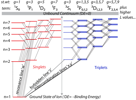
Figure 1: Schematic Grotrian diagram for a Helium-like ion with selected radiative (downward) transitions marked as dashed lines. Charge exchange transitions between a hydrogenic ion and a neutral hydrogen atom with binding energy -13.6 eV will result in an ionized hydrogen ion and a highly excited Helium-like state; for O VII this is $n\approx 6$.

The charge exchange (CX) process simply transfers an electron from one atom or ion to another. Although there can be a change in momentum, no photon is created via the electron transfer itself. Instead the electron maintains roughly the same binding energy in the process of moving from one atom to another, so the recipient ion is usually left in a highly-excited state that then radiatively stabilizes. Typically, astrophysical charge exchange involves a donor hydrogen atom and a highly ionized metal recipient such as O⁺⁷ or Si⁺¹⁰, although in some cases such as comets (Cravens, 2002) or planets in the Solar system (Bhardwaj, 2007) the donors can be metals or molecules. Evaluating the impact of this process on X-ray spectra involves some fundamental difficulties, both in the atomic physics and the astrophysics.

2.1 Atomic Process

From an atomic physics perspective, the exact cross section for charge exchange into a particular quantum state at low to moderate impact energies (relative to the binding energies) is difficult to calculate theoretically, although a number of results are now available for selected ions (e.g. Kharchenko & Dalgarno, 2001; Kharchenko et al., 2003). Cross sections at larger energies are much easier to determine, and are in fact readily available from the fusion community (see, for example, http://www.adas-fusion.eu/theme.php?id=2). CX provides an efficient means of heating tokamak plasmas since the fast-moving neutral atoms easily pass through the magnetic confinement and transfer their energy to the plasma.

At low energies, the simplest possible approximate cross section for CX is simply a constant, $\sigma_{\rm CX}\sim 3\times 10^{-15}$ cm^-2, which is normally accurate to about a factor of 3. For a somewhat more accurate approximation one can follow Wegmann et al. (1998), who use a hydrogenic model for the CX cross section into the highly-excited state:

$$\sigma_{\rm CX}=8.8\times 10^{-17}{\rm cm}^{2}\ {{q-1}\over{{{q^{2}}\over{2n^{2}}}-|I_{p}|}}$$ (1)

where $q$ is the charge of the ion, $I_{p}$ is the ionization potential in atomic units (i.e., 1 au = 27.2 eV) of the target ‘donor’ atom, and $n$ the principal quantum number. Since the total cross section must be positive, $n$ has a maximum value depending upon the charge of the ion. For O⁺⁸ interacting with neutral H, therefore, $q=8$, $I_{p}=0.5$, and $n<8$. With $n=7$, the approximate cross section is $4\times 10^{-15}$ cm^-2, while for $n=6$ it is $1.6\times 10^{-15}$ cm^-2. Once the electron has been ‘exchanged’ onto a highly-excited level of the ion, “charge exchange” photons resulting from radiative decays of the highly-exited ion are created (see Figure 1). Effectively, the electron decays towards the ground state like a pachinko ball, radiating photons at each step. As implied by Figure 1, this means that CX into a He-like triplet state will lead to enhanced forbidden and intercombination lines (as almost any exchange into a triplet state results in such lines). It is worth noting that these lines can be created via normal collisional and photoionization processes as well; CX merely increases the rate of highly-excited transitions. Thus CX into the He-like singlet state will lead to enhanced (relative to a purely collisional model in the ground state) high-$n$ resonance transitions from $np{}^{1}P_{1}$ to the ground state. The atomic structure and radiative transition data can be used to determine the spectrum emitted as the ion stabilizes by radiative decay. In cases where the initial electron transfer would put the ion in a higher state than is available in AtomDB v2.0.2, which typically extends to $n=5$ at a minimum and to $n=10$ for the hydrogenic and helium-like isosequences, a new set of calculations (up to $n=14$) have been complete to enable the necessary spectral calculations. Figure 2 shows a series of comparisons of one common diagnostic, the He-like G ratio, for CX and other plasmas.

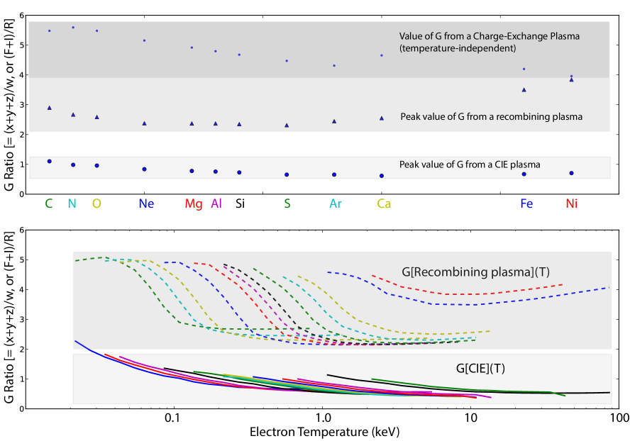
Figure 2: [Top] The peak of the G-ratio from helium-like ions, defined as the ratio of the forbidden and intercombination lines to the resonance line, for each abundant element in three different common plasma situations: a CIE plasma, a recombining plasma, and a charge-exchange-dominated plasma. [Bottom] The G ratio as a function of electron temperature in the CIE and recombining cases. Note that CX is not shown as it is temperature-independent.

A key residual uncertainty in low-energy CX cross sections is the angular momentum of the exchanged electron, which will impact the decay path and thus the emitted photons (e.g. in Figure 1, the singlet versus triplet state). The simplest possible approximation would be to simply distribute states evenly by the total angular momentum, or to distribute them by the statistical weight of each level. Janev & Winter (1985) outlined more sophisticated theoretical models for state selective charge exchange (SSCX) models, depending on the relative velocity of the ions $v$ and the characteristic orbital velocity $v_{\mathrm{o}}=\sqrt{2I/m_{e}}$, where I is the ionization potential of the initial level of the donor electron (e.g. 13.6 eV for ground state H), and $m_{e}$ is the electron mass. For the case of the solar wind ($v\approx 400$ km s^-1) and a hydrogenic donor, the low velocity regime ($v/v_{\mathrm{o}}<1$) applies. They considered two different distributions:

1. “Landau-Zener:”, weighted by the function

   $$W(l)={{l(l+1)(2l+1)\times(n-1)!\times(n-2)!}\over{(n+l)!\times(n-l-1)!}}$$ (2)

2. “Separable:” weighted by the function

   $$W(l)={{(2l+1)}\over{Z}}\times\exp\Big{[}{{-l\times(l+1)}\over{z}}\Big{]}$$ (3)

These two different distributions do not lead to large changes in the resulting spectrum, so both should be considered as possibilities that partially address the range of uncertainties in this approach.

2.2 Astrophysical Modeling

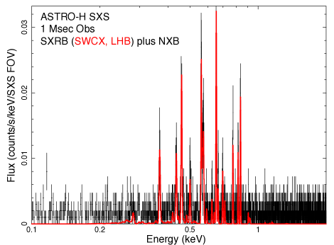
Figure 3: Soft X-ray background model, simulated using simx, assuming a combined LHB and SWCX model that fits the DXS spectrum and CHIPS upper limits (Smith et al. 2014).

A more significant problem exists in the astrophysical modeling, as it is not possible to determine with any accuracy the density of donor atoms and recipient ions in a given region of space. Individual situations do exist where these can be estimated, such as charge exchange in the solar wind where ions in the solar wind are directly measured by satellites like ACE and WIND and models exist for the geocoronal or heliospheric neutral atoms (Koutroumpa et al., 2006, 2009). Thus, while there remain many ions without explicit cross section calculations, these are matched by our lack of knowledge of the mixing in hot plasma / dense cloud interaction regions that could lead to CX spectra. Although not ideal, these difficulties mean that any approximations in the model will not dominate the inherent uncertainties in the final result.

The CX rate along a line of sight during an astrophysical observation can be written as $F_{CX}=(4\pi D^{2})^{-1}\int{n_{D}n_{R}v\sigma^{cx}_{D\rightarrow R}(E)dV}$ where $N_{CX}$ is the number of CX reactions in the volume, $n_{D}$ and $n_{R}$ are the donor and recombining ion densities, and $\sigma^{cx}_{D\rightarrow R}(E)$ is the energy-dependent cross section for charge exchange between the donor and recombining ions at velocity $v$. In the case of solar wind charge exchange (SWCX), the donor ions will be neutral hydrogen or helium atoms in the interstellar medium, while the recombining ions will be the solar wind ions. Of the parameters determining the CX rate, both $n_{R}$ and $n_{D}$, and their variation within the volume are unknown, and $v$ can only be roughly estimated. In the interest of developing an approximate model, fine accuracy for the total charge exchange cross section can be set aside in order to obtain relative partial capture cross sections into different $n$ and $l$ shells, as described above. This can be used to predict the shape of the CX spectrum, although absolute magnitudes will have to be obtained from fits to spectra and discretion during analysis.

The actual line strengths in this approximation can be determined using the atomic structure and radiative transition data available in the AtomDB v2.0.2 (http://www.atomdb.org). If the initial electron transfer would put the ion in a higher state than is available in the AtomDB (which typically extends to $n=5$ at a minimum for ions that can emit X-rays in a collisional plasma and to $n=10$ for the hydrogenic and helium-like isosequences), then more atomic data are needed. For these ions Smith et al. (2012); Foster et al. (2014) performed a large atomic structure calculation to determine the energies and radiative transition rates of all levels up to at least $n^{\prime}$, the predicted state of the post-CX system. We calculated all ions of astrophysical interest up to $n\leq 13$ (in Ni⁺²⁷) using the Autostructure (Badnell, 1986) code. The largest number of levels needed (for the ion Ni⁺²⁰) was 2,374. Until fairly recently, these calculations were simply not feasible given computational limitations, but now the primary limitation is the time required to set up the calculations and to check the results.

A first cut of this spectral model that can be used within XSPEC (or ISIS) is available at http://www.atomdb.org/acx. Smith et al. (2014) used this model to fit the Diffuse X-ray Spectrometer (DXS) data as well as the Cosmic Hot Interstellar Plasma Spectrometer (CHIPS) using a model that combines a hot thermal plasma (representing the Local Hot Bubble) plus a two component SWCX model (representing the Fast and Slow solar winds). While there are strong indications that the SWCX components are time-variable, this should give a reasonable idea of what level of line emission could be expected. A simulated 1 Msec spectrum is shown in Figure 3 for the SXS, including the non-X-ray-background (NXB) as well.

3 Charge Exchange in the Solar System and Beyond

In recent years, many sources of soft X-rays within the solar system, besides the Sun itself, have been discovered. This has opened the door to new studies of the mechanisms and the physics responsible for the emission.

In particular, in Solar Wind Charge eXchange (SWCX), highly ionized ions in the solar wind collide with neutral atoms picking up an electron in an excited state. The electron then decays producing UV and X-ray emission. SWCX was originally discovered from observations of comets, where solar wind would “charge exchange” with the neutrals in the comet (Cravens et al., 1997). It is now believed that solar wind also “charge exchanges” with neutrals in our atmosphere (magnetosheath SWCX) (Cravens 2001, Robertson and Cravens 2003a,b) and with interstellar neutrals in the solar system (heliospheric SWCX) (Cox, 1998).

Many solar system planets have also been recognized to show X-ray emission. The detected objects are Mercury, Venus, Earth, Mars, Jupiter, and Saturn (see Bhardwaj et al. 2007; Ezoe et al. 2011a, 2012 for review).

Preliminary studies with current and past missions have been quite fruitful in laying the groundwork for the understanding of the X-ray emission and the mechanisms behind them. However, this studies are still in their infancy and many of the fundamental physical parameters are still unknown. In particular, current missions lack the energy resolution necessary to resolve the many emission lines associated with these processes and any significant response in the $1/4$ keV energy band, where a significant fraction of the emission lies. The time required for each observation and the time variation of the emission has also limited the number of observations available.

The high energy resolution of the ASTRO-H SXS instrument should bring significant improvements in at least two if these areas.

3.1 Introduction

Fully characterizing and modeling the SWCX emission requires an understanding of the distribution of neutral material in the magnetosheath and heliosphere, the properties and distribution of the solar wind, and the interaction cross-sections. SWCX emission probes both the solar wind and the distribution of neutral atoms throughout the solar system, complementing many other heliophysical measurements.

However, understanding SWCX emission is also critical to astrophysical observations, as it contributes a significant background to X-ray observations of extended objects that may be inseparable from the signal of interest, as many of the emission lines are the same used as plasma diagnostics of thermal emission. It is, in particular, essential to understanding the nature and structure of the Local Hot Bubble (LHB) surrounding the Sun. Finally, soft X-ray studies of planets also offer a new tool for remotely studying their atmosphere and environment.

Solar Wind Charge eXchange

Four components of SWCX can be identified and characterized using ASTRO-H:

1. Heliospheric

2. Geocoronal

3. Cometary

4. Planetary

The first two components directly affect the emission from the Diffuse X-ray Background (DXB) and other extended object emission. The last two can be used directly to probe the physics and composition of the objects themselves. Cometary SWCX can also be used to study the properties of “fast” solar wind, which is emitted at high ecliptic latitude. SWCX is the only component of the DXB with a “short scale” temporal variation due to the flux of ions in the solar wind that can be used to identify it on top of the other components.

Geocoronal, planetary, and cometary SWCX are varying on a very short time scale of hours to days, due to the interaction of solar wind with neutral concentrated in a small volume (a planet’s atmosphere or a comet surface), while heliospheric SWCX varies more smoothly on a time scale of several days to months, due to the diffusion time of the wind through the solar system. An annual modulation due to distributions of interstellar neutrals (H and He) passing through the solar system is also present.

Above 0.3 keV SWCX emission consists mostly of K-shell lines of C, N, O, Ne, and Mg, and L-shell lines of Fe. To first order, the line intensity depends linearly on solar wind conditions. In particular, the intensity $I$ is the integral over the line of sight $ds$ of the product of the ion density $n_{ION}$, the neutral density ($n_{H}$ and $n_{H}e$), and the interaction cross-section

$$I_{OVII}=\int\alpha_{ION}n_{ION}(n_{H}+n_{He})\langle g\rangle ds,$$ (4)

where $\langle g\rangle$ is average solar wind speed, and the cross-sections $\alpha_{ION}$ are velocity dependent.

Solar wind data are available through the ACE, WIND, and STEREO-A/B missions. The combination of SWEPAM and SWICS instruments aboard ACE provide $\langle g\rangle$ and $n_{ION}$ (at least for oxygen), while an ASTRO-H campaign will be essential to measure the cross sections $\alpha_{ION}$ for different solar wind conditions (as they are velocity dependent), the distribution of neutrals $n_{H}$ and $n_{He}$ as a function of pointing direction, and the ratio n_OVIII/n_OVII as a function of solar wind conditions. In addition to the invaluable contribution to the physics of SWCX, such parameters are paramount for the future prediction and evaluation of SWCX contribution to astrophysical observations with existing (XMM-Newton, Chandra, Suzaku) observations and future missions (eROSITA, AXSIO, Athena).

Directly evaluating the effect of background due to SWCX on observations of diffuse object with current and future missions is, in general, impossible, and modeling its effect remains, in many cases, the only long-term viable option. While there are well-defined models for SWCX emission from the heliosphere, testing them is problematic. Koutroumpa et al. (2007), using a self consistent model of the heliospheric SWCX emission, managed to associate observed discrepancies in XMM-Newton and Suzaku observations separated by several years with solar cycle-scale variations of the heliospheric SWCX emission. A more recent paper (Snowden 2009) was successful in using an XMM-Newton observation to test a model (Robertson & Cravens 2003a) for emission from the near-Earth environment.

Koutroumpa et al. (2009) uses a different series of XMM-Newton observations to search for SWCX emission from the He focusing cone. They were relatively successful, but the detection was at a marginal level due to the short exposures and higher backgrounds experienced by XMM-Newton. A critical aspect of all future investigations of extended objects will be to test and upgrade our current SWCX models, specifically where it pertains the input parameters discussed above.

SWCX, Local Hot Bubble, and extended sources

It has been suggested that SWCX emission may actually be responsible for all of the “local flux” observed at $1/4$ keV near the galactic plane (Lallement 2004a,b) and that much of the observed $3/4$ keV emission may also originate from SWCX (Koutroumpa 2007), leaving little room for LHB emission. It is unclear whether roughly half of the observed background originates within the nearest 100 AU or from a region that extends to several hundred parsecs, a dynamic range, and therefore uncertainty, of five orders of magnitude in the location of the source. Whether the observed emission originates in the heliosphere or the LHB has a considerable impact on our understanding of the local interstellar medium and the local energy balance.

Plasma emission and SWCX emission consist of similar lines, making them difficult to separate with current instruments. However, the process responsible for the line excitation is quite different, making the relative ratio between lines (e.g., within the O VII triplet) significantly different. The ASTRO-H SXS instrument would be the first instrument with sufficient area and sufficient observing time that could be used to clearly identify individual lines and their ratio. With an accurate separation between LHB and SWCX emission we can determine the distribution of the hot plasma within the LHB. Combining this information with the geometry of the local cavity derived from other wavelengths, typically interstellar absorption line measurements, we can then derive the physical parameters of the plasma, that is, the pressure and density. Knowing the physical conditions of the plasma will lead to more accurate pictures of the solar neighborhood and the evolution of bubbles of hot gas produced by supernovae or stellar wind when they near the end of their existence.

The contribution from SWCX significantly affect also our understanding of the physical parameters of the intra-group medium and the halo of the Milky Way which concerns the energy balance of the Galaxy as a whole. SWCX likely causes the short-term temporal variations in the X-ray background that complicate low surface brightness observations with Suzaku, XMM-Newton, and Chandra. Nearly every low surface brightness observation has some contamination from this foreground emission.

In addition to the DXB, contamination by SWCX impacts the accuracy of observations of low surface brightness objects that fill the field of view of X-ray observatories, such as hot plasmas in nearby superbubbles, the interstellar medium in our galaxy, the Magellenic clouds, nearby galaxies, and even clusters of galaxies. Current analysis procedures remove time intervals showing variation, however, this does not identify the slowly changing heliospheric SWCX emission and results in a misleading interpretation of the spectral content of the source (e.g., Henley 2008). These emission regions subtend large solid angles relative to the current instrumentation so observations cannot be “cleaned” using data from the observation itself. Using a separate pointing to subtract the background is also unfeasible due to the SWCX time variability. As a result, without a clear understanding of the SWCX background there will be complete uncertainty in interpreting some observations and there will always be some level of uncertainty in the interpretation of all observations of astrophysical plasmas and this will be the case for all observatories. It is essential to construct effective models of the foreground SWCX emission and validate these models experimentally, otherwise the absolute calibration of all major X-ray observatories for soft, low-surface brightness objects will be uncertain and spectral modeling will lead to incorrect physical interpretation of sources.

X-ray emission from planets

X-ray emission mechanisms of the planets can be roughly divided into three classes. The first class is due to scattering of solar X-rays from neutrals. This needs a large neutral column density of $>$10¹⁹ cm^-2 that is easy to be obtained in a planetary upper and lower atmosphere but difficult in a more tenuous exosphere. This type is often called disk emission. The second class is a charge exchange (CX) of solar wind ions (keV/amu) or energetic ions (MeV/amu) accelerated in planetary magnetospheres with neutrals. Due to its large cross sections at solar wind ion energies, typically a few times 10^-15 cm², this type of emission can be seen in the planetary exosphere and is sometimes called halo emission. The third class is continuum and line emission by high energy electrons accelerated in planetary magnetic fields. This class has been seen in the vicinity of Earth and Jupiter.

3.2 Heliospheric SWCX

Different approaches have been used to separate heliospheric SWCX from other components of the diffuse X-ray background. In particular, its temporal variation, spatial variation, and line ratio have all been suggested and investigated. The use of ASTRO-H SXS instrument is unique in that it can combine both temporal variation and spectroscopic information to separate the SWCX emission from the other DXB components and study its structure and emission parameters.

The best long term approach to achieve this goal is through a monitoring campaign, however, significant, breakthrough science, can be achieved with a single dedicated pointing.

3.3 Planets

Background and Previous Studies:

In the last decade, our knowledge about the X-ray emission from planets has been greatly advanced by the X-ray astronomy satellites Chandra, XMM-Newton, and Suzaku. Figure 4 (a) shows X-ray images of Jupiter. Jupiter is the most luminous planet ($\sim$1-2 GW) in X-rays. Its X-ray emission is composed of auroral emission due to CX and keV electron bremsstrahlung and disk emission due to scattering of solar X-rays (Branduardi-Raymont et al., 2004). The auroral ions responsible for CX could have energies of several MeV/amu. The origin of the ions has been matter of debate and there are two kinds of possibilities: high charge state energetic ions precipitating directly from solar wind, or magnetospheric ions from Io’s volcano, both of which can be accelerated by strong field potential in Jupiter’s polar regions (e.g., Cravens et al. 2003). Suzaku discovered diffuse X-ray emission associated with Jupiter’s inner radiation belts, which possibly arising from inverse Compton scattering of solar photons by electrons with energies of tens of MeVs (Ezoe et al., 2010a). In-situ measurements and ground based observations have shown the existence of Jupiter’s high energy Van Allen radiation belts for electrons up to 50 MeV. Hence, if this emission is truly inverse Compton scattering, hard X-ray observations can constrain the population and spatial distribution of tens MeV electrons. In fact, using the X-ray morphology and luminosity, Ezoe et al. (2010a) estimated a necessary electron density and found that it exceeds an empirical model based on past in-situ measurements by a factor of at least 7, although the exact reason for this discrepancy is unclear.

Figure 4 (b) shows an X-ray image of Mars, whose X-ray luminosity can reach $\sim$130 MW at maximum. The emission originates not only from the disk but also outflowing components from the poles to the antisolar direction, most probably caused by CX between solar wind ions and neutrals in the Martian exosphere (Dennerl et al., 2006).

In spite of these discoveries, limited energy resolution and insufficient sensitivity to X-rays above 10 keV leave fundamental problems such as:

Jupiter’s aurora

: How and to what energy are ions and electrons accelerated in the magnetosphere ?

Jupiter’s inner radiation belts

: Can hard X-ray observations be used to constrain the spectral and spatial distributions of $\sim$10 MeV electrons ?

Martian exosphere

: How and what amount of the Martian exosphere is escaping ? Can soft X-ray observations be used to constrain the atmospheric escape ?

Prospects & Strategy:

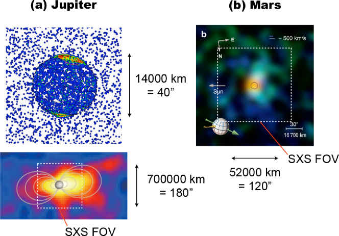
Figure 4: (a) X-ray images of Jupiter with Chandra HRC in 0.5–10 keV (Gladstone et al., 2002) and Jupiter’s inner radiation belts with Suzaku XIS in 1–5 keV (Ezoe et al., 2010a). In the bottom panel, solid lines indicate equatorial crossings of Jovian magnetic fields. An optical image of Jupiter is overlaid. (b) Soft X-ray image of Mars with XMM-Newton RGS (Dennerl et al., 2006). Colors indicate ionized oxygen emission lines in blue, ionized carbon lines in green, and fluorescence lines in yellow and red.

The ASTRO-H SXS opens up a new view of the planetary environments using the CX emission lines. We can directly distinguish fluorescent emission lines from the CX lines such as OVII K$\alpha$ in the Jupiter’s aurora and Martian exosphere, and can accurately determine line properties. Although grating observations have been conducted with XMM-Newton RGS and provided hints of what high energy resolution spectroscopy could achieve, the spatial extent of all solar system planets combined with the limited effective area of the RGS leads to significant uncertainties in the line properties. The SXS can achieve high energy resolution and high S/N at the same time because of its large effective area above 0.5 keV and anticipated low background.

Simultaneous observations with exploration satellites (JUNO, Mars Express) and solar wind monitoring satellites (ACE, WIND) will enable us to deduce the exospheric density from the observed X-ray line intensities, as demonstrated with Suzaku for Mars (Ishikawa et al., 2011). This will lead to an understanding of the not-well known exospheres.

From Doppler shift and broadening, dynamics of ions in the line of sight direction will also be constrained with SXS, since there are significant variations expected. In particular, the average speed of the solar wind particles ranges from $\sim$400 km to $\sim$700 km s^-1, while that of the precipitating ions accelerated by strong field aligned potential into Jupiter’s aurora is presumed as $\sim$5000 km s^-1 (Branduardi-Raymont et al., 2007).

The ASTRO-H SXI and HXI will allow us to detect hard X-ray continuum due to the inverse Compton scattering at the inner radiation belts and bremsstrahlung at the aurora. Hence, not only high energy ions but also electrons can be investigated from high sensitivity X-ray spectra.

Beyond Feasibility:

If the solar wind ion flux dramatically increases during a rare occasion such as a coronal mass ejection, the planetary CX emission can significantly increase. A TOO-type joint observation with solar wind monitoring satellites may make this rare detection feasible.

3.4 Geocoronal SWCX

Background and Previous Studies:

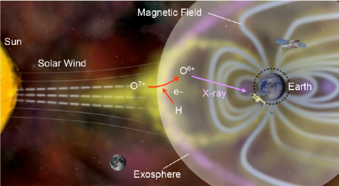
Figure 5: Schematic of geocoronal SWCX emission modeled after an illustration taken from http://chandra.harvard.edu/photo/2003/moon.

Solar wind charge exchange (SWCX) in the Earth’s exosphere, which is often called geocoronal SWCX, can constitute additional sources of diffuse time-variable background in astrophysical observations. Figure 5 shows a schematic of the process. The SWCX emission is in general composed of emission lines from highly ionized ions and mainly seen in the soft X-ray band ($<2$ keV). This emission was found during the ROSAT all sky survey as “Long Term Enhancements” (Snowden et al., 1994). A systematic search for the SWCX events has been done for the XMM-Newton and Suzaku archival data by Carter et al. (2011) and Ishikawa (2013), respectively. This unwanted background for general users can be a new tool to study the solar wind as well as the Earth’s exosphere and magnetosphere as demonstrated with Suzaku observations (Fujimoto et al. 2007; Ezoe et al. 2010b, 2011b). However, the high energy resolution spectroscopy has been impossible because the geocoronal SWCX is extended over the FOV of X-ray CCDs.

Prospects & Strategy:

For the first time with the ASTRO-H SXS, the high energy resolution spectroscopy will be possible for the geocoronal SWCX. In all SXS observations of astronomical objects, we can constrain the SWCX contribution directly from line distributions, since the CX is known to produce strong emission lines from large principle quantum number states and strong forbidden lines. The geocoronal SWCX can be separated from another SWCX background, i.e., the heliospheric SWCX using short term ($<$1 day) time variation because of its compact emission region ($\lesssim$tens Earth radii).

Combined with ACE and WIND data, the the solar wind ion fluxes can be obtained at the same time. The observed X-ray intensity will thus be able to be compared with a theoretical model considering an exospheric density model that gives the neutral distribution and a geomagnetic field model that defines the solar wind distribution. As suggested from Suzaku observations (e.g., Fujimoto et al. 2007), this comparison will provide us a clue of the shape of the magnetosphere, especially the location of the magnetocusp, which is recognized as one of the most important issues in space plasma physics.

From Doppler shift and broadening of individual emission lines detected in spectra, dynamics of ions will be constrained with an accuracy of several hundreds km s^-1. Solar wind abundances will be studied from the relative X-ray line intensities. Furthermore, since the geocoronal SWCX is the nearest CX source, it will provide us with fundamental information on CX such as line ratios and cross sections, that must be useful for extra-solar observations.

Targets & Feasibility:

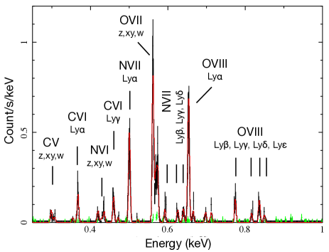
Figure 6: A 50 ks SXS simulation of the strong geocoronal SWCX event. Green shows a simulated 50 ks spectrum of SXB for comparison.

Because the geocoronal SWCX always exists as background emission in all ASTRO-H observations, a dedicated observation time is not necessarily needed. By carefully checking short time variability on the order of hr or day of emission lines and comparing the X-ray data with the solar wind data, we can pick up the SWCX event. By searching 6-yr Suzaku archive data for time variable geocoronal SWCX events, Ishikawa (2013) found that about $\sim$2 % data are affected by the geocoronal SWCX. The OVII line intensity, which is one of the most prominent lines in the SWCX, averaged over each observation, ranges from $\sim$3 to $\sim$50 Line Units (LU), where a LU is defined as a photon s^-1cm^-2sr^-1. From this study, we expect about 5 strong geocoronal SWCX events per year with the OVII line intensity more than $>$10 LU as long as the solar activity after launch (2015$\sim$16) is as high as that in 2005. This is highly likely considering the 11 yr cycle of the solar activity.

As an example, a 50 ks observation of the strong geocoronal SWCX event is simulated based on Ezoe et al. (2011b), in which the OVII line intensity was 34 LU, as shown in Figure 6. The exposure time corresponds to a typical duration of a large magnetic storm during which the solar wind flux significantly increases. The assumed SWCX model originally constructed by Bodewits et al. (2007) accounts for the relative emission cross sections for the lines from each of several ions. Emission lines from CV, CVI, NVI, NVII, OVII, and OVII are clearly detected. Although the solar wind ion abundance can change event by event, for strong emission line(s), the line center energy, width, shift and intensity can be determined with high accuracy of the order of $\sim$$\pm$1 eV and $\sim$10%.

For comparison, we simulated a 50 ks spectrum of the soft X-ray background (SXB) consisting the CXB component represented by an absorbed broken power-law function, and two thin-thermal emission components to represent the heliospheric SWCX induced emission lines plus Local Hot Bubble and Galactic emission from Yoshino et al. (2009). We can confirm that photons from the geocoronal SWCX dominate the data.

Beyond Feasibility:

Similar to the planetary CX emission, a TOO joint observation with solar wind monitoring satellites maybe possible to aim at detection of a extremely bright SWCX event. A blank sky region such as the north ecliptic pole will be proper as a line of sight direction, to avoid contamination from bright soft X-ray sources and to study the magneto-cusp region.

3.5 Comets

Background and Previous Studies:

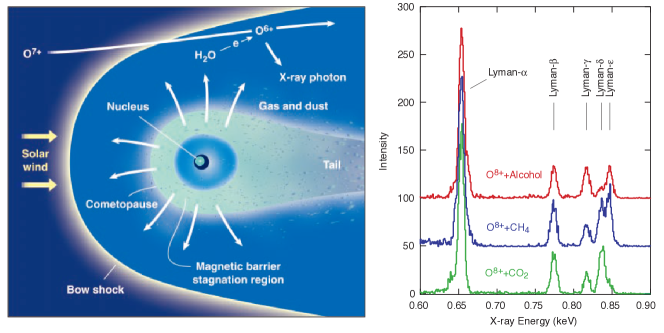
Figure 7: [Left] Schematic of cometary SWCX (Cravens et al., 1997). [Right] Laboratory experiment showing K-shell emission from O⁷⁺ after charge exchange with different molecules. (Beiersdofer et al., 2003).

The discovery of soft X-ray emission from Comet Hyakutake has revealed the existence of a new class of X-ray emitting objects, i.e., SWCX between the solar wind and neutrals (Lisse et al., 1996). A widely spread coma, whose size is 10^4-6 km and the number density ranges 10^0-8 molecules cm^-3 depending on the distance from the core of the coma (e.g., Lisse et al. 2003), emits X-rays via SWCX, as shown in Figure 7[left]. Since the comets are one of the brightest X-ray sources in the solar system, observational studies of the cometary X-ray emission must enable us to a better understanding of not only the cometary coma but also the SWCX process itself which is known to play an important role in other astrophysical objects.

Prospects & Strategy:

Similar to the geocoronal and heliospheric SWCX, for the first time with the ASTRO-H SXS, the high energy resolution spectroscopy will be possible for comets, since they are diffuse X-ray objects. Line properties such as Doppler shift, broadening if exists, and intensity will provide us with information on the dynamics of ion, the solar wind ion abundance, and the neutral density in the cometary coma, in the same way as the other SWCX sources.

A ground-based experiment using the ASTRO-E XRS spare detector revealed the potential for using cometary X-rays to infer information about the chemical composition of the cometary gases (Beiersdofer et al., 2003). The principal quantum number of electron capture changes with the ionization potential of the electron-donating material. Electrons will be captured into higher n-levels if the ionization potential of the donor electron is lower, resulting in different high n-level line distributions. The experimental result is shown in Figure 7[right].

Beyond Feasibility:

Similar to the other SWCX sources, a huge increase of the X-ray flux can be expected according to an increase of the incident solar wind associated with such as coronal mass ejection and co-rotational interaction region.

3.6 The “Beyond”

X-rays from CX may also be observable from more distant sources such as supernova remnants and galaxies. CX emission in SNRs are thought to play an enhanced role where neutrals are mixed with shocked hot gas. In fact, observational evidence of CX emission was found at optical wavelengths more than 30 yrs ago (e.g., Kirshner & Chevalier, 1978). In the X-ray domain, Wise & Sarazin (1989) first performed detailed calculations of CX-induced X-ray emission in a SNR. They found that CX emission generally contributes only 10^-3 to 10^-5 of the collisionally excited lines in the entire SNR. On the other hand, Lallement (2004) later examined projected emission profiles for both CX and thermal emission in SNRs, and noted that CX X-ray emission may be comparable with thermal emission in thin layers at the SNR edge. It is also pointed out that the relative importance of CX X-ray emission to thermal emission is proportional to a quantity, $n_{\mathrm{c}}$ $V_{\mathrm{r}}$ $n_{\mathrm{e}}^{-2}$, with $n_{\mathrm{c}}$ being the cloud density, with $V_{\mathrm{r}}$ the relative velocity between neutrals and ions, and $n_{\mathrm{e}}$ the electron density of the hot plasma. Thus, the higher the density contrast ($n_{\mathrm{c}}$/$n_{\mathrm{e}}$), the stronger the presence of CX X-ray emission would become.

There are growing observational hints of CX X-ray emission in SNRs, 1E0102.2–7219 in the SMC (Rasmussen et al., 2001), the Cygnus Loop (Katsuda et al., 2011) and Puppis A (Katsuda et al., 2012) in our Galaxy. The line intensity ratios of ($n>2\rightarrow n=1$)/($n=2\rightarrow n=1$) in H-like O (1E0102.2–7219) or He-like O (Cygnus Loop) seem to be higher than expectations from thermal emission models. In Puppis A, forbidden-to-resonance line ratios in He$\alpha$ transitions derived by the XM-Newton RGS spectra are found to be anomalously enhanced at the most prominent cloud-shock interaction regions. These could be naturally explained by the presence of CX emission, although other possibilities such as uncertainties on Fe L-shell lines, missing inner-shell satellite lines, and effects of resonance line scattering as well as recombination.

In star-forming regions, hot plasmas generated by massive stellar clusters can meet cold neutral gases, as they move through crevices of cold clouds. At the interfaces, highly-ionized ions in the hot plasma can interact with neutrals, and thus CX X-rays can be emitted. In fact, during the recent Chandra Carina Complex Project, it is noticed that the X-ray spectrum from a southern outflow in a giant HII region, NGC 3576, requires a Gaussian at 0.72 keV to obtain a good fit. This Gaussian component has been interepreted as CX X-ray emission (Townsley et al., 2011), although other possibilities are not yet ruled out, e.g., Fe L lines missing in the current plasma codes or something else due to previously-unrecognized physical processes.

By analogy to the star-forming regions, star-forming galaxies are also possible sites where CX X-ray emission can play an important role. A marginal detection of an emission line at 0.459 keV is reported for the starburst galaxy M82, which may be due to the CX emission of C VI (Tsuru et al., 2007). Stronger supports for the CX were later found in the line ratios of the O VII He$\alpha$ (Ranalli et al., 2008; Liu et al., 2011). Recent high-resolution X-ray spectroscopy with the XMM-Newton RGS has been revealing fine structures of O VII He$\alpha$ lines for a number of bright central regions of star-forming galaxies. For most cases, the forbidden lines are found to be comparable to or even stronger than the resonance lines (Liu et al., 2012). Together with the correlation with H$\alpha$ emission and the X-ray emission (e.g., Wang et al., 2001), this is best explained by significant contributions of CX emission. The CX X-ray emission may be ubiquitous for galaxies with massive star formation.

The non-dispersive spectrometer SXS on board ASTRO-H will allow for further tests for the CX scenario and other possibilities. The SXS is able to reveal spatial distributions of line intensity ratios such as forbidden-to-resonance in K$\alpha$ transitions and ($n>2\rightarrow n=1$)/($n=2\rightarrow n=1$) that are key information to find CX signatures in thermally-dominated X-ray emission. The CX scenario can then be examined by seeing if there are any spatial correlations between these lines ratios and the distance from the shock front and/or locations of optical clouds which could be electron donors. The SXS is also sensitive to other complex and/or faint spectral features such as radiative recombination continua, when compared with the RGS having smaller effective area and suffering from energy degradation due to the spatial extent of the source. In this way, the SXS will be essential to examine the possibilies of the CX X-ray emission in many astrophysical sites including SNRs, star-forming regions, and galaxies. Taking account of the CX emission would be extremely important for understanding the true properties of the shocked plasma, since the undetected presence of CX emission leads to incorrect plasma parameters (e.g., the metal abundance and the electron temperature) if we interpret the CX-contaminated X-ray spectra with pure thermal emission models. An SXS simulation for the Cygnus Loop SNR can be found in the ASTRO-H white paper (Knox et al. 2013).

4 Advanced Spectral Modeling: Photoionized and Collisional Plasmas

4.1 Background and Previous Studies

X-ray astronomy, particularly for bright sources, will change dramatically once high-resolution spectra from ASTRO-H become available. We will encounter a number of unexpected spectral features with unprecedented statistics. In such cases, the simple method of ‘chi-squared fitting’ (relying on canned spectral models with a small number of parameters) will no longer return reliable results, and requiring an advanced modeling effort.

Unexpected spectral results have already been obtained even with recent moderate-resolution data with Suzaku, taking advantage of deep observations with low background. The discovery of strong radiative recombination continua from collisionally-ionized plasmas (Yamaguchi et al., 2009; Ozawa et al., 2009) as shown in Figure 8a was one of the most surprising results concerning supernova remnants (SNRs), has and significantly changed our understanding of SNR’s dynamics and evolution (see also the Old SNR WP). Suzaku’s low-background and good resolution has also enabled us to detect low- abundance elements (e.g., Al, Cr, Mn, Ni) and weak emission lines from more abundant elements (e.g., Fe K$\beta$), providing useful diagnostics of the progenitor’s nature (e.g., Badenes et al., 2008) and ion population in plasmas (Yamaguchi et al. 2013, see Figure 8b and its caption). It is notable that most of these spectral features were not predicted by any public model at the time of the discoveries. This is a key point: Do not rely too much on prepared spectral models someone else made! There is no model free of assumptions, limitations, or applicable ranges. The high- resolution data of ASTRO-H will, more than often, show unexpected and important features, and a shift to an advanced modeling approach based on a knowledge of fundamental atomic physics will be needed. Otherwise, we may overlook important signatures that the observational data will be telling us. For example, although new SWCX models are now available, they are only applicable in specific circumstances; applying them without care will lead to unphysical results that cannot be justified even if they fit parts of a spectrum.

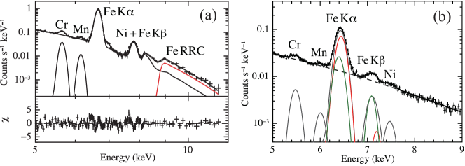
Figure 8: (a) Suzaku spectrum of W49B (Ozawa et al. 2009). The red line represents the strong RRC of He-like Fe, which can be enhanced only when the plasma is overionized.  (b) Suzaku spectrum of the NW rim of Tycho (Yamaguchi et al., 2014). The K$\alpha$ and K$\beta$ emission lines of Fe are successfully reproduced by a ‘two-component’ model consisting of low-ionization (around Fe⁸⁺: green) and higher-ionization (around Fe¹⁶⁺: red) components. The K$\beta$/K$\alpha$ ratios of the former and latter are assumed to be 0.15 and 0.01, respectively. The low ratio for Fe¹⁶⁺ is expected because there is no bound electron in the $3p$ shell. The detailed values of the centroids and intensity ratio for each charge stage is given in Table 1.

4.2 Non-Equilibrium Ionization and Ion Population

In this and the next subsections, we discuss collisionally-ionized plasmas where both excitation and ionization by UV/X-ray photons are negligible. At an X-ray-emitting temperature, heavy elements in plasmas are highly ionized, usually to He-like or H-like state (except for the heaviest abundant elements such as Fe and Ni). This is because the internal kinetic energy of electrons are comparable to the K-shell ionization potential of the astronomically-abundant heavy elements (i.e., C through Ni). Figure 9a shows the ion population of Fe as a function of electron temperature $kT_{e}$, assuming ionization equilibrium (CIE). In a CIE plasma, the fractional abundance of each ion can be determined uniquely by $kT_{e}$, so spectral analysis is relatively straightforward — just applying a simple CIE plasma model (e.g., apec: Smith et al. (2001); Foster et al. (2012); mekal: Mewe et al. (1985); Kaastra (1992)) would be fine (but we should still be careful about uncertainty and limitation in the atomic data). The assumption of CIE is fulfilled in a majority of astronomical X-ray emitting plasmas, such as galaxy clusters.

However, the situation is more complicated when the physical condition (e.g., temperature) of the plasma suddenly changes and the timescale of the temperature fluctuation is shorter than that required to reach CIE. Such an unsteady condition is called “Non-Equilibrium Ionization (NEI)”. An NEI plasma is commonly observed in SNRs as they form shock waves heating ISM or supernova ejecta up to high temperature abruptly. The degree of NEI is quantified by “ionization age” parameter $\tau=n_{e}t$, a product of electron density ($n_{e}$) and elapsed time since the sudden temperature change ($t$). The timescale to reach CIE depends on the electron temperature and element, and is typically in a range of $n_{e}t=10^{10}-5\times 10^{12}$ cm^-3 s (e.g., Smith & Hughes, 2010). Figure 9b gives ion fraction in a $kT_{e}=5$ keV ionizing NEI plasma as a function of $n_{e}t$. The ion population calculated for an ionizing plasma largely differs from that in a CIE plasma. As expected, the charge number of the ions is very low (almost neutral) in the early NEI stage and gradually goes up as the $n_{e}t$ value increases. It is worth noting that, in the CIE plasma, the abundance curve of the Fe¹⁶⁺ (Ne-like) ion shows a ‘plateau’ (relatively flat region) at $\sim$0.3–0.6 keV, while those of the non-closed-shell ions (e.g., Fe¹²⁺, Fe²⁰⁺) have a steeper peak. In the ionizing plasma, on the other hand, the shape of the Fe¹⁶⁺ abundance curves looks very similar to those of the other ions. This can be more quantitatively presented in Figure 10. This shows the standard deviation of a charge number $\sigma=[\Sigma_{i=0}^{26}\,f_{i}\,(z_{i}\,-\,$$<$$z$$>$$)^{2}]^{1/2}$ in both cases, where $f_{i}$, $z_{i}$ and $<$$z$$>$ are the fraction and charge number of Fe ion (Fe${}^{z{{}_{i}}+}$) and the average charge, respectively. Unlike the CIE case, relatively flat deviations are achieved throughout the evolution of the ionizing plasma.

The ion populations expected for a recombining plasma are strikingly different from those in the CIE and ionizing plasmas. Figure 9c demonstrates evolution of a $kT_{e}=0.3$ keV recombining plasma assuming that the initial ionization balance corresponds to a 30 keV CIE plasma. Interestingly, the fully-stripped and Ne-like ions can co-exist during a certain evolutional stage (which cannot happen either in the CIE or ionizing case), and also the standard deviation is expected to be much larger than those in the other cases (Figure  10). Such a broad distribution of different ions can be achieved because the recombination rate does not strongly depend on the charge number, in contrast to the ionization rate.

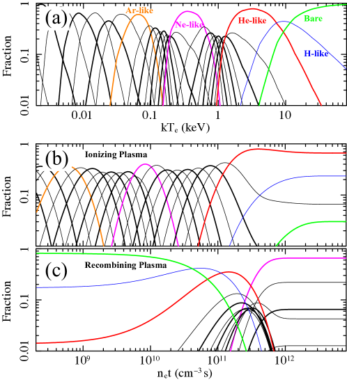
Figure 9: (a) Ion population of Fe in a CIE plasma as a function of the electron temperature. Orange, magenta, red, blue, and green represent Fe⁸⁺ (Ar-like), Fe¹⁶⁺ (Ne-like), Fe²⁴⁺ (He-like), Fe²⁵⁺ (H-like), and Fe²⁶⁺ (fully-stripped), respectively.  (b) Ion population of Fe in an $kT_{e}=5$ keV ionizing plasma as a function of the ionization age.  (c) Same as (b), but for recombining plasma where the initial and current electron temperatures are assumed to be 30 keV and 0.3 keV, respectively.

The difference in the expected ion population among the different plasma states (i.e., CIE, ionizing, recombining) becomes rather important when we introduce a physical quantity, “ionization temperature ($kT_{z}$)” which can be defined for a particular ionization distribution as the temperature such that the average charge of the ionization distribution is consistent with that of a CIE plasma with electron temperature $kT_{z}$. We should note, however, that although the average charge of the ion population of a $kT_{z}=1$ keV recombining plasma is by definition identical to that of a $kT_{e}=1$ keV CIE plasma, the overall ion distribution will be hugely different. Moreover, in realistic ionizing or recombining plasmas, an electron temperature also evolves with time and both $kT_{e}$ and $n_{e}t$ have spatial non-uniformity. Therefore, ion population in the realistic sources will be not as simple as the simple NEI models predict. In fact, it was found that the Suzaku spectrum of Tycho (Figure 8b) cannot be represented by a single-component NEI or parallel-shock model (; see the Young SNR WP for more detail Yamaguchi et al., 2014). Future spectral analysis especially for high-resolution data should, therefore, be more flexible so that an arbitrary ion population can be described.

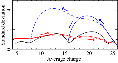
Figure 10: Standard deviation of a charge number vs average charge for a CIE (black), ionizing (red), and recombining (blue) plasmas.

4.3 Innershell Process and Fluorescent X-Ray Emission

Innershell ionization/excitation processes are particularly important for high-$Z$ elements in young SNRs, since their ionization stage is usually observed to be lower than the He-like state. Nonetheless, there is currently no public model that completely includes these processes due to a inadequate atomic data. Figure 11 compares model spectra of an NEI plasma with $n_{e}t$ of $2\times 10^{10}$ cm^-3 s predicted by XSPEC, SPEX, and a more accurate calculation using the “Flexible Atomic Code (FAC)” (Eriksen et al., 2013). The most obvious difference is seen in the energy range between 7 and 8 keV. We find neither the XSPEC nor SPEX NEI models include any K$\beta$ emission except for He-like and H-like states. The energy (wavelength) of K$\alpha$ emissions in the existing models is also found to be inaccurate; for example, all the K$\alpha$ emissions of Fe II–XII and Fe XIII–XVII are placed at 6390 eV and 6425 eV, respectively, in SPEX (see Table 1 for comparison with the accurate values), while the XSPEC NEI model obviously oversimplifies the line profiles as shown in Figure 11a. In order to determine accurate ionization ages, abundances, and ion temperatures, accurate predictions of the line energy and emissivity is essential. Table 1 gives the centroid energies of the Fe K$\alpha$ and K$\beta$ emissions and their intensity ratio for different charge numbers at $kT_{e}=5$ keV. We emphasize that the modeling of K$\beta$ emission is particularly important because: (1) the centroid energies of the Fe K$\beta$ lines are well separated from those of the next charge stages, compared to the Fe K$\alpha$ lines, which will be an advantage when measuring ion fractions and thermal-Doppler line widths (see Figure 11c). (2) the K$\beta$/K$\alpha$ intensity ratio is sensitive to the charge state, and thus a diagnostic of the ion population (Yamaguchi et al., 2014, ; see also the Young SNR WP). Since the K$\beta$/K$\alpha$ ratio becomes higher than 10% at $z\leq 10$, clear detection of K$\beta$ emission is expected from most SNRs with low-ionized Fe ejecta (e.g., Tycho, Kepler, SN1006, Type Ia SNRs in the LMC). For highly-ionized Fe ($14\leq z\leq 18$), on the other hand, the ratio goes down to $\lesssim 2$%. However, their contribution is still the subject of consideration, because their line energies overlap with those of Ni-K$\alpha$ emission (which is also weak compared to Fe-K$alpha$ lines). The accurate Fe-K$\beta$ data will, therefore, help accurate measurement of Ni abundances.

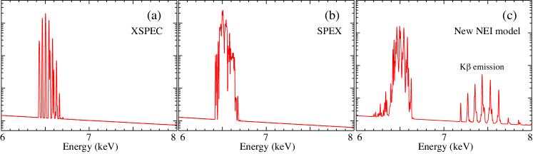
Figure 11: Comparison of model spectra for an ionizing plasma with $n_{e}t=2\times 10^{10}$ cm^-3 s, predicted by XSPEC, SPEX, and detailed calculation using the “Flexible Atomic Code” (Eriksen et al., 2013). No K$\beta$ emission is involved in XSPEC or SPEX despite its importance for diagnostics.

$z$	$E_{{\rm K}\alpha}$ (eV)	$E_{{\rm K}\beta}$ (eV)	K$\beta$/K$\alpha$ ratio		$z$	$E_{{\rm K}\alpha}$ (eV)	$E_{{\rm K}\beta}$ (eV)	K$\beta$/K$\alpha$ ratio
0	6402	7059	0.120		12	6415	7144	0.063
1	6402	7060	0.121		13	6420	7158	0.036
2	6402	7060	0.122		14	6420	7153	0.015
3	6401	7059	0.127		15	6425	7176	0.010
4	6400	7063	0.132		16	6427	7192	0.012
5	6399	7070	0.136		17	6455	7270	0.009
6	6399	7075	0.141		18	6484	7351	0.013
7	6399	7081	0.149		19	6517	7434	0.025
8	6398	7090	0.168		20	6544	7517	0.029
9	6401	7102	0.146		21	6575	7610	0.036
10	6405	7116	0.122		22	6589	7705	0.044
11	6410	7128	0.099		23	6641	7777	0.075

Table 1: The centroid energies of Fe-K$\alpha$ and K$\beta$ emissions and their intensity ratios for the different charge numbers $z$. For $z=9-13$, only K-shell ionization (and no excitation) is taken into account, so the centroids are slightly overestimated and the ratios are underestimated. More detailed information/values will be found in Yamaguchi et al. (2014).

Innershell ionization of Li-like ions frequently creates the excited $1s2s$ state, and hence can significantly contribute to the formation of the He-like forbidden line. Therefore, not only the $G$ ratio ($\equiv(x+y+z)/w$) but also the $R$ ratio ($\equiv z/(x+y)$) is expected to be enhanced (e.g., Mewe & Schrijver, 1985). This provides a useful diagnostic to distinguish the innershell effect from other processes that can also induce the forbidden transition (i.e., radiative/dielectronic recombination and charge exchange). Both the recombination and charge exchange processes favor the populations of the triplet levels, due to their higher statistical weight compared to the singlet level. Therefore, the intercombination lines will also be enhanced, resulting in a smaller $R$ ratio.

Most (probably all) of the public NEI codes use values of fluorescence yields ($\omega\equiv A_{r}/(A_{r}+A_{a})$, where $A_{r}$ and $A_{a}$ are radiative and Auger rates, respectively) calculated by Kaastra & Mewe (1993). This work used a single-configuration approach in order to keep the calculation to manageable size for the time and thus several important effects, such as configuration interaction, were ignored. It has been pointed out that this simplification can be problematic in some situations (e.g. Gorczyca et al., 2006). One of the most significant cases is seen in the Li-like $1s2s^{2}$ state (after innershell ionization of a Be-like ion). Since this excited state contains no $2p$ electron, a permitted (electric dipole) transition is impossible. Therefore,Kaastra & Mewe (1993) gave $\omega=0$ for every Li-like ion. However, once the configuration interaction effect is taken into account, the yields will have non-zero values due to mixing with a $1s2p^{2}$ wave function. This effect becomes prominent especially for high-$Z$ elements. For example, the yield was found to be $\sim$0.12 for $1s2s^{2}$ Fe²³⁺ (Gorczyca et al., 2006), so the fluorescent emission significantly contributes to a spectrum. As an example, this amounts to $\sim 10\%$ increase in the Li-like line flux for $n_{e}t=7\times 10^{10}$ cm^-3 s where Be-like Fe is dominant. We should, therefore, properly take into account these effects in order to obtain an accurate prediction of the satellite line profile.

In addition to the inner K-shell ionization and fluorescence, L-shell fluorescence could also be important for low-ionized plasmas. The current plasma models are designed to have Fe L-shell emission only above Fe¹⁶⁺. This is because at typical X-ray-emitting temperatures ($>0.2$ keV), the population of Fe¹⁵⁺ and lower-charged Fe is almost negligible (Figure 9a). However, this is not the case for an ionizing plasma with an extremely low ionization age ($n_{e}t<5\times 10^{9}$ cm^-3 s; see Figure 9b), and thus there is no reason that we ignore the L-shell emissions from the lowly-charged Fe. A comprehensive model that includes these missing lines should be established for high-resolution spectroscopy with ASTRO-H.

4.4 Photoionized Plasma

As well as the collisional ionization discussed above, photoionization is an important process that drives X-ray emitting plasmas. Photoionized plasmas driven by X-rays, which are commonly seen around accretion-powered objects such as neutron stars and black holes including active galactic nuclei (AGN), reveal the physical conditions of the surroundings of the energetic objects through complicated spectra containing a number of emission or absorption lines. This information will play a key role in revealing how the accretion power affects the surrounding environment, leading to the knowledge of the evolution of galaxies (See AGN chapter). However, modeling of the photoionized plasma is highly complex since the physical conditions of the plasma cannot be determined purely by local properties. As the plasma is driven by an external X-ray source, the geometrical relation to the source and even to other parts of the plasma must be considered.

To calculate the spectrum of a photoionized plasma, there are three steps to obtain the results:

1. understand physical processes from a microscopic viewpoint;

2. determine physical states of the plasmas; and

3. calculate radiative transfer.

For the first item, we need models of emissions and photon interactions with ions based on atomic physics and precise atomic data. The basic points of this problem should be common to those for the thermal plasmas discussed in the previous subsections. Nevertheless, the difference in the efficiency of atomic processes is worthy of attention. For example, in photoionized plasmas, dielectronic recombination is negligible in many cases since radiative recombination is much more efficient at low temperature than dielectronic recombination. Such a disregard simplifies the calculation of the ionization balance in the next step. The second step is to determine hydrodynamical structure of the plasma including temperatures, densities, velocities, and ion abundances (chemical compositions and ion fractions). Although these properties can be all coupled, it is usually sufficient to calculate the distributions of ion fractions and temperatures by balancing ionization and recombination, and also balancing heating and cooling with the assumption that other hydrodynamical properties such as the density distribution can be fixed. The third step gives the resultant emission from the plasma. Since the radiative transfer also affects the photoionization and photoexcitation processes, the second and third steps are strongly coupled, and the problem should be solved self-consistently. Many photoionization calculating codes, e.g. XSTAR (Kallman & McCray, 1982), CLOUDY (Ferland et al., 1998), have adopted iterative algorithms to obtain the final solution.

As the problem of radiative transfer is a major issue in astrophysics, we discuss it separately in the next section, and here we briefly describe a strategy. If the system is optically thin, the degree of photoionization is easily characterized by a ionization parameter $\xi$ defined as

$$\xi=\frac{L_{X}}{n_{e}r^{2}}=\frac{4\pi F_{X}}{n_{e}},$$ (5)

where $L_{X}$, $n_{e}$, and $r$ denote the X-ray luminosity of the source, the electron density, and the distance to the source, respectively. This parameter controls the ionization balance since the ionization and recombination rates are proportional to the ionizing flux $F_{X}$ and the electron density $n_{e}$, respectively. When the system becomes optically thick, one-dimensional radiative transfer in a simplified geometry such as plane-parallel geometry or spherical geometry provides an effective approach. In more complicated case, a Monte Carlo simulation would be preferred (Watanabe et al., 2006; Sim et al., 2008).

Photoionized stellar winds in high-mass X-ray binaries (HMXBs) provide ideal laboratories for study of physics of photoionized plasmas (see HMXB chapter). Watanabe et al. (2006) analyzed Chandra grating spectra of Vela X-1 and modeled the spectra by using Monte Carlo simulations. Figure 12 shows ion distributions of Si XIV in the binary system, which were calculated by using XSTAR, assuming a standard stellar wind model by Castor et al. (1975). Then, using these ion distributions, they performed the Monte Carlo simulation that carefully treats photoionization and photoexcitation, as well as Compton scattering. In this framework, resonance scattering is naturally included in a process of photoexcitation followed by a radiative decay. As shown in Figure 13, the simulation reproduced the observed data with a mass-loss rate of $1.5\times 10^{-6}\ M_{\odot}\ \mathrm{yr}^{-1}$. This approach, using detailed Monte Carlo simulations, will be applicable to a wide variety of astrophysical objects including AGN outflows (e.g. Evans et al., 2010; Detmers et al., 2011; Tombesi et al., 2010).

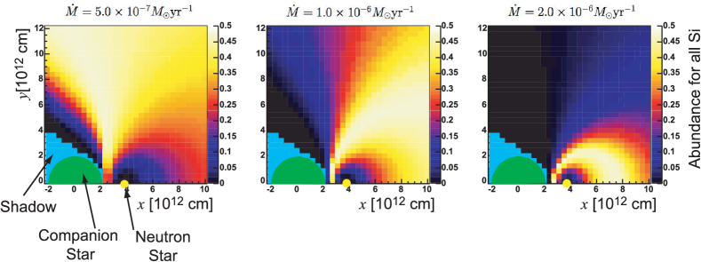
Figure 12: The ion fraction maps of Si XIV (H-like) in the Vela X-1 system for different mass-loss rates $\dot{M}$ of the B-type donor star (Watanabe et al., 2006).

Figure 13: Comparison of the simulated spectra of Vela X-1 with the observed data for three different orbital phases (Watanabe et al., 2006). The normalization of the simulation models is fixed between the three phase ranges, assuming that the average X-ray luminosity does not change.

5 Radiative Transfer (including Compton Scattering)

5.1 Introduction

The unparalleled high-quality data obtained with ASTRO-H will require accurate and precise astrophysical interpretation. In addition to the detailed treatment of the emission processes described in the previous section (§4), the modeling of electromagnetic radiation from astrophysical objects can involve solving problems of radiative transfer, since the emitted radiation may be altered by absorption as well as scattering. A variety of methods for the radiative transfer problems have been developed; the selection of approaches depends on physical situations of the problem, required accuracy, and/or convenience of astrophysicists (and sometimes on their preference).

The optical thickness of astrophysical system is the most important physical quantity that characterizes the problem. If the system is optically thin, the problem becomes straightforward. For optically thick systems, we usually describe the problem by a partial differential equation where a continuous approximation is introduced, and then solve it analytically or numerically. Particular difficulties lie in the intermediate situation, namely, an optical depth about 0.5–10. Since in this case individual reprocessing of photons by matter has significant effects on the resultant emission, we have to treat the discontinuity of the photon processes, competing processes, and multiple interactions. Moreover, the geometry of the system, which can be complicated, should be taken into account.

5.2 Monte Carlo Approach

One of the standard approaches to the problems of radiative transfer is applying the transfer theory, which is based on the concept of a “ray” as a good approximation of radiation (Rybicki & Lightman, 1979). Introducing a specific intensity $I_{\nu}$ as the radiative energy propagating in a certain direction within a unit solid angle crossing unit area per unit time per unit frequency, the radiative transfer equation is formalized as

$$\frac{dI_{\nu}}{ds}=-\alpha_{\nu}I_{\nu}+j_{\nu},$$ (6)

where $ds$ is a small length along the ray, $\alpha_{\nu}$ is the absorption coefficient, and $j_{\nu}$ is the emission coefficient. This equation has a more general form that can treat time dependence and multi-dimensional space coordinates.

For the radiative transfer of X-rays, however, it is more useful in many cases to treat the radiation as photons. In this approach, the radiation can be calculated by a full photon tracking simulation based on a Monte Carlo method – aka, a “Monte Carlo simulation.” This method provides a natural description of the problems particularly for the systems with intermediate optical depths, since the discrete nature of the photon processes is automatically involved, and the complexities of the photon interactions mentioned above can be easily handled.

The simulation calculates the propagation and interactions of the tracked photon with matter. These are performed in two steps as shown in Figure 14. First, after a photon starts from a certain initial point, the next interaction position is sampled from an exponential distribution characterized by a mean free path,

$$l=\frac{1}{\sum n_{i}\sigma_{i}},$$ (7)

where $n_{i}$ and $\sigma_{i}$ are the number density of a target and the cross section of a process labeled by $i$, respectively. A process that occurs at the determined position is selected from among all competing processes by a probability proportional to $n_{i}\sigma_{i}$. Second, when the process occurs at the interaction position, the photon is absorbed or scattered. If it is absorbed, one or more photons can be reemitted through a certain process such as radiative decay. If it is scattered, the energy and direction are changed according to a differential cross section. While tracking, these two steps are applied repeatedly until the photon is absorbed or escapes from the system. The final interaction point before the escaping is recorded as an emission seen by an observer.

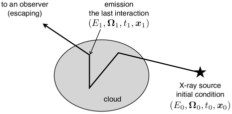
Figure 14: A schematic procedure of the Monte Carlo simulation (Odaka, 2011). In one tracking trial, the photon is generated at the X-ray source, and then it is tracked until escaping from the system. The final interaction point can be regarded as an emission by an observer. The initial and final points should be recorded for a following analysis of the simulation result.

5.3 X-ray Reflection and Compton Shoulder

When matter is illuminated by X-rays, we can observe X-rays reprocessed via photoelectric absorption followed by fluorescence, or Compton scattering. This phenomenon is called X-ray reflection. The X-ray reprocessing in cold matter provides us with an important probe of the structure, dynamics and chemical composition of the irradiated cold matter such as molecular clouds, dense gases in X-ray binaries, or torus-like structures around AGN. The reprocessed emissions also bring us fruitful information about the X-ray sources—black holes, neutron stars, or other energetic objects. This information becomes indispensable when we need to know the past activity of the illuminators by observing the delayed light via the reflector. If the distance between the illuminator and the reflector is small, the illuminated matter gets ionized and spectral modeling becomes more complicated. The reflection from ionized matter has been modeled in a context of reflected X-rays from accretion disks around black holes (Ross & Fabian, 2005; Garcia et al., 2010).

The reflection spectrum features a wide-band scattered continuum that has a hump at $\sim$20 keV (known as the “Compton hump”) as well as fluorescent lines from the abundant heavy elements. In addition, if the reflecting cloud is not optically thin, scattering of fluorescent line photons in the cloud forms a low-energy tail structure at the corresponding fluorescent lines. This spectral feature, called a Compton shoulder, contains information about the scattering medium. Figure 15 shows the spectrum of the high-mass X-ray binary GX 301-2 obtained with Chandra HETG, clearly displaying Compton shoulders around 6.2–6.4 keV of iron K$\alpha$ lines. By comparing the observed spectra and results of a detailed Monte Carlo simulation, Watanabe et al. (2003) constrained physical conditions of the scattering medium in the binary system including the electron temperature, column density, and the metal abundance.

Figure 15: Spectra of GX 301-2 from 5 to 10 keV obtained with Chandra HETG for the first and second halves of the observation (Watanabe et al., 2003). The solid lines show the Monte Carlo models inferred from the data. In addition to the iron Ka emission line profile, the continuum shape is also successfully reproduced with the parameters inferred from the Compton shoulder profile. The values for $N_{\mathrm{H}}$ are $12.0\times 10^{23}\ \mathrm{cm}^{-2}$ and $8.5\times 10^{23}\ \mathrm{cm}^{-2}$ for the first and second halves, respectively.

Since the X-ray reflection is widely seen in the Universe, it has been important to develop a calculation method of the spectrum and morphology. Murakami et al. (2001) developed a three-dimensional model of giant molecular cloud Sagittarius B2 (Sgr B2), and compared its morphology with an image of the iron line obtained with Chandra. Sgr B2 is thought to be reflecting X-rays originated from a past outburst of the supermassive black hole Sgr A* at the Galactic center (GC). Hamaguchi et al. applied a similar approach to an X-ray reflection nebula in the $\eta$ Carinae complex to obtain its spectrum and time variability of the emission. X-ray emission from the supermassive star, $\eta$ Carinae, is reflected, or absorbed and reemitted, at the surrounding bipolar nebula called the Homunculus nebula. The nebula glows in X-rays and can be recognized in high-resolution images with Chandra when strong X-ray emission from the central binary system plunges at around its periastron passage for a couple of months (Corcoran et al. 2004). In a series of Chandra observations during the X-ray minimum phase in 2009, the glow gradually faded as expected in a simulation of X-ray reflection from the central binary system at the Homunculus nebula, as shown in Figure 16. The observed spectra showed a broad line at  6.5 keV with a very high equivalent width of  2 keV. The line can be reproduced by iron fluorescence plus Compton down scatter of the Helium-like iron line in the incident spectra at the nebula.

Figure 16: X-ray reflection light curve of the HN (blue points: 2003, red points: 2009) and the best-fit of the light curve to a time-delay reflection model using the observed RXTE light curve of the central binary system (blue and red solid lines) (Hamaguchi). The horizontal axis shows the orbital phase of the central binary system.

In the ASTRO-H era, we will obtain more detailed information about the X-ray reflection. The microcalorimeter will measure fine spectral structures such as the Compton shoulder, absorption edges, and line shift and broadening due to the dynamical motion including turbulence. Moreover, imaging spectroscopy of hard X-rays above 10 keV enables probing of the deep regions in illuminated clouds owing to their large penetrating power compared with that of soft X-rays. Modeling the hard X-rays will also require accuracy since the hard X-ray photons may experience multiple scattering in the dense clouds, introducing complexity to the radiative transfer.

To handle this problem, a Monte Carlo approach that includes accurate physical processes and realistic geometry is the most suitable though it is sometimes time-consuming. Several authors have been adopted Monte Carlo simulations for modeling the X-ray reflection (Leahy & Creighton, 1993; Sunyaev & Churazov, 1998; Fromerth et al., 2001). Odaka (2011) also developed a multi-purpose framework (called MONACO) to calculate X-ray reprocessing based on a Monte Carlo simulation. This calculation includes detailed treatment of photoelectric absorption and scattering by electrons bound to hydrogen molecules and helium atoms (Sunyaev & Churazov, 1996). The scattering by a bound electron makes a difference in the spectral shape of the Compton shoulder from Compton scattering by free electrons—an effect that will often be evident in the SXS spectrum.

By using the MONACO framework, Odaka et al. (2011) calculated the X-ray reflection from Sgr B2 for several different models of the cloud structure, and predicted high-resolution spectra and hard X-ray morphologies, which can be observed by ASTRO-H as shown in Figure 17. Interestingly, the morphology of scattered hard X-rays above 20 keV is significantly different from that of iron fluorescence due to their large penetrating power. High-resolution spectra provide quantitative evaluation of the iron line including its Compton shoulder, constraining the mass and chemical composition of the cloud as well as the luminosity of the illuminating source. Such careful modeling will be necessary to extract physical parameters of the cloud itself and the central black hole from the high-quality data. A large-scale view of X-ray reflection from molecular clouds in the GC region will reveal the structure of the GC molecular zone and the history of the activity of the central black hole in our Galaxy.

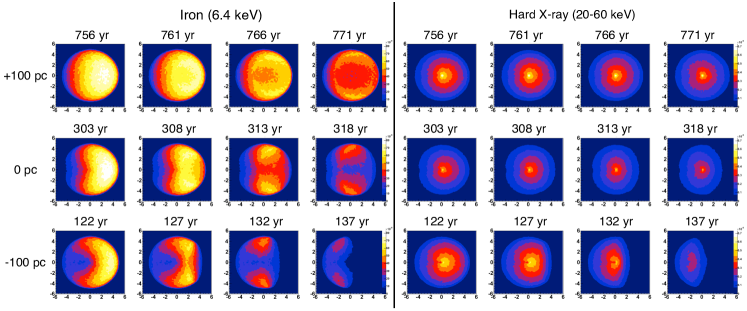
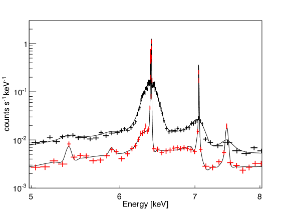
Figure 17: Calculated morphologies (top) and spectrum (bottom) of the X-ray reflection from Sgr B2 (Odaka et al., 2011). The top panel shows the time evolution of the morphology for different energy ranges (left: iron 6.4 keV line; right: 20–60 keV) from the brightest moment at intervals of five years. The observation time is marked at the top of each image and the cloud position along the line of sight is marked at the left of each row ($t=0$ is the moment of the end of the outburst). The bottom panel shows observation simulations of Sgr B2 with ASTRO-H SXS (red points) and Suzaku XIS 0+3 (black points) for an exposure time of 200 ks. The flux is assumed to be a value in the fading phase, namely 15 years after the brightest moment.

X-ray reflections in the vicinity of AGN contains important information on the structure and physical conditions of the environment around supermassive black holes (See AGN reflection chapter of this White Paper). Since the reflector, which is commonly referred to as an AGN torus, can be Compton-thick, Monte Carlo simulations are effective for accurate modeling that allows us to compare high-precision data obtained with the SXS and HXI. A set of numerical data tables called MYTorus (Yaqoob, 2012), which is generated by Monte Carlo simulations, is useful for detailed modeling of obscured AGN.

5.4 Photon Reprocessing in X-ray Emitting Plasmas

The reprocessing of photons can also have an impact on a spectrum emerging from an X-ray emitting plasma. Photons generated in the plasma can interact with electrons, atoms, or ions in the same plasma, altering the source function of the spectrum into other forms. If the assumption that the plasma is optically thin breaks, we should consider effects of radiative transfer. In this case, the Monte Carlo simulation allows us to construct precise models or to evaluate systematic uncertainties due to simplifications or assumptions of other fast models.

Photoionized Plasmas

As discussed in §4.4, radiative transfer plays a significant role in generating a spectrum of a photoionized plasma. For a photoionized plasma with complicated structure (e.g. stellar winds), the Monte Carlo simulation would be the most suitable approach. In Figure 18, we show an effect of turbulence on the spectrum of Vela X-1 calculated by the simulation. Turbulence suppresses resonance-Auger destruction(Ross et al., 1996; Liedahl, 2005), resulting in enhancement of resonance lines.

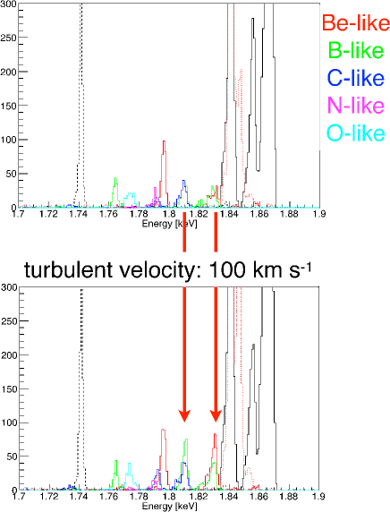
Figure 18: The two spectra show difference in line emissions due to turbulent velocity (Odaka, 2011). This is the first attempt to reproduce Si-K complex of Vela X-1 spectrum obtained with Chandra though model parameters are not optimized yet. Contributions of each Si ions to the Si K-line complex are obtained by the simulation: Si XIV (black dotted), Si XIII (black solid), Si XII (red dotted), Si XI (red solid), Si X (green), Si IX (blue), Si VIII (magenta), Si VII (cyan), and Si I–VI (black dashed). Photon counts are represented in arbitrary units.

Resonance Scattering

Plasma diagnostics based on high-resolution spectroscopy with the SXS will open a new window to investigate physical properties (i.e. spatial distributions of velocity, temperature, or density) of hot X-ray emitting plasmas in the universe, such as clusters of galaxies, supernova remnants, and star forming regions. These plasmas are driven by collisional ionization and can be regarded as optically thin. (Collisional ionization equilibrium is not necessarily achieved in some cases such as supernova remnants or merging clusters). At energies of resonance lines, however, the optical depth of the plasma can be close to unity or larger, resulting in distortion of the line spectrum. This process affects, for example, shape of the line profile or intensity ratios between triplet lines of helium-like ions. These effects by resonance scattering are sensitive to a velocity field of both bulk and random motions of the gases. Therefore, they can be probes of gas dynamics including turbulence, which is believed to be one of the major forms of non-thermal energy in the Universe. The effects of resonance scattering on the plasma diagnostics can be simulated by careful treatment of radiative transfer (e.g. Monte Carlo simulations) (Zhuravleva et al., 2010).

Comptonization

Inverse Compton scattering by hot electrons or non-thermal electrons can be also considered as photon reprocessing in a plasma. Thus, Comptonization, which is a result of multiple scatterings, can be calculated by the photon tracking simulation. Though it is well known that the Kompaneets Equation or its extension gives the solution of Comptonization, Monte Carlo simulations become a suitable approach if the system has complicated geometry or is not thick enough for modeling by the differential equation. The simulation is also advantageous when the physical process is more complicated in the presence of a strong magnetic field, which introduces birefringence to photons and cyclotron resonance effects.

6 Nuclear Lines, Annihilation Emission, and Solar Particle Acceleration

6.1 Introduction

Spectral line features, primarily resulting from nuclear transitions, are present in the hard X-ray and $\gamma$-ray bands and detecting these will be the goal of many ASTRO-H/HXI and SGD observations. In particular, the SGD will allow us to search for line emission in the soft $\gamma$-ray band from $\sim 80$ keV up to $\sim 600$ keV with unprecedented sensitivity. For example, INTEGRAL/SPI detected a strong electron-positron annihilation line at 511 keV from the direction of Galactic Center (GC) (Jean et al., 2003). The SGD will enable us, for example, to search for not only long-term but also short-term variabilities from this promising source in the 511 keV line thanks to its improved sensitivity. In addition, the radioactive decay of unstable isotopes synthesized during both supernova (SN) and nova explosions produces line features in the hard X-ray and $\gamma$-ray bands. In Table 1, we tabulate radioisotopes which emit line features in the energy ranges covered by the HXI and SGD (Diehl & Timmes, 1998).

Electron orbiting in a strong magnetic field have quantized energies, as do the X-rays that can be absorbed by these electrons. These absorption features, known as cyclotron resonance scattering, have been observed in the hard X-ray spectra of some of neutron star X-ray binaries (e.g., Mihara, 1995; Makishima et al., 1999), and they can be investigated by ASTRO-H/HXI. In addition, it is expected that solar flare neutrons are detectable by SGD. In the following, we describe the expected scientific results as well as potential ASTRO-H/HXI and SGD targets which should show line features in the hard X-ray and $\gamma$-ray bands.

6.2 Nuclear lines

Scientific Context

Type Ia SNe, thermonuclear runaway explosions of white dwarfs in binary systems, synthesize huge amounts of ⁵⁶Ni during the explosion itself (e.g., Nomoto et al., 1984). ⁵⁶Ni decays into ⁵⁶Co via electron capture with a half-life of $\sim$6.0 days, producing 158 keV line emission. Hence, detection of line feature at 158 keV provides us with direct evidence of nuclear synthesis during SN explosions. So far the 158 keV line has not been detected; upper limits have been obtained by INTEGRAL/SPI for nearby SNe Ia such as SN2011fe at a distance of $\sim$6.4 Mpc (Isern et al., 2011). Measurement of the ⁵⁶Ni line flux allows us to measure the total amount of ⁵⁶Ni created during the supernova explosion, which is only indirectly estimated from light curve and absolute luminosity in optical band. For example, based on the INTEGRAL/SPI upper limit of the line flux of 2011fe, the amount of ⁵⁶Ni produced is estimated to be $\lesssim 1.0M_{\odot}$ (Maeda et al., 2012). Our efficiency will be affected by the SGD background; Figure 19 shows the latest simulated rates.

⁴⁴Ti is also a detectable radioactive isotopes synthesized by core-collapse SNe. It is believed to power optical and infrared emissions from SN remnants after the first several years, emitting 67.9 and 78.4 keV lines during the decay chain of ⁴⁴Ti $\rightarrow$ ⁴⁴Sc$\rightarrow$⁴⁴Ca with a characteristic time of $\sim$85 yrs. Previous observations have already detected both of these lines from Cassiopeia A and SN 1987A, and the synthesized mass of ⁴⁴Ti was derived as $\sim\left(1-3\right)\times 10^{-4}M_{\odot}$ (e.g., Vink et al., 2001; Grebenev et al., 2012) in each.

Several radioactive isotopes are synthesized also by classical nova explosions, the thermonuclear reaction on top of an accreting white dwarf in binary system. The nova’s hydrogen burning phase should synthesize isotopes such as ⁷Be and ²²Na (e.g., Hernanz & Jose, 2006). ⁷Be (lifetime of 77 days) decays into an excited state of ⁷Li and releases a 478 keV photon when it de-excites. Although the photon energy is within the usable energy range of SGD, the total luminosity is estimated to be faint based on theoretical calculations (Hernanz & Jose, 2006). ²²Na also emits $\gamma$-ray photons with an energy of 1275 keV when it decays into ²²Ne and de-excites, but this photon energy is above the SGD upper threshold of $\sim$600 keV. Given these difficulties, we do not consider here the detection possibility of line features from novae.

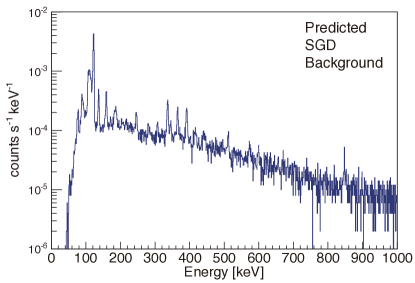
Figure 19: Pre-launch prediction of ASTRO-H SGD background.

6.3 Electron-positron annihilation emission

Scientific Context

An electron-positron pair annihilates into two 511 keV $\gamma$-rays. Since the first detection of the 511 keV line emission from the direction of the Galactic Center (GC) in 1973, the presence has been confirmed by subsequent numerous observations (e.g., Jean et al., 2003). The 511 keV sky map obtained by most recent INTEGRAL/SPI observation revealed that the line emission is quite strong for the Galactic bulge direction centered on the GC and also showed symmetry with the spatial extension of $\sim 8^{\circ}$ (Knodlseder et al., 2005). On the other hand, the emission from the Galactic disk is weak, suggesting that the bulge-to-disk ratio is very large. This is quite different from, for example, the MeV/GeV Galactic diffuse emission revealed by Fermi/LAT. The line flux of the bulge component is measured to be $\sim 1.0\times 10^{-3}$ photons cm^-2 s^-1, but the origin of this strong bulge component is still unclear. On the other hand, positrons responsible for the disk component are thought to be produced by $\beta^{+}$ decay of ⁵⁶Ni, ⁴⁴Ti and ²⁶Al synthesized by SNe.

Although INTEGRAL/SPI has not yet discovered any point sources of the 511 keV line, in the past some papers claimed detection of transient emission of 511 keV line from a point source. Detection and variability of 511 keV line from 1E 1740.7-2942 (known as Great Annihilator) were reported in the literature (Bouchet et al., 1991). Goldwurm et al. (1992) also observed a significant 511 keV feature from Nova Musca. Radioactive decay of ²²Na synthesized during nova explosions should produce a large amount of positrons through the $\beta^{+}$ decay process. Theoretical estimation shows that a strong 511 keV line with flux of $\sim 1.0\times 10^{-4}$ photons cm^-2 s^-1 is emitted when assuming a distance of 10.5 kpc (Suzuki et al., 2010), although this assumed a large amount of ejecta mass of $\sim 10^{-3}M_{\odot}$, which is much larger than $\sim 10^{-5}M_{\odot}$ derived from previous observations and theoretical calculations.

Recent Fermi/LAT detection of MeV/GeV emission from some of novae (e.g., Abdo et al., 2010) provide another channel of producing 511 keV line. In particular, the high-energy $\gamma$-ray emission detected by Fermi/LAT is thought to be produced by the decay of pions produced through $p-p$ interaction. If this is the case, positrons are also generated through decay of $\pi^{+}$. We should keep in mind, however, that the pion decay scenario of MeV/GeV emission from novae is not conclusive, and leptonic origin cannot be ruled out completely.

6.4 Solar Neutrons

The Sun sometimes emits flares whose radiation extends from radio to $\gamma$-ray bands. It is widely accepted that solar flare is caused by magnetic reconnection and the stored magnetic energy is converted into thermal and non-thermal particle velocities (e.g., Tsuneta et al., 1996). Through ground-based and space-borne radio and X-ray observations of solar flares, our knowledge about electron acceleration has been greatly advanced. Ion acceleration, however, can be studied mainly by $\gamma$-ray observation through nuclear de-excitation lines and pion decay emission, but it has been difficult because of the low photon statistics. As a result, comparatively little is known about ion acceleration in solar flares.

Neutrons are also produced during flares through collision of accelerated ions with the solar atmosphere (e.g., Chupp et al., 1982). Hence a measurement of solar neutrons allows us to study ion acceleration in solar flares. Solar neutron measurement has been performed by ground-based telescopes since 1970’s, but as neutrons are significantly attenuated by the Earth’s atmosphere, many assumptions and simulations are needed to infer the neutron spectrum above the atmosphere from observational data obtained by ground-based telescope. Observations in space, of course, can directly and accurately measure the neutron spectrum using far fewer assumptions.

This neutron measurement will be performed with SGD combined with Monte Carlo simulation. Although the SGD is surrounded by a BGO scintillator to reject background, neutrons can penetrate the BGD shield and deposit part of the energy within Si and CdTe detectors. The incoming neutron spectrum will be derived by comparing the observed spectrum as a function of time with Monte Carlo simulation results of different normalizations and power-law indices. The neutron spectrum will provide us with data about accelerated protons above $\sim$30 MeV, while the proton spectrum above $\sim$300 MeV can be estimated from Fermi/LAT observations, if pion decay emission is strong enough. Thus, we can constrain the accelerated proton spectrum above $\sim$30 MeV and obtain information about total number and ratio of accelerated electrons and protons by combining data from other wavelengths.

Table 2: Lines from radioactive isotopes hopefully detected by ASTRO-H/HXI and SGD (taken from Diehl).

Isotope	Life time	Decay chain	Energy [keV]	Source
56Ni	111 d	56Ni$\rightarrow$ 56Co∗	158, 812, 847, 1238	SNe
57Co	390 d	57Co$\rightarrow$ 57Fe∗	122	SNe
44Ti	89 yr	44Ti $\rightarrow$ 44Sc∗ $\rightarrow$ 44Ca∗ + e+	78, 68, 1157	SNe
7Be	77 d	7Be$\rightarrow$ 7Li∗	478	Novae
22Na	3.8 yr	22Na$\rightarrow$ 22Ne∗ + e+	1275	Novae

Appendix A X-ray Spectral Diagnostics

A.1 General Principles

X-ray emission spectra can be created by a range of high-energy processes, and can therefore encode information about those processes. The table below lists the specific diagnostics relevant to the science identified by each ASTRO-H white paper team, but we begin with a brief review of the general possibilities.

Doppler effects: Possibly the simplest diagnostic, using the position and width of an identified emission or absorption line relative to its natural position and width to infer the velocity and turbulence in the emitting or absorbing plasma. The primary challenges are (1) proper identification of the line, (2) ensuring that blending from other nearby lines is not affecting the measurement, and (3) obtaining an accurate laboratory wavelength for the line of interest. Hydrogen-like and helium-like ion lines from $n=2\rightarrow 1$ are well-known from both theory and measurement, but for most other lines in the X-ray the typical accuracy is only at the $50-100$ km s^-1 level (Smith & Brickhouse, 2014).

He-like triplets: The best-known of the X-ray line diagnostics, ratios of the $n=2\rightarrow 1$ lines are functions of temperature, electron density, and ionization state (Porquet et al., 2010). Of course, in reality the system contains many more than three lines; there are four main transitions, and a much larger number of Li-like satellite features that can appear in the triplet ‘bandpass’.

Resonance scattering: Although it behaves in a similar manner as at longer-wavelength bandpasses, obtaining a sufficient column density of ions to observe resonance scattering can be difficult. It has been detected in Fe XVII in elliptical galaxies, as the Fe XVII 15.01Åtransition has a particular large oscillator strength, but the results are confused by ongoing difficulties in understanding the atomic physics of the Fe XVII ion (de Plaa et al., 2012).

Compton shoulders: This feature is a low-energy tail on an emission line generated by Compton scattering of the line-energy photons. Since its spectral characteristics, including its shape, reflect the physical properties of the scattering medium, it potentially provides us with diagnostic tools of the density, electron temperature (or state of electrons), chemical/ion abundances, and geometry. Coupling of all these factors requires both precise modeling of the scattering processes and quantitative evaluation of spectral data.

Absorption edges: Unlike the simple discontinuous jump found in the Henke tables, atomic absorption edges will have detailed structure created by solid state effects (X-ray Absorption Fine Structure, or XAFS), inner-shell excitation, excitation-autoionization effects, and so on. This provides both an opportunity for new diagnostics if the observations, laboratory data, and instrumental calibration are adequate, or it can create confusion requiring the edge to simply be removed from the observations before modeling, as happened for years with the Si edge in many X-ray satellites.

General relativistic redshifts: A strong gravitational field will shift the energy of emission lines; after integrating over the orbit, this has the effect of creating a broad redshifted tail in any emission line, although they are most typically seen in Fe K$\alpha$ lines around AGN or Galactic black holes.

Weak line features from nonthermal emission-dominated sources Although nonthermal sources are often described as featureless power laws, there can exist weak line features due to underlying atomic processes induced by energetic photons, electrons, or ions. The detection of these features by the SXS will bring us new information on astrophysical situations in or around the high-energy sources.

Cyclotron line in strong B-fields: In the presence of a strong magnetic field, electron motion perpendicular to the magnetic field is quantized into corresponding discrete energy levels (so-called ‘Landau levels’). Transitions between the Landau levels leads to absorption-like features in hard X-ray continuum from a magnetized neutron star. These features are also called cyclotron resonance scattering features (CRSFs) since the level transitions usually occur in the context of resonance scattering. Although astrophysical mechanism of generating CRSFs is not well understood, their spectral profiles, which will be obtained with the HXI, will contain important information about the magnetic field, plasma density and temperature, and geometry of the generation site.

K$\beta$ diagnostics, satellite lines: These are both categories of inner-shell transitions that occur in the presence of additional electron (or electrons) in the same shell or an outer shell. This has the effect of moving the transition to somewhat lower energy compared to the same line created without the extra energy. These lines may be weak, but they are useful ionization-state diagnostics since the ratio of the satellite line to the main line strongly depends upon the abundance of the two ions involved.

Non-equilibrium plasma: In practice, electrons in astrophysical collisional plasmas seem to rapidly develop into Boltzmann distributions, although the ionization state of the plasma may take much longer to reach equilibrium. As a result, collisional plasmas will typically either be under- or over-ionized to a degree dependent upon the age and density of the plasma.

Charge exchange: First detected in X-ray observations of comets, CX can be a strong process if the physical precursors of hot ions directly interacting with a neutral plasma can be created. Although a new XSPEC model now exists, the atomic data needed for detailed spectral analysis is still lacking (Smith et al., 2012, 2014).

A.2 Diagnostics by Science Area

A.2.1 Stars

Protostars

Time variation of the Doppler shifts of Fe K lines (6.7 keV, 6.4 keV): The spin and the radius of the central star of a protostar are determined with 6.7 keV line, and the dynamics and the spatial scale of the inner part of the accreting disk are determined with the fluorescent Fe-K line.

Stellar flares

The Doppler shifts of Fe K line (6.7 keV): Dynamic movement of materials during flares will be captured.

Accretion in T Tauri star

The density-sensitive lines: Evidence for accreting plasma will be examined.

Massive stars, colliding wind binaries

Equivalent width and shape of the Compton shoulder of Fe lines: The geometry of wind-wind shock zones will be measured. It means that wind and orbital parameters of CWBs will be obtained.

Diffuse X-rays in star forming regions

Residuals in CCD spectra which could originate from unexpected lines indicating NEI conditions or charge exchange: X-ray emission mechanism(s) of the hot plasma which fills cavities in star forming regions.

Star-planet interaction

Ne line triplet: Plasma density might be determined. Coronal emission might be distinguished from auroral charge-exchange emission, as has been observed in the polar regions of Jupiter.

A.2.2 White Dwarfs

Improved Mass Measurement

G and R ratios of He-like Fe triplet lines: Density and temperature structure of a post-shock region will be! extracted using a help of model calculation based on hydrostatics and plasma cooling functions. Precise determination of temperature structure will lead to WD mass estimation with higher accuracies.

Coronal Disk Measurement

Distorted Fe K emission line shape: Rapid rotation of accretion disk of non-magnetic cataclysmic variables will show red-ward and blue-ward Doppler shift resulting in a distorted emission line profile. By measuring degree of distortion, location of disk coronae which is not well understood in cataclysmic variables will be estimated.

New Mass Measurement

Gravitationally redshifted Fe K fluorescence line: X-ray reflection at the WD surface will produce a redshifted Fe K fluorescence line, and precise measurement of energy shift will provide a new method of WD mass estimation that does not depend on orbital inclination.

A.2.3 X-ray binaries, Magnetars, and Stellar-Mass Black Hole Systems

Two diagnostics were identified for low-mass X-ray binaries, comprised of a compact object such as a neutron star or black hole and a low mass star (e.g. A, F, G, K or M).

Neutron star equation of state

Gravitationally redshifted absorption line: A significant detection of these absorption lines gives a clean measure of M/R.

Wind

Absorption lines in winds: photoionized wind model, geometry, such as the wind in emission from ADC LMXRB

Three were identified for high mass X-ray binaries, systems with a compact object and a massive O or B star.

Wind characteristics

Spectrally and temporally resolve photoionization line profiles particularly of intermediate ionization stages of high-Z elements (Si, S, Fe) and of He-like ions: Determine the wind characteristics of high mass stars, including density temperature, turbulence, radial structure, and asymmetry (e.g., Vela X-1).

Alfven shell

Spin phase resolved fluorescent line profiles: Investigation of kinematics of Alfven shell (e.g., GX 1+4, Her X-1)

Structure of wind

Eclipse mapping of photoionization line strengths with high time resolution, e.g., in Vela X-1: Determine the radial structure of the wind close to high mass stars

Magnetars, neutron stars with extremely large magnetic fields, had two identified diagnostics.

Field strength measurement

Search for proton cyclotron resonance features of magnetars and magnetar-relatives like CCOs.: Direct evidence on the strong magnetic field and interior of magnetars (e.g., 4U 0142+61 and activated sources: see, Tiengo et al., Nature, 2013)

Age estimate

Thermal plasma diagnostics of magnetar-associated supernova remnants: Progenitors of magnetars via the abundance study and magnetar true age via measurements of the Doppler velocity of spectral lines. (e.g., Kes 73 and CTB 109)

Stellar mass black hole systems are a subclass of a X-ray binaries, but have unique science due to the nature of the compact object.

Wind

Detection and characterization of even very weak absorption lines: A strong wind can alter the implied mass accretion rate, which is important to continuum measurements.

Spin

A forest of low-energy atomic emission lines, the Fe line, and the Compton back-scattering hump: Strong constraint or measurement of black hole spin

Accretion Physics

Energy-dependent polarization measurements: To constrain spectral models and reveal the physical state of accreting matter.

A.2.4 Supernova remnants

Kinematics

Doppler-shifted and broadened line structure of each element: Determine the velocity distribution of each element, including expanding velocity, turbulence, anisotropy of ejecta expansion.

Plasma Physics

Forbidden and resonance line ratio of Oxygen in shocks of old SNRs: Determine the influence of charge exchange and resonance scattering effects in the plasma emission.

Abundances

Line broadening in old SNR ejecta: Determine the absolute abundance of old SNR ejecta like Vela shrapnel. In the pure metal case, lines will broaden due to high ion temperature.

Shock Physics

Satellite lines of iron K in over-ionized SNRs: Determine how the shock exchanges thermal energy with interstellar medium.

Pulsar Wind Nebulae

Detecting lines from PWN dominated SNRs: Determine thermal energy and abundance pattern to understand progenitors which made the neutron stars.

Reverse Shock

Measurements of the Fe K$\beta$ line: Diagnostic of the reverse shock in young supernova remnants, such as Tycho

A.2.5 Clusters of galaxies

Cold fronts and mergers

Doppler shift and broadening of the Fe K lines: Measure turbulent and bulk motions in the intracluster medium (ICM) in merging clusters such as Coma and A3667, in order to quantify the spectrum of turbulence and the velocity field across cold fronts. The ultimate goal is to constrain the ICM microphysics.

Gas dynamics, AGN feedback

Doppler shift, broadening and resonant line scattering of the Fe-K lines:Measure turbulent and bulk motions in the brightest cool cores (e.g. Perseus, M87) to constrain AGN feedback

Chemical composition

Emission lines in collisional plasmas: Measure metal abundances of various elements (C, N, O, Ne, Mg, Al, Si, S, Ar, Ca, Cr, Mn, Fe, and Ni) to constrain the metal enrichment histories in galaxies in clusters.

WHIM

Emission line strengths of O: Detect WHIM filaments

Non-thermal pressure and mass

Doppler shift and broadening of Fe K lines: Quantify non-thermal pressure support due to bulk motion and! turbulence, understand cluster growth, energy dissipation in the ICM, cluster masses, and, ultimately, cosmological inferences based on cluster mass estimates

A.2.6 AGNs

Reflection

Shape of the Compton shoulder of fluorescent Fe-K line: Geometry and optical depth of X-ray reflection form gas/dust surrounding the supermassive black hole.

Winds

Doppler shifts and strengths of Fe XXV and Fe XXVI lines: Determine the physics and parameters of the AGN wind, including the total mass in the wind

A.2.7 High-z Universe

High-z chemical evolution

Resonant absorption features in background GRB afterglow or blazar spectra: Chemical evolution in the universe by identifying absorption element and measuring its ionization state due to intergalactic medium (WHIM). The expected temperature, ionization parameter (xi), and redshift are $10^{5Ð6}$ K, $\sim 20$ assuming CXB, and z=1Ð3, respectively.

GRB

Emission Line features of Fe-K and other light elements (Mg, Si, S, Ar, and Ca): Redshift estimation of GRB; chemical evolution study using the GRB associated supernova ejecta; determination of the ejecta mass and velocity.

GRB

Detection and shape of radiative recombination edge: GRB associated SN’s ejecta mass and information on its progenitor by the measured edge energy and the optical depth.

References

- Badnell (1986) Badnell, N. R. 1986, JPhysB, 19, 3827
- Bhardwaj (2007) Bhardwaj, A., et al. 2007, P&SS, 55, 1135
- Cox (1998) Cox, D. P. 1998, LNP, 506, 121
- Cravens (2002) Cravens, T. E. 2002, Science, 296, 1042
- Foster et al. (2014) Foster, A. et al. 2014, in prep.
- Janev & Winter (1985) Janev, R. K., & Winter, H. 1985, Phys. Rep., 117, 265
- Kharchenko & Dalgarno (2001) Kharchenko, V. & Dalgarno, A. 2001, ApJ, 554, L99
- Kharchenko et al. (2003) Kharchenko, V. et al. 2003, ApJL, 585, L73
- Koutroumpa et al. (2006) Koutroumpa, D. et al. 2006, A&A, 460, 289
- Koutroumpa et al. (2009) Koutroumpa, D. et al. 2009, ApJ, 697, 1214
- Smith et al. (2012) Smith, R. K. et al. 2012, Astron. Natch., 333, 301
- Smith et al. (2014) Smith, R. K. et al. 2014, ApJ, 787,77
- Wegmann et al. (1998) Wegmann, R. et al. 1998, P & SS, 46, 603
- Beiersdofer et al. (2003) Beiersdorfer, P., et al. 2003, Science 300, 1558.
- Bhardwaj et al. (2007) Bhardwaj, A., et al. 2007, Planetary and Space Science 55, 1135.
- Branduardi-Raymont et al. (2004) Branduardi-Raymont, G., et al. 2004, Astron. Astrophys. 424, 331.
- Branduardi-Raymont et al. (2007) Branduardi-Raymont, G., et al. 2004, Astron. Astrophys. 463, 761.
- Bodewits et al. (2007) Bodewits, D., et al. 2007, Astron. Astrophys. 469, 1183.
- Carter et al. (2011) Carter, J.A., et al. 2011, Astron. Astrophys. 489, 837.
- Cravens et al. (1997) Cravens, T.E., 1997, Geophys. Res. Lett. 24, 105
- Cravens et al. (2003) Cravens, T.E., 2003, J. Geophys. Res. 108, 1465.
- Dennerl et al. (1997) Dennerl, K., et al. 1997, Science 277, 1625.
- Dennerl et al. (2006) Dennerl, K., et al. 2006, Astron. Astrophys. 451, 709.
- Ezoe et al. (2010a) Ezoe, Y., et al. 2010, Astrophys. J. 709, L178.
- Ezoe et al. (2010b) Ezoe, Y., et al. 2010, Publ. Astron. Soc. Japan, 62, 981.
- Ezoe et al. (2011a) Ezoe, Y., et al. 2011, Adv. Space Research, 47, 411.
- Ezoe et al. (2011b) Ezoe, Y., et al. 2011, Publ. Astron. Soc. Japan, 63, S691.
- Ezoe et al. (2012) Ezoe, Y., et al. 2012, Astron. Nacht., 333, 319.
- Fujimoto et al. (2007) Fujimoto, R., et al. 2007, Publ. Astron. Soc. Japan, 59, S133.
- Gladstone et al. (2002) Gladstone, G.R., et al. 2002, Nature, 1000.
- Ishikawa et al. (2011) Ishikawa, K., et al. 2011, Publ. Astron. Soc. Japan, 63, S702.
- Ishikawa (2013) Ishikawa, K., 2013, private communication (submitted as a Ph.D. thesis at Tokyo Metropolitan University in Japan, 2013 January).
- Lisse et al. (1996) Lisse, C.M., et al. 1996, Science 274, 205.
- Lisse et al. (2003) Lisse, C.M., et al. 2003, Astrophys. J. 635, 1329.
- Porter et al. (2006) Porter, F.S., et al. 2006, Suzaku conf. 2006, Kyoto, Japan.
- Snowden et al. (1994) Snowden, S., et al. 1994, Astrophys. J. 610, 1182.
- Yoshino et al. (2009) Yoshino, T., et al. 2009, Publ. Astron. Soc. Japan, 61, 805.
- Katsuda et al. (2011) Katsuda, S., et al. 2011, ApJ, 730, 24
- Katsuda et al. (2012) Katsuda, S., et al. 2012, ApJ, 756, 49
- Kirshner & Chevalier (1978) Kirshner, R. P., & Chevalier, R. A. 1978, ApJ, 67, 267
- Lallement (2004) Lallement, R. 2004, A&A, 422, 391
- Ohira et al. (2009) Ohira, Y., Terasawa, T., & Takahara, F. 2009, ApJ, 703, L590
- Ohira & Takahara (2010) Ohira, Y., & Takahara, F. 2010, ApJ, 721, L43
- Rasmussen et al. (2001) Rasmussen, A. P., Behar, E., Kahn, S. M., den Herder, J. W., & van der Heyden, K. 2001, A&A, 365, L231
- Wise & Sarazin (1989) Wise, M. W., & Sarazin, C. L. 1989, ApJ, 345, 384
- Liu et al. (2011) Liu, J., Wang, Q.D., Mao, S., et al. 2011, MNRAS, 415, L64
- Liu et al. (2012) Liu, J., Wang, Q.D., Mao, S., et al. 2012, MNRAS, 423, 422
- Ranalli et al. (2008) Ranalli P., Comastri A., Origlia L., Maiolino R., 2008, MNRAS, 386, 1464
- Townsley et al. (2011) Townsley, L.K., Broos, P.S., Chu, Y.-H., Gruendl, R.A., Oey, M.d S., Pittard, J.M. 2011, ApJ, 194, 16
- Tsuru et al. (2007) Tsuru, T.R., et al. 2007, PASJ, 59, 269
- Wang et al. (2001) Wang, Q. D., Immler, S., Walterbos, R., Lauroesch, J. T., Breitschwerdt, D. 2001, ApJ, 555, L99
- Badenes et al. (2008) Badenes, C., et al. 2008, ApJ, 680, L33
- Eriksen et al. (2013) Eriksen, K.A., et al. 2013, submitted to ApJ
- Foster et al. (2012) Foster, A.R., et al. 2012, ApJ, 756, 128
- Gorczyca et al. (2006) Gorczyca, T.W., et al. 2006, ApJ, 638, L121
- Kaastra (1992) Kaastra, J.S. 1992, An X-Ray Spectral Code for Optically Thin Plasmas (Internal SRON-Leiden Report, updated version 2.0)
- Kaastra & Mewe (1993) Kaastra, J.S., & Mewe, R. 1993, A&AS, 97, 443
- Mewe & Schrijver (1985) Mewe, R., & Schrijver J. 1985, Ap&SS, 38, 345
- Mewe et al. (1985) Mewe, R., et al. 1985, A&AS, 62, 197
- Ozawa et al. (2009) Ozawa, M., et al. 2009, ApJ, 706, L71
- Smith et al. (2001) Smith, R.K., et al. 2001, ApJ, 556, L91
- Smith & Hughes (2010) Smith, R.K., & Hughes, J.P. 2010, ApJ, 718, 583
- Yamaguchi et al. (2009) Yamaguchi, H., et al. 2009, ApJ, 705, L6
- Yamaguchi et al. (2014) Yamaguchi, H., et al. 2014, ApJ, 780, 136
- Castor et al. (1975) Castor, J. I., Abbott, D. C., & Klein, R. I. 1975, ApJ, 195, 157
- Detmers et al. (2011) Detmers et al. 2011, A&A, 534, 38
- Evans et al. (2010) Evans et al. 2010, ASPC, 427, 97
- Ferland et al. (1998) Ferland, G. J. et al. 1998, Publications of the Astronomical Society of the Pacific, 110, 761
- Fromerth et al. (2001) Fromerth, M. J., Melia, F., & Leahy, D. A. 2001, ApJ, 547, L129
- Kallman & McCray (1982) Kallman, T. R., & McCray, R. 1982, ApJS, 50, 263
- Tsunemi et al. (2010) Tsunemi, H., et al. 2010, Proc. of SPIE, 7732, 28
- Mitsuda et al. (2010) Mitsuda, K., et al. 2010, Prof. of SPIE, 7732, 29
- Murakami et al. (2001) Murakami, H., Koyama, K., & Maeda, Y. 2001, ApJ, 558, 687
- Odaka (2011) Odaka, H. 2011, Ph. D. thesis, University of Tokyo
- Odaka et al. (2011) Odaka, H., et al. 2011, ApJ, 740, 103
- Leahy & Creighton (1993) Leahy, D. A., & Creighton, J. 1993, MNRAS, 263, 314
- Rybicki & Lightman (1979) Rybicki, G. B., & Lightman, A. P. 1979, Wiley-VCH
- Sim et al. (2008) Sim, S. A. et al. 2008, MNRAS, 388, 611
- Sunyaev & Churazov (1998) Sunyaev, R., & Churazov, E. 1998, MNRAS, 297, 1279
- Sunyaev & Churazov (1996) Sunyaev, R. A., & Churazov, E. M. 1996, Astron. Lett., 22, 648
- Tombesi et al. (2010) Tombesi et al. 2010, A&A, 521, 57
- Watanabe et al. (2003) Watanabe et al. 2003, ApJ, 597, L37
- Watanabe et al. (2006) Watanabe et al. 2006, ApJ, 651, 421
- Ross & Fabian (2005) Ross & Fabian 2005, MNRAS, 358, 211
- Garcia et al. (2010) Garcia, Kallman, & Mushotzky 2011, ApJ, 731, 131
- Yaqoob (2012) Yaqoob 2012, MNRAS, 423, 3360
- Ross et al. (1996) Ross, Fabian, & Brandt 1996, MNRAS, 278, 1082
- Liedahl (2005) Liedahl 2005, AIP Conf. Proc. 774, 99
- Zhuravleva et al. (2010) Zhuravleva et al. 2010, MNRAS, 403, 129
- Jean et al. (2003) Jean et al. 2003, A&A, 407, L55.
- Diehl & Timmes (1998) Diehl & Timmes 1998, PASP, 110, 637.
- Mihara (1995) Mihara 1995, PhD thesis, Univ. of Tokyo.
- Makishima et al. (1999) Makishima et al. 1999, ApJ, 525, 978.
- Nomoto et al. (1984) Nomoto et al. 1984, ApJ, 286, 644.
- Isern et al. (2011) Isern et al. 2011, ATel 3683.
- Maeda et al. (2012) Maeda et al. 2012, ApJ, 760, 54.
- Vink et al. (2001) Vink et al. 2001, ApJ, 560, L79.
- Grebenev et al. (2012) Grebenev et al. 2012, Nature, 490, 373.
- Hernanz & Jose (2006) Hernanz & Jose 2006, New Astronomy Reviews, 50, 504.
- Knodlseder et al. (2005) Knodlseder et al. 2005, A&A, 441, 513.
- Bouchet et al. (1991) Bouchet et al. 1991, ApJ, 383, L45.
- Goldwurm et al. (1992) Goldwurm et al. 1992, ApJ, 389, L79.
- Suzuki et al. (2010) Suzuki et al. 2010, ApJ, 723, L84.
- Abdo et al. (2010) Abdo et al. 2010, Science, 329, 817.
- Tsuneta et al. (1996) Tsuneta et al. 1996, ApJ, 456, 840.
- Chupp et al. (1982) Chupp et al. 1982, ApJ, 263, L95.
- Smith & Brickhouse (2014) Smith, R. K. & Brickhouse, N. S. 2014, Advances in Atomic, Molecular & Optical Physics, in press.
- Porquet et al. (2010) Porquet, D., Dubau, J., & Grosso, N. 2010, Space Science Reviews, 157, 103
- de Plaa et al. (2012) de Plaa, J., Zhuravleva, I., Werner, N., et al. 2012, A&A, 539, A34