On the Weak Convergence and Central Limit Theorem of Blurring and Nonblurring Processes with Application to Robust Location Estimation

Abstract

This article studies the weak convergence and associated Central Limit Theorem for blurring and nonblurring processes. Then, they are applied to the estimation of location parameter. Simulation studies show that the location estimation based on the convergence point of blurring process is more robust and often more efficient than that of nonblurring process.

Keywords: Weak convergence, Central limit theorem, Blurring process, Robust estimation.

1 Introduction

In this article we consider two types of processes arisen from mean-shift algorithms (Fukunaga and Hostetler,, 1975; Cheng,, 1995). Starting with $n$ points $\{x_{i,n}\}_{i=1}^{n}$ as initials, the nonblurring type process is given by

$$x_{i,n}^{[t+1]}=\frac{\int x\,w(x-x_{i,n}^{[t]})dF_{n}(x)}{\int w(x-x_{i,n}^{[t]})dF_{n}(x)}=\sum_{j=1}^{N}\displaystyle\frac{w(x_{j,n}-x_{i,n}^{[t]})}{\sum_{\ell=1}^{N}w(x_{\ell,n}-x_{i,n}^{[t]})}\,x_{j,n},$$ (1)

where $x^{[0]}_{i,n}=x_{i,n}$ and $F_{n}$ is the empirical distribution function based on the initial points $\{x_{i,n}\}_{i=1}^{n}$. This process (1) consists of $n$ simultaneous updating paths, wherein each path starts from one initial. Another type of updating process, called the blurring type, is considered by replacing $F_{n}$ with the iteratively updated empirical distribution $F_{n}^{(t)}$ based on updated points $\{x_{i,n}^{(t)}\}_{i=1}^{n}$, in addition to the above idea of weighted scores for updating:

$$x_{i,n}^{(t+1)}=\frac{\int x\,w(x-x_{i,n}^{(t)})dF_{n}^{(t)}(x)}{\int w(x-x_{i,n}^{(t)})dF_{n}^{(t)}(x)}=\sum_{j=1}^{N}\displaystyle\frac{w(x_{j,n}^{(t)}-x_{i,n}^{(t)})}{\sum_{\ell=1}^{N}w(x_{\ell,n}^{(t)}-x_{i,n}^{(t)})}\,x_{j,n}^{(t)},$$ (2)

where $x^{(0)}_{i,n}=x_{i,n}$. Same as the nonblurring process, the blurring process (2) starts with $n$ initials $\{x_{i,n}\}_{i=1}^{n}$, and then it goes through a simultaneous updating at each iteration. The key difference from the nonblurring process is that, this process (2) takes weighted average according to the updated empirical distribution $F_{n}^{(t)}$, while the nonblurring process takes weighted average with respect to the initial empirical distribution $F_{n}$. That is, at each iteration in the blurring process, not just the weighted centers are updated from $\{x_{i,n}^{(t)}\}_{i=1}^{n}$ to $\{x_{i,n}^{(t+1)}\}_{i=1}^{n}$, the empirical distribution is also updated from $F_{n}^{(t)}$ to $F_{n}^{(t+1)}$.

The blurring process was developed and named SUP (self-updating process in Chen and Shiu, 2007) and was recently applied to cryo-em image clustering (Chen et al., 2014). It is also known as the blurring type mean-shift algorithm (Cheng, 1995; Comaniciu and Meer, 2002). Blurring mean-shift can be viewed as a homogeneous self-updating process. Algorithm convergence and location estimation consistency of the blurring and nonblurring processes were discussed in Cheng, (1995), Comaniciu and Meer, (2002), Li et al., (2007), Chen, (2015), and Ghassabeh, (2015). In this article, we study their weak convergence and associated Central Limit Theorem. Due to the complicated dependent structure of random variables in $\{x_{i,n}^{[t]}\}_{i=1}^{n}$ and $\{x_{i,n}^{(t)}\}_{i=1}^{n}$, the study of their asymptotic behavior becomes challenging.

The convergence point of the blurring or the nonblurring process can be used for location estimation, which is one of the most basic and commonly used tasks in statistical analysis as well as in computer vision. It is well-known that the sample mean is not a robust location estimator and it is sensitive to outliers and data contamination. To reduce the influence from deviant data, there is a wide class of robust M-estimators in statistics literature using weighted scores (Hampel et al., 1986; Huber, 2009; van de Geer, 2000). Consider a weighted score equation for the mean $\mu$:

$$\sum_{i=1}^{n}w(x_{i,n}-\mu)(x_{i,n}-\mu)=0,$$ (3)

where $w(x)$ is a symmetric weight function. The weighted mean that satisfies the estimating equation (3) can be shown to take the following form

$$\mu=\frac{\sum_{i=1}^{n}x_{i,n}w(x_{i,n}-\mu)}{\sum_{i=1}^{n}w(x_{i,n}-\mu)}=\frac{\int xw(x-\mu)dF_{n}(x)}{\int w(x-\mu)dF_{n}(x)}.$$ (4)

This estimator (4) can be obtained by the fixed-point iteration algorithm at convergence, where the iterative update is given by

$$\mu^{[t+1]}=\frac{\int xw(x-\mu^{[t]})dF_{n}(x)}{\int w(x-\mu^{[t]})dF_{n}(x)},\qquad t=0,1,2,\ldots.$$ (5)

with an appropriate starting initial $\mu^{[0]}$. Here, we consider a simple change of the updating process by starting with $n$ data points $\{x_{i,n}\}_{i=1}^{n}$ as initials and by replacing $\mu^{[t]}$ with $x_{i,n}^{[t]}$ in (5). It then leads to the nonblurring process given in (1):

$$x_{i,n}^{[t+1]}=\frac{\int x\,w(x-x_{i,n}^{[t]})dF_{n}(x)}{\int w(x-x_{i,n}^{[t]})dF_{n}(x)}=\sum_{j=1}^{N}\displaystyle\frac{w(x_{j,n}-x_{i,n}^{[t]})}{\sum_{\ell=1}^{N}w(x_{\ell,n}-x_{i,n}^{[t]})}\,x_{j,n}.$$

By replacing $F_{n}$ with $F_{n}^{(t)}$, we have the blurring process given in (2):

$$x_{i,n}^{(t+1)}=\frac{\int x\,w(x-x_{i,n}^{(t)})dF_{n}^{(t)}(x)}{\int w(x-x_{i,n}^{(t)})dF_{n}^{(t)}(x)}=\sum_{j=1}^{N}\displaystyle\frac{w(x_{j,n}^{(t)}-x_{i,n}^{(t)})}{\sum_{\ell=1}^{N}w(x_{\ell,n}^{(t)}-x_{i,n}^{(t)})}\,x_{j,n}^{(t)}.$$

The iterative updating process based on either (1) or (5) has been adopted for robust mean estimation (Field and Smith, 1994; Fujisawa and Eguchi, 2008; Maronna, 1976; Windham, 1995; among others) and robust clustering (Notsu et al., 2014). It is also known as the nonblurring type mean-shift algorithm. On the other hand, robust estimation based on blurring approach is rather rare in the literature. Here we strongly recommend it as an alternative choice. From our simulation studies in Section 3, the blurring type algorithm is often more robust with smaller mean square error. Thus, the blurring type algorithm deserves more attention and further exploration.

The contribution of this article is twofold. First, we derive theoretical properties of the blurring and nonblurring processes including their weak convergence to a Brownian bridge-like process and associated Central Limit Theorem. These theoretical results are presented in Section 2, with all technical proofs being placed in the Appendix. Second, we apply the derived Central Limit Theorem to location estimation. Simulation studies comparing location estimation based on using blurring and nonblurring processes are presented in Section 3. Our simulation results suggest that the blurring type algorithm is often more robust than the existent nonblurring type algorithm for robust M-estimation.

2 Main Results

Let $\{x_{i,n}\in{\mathbb{R}}:i=1,\dots,n\}$, $n\in{\mathbb{N}}$, be a triangular array of random variables. Assume the following conditions.

• The underlying distribution $F$ has a continuous probability density function $f(x)$, which is symmetric about its mean $\mu$.

• The weight function $w(x)$ is a probability density function. It is log-concave and symmetric about 0. (This condition implies that $w(x)>0$ for all $x\in{\mathbb{R}}$ and that $w(x)$ is unimodal and non-constant.)

• For simplicity but without loss of generality, assume $\mu=0$.

2.1 Weak convergence of blurring process

Let $x^{(0)}:=x$ and

$$x^{(t+1)} := \eta^{(t+1)}(x^{(t)})=\eta^{(t+1)}\circ\cdots\circ\eta^{(1)}(x),\quad t=0,1,2,\ldots,$$

where $\eta^{(t+1)}$ is a blurring transformation given by

$$\eta^{(t+1)}(x):=\frac{\int y\cdot w(y-x)dF^{(t)}(y)}{\int w(y-x)dF^{(t)}(y)},$$ (6)

where $\{F^{(t)}\}_{t=0,1,\ldots}$ is the cumulative distribution functions of $X^{(t)}$ with $X^{(0)}\sim F$. Note that the blurring transformation $\eta^{(t+1)}$ shifts $x$ toward a mode by an amount depending on $F^{(t)}$,

$$\frac{\int(y-x)\cdot w(y-x)dF^{(t)}(y)}{\int w(y-x)dF^{(t)}(y)}.$$

Let $\eta_{n}^{(t+1)}$ be the empirical blurring transformation based on $F_{n}^{(t)}$, which is the empirical cumulative distribution of $\{x_{i,n}^{(t)}\}_{i=1}^{n}$. In Theorem 1 below, it is shown $F_{n}^{(t)}(x)\to F^{(t)}(x)$ almost surely for each $x$, as $n\to\infty$. The blurring process, in empirical level and in population level, can be expressed as

$$x_{i,n}^{(t+1)} = \eta_{n}^{(t+1)}(x_{i,n}^{(t)})=\eta_{n}^{(t+1)}\circ\cdots\circ\eta_{n}^{(1)}(x_{i}^{(0)})\quad\mbox{(empirical blurring)},$$

$$x^{(t+1)} = \eta^{(t+1)}(x^{(t)})=\eta^{(t+1)}\circ\cdots\circ\eta^{(1)}(x^{(0)})\quad\mbox{(population blurring)}.$$

At $t=0$, it is known that $F_{n}(x)\to F(x)$ almost surely for each $x$, as $n\to\infty$. Furthermore, by Donsker’s Theorem, the sequence

$$Z_{n}(x):=\sqrt{n}\left(F_{n}(x)-F(x)\right)$$

converges in distribution to a Gaussian process with zero mean and covariance given by

$${\rm Cov}\left(Z_{n}(x),Z_{n}(y)\right)=\min\{F(x),F(y)\}-F(x)F(y).$$

Let this convergence in distribution be denoted by

$$Z_{n}(x):=\sqrt{n}\left(F_{n}(x)-F(x)\right)\rightsquigarrow B(F(x)),$$

where $B$ is the standard Brownian bridge. In this article we establish the weak convergence for the empirical process of cumulative distribution function for each iteration. We will show the weak convergence by mathematical induction. The weak convergence is true at $t=0$ by Donsker’s Theorem. Next, by assuming that $F_{n}^{(s)}(x)\to F^{(s)}(x)$ almost surely and that $\sqrt{n}\left(F_{n}^{(s)}(x)-F^{(s)}(x)\right)\rightsquigarrow B^{(s)}(F(x))$ for some Brownian bridge like process $B^{(s)}$, we show that claimed statements hold for $t=s+1$. Because of the complicated dependent structure in $\{x_{i,n}^{(t)}\}$, the almost sure convergence for $F_{n}^{(t)}(x)$ and the weak convergence for $Z_{n}^{(t)}(x)$ become difficult, where

$$Z_{n}^{(t)}(x):=\sqrt{n}\left(F^{(t)}_{n}(x)-F^{(t)}(x)\right).$$

We first establish the connection between the empirical process of cumulative distribution functions of two consecutive iterations. Then we prove that this connection is a continuous mapping under the Skorokhod topology.

Before establishing the main theorem we derive a few technical lemmas first. Lemma 1, with the proof given in Appendix A.1, shows that $\eta^{{(t)}}$ is a one-to-one transformation, which implies that the data orders do not change during the blurring process at each update. This phenomenon is important when we calculate the empirical cumulative distribution function of the current iteration based on the process of previous iteration.

Lemma 1.

Assume conditions C1-C3. We have $0<\eta^{(t+1)}(a)<\eta^{(t+1)}(b)$ for $0<a<b$.

Next in Lemma 2, we derive the asymptotic behavior of $\eta_{n}^{(t+1)}$, which immediately implies that $F_{n}^{(t+1)}(x)\to F^{(t+1)}(x)$ almost surely.

Lemma 2.

For any $x$, $\lim_{n\to\infty}\eta_{n}^{(t+1)}(x)=\eta^{(t+1)}(x)$ a.s. for $t=0,1,\dots$

The proof is given in Appendix A.2.

To show the weak convergence of $Z_{n}^{(t+1)}(x)$, we need a tighter estimate of $\eta_{n}^{(t+1)}-\eta^{(t+1)}$, which is presented in the following lemma with the proof given in Appendix A.3. While Lemma 2 shows $\eta_{n}^{(t+1)}(x)-\eta^{(t+1)}(x)=o_{p}(1)$, Lemma 3 implies that $\eta_{n}^{(t+1)}-\eta^{(t+1)}(x)=O(1/\sqrt{n})$.

Lemma 3.

For $t=0,1,2,\dots$,

$$\sqrt{n}\left(\eta_{n}^{(t+1)}(x)-\eta^{(t+1)}(x)\right)=\frac{\int\left(y-\eta_{n}^{(t+1)}(x)\right)w(y-x)\,dZ_{n}^{(t)}(y)}{\int w(y-x)dF^{(t)}(y)}.$$ (7)

Let $\xi^{(t)}$ and $\xi_{n}^{(t)}$ be the inverse function of $\eta^{(t)}$ and $\eta_{n}^{(t)}$, respectively. Then, we have

$$F^{(t+1)}(x)=P\left\{X^{(t+1)}\leq x\right\}=P\left\{\eta^{(t+1)}(X^{(t)})\leq x\right\}=F^{(t)}({\xi^{(t+1)}}(x)).$$

Using this formula and the Taylor expansion, we establish the connection between $Z_{n}^{(t+1)}(x)$ and $Z_{n}^{(t)}(x)$. The result is presented in the following lemma with the proof given in Appendix A.4.

Lemma 4.

The process $Z_{n}^{(t+1)}(x)$ can be expressed as a function of the previous process $Z_{n}^{(t)}(x)$ up to an additive $o_{p}(1)$-term. Precisely,

$$Z_{n}^{(t+1)}(x)=\int_{y}\left\{K^{(t+1)}(x,y)+o_{p}(1)\right\}dZ_{n}^{(t)}(y),$$ (8)

where

$$K^{(t+1)}(x,y)=-\frac{f^{(t+1)}(x)\cdot(y-x)w(y-\xi^{(t+1)}(x))}{{\int w\left(y-\xi^{(t+1)}(x)\right)dF^{(t)}(y)}}+1_{\{y\leq\xi^{(t+1)}(x)\}}.$$ (9)

With the assumption of the weak convergence of $Z_{n}^{(t)}(x)$ to a Brownian bridge-like process, the variance of $\int_{y}o_{p}(1)dZ_{n}^{(t)}(y)$ will also be $o_{p}(1)$.

Lemma 5 below states that the mapping (8), ignoring $o_{p}(1)$, is continuous. The continuity is stated in Lemma 5 with the proof given in Appendix A.5.

Lemma 5.

Let ${\cal D}={\cal D}[0,1]$ be the space of real-valued functions on $[0,1]$ that are right-continuous and have left-hand limits. Define ${\cal L}^{(t+1)}$ as a mapping from ${\cal D}$ to ${\cal D}$, such that

$$({\cal L}^{(t+1)}W)(u)=\int_{v=0}^{1}K^{(t+1)}\left(F^{-(t)}(u),F^{-(t)}(v)\right)\,dW(v)\quad\forall W\in{\cal D},$$ (10)

where $F^{-(t)}(u)$ denotes the inverse function of $F^{(t)}(x)$. Then, ${\cal L}^{(t+1)}$ is continuous under the Skorokhod topology.

Let $B_{n}^{(t)}(u):=Z_{n}^{(t)}(F^{-(t)}(u))$. Then $B_{n}^{(t)}(u)\in{\cal D}$, and

$$B_{n}^{(t+1)}(u)=\int_{v=0}^{1}\left\{K^{(t+1)}(F^{-(t)}(u),F^{-(t)}(v))+o_{p}(1)\right\}dB_{n}^{(t)}(v).$$

Lemma 5 shows that the mapping is asymptotically continuous. Therefore, $B_{n}^{(t+1)}$ has the same weak convergence property as $B_{n}^{(t)}$. The result is summarized in Theorem 1.

Theorem 1.

Assume conditions C1-C3. We have

1. For each $x$, $F_{n}^{(t)}(x)\to F^{(t)}(x)$ almost surely, as $n\to\infty$;

2. $\sqrt{n}\left(F_{n}^{(t)}(x)-F^{(t)}(x)\right)\rightsquigarrow B^{(t)}(F^{(t)}(x))$, where $B^{(0)}$ is the standard Brownian bridge on $[0,1]$, $B^{(t)}(u)=\int_{v=0}^{1}H^{(t)}(u,v)dB^{(0)}(v)$, $H^{(1)}(u,z):=K^{(1)}(F^{-1}(u),F^{-1}(z))$, and

   $$H^{(t+1)}(u,z):=\int_{v=0}^{1}K^{(t+1)}(F^{-(t)}(u),F^{-(t)}(v))\frac{\partial H^{(t)}(v,z)}{\partial v}\,dv.$$

Proof for Theorem 1 is in Appendix A.6.

Corollary 1.

$B^{(t)}(0)=B^{(t)}(1)=0$ and ${{\rm Cov}\left\{B^{(t)}(u),B^{(t)}(v)\right\}=\int_{0}^{1}H^{(t)}(u,z)H^{(t)}(v,z)dz}$.

2.2 Weak convergence of nonblurring process

In the nonblurring process we use almost the same notation as in the blurring process except for the superscript $[t]$. A similar result for the nonblurring process is stated in the following theorem with its proof given in Appendix A.7.

Theorem 2.

Assume conditions C1-C3. We have

1. For each $x$, $F_{n}^{[t]}(x)\to F^{[t]}(x)$ almost surely, as $n\to\infty$;

2. $\sqrt{n}\left(F_{n}^{[t]}(x)-F^{[t]}(x)\right)\rightsquigarrow B^{[t]}(F(x))$, where $B^{(0)}$ is the standard Brownian bridge on $[0,1]$, $B^{[t]}(u)=\int_{0}^{1}H^{[t]}(u,v)dB^{(0)}(v)$ with

   $$H^{[1]}(u,v)~{}~{}\, := K^{[1]}(F^{-1}(u),F^{-1}(v))+1_{\left\{\eta^{[1]}(F^{-1}(v))\leq F^{-1}(u)\right\}}\,,$$

   $$H^{[t+1]}(u,v) := K^{[t+1]}(F^{-1}(u)),F^{-1}(v))+H^{[t]}\left(F(\xi^{[t+1]}(F^{-1}(u))),F(\xi^{[t+1]}(F^{-1}(v)))\right).$$

2.3 Central Limit Theorem

Apply the weak convergence, we can have the Central Limit Theorem for the sample mean of updated data. The result on the blurring case is presented below with its proof given in Appendix A.8

Theorem 3.

Let $S_{n}^{(t+1)}:=\frac{1}{\sqrt{n}}\sum_{i=1}^{n}x_{i,n}^{(t+1)}$. We have

$$S_{n}^{(t+1)}\rightsquigarrow\int\int\left(\frac{w(x-y)x}{\rho^{(t)}(y)}+\frac{w(y-x)y}{\rho^{(t)}(x)}\right)dF^{(t)}(x)dB^{(t)}(F^{(t)}(y)),$$

where $\rho^{(t)}(y)=E_{X\sim F^{(t)}}\left(w(X-y)\right)$.

From Theorem 1,

$$B^{(t)}(u)=\int_{v=0}^{1}H^{(t)}(u,v)dB^{(0)}(v).$$

Take the derivative, we have

$$dB^{(t)}(u)=\int_{v=0}^{1}\frac{\partial H^{(t)}(u,v)}{\partial u}dB^{(0)}(v)du.$$

Now substitute $u=F^{(t)}(y)$ in the above equation. We have

$$dB^{(t)}(F^{(t)}(y))=\int_{v=0}^{1}\frac{\partial H^{(t)}(u,v)}{\partial u}\Big{|}_{u=F^{(t)}(y)}dB^{(0)}(v)dF^{(t)}(y).$$

Therefore

$$\int\int\left(\frac{w(x-y)x}{\rho^{(t)}(y)}+\frac{w(y-x)y}{\rho^{(t)}(x)}\right)dF^{(t)}(x)dB^{(t)}(F^{(t)}(y))$$

$$= \int\int\left(\frac{w(x-y)x}{\rho^{(t)}(y)}+\frac{w(y-x)y}{\rho^{(t)}(x)}\right)dF^{(t)}(x)\int_{v=0}^{1}\frac{\partial H^{(t)}(u,v)}{\partial u}\Big{|}_{u=F^{(t)}(y)}dB^{(0)}(v)dF^{(t)}(y).$$

$$= \int_{v=0}^{1}\left[\int\int\left(\frac{w(x-y)x}{\rho^{(t)}(y)}+\frac{w(y-x)y}{\rho^{(t)}(x)}\right)\frac{\partial H^{(t)}(u,v)}{\partial u}\Big{|}_{u=F^{(t)}(y)}dF^{(t)}(x)dF^{(t)}(y)\right]dB^{(0)}(v)$$

This distribution has mean 0, and variance

$$\int_{v=0}^{1}\left[\int\int\left(\frac{w(x-y)x}{\rho^{(t)}(y)}+\frac{w(y-x)y}{\rho^{(t)}(x)}\right)\frac{\partial H^{(t)}(u,v)}{\partial u}\Big{|}_{u=F^{(t)}(y)}dF^{(t)}(x)dF^{(t)}(y)\right]^{2}dv.$$

The Central Limiting Theorem for the nonblurring case is similar, and the proof is almost identical and thus is omitted. The update of the nonblurring process is a weighted average over the original data and the weights depend on the updated data at the previous iteration.

Theorem 4.

Let $S_{n}^{[t+1]}:=\frac{1}{\sqrt{n}}\sum_{i=1}^{n}x_{i,n}^{[t+1]}$. We have

$$S_{n}^{[t+1]} \rightsquigarrow \int\int\frac{w(x-y)x}{\rho(y)}dF(x)dB^{[t]}(F^{[t]}(y))+\int\int\frac{w(y-x)y}{\rho(x)}dF^{[t]}(x)dB^{(0)}(F(y)),$$

where $\rho(y)=E_{X\sim F}\left(w(X-y)\right)$.

3 Application to robust location estimation with simulation studies

The convergence point with either the blurring or the nonblurring process is a reasonable robust estimation of the location parameter. The consistency of the nonblurring process is proved in Cheng, (1995), and that of the blurring process is proved in Chen, (2015). With the Central Limit Theorem provided in the previous section, it is of our interest to compare the efficiency of both processes. Theoretical comparison of asymptotic variance is quite difficult even for the simplest case that both the sampling distribution and the weight function are normal. In below we will first explain the rationale behind the phenomenon that blurring is more robust and often more efficient than nonblurring. Then, we will show by simulation studies the behavior of asymptotic normality and the mean square error comparison for both processes.

Without the update of empirical distribution i.e., by keeping the initial empirical distribution $F_{n}$ throughout all iterations in the nonblurring process, the effective weights in (1) are approaching

$$\frac{w(x-\mu^{[\tau]})}{\int w(x-\mu^{[\tau]})dF_{n}(x)},$$

where $\tau$ is the last iteration step at convergence. With the update of empirical distribution in the blurring process, the effective weights in (2) are getting more and more close to uniform. Since the weighted average is taken with respect to newly updated centers, each of which is a weighted average of previous updated centers, the contribution of each original data point to the final estimation is relatively uniform for the blurring process, while the contribution of each data point in the nonblurring process is governed by $w(x)$. It is known that the sample mean, which corresponds to a uniform weight, is the uniformly minimum variance unbiased estimator for many distributions including normal distribution. While both blurring and nonblurring estimators are robust by reducing the contribution of outliers or data points in heavy tails, the blurring estimator, which takes a relatively uniformly weight, is expected to be more efficient than the nonblurring estimator on processing the relatively reliable part of information. Our simulation results presented in Section 3.2 also support this thinking.

3.1 Asymptotic normality

In this simulation study, we compare the asymptotic normality of blurring and nonblurring processes. In theory all points should converge to a common point (Chen,, 2015) if the weight function has unbounded support. However, in empirical data simulation (in particular, the case of Student-$t$ distribution presented below) some points far away from the main data cloud may fail to move to the location where most points have converged to, due to the precision in computer and the stopping criterion in the data implementation. Therefore, we take the median value at the stopping of the updating process. Precisely, let $\mu^{(\tau)}_{n,m}:={\rm median}\{x_{i,n,m}^{(\tau)},\,i=1,2,\dots,n\}$ and $\mu^{[\tau]}_{n,m}:={\rm median}\{x_{i,n,m}^{[\tau]},\,i=1,2,\dots,n\}$, where $\tau$ is the number of iteration steps at convergence for the $m^{\rm th}$ replicate run for $m=1,2,\dots,M$. Here we take $M=500$. Data are generated from $N(0,1)$, Uniform$(0,1)$, and Student-$t$ with 3 degrees of freedom, where the sample size $n$ is set to 400. Two kinds of weight functions, normal and double exponential, are used. In Figures 1 and 2, QQ-plots for $\{\mu^{(\tau)}_{n,m}:m=1,2,\dots,M\}$ and $\{\mu^{[\tau]}_{n,m}:m=1,2,\dots,M\}$ are presented for two kinds of weight functions. We also include QQ-plots using sample means (for normal and uniform distributions) and sample medians (for Student-$t$ distribution) as a reference asymptotic behavior. For the Student-$t$, it requires a much larger $n$ for the sample means to behave like a normal. Thus, we used sample medians, which require less larger $n$. It can be seen that both $\{\mu^{(\tau)}_{n,m}\}_{m=1}^{M}$ and $\{\mu^{[\tau]}_{n,m}\}_{m=1}^{M}$ well follow a normal distribution. Furthermore, the slopes in nonblurring QQ-plots are a bit steeper than those in the blurring ones. It indicates that the convergence point of nonblurring process tends to have a larger variance.

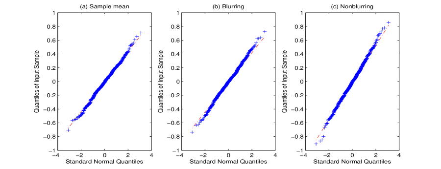
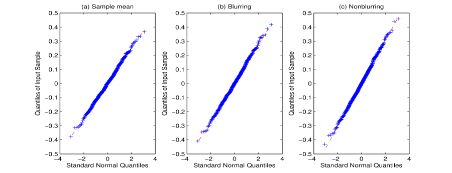
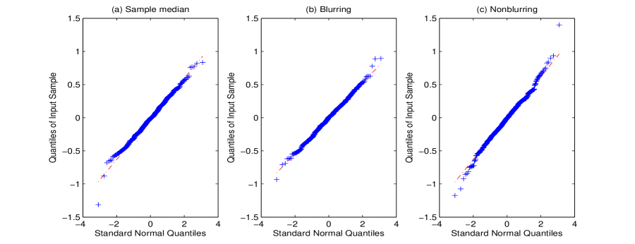
Figure 1: QQ-plots. Sampling distributions are normal (top row), uniform (middle row) and Student-$t$ (bottom row). Weight function is normal.

    
 
    

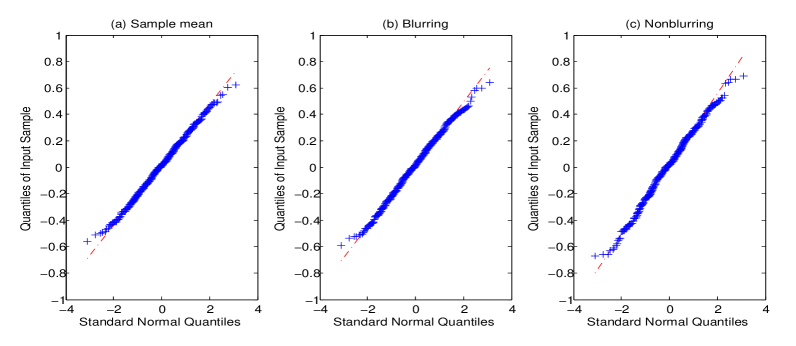
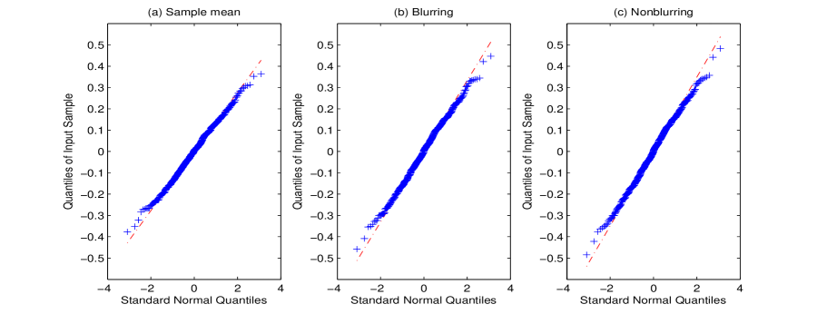
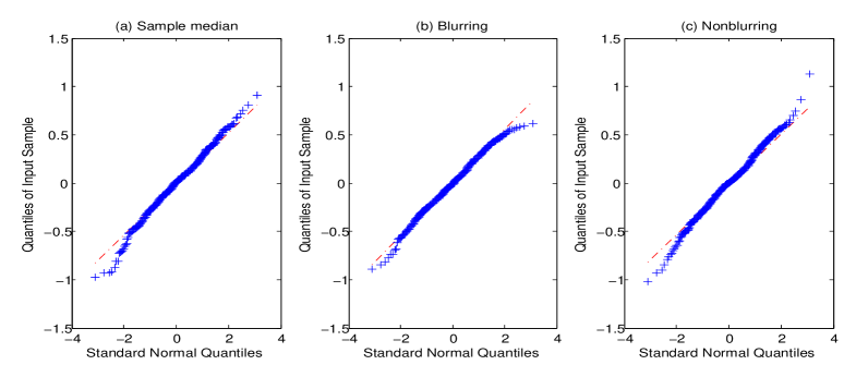
Figure 2: QQ-plots. Sampling distributions are normal (top row), uniform (middle row) and Student-$t$ (bottom row). Weight function is double exponential.

3.2 Mean square error comparison

In this simulation study, we compare mean square errors (MSE) of $\{\mu^{(\tau)}_{n,m}\}_{m=1}^{M}$ and $\{\mu^{[\tau]}_{n,m}\}_{m=1}^{M}$, which are obtained from blurring and nonblurring processes, respectively. Three types of data distributions are used, $N(0,1)$, ${\rm Uniform}(-1,1)$ and Student-$t$ with 3, 5 and 10 degrees of freedom. Normal and double exponential weight functions are adopted. Sample size is set to $n=10^{2},12^{2},14^{2},\ldots,30^{2}$. The mean square errors are calculated based on $M=10,000$ multiple trials.

Plots of $n\times$MSE against the square root of sample size $\sqrt{n}$ are presented. We also include MSE of sample means and sample medians for comparison. Sample mean is the UMVUE for estimating the normal mean. From Figure 3 (a) and (b), we can see that the sample mean has the smallest MSEs for data generated from normal. Estimates by the nonblurring process have larger MSEs compared to those by blurring process. We have experimented with various parameter values of normal and double exponential as the weight functions. All the results show that

$$\mbox{sample mean MSE $<$ blurring estimate MSE $<$ nonblurring estimate MSE $<$ sample median MSE}.$$

Similar phenomena can be observed for data generated from the uniform $(0,1)$ distribution, which are depicted in Figure 3 (c) and (d).

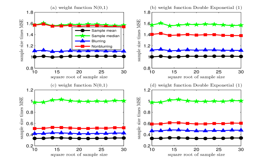
Figure 3: MSE comparison. (a) and (b): sampling distribution is normal $N(0,1)$; (c) and (d): sampling distribution is uniform $(0,1)$

For heavy-tailed distributions such as Student-$t$ distributions, the performance of blurring estimate, nonblurring estimate, sample mean and sample median for estimating location parameter depends on the weight function. Figure 4 presents the results by normal weight functions with various parameter values, when the sampling distribution is Student-$t$ with 3 degrees of freedom. As expected, the sample median is better than the sample mean in estimating the location parameter of Student-$t$ distribution. In general, blurring estimates have smaller or competitive MSEs than those by nonblurring estimates. They produce a bit larger MSEs than the nonblurring ones only when an effectively flat weight function, such as $N(0,\sigma^{2})$ with $\sigma^{2}=4$ and $9$, is used. Similar phenomena for double exponential weight functions on Student-$t$ can be observed in Figure 5.

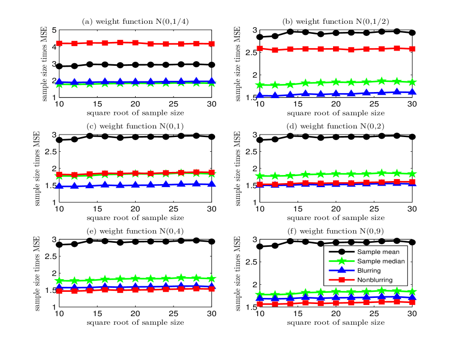
Figure 4: MSE comparison for sampling distribution Student-$t$ with 3 degrees of freedom and normal weight function.

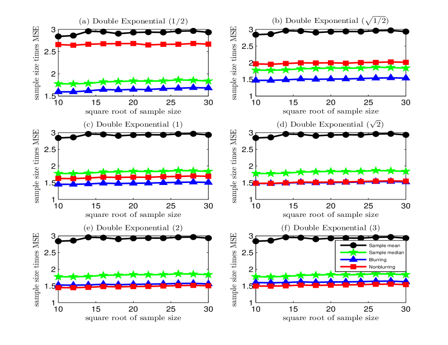
Figure 5: MSE comparison for sampling distribution Student-$t$ with 3 degrees of freedom and double exponential weight function.

To further compare MSEs of all estimates, in Figure 6 we summarize the MSE results with sample size $n=900$ on cases from Figures 4 and 5. From Figure 6, the best-performance weight functions for blurring estimates are $N(0,1)$ and double exponential with mean parameter equal to 1. The best-performance weight functions for nonblurring estimates are $N(0,4)$ and double exponential with mean 2. All the MSE values are very close in these 4 best-performance cases. While the nonblurring estimation produces much larger MSEs for peaked weight functions, the performance of blurring estimation is still competitive with nonblurring for relatively flat weight function. Therefore, blurring is viewed as a more robust estimator for Student-$t$. We have also extended the experiment to Student-$t$ distributions with 5 and 10 degrees of freedom. The results are presented in Figures 7-12. They all support that the blurring estimates are more robust in the sense of smaller or competitive MSEs. The theoretic aspects behind these findings would be worthy of further exploration.

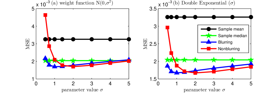
Figure 6: Summary of MSE comparison for sampling distribution Student-$t$ with 3 degrees of freedom.

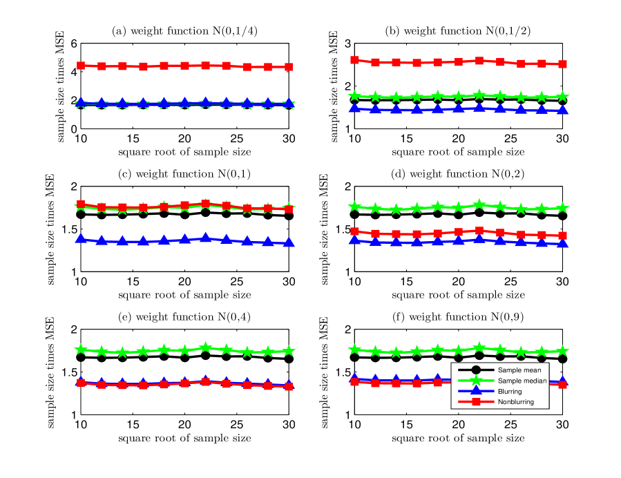
Figure 7: MSE comparison for sampling distribution Student-$t$ with 5 degrees of freedom and normal weight function.

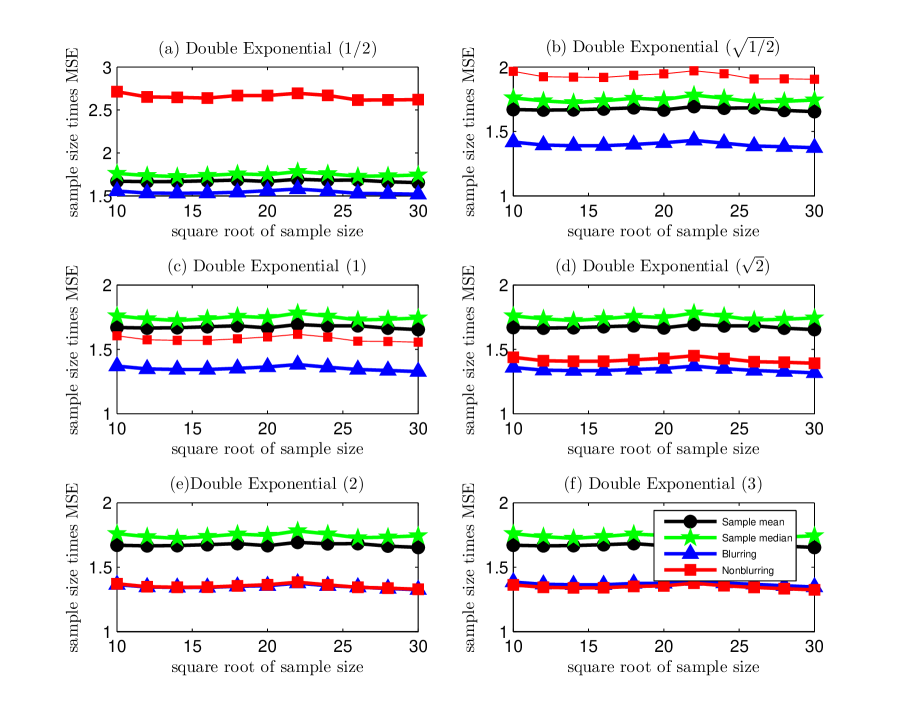
Figure 8: MSE comparison for sampling distribution Student-$t$ with 5 degrees of freedom and double exponential weight function.

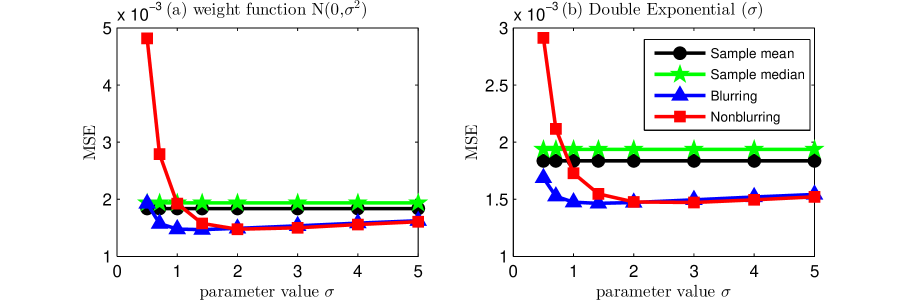
Figure 9: Summary of MSE comparison for sampling distribution Student-$t$ with 5 degrees of freedom.

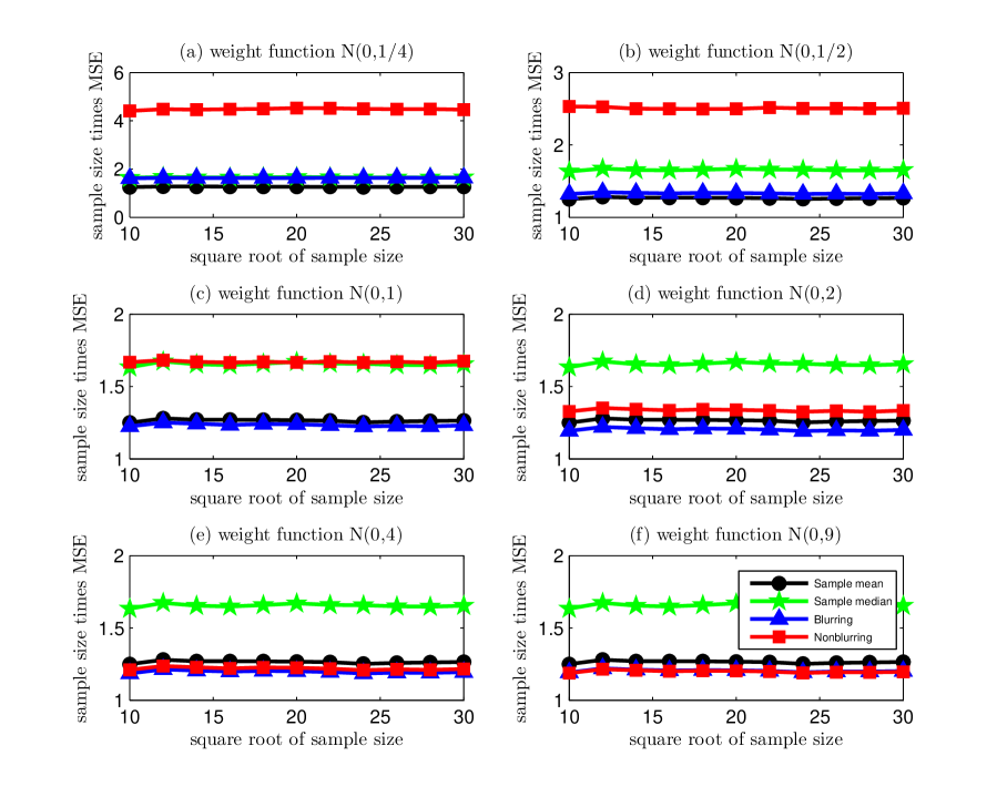
Figure 10: MSE comparison for sampling distribution Student-$t$ with 10 degrees of freedom and normal weight function.

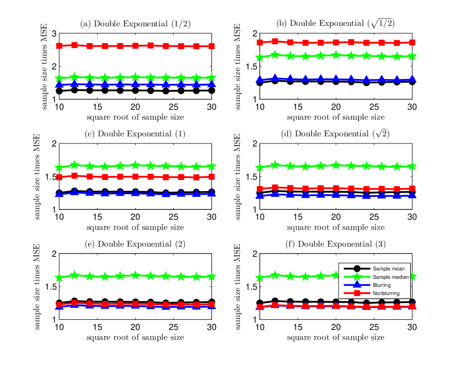
Figure 11: MSE comparison for sampling distribution Student-$t$ with 10 degrees of freedom and double exponential weight function.

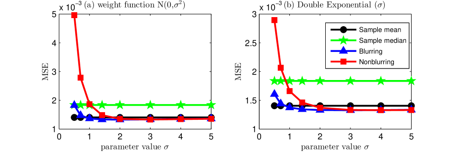
Figure 12: Summary of MSE comparison for sampling distribution Student-$t$ with 10 degrees of freedom.

4 Conclusion

In this article, we have established the weak convergence and associated Central Limit Theorem for the blurring and nonblurring processes. Convergence points from both types of processes can be used for robust M-estimation of location. In our simulation study, it shows that the blurring type has a smaller mean square error than the nonblurring type if a weight function is reasonably chosen. The nonblurring type estimation is often adopted in robust statistics literature. Our simulation results suggest that we shall consider the blurring type algorithm as an alternative choice to the existent nonblurring type algorithm for robust M-estimation.

Appendix A Appendix

Except for Lemma 3 with a direct proof, we will show the rest lemmas and Theorem 1 by mathematical induction. For each individual lemma or theorem, we will first show that it is valid for $t=0$. Next by assuming the validity of Lemmas 1-5 as well as Theorem 1 for $t$ and the validity of preceding lemmas for $t+1$, we will establish the claim of the current target lemma. For instance, say, the current target lemma that we want to prove is Lemma 4. We first show that Lemma 4 is valid for $t=0$. Next, by assuming that Lemmas 1-5 and Theorem 1 hold for $t$ and further assuming that Lemmas 1-3 hold for $t+1$, we will establish the claim of Lemma 4 for $t+1$.

A.1 Proof of Lemma 1

Proof.

We will prove that for $0<a<b$,

$$\eta^{(1)}(a)=\frac{\int_{-\infty}^{\infty}xw(x-a)f(x)dx}{\int_{-\infty}^{\infty}w(x-a)f(x)dx}<\frac{\int_{-\infty}^{\infty}xw(x-b)f(x)dx}{\int_{-\infty}^{\infty}w(x-b)f(x)dx}=\eta^{(1)}(b).$$

for any symmetric probability density function $f$. The proof for $\eta^{(t+1)}(a)<\eta^{(t+1)}(b)$ is identically the same. We first consider the case that $\eta^{(1)}(a)\leq\frac{a+b}{2}$. From

$$\frac{\int_{-\infty}^{\infty}xw(x-a)f(x)dx}{\int_{-\infty}^{\infty}w(x-a)f(x)dx}=\eta^{(1)}(a),$$

we have

$$\int_{-\infty}^{\eta^{(1)}(a)}(\eta^{(1)}(a)-x)w(x-a)f(x)dx=\int_{\eta^{(1)}(a)}^{\infty}(x-\eta^{(1)}(a))w(x-a)f(x)dx.$$

Since $w$ is log-concave, for any $d>0$, $\log(w(x+d))-\log(w(x))$ is non-increasing for all $x$. Therefore

$$\frac{w(x-a)}{w(x-b)}\geq\frac{w(\eta^{(1)}(a)-a)}{w(\eta^{(1)}(a)-b)}\equiv\gamma\quad\quad\forall x<\eta^{(1)}(a).$$

and

$$\frac{w(x-a)}{w(x-b)}\leq\gamma\quad\quad\forall x>\eta^{(1)}(a).$$

Then

$$\int_{-\infty}^{\eta^{(1)}(a)}(\eta^{(1)}(a)-x)w(x-a)f(x)dx\geq\gamma\int_{-\infty}^{\eta^{(1)}(a)}(\eta^{(1)}(a)-x)w(x-b)f(x)dx.$$ (11)

Similar, we have

$$\int_{\eta^{(1)}(a)}^{\infty}(x-\eta^{(1)}(a))w(x-a)f(x)dx<\gamma\int_{\eta^{(1)}(a)}^{\infty}(x-\eta^{(1)}(a))w(x-b)f(x)dx.$$ (12)

Note that $\gamma\geq 1$ since $\eta^{(1)}(a)<\frac{a+b}{2}$ . Since $w$ is non-constant, there exists $x>\frac{a+b}{2}$, such that $\frac{w(x-a)}{w(x-b)}<1\leq\gamma$. Therefore the inequality in (12) is strictly less. Combining (11) and (12), we have

$$\int_{-\infty}^{\infty}(x-\eta^{(1)}(a))w(x-b)f(x)dx$$

$$= \int_{-\infty}^{\eta^{(1)}(a)}(x-\eta^{(1)}(a))w(x-b)f(x)dx+\int_{\eta^{(1)}(a)}^{\infty}(x-\eta^{(1)}(a))w(x-b)f(x)dx$$

$$> \frac{1}{\gamma}\int_{-\infty}^{\eta^{(1)}(a)}(x-\eta^{(1)}(a))w(x-a)f(x)dx+\frac{1}{\gamma}\int_{\eta^{(1)}(a)}^{\infty}(x-\eta^{(1)}(a))w(x-a)f(x)dx$$

$$= \frac{1}{\gamma}\int_{-\infty}^{\infty}(x-\eta^{(1)}(a))w(x-a)f(x)dx=0$$

Therefore

$$\eta^{(1)}(b)-\eta^{(1)}(a)=\frac{\int_{-\infty}^{\infty}(x-\eta^{(1)}(a))w(x-b)f(x)dx}{\int_{-\infty}^{\infty}w(x-b)f(x)dx}>0.$$

For the case that $\eta^{(1)}(a)>\frac{a+b}{2}$, the proof is almost the same. Now

$$\frac{w(x-b)}{w(x-a)}\geq\frac{w(\eta^{(1)}(a)-b)}{w(\eta^{(1)}(a)-a)}\equiv\theta\quad\quad\forall x>\eta^{(1)}(a).$$

Then we have

$$\int_{\eta^{(1)}(a)}^{\infty}(x-\eta^{(1)}(a))w(x-b)f(x)dx\geq\theta\int_{\eta^{(1)}(a)}^{\infty}(x-\eta^{(1)}(a))w(x-a)f(x)dx$$

and

$$\int_{-\infty}^{\eta^{(1)}(a)}(\eta^{(1)}(a)-x)w(x-b)f(x)dx<\theta\int_{-\infty}^{\eta^{(1)}(a)}(\eta^{(1)}(a)-x)w(x-a)f(x)dx.$$

Combining both will again lead to $\eta^{(1)}(b)-\eta^{(1)}(a)>0$.

∎

A.2 Proof of Lemma 2

Proof.

Similar to Lemma 1, we will prove this lemma for $\eta_{n}^{(1)}$. The proof for $\eta_{n}^{(t+1)}$ is identically the same. By definition, we have

$$\eta_{n}^{(1)}(x)=\frac{\int yw(y-x)dF_{n}(y)}{\int w(y-x)dF_{n}(y)}.$$ (13)

Since $w$ is finite integrable, $(y-x)w(y-x)$ is bounded. Then, there exists a constant $M<\infty$ such that

$$|yw(y-x)|\leq|(y-x)w(y-x)|+|xw(0)|\leq M+|x|w(0).$$

From the weak convergence of $F_{n}$, we have

$$\lim_{n\to\infty}\int yw(y-x)dF_{n}(y) = \int yw(y-x)dF(y)\quad\mbox{ a.s. }$$ (14)

$$\lim_{n\to\infty}\int w(y-x)dF_{n}(y)~{}~{} = \int w(y-x)dF(y)\quad\mbox{ a.s. }$$ (15)

Also note that, for a fixed $x$

$$\int w(y-x)dF(y)>\int_{0}^{x}w(y-x)dF(y)>(F(x)-1/2)\times w(-x)$$

is bounded away from $0$. Thus, from (13), (14) and (15),

$$\lim_{n\to\infty}\eta_{n}^{(1)}(x)=\eta^{(1)}(x)\quad\mbox{ a.s. }$$

∎

A.3 Proof of Lemma 3

Proof.

Let

$$\alpha_{n} = \int yw(y-x)dF_{n}^{(t)}(y),\;\;\alpha\,~{}=\,\int yw(y-x)dF^{(t)}(y),$$

$$\beta_{n} = \int w(y-x)dF_{n}^{(t)}(y),\;\;~{}\,\beta~{}\,=\,~{}\int w(y-x)dF^{(t)}(y).$$

Then,

$$\sqrt{n}\left(\eta_{n}^{(t+1)}(x)-\eta^{(t+1)}(x)\right)=\sqrt{n}\left(\frac{\alpha_{n}}{\beta_{n}}-\frac{\alpha}{\beta}\right)$$

$$= \sqrt{n}\left(\frac{\alpha_{n}}{\beta}-\frac{\alpha}{\beta}+\frac{\alpha_{n}}{\beta_{n}}-\frac{\alpha_{n}}{\beta}\right)=\sqrt{n}\left(\frac{\alpha_{n}-\alpha}{\beta}-\frac{\alpha_{n}(\beta_{n}-\beta))}{\beta_{n}\beta}\right)$$

$$= \frac{1}{\beta}\int yw(y-x)d\sqrt{n}\left(F^{(t)}_{n}(y)-F^{(t)}(y)\right)$$

$$-\frac{\alpha_{n}}{\beta_{n}\beta}\int w(y-x)d\sqrt{n}\left(F^{(t)}_{n}(y)-F^{(t)}(y)\right)$$

$$= \frac{\int(y-\eta_{n}^{(t+1)}(x))w(y-x)d\sqrt{n}\left(F^{(t)}_{n}(y)-F^{(t)}(y)\right)}{\int w(y-x)dF^{(t)}(y)}.$$

∎

A.4 Proof of Lemma 4

Proof.

$$Z_{n}^{(t+1)}(x)=\sqrt{n}\left(F_{n}^{(t+1)}(x)-F^{(t+1)}(x)\right)$$ (16)

$$= \sqrt{n}\left(F_{n}^{(t)}(\xi_{n}^{(t+1)}(x))-F^{(t)}(\xi^{(t+1)}(x)\right)$$

$$= \sqrt{n}\left(F_{n}^{(t)}(\xi_{n}^{(t+1)}(x))-F_{n}^{(t)}(\xi^{(t+1)}(x)\right)+\sqrt{n}\left(F_{n}^{(t)}(\xi^{(t+1)}(x))-F^{(t)}(\xi^{(t+1)}(x)\right)$$

$$= \sqrt{n}\left(F_{n}^{(t)}(\xi_{n}^{(t+1)}(x))-F_{n}^{(t)}(\xi^{(t+1)}(x)\right)+\int 1_{\{y\leq\xi^{(t+1)}(x)\}}\,dZ_{n}^{(t)}(x).$$

For the first term, we need to to calculate $\xi_{n}^{(t+1)}(x)-\xi^{(t+1)}(x)$. Since $\eta_{n}^{(t+1)}(x)$ converges to $\eta^{(t+1)}(x)$ almost surely, the inverse function $\xi_{n}^{(t+1)}(x)$ also converges to $\xi^{(t+1)}(x)$ almost surely. Note that $x=\eta^{(t+1)}(\xi^{(t+1)}(x))$. Expanding $\xi_{n}^{(t+1)}(\cdot)$ at $\eta_{n}^{(t+1)}(\xi^{(t+1)}(x))$, we have

$$\xi_{n}^{(t+1)}(x)-\xi^{(t+1)}(x)$$

$$= \xi_{n}^{(t+1)}\left(\eta_{n}^{(t+1)}(\xi^{(t+1)}(x))\right)-\frac{d\xi_{n}^{(t+1)}(u)}{du}\Big{|}_{u=\tau_{n}}\cdot\left(\eta_{n}^{(t+1)}(\xi^{(t+1)}(x))-x\right)-\xi^{(t+1)}(x)$$

$$= -\frac{d\xi_{n}^{(t+1)}(u)}{du}\Big{|}_{u=\tau_{n}}\cdot\left(\eta_{n}^{(t+1)}(\xi^{(t+1)}(x))-\eta^{(t+1)}(\xi^{(t+1)}(x))\right)$$

$$= -\left(\frac{d\xi^{(t+1)}(u)}{du}\Big{|}_{u=x}+o_{p}(1)\right)\cdot\left(\eta_{n}^{(t+1)}(\xi^{(t+1)}(x))-\eta^{(t+1)}(\xi^{(t+1)}(x))\right),$$

where $\tau_{n}$ is some number between $x$ and $\eta_{n}^{(t+1)}(\xi^{(t+1)}(x))$. Since $\eta_{n}^{(t+1)}\to\eta^{(t+1)}$ a.s., $\eta_{n}^{(t+1)}(\xi^{(t+1)}(x))\to x$ a.s. Therefore, $\tau_{n}\to x$ a.s. Then the first term in (16) can be calculated as follows.

$$\sqrt{n}\left(F_{n}^{(t)}(\xi_{n}^{(t+1)}(x))-F_{n}^{(t)}(\xi^{(t+1)}(x)\right)$$ (17)

$$= \frac{dF_{n}^{(t)}(\xi)}{d\xi}\Big{|}_{\xi=c_{n}}\times\sqrt{n}\,\left(\xi_{n}^{(t+1)}(x)-\xi^{(t+1)}(x)\right)$$

$$= \left\{\frac{dF^{(t)}(\xi)}{d\xi}\Big{|}_{\xi=\xi^{(t+1)}(x)}+o_{p}(1)\right\}\times\bigg{\{}-\left(\frac{d\xi^{(t+1)}(u)}{du}\Big{|}_{u=x}+o_{p}(1)\right)$$

$$\times\sqrt{n}\left(\eta_{n}^{(t+1)}(\xi^{(t+1)}(x))-\eta^{(t+1)}(\xi^{(t+1)}(x))\right)\bigg{\}}$$

$$= -\left(\frac{dF^{(t+1)}(u)}{du}\Big{|}_{u=x}+o_{p}(1)\right)\times\sqrt{n}\left(\eta_{n}^{(t+1)}(\xi^{(t+1)}(x))-\eta^{(t+1)}(\xi^{(t+1)}(x))\right)$$

$$= -f^{(t+1)}(x)\times\sqrt{n}\left(\eta_{n}^{(t+1)}(\xi^{(t+1)}(x))-\eta^{(t+1)}(\xi^{(t+1)}(x))\right)+o_{p}(1),$$

where $c_{n}$ is some number between $\xi_{n}^{(t+1)}(x)$ and $\xi^{(t+1)}(x)$. Apply (7) in Lemma 3 to (17), and then this lemma can be established. ∎

A.5 Proof of Lemma 5

Proof.

Let $\Lambda$ denote the class of strictly increasing continuous mappings from $[0,1]$ onto itself. For $\lambda\in\Lambda$, define

$$\|\lambda\|:=\sup_{0\leq u\leq v\leq 1}\left|\log\left(\frac{\lambda(t)-\lambda(u)}{v-u}\right)\right|.$$

The metric of $\cal D$ is defined by (see, e.g., Billingsley 1968)

$$d(f_{1},f_{2})=\inf_{\lambda}\,\max\left\{\|\lambda\|,\sup_{0\leq u\leq 1}\left|f_{1}(u)-f_{2}(\lambda(u))\right|\right\},~{}~{}f_{1},f_{2}\in{\cal D}.$$

The topology generated by this metric is called the Skorokhod topology. For $d(f_{1},f_{2})<\delta$, there exists $\widetilde{\lambda}$ such that

$$\max\{\|\widetilde{\lambda}\|,\sup_{0\leq u\leq 1}|f_{1}(u)-f_{2}(\widetilde{\lambda}(u))|\}<\delta.$$

This implies that

$$\|\widetilde{\lambda}\|<\delta\qquad{\rm and}\qquad\sup_{0\leq u\leq 1}|f_{1}(u)-f_{2}(\widetilde{\lambda}(u))|<\delta.$$

Then, we have

$$\left|({\cal L}^{(t+1)}f_{1})(u)-({\cal L}^{(t+1)}f_{2})(\widetilde{\lambda}(u))\right|$$

$$= \left|\int_{v=0}^{1}K^{(t+1)}(F^{-(t)}(u),F^{-(t)}(v))d\left(f_{1}(v)-f_{2}(\widetilde{\lambda}(v))\right)\right|$$

$$\leq \delta\int_{v=0}^{1}\left|K^{(t+1)}(F^{-(t)}(u),F^{-(t)}(v))\right|dv.$$

Plugging in defining expression for $K^{(t+1)}$, we have

$$\int_{v=0}^{1}\left|K^{(t+1)}(F^{-(t)}(u),F^{-(t)}(v))\right|dv$$

$$= \int_{y=-\infty}^{\infty}\left|K^{(t+1)}(x,y)\right|dF^{(t)}(y)\quad\quad\quad\quad\quad(x=F^{-(t)}(u),y=F^{-(t)}(v))$$

$$= \int_{y=-\infty}^{\infty}\left|-\frac{f^{(t+1)}(x)\cdot(y-x)w(y-\xi^{(t+1)}(x))}{{\int w\left(y-\xi^{(t+1)}(x)\right)dF^{(t)}(y)}}+1_{\{y\leq\xi^{(t+1)}(x)\}}\right|dF^{(t)}(y)$$

$$\leq \int_{y=-\infty}^{\infty}\left|\frac{f^{(t+1)}(x)\cdot|y+x|\cdot w(y-\xi^{(t+1)}(x))}{{\int w\left(y-\xi^{(t+1)}(x)\right)dF^{(t)}(y)}}\right|dF^{(t)}(y)+1.$$

Note that

$$\int_{y=-\infty}^{\infty}\left|\frac{f^{(t+1)}(x)\cdot xw(y-\xi^{(t+1)}(x))}{{\int w\left(y-\xi^{(t+1)}(x)\right)dF^{(t)}(y)}}\right|dF^{(t)}(y)=f^{(t+1)}(x)|x|,$$

and that

$$\int_{y=-\infty}^{\infty}\left|\frac{yw(y-\xi^{(t+1)}(x))}{\int w\left(y-\xi^{(t+1)}(x)\right)dF^{(t)}(y)}\right|dF^{(t)}(y)$$

$$= \int_{y=-|x|}^{|x|}\left|\frac{yw(y-\xi^{(t+1)}(x))}{{\int w\left(y-\xi^{(t+1)}(x)\right)dF^{(t)}(y)}}\right|dF^{(t)}(y)+\int_{y>|x|}\left|\frac{yw(y-\xi^{(t+1)}(x))}{{\int w\left(y-\xi^{(t+1)}(x)\right)dF^{(t)}(y)}}\right|dF^{(t)}(y)$$

$$\leq \int_{y=-\infty}^{\infty}\left|\frac{xw(y-\xi^{(t+1)}(x))}{{\int w\left(y-\xi^{(t+1)}(x)\right)dF^{(t)}(y)}}\right|dF^{(t)}(y)+\int_{y>|x|}\left|\frac{yw(y-\xi^{(t+1)}(x))}{{\int w\left(y-\xi^{(t+1)}(x)\right)dF^{(t)}(y)}}\right|dF^{(t)}(y)$$

$$= |x|+R^{(t)}(x),$$

where

$$R^{(t)}(x):=\int_{y>|x|}\left|\frac{yw(y-\xi^{(t+1)}(x))}{{\int w\left(y-\xi^{(t+1)}(x)\right)dF^{(t)}(y)}}\right|dF^{(t)}(y)\to 0\quad\mbox{ as }|x|\to\infty.$$

Therefore, for $d(f_{1},f_{2})<\delta$ and $f_{1},f_{2}\in{\cal D}[0,1]$, we have

$$d({\cal L}f_{1},{\cal L}f_{2}) \leq \max\left\{\|\widetilde{\lambda}\|,\sup_{0\leq u\leq 1}|({\cal L}f_{1})(u)-({\cal L}f_{2})(\widetilde{\lambda}(u))|\right\}$$

$$< \delta\left\{f^{(t+1)}(x)(2|x|+R^{(t)}(x))+1\right\},~{}~{}{\rm where~{}}x=F^{-(t)}(u).$$

Hence, ${\cal L}$ is continuous. ∎

A.6 Proof of Theorem 1

Proof.

We will prove this theorem by mathematical induction. For $t=0$, statements (i) and (ii) are well-known results as almost sure convergence of empirical CDF and Donsker’s Theorem, respectively. (See, e.g., Dudley, 1999.) Assume statements (i) and (ii) hold for $t=s$. Then, statement (i) with $t=s+1$ is an immediate result of Lemma 2. It is now left to show statement (ii) with $t=s+1$ to complete the proof by mathematical induction.

Recall that $B_{n}^{(s)}(u)=Z_{n}^{(s)}(F^{-(s)}(u))$. By Lemma 5,

$$B^{(s+1)}(u)=\int_{v=0}^{1}K^{(s+1)}(F^{-(s)}(u),F^{-(s)}(v))dB^{(s)}(v).$$

By assumption $B^{(s)}(u)=\int H^{(s)}(u,z)dB^{(0)}(z)$, then

$$dB^{(s)}(u)=\int\frac{\partial H^{(s)}(u,z)}{\partial u}\,dB^{(0)}(z)\,du.$$

Therefore,

$$B^{(s+1)}(u) = \int_{v=0}^{1}K^{(s+1)}(F^{-(s)}(u),F^{-(s)}(v))dB^{(s)}(v)$$

$$= \int_{v=0}^{1}\int_{z=0}^{1}K^{(s+1)}(F^{-(s)}(u),F^{-(s)}(v))\frac{\partial H^{(s)}(v,z)}{\partial v}\,dB^{(0)}(z)\,dv$$

$$= \int_{z=0}^{1}\int_{v=0}^{1}K^{(s+1)}(F^{-(s)}(u),F^{-(s)}(v))\frac{\partial H^{(s)}(v,z)}{\partial v}\,dv\,dB^{(0)}(z)$$

$$= \int_{z=0}^{1}H^{(s+1)}(u,z)dB^{(0)}(z),$$

where $H^{(1)}(u,z):=K^{(1)}(F^{-1}(u),F^{-1}(z))$ and

$$H^{(s+1)}(u,z):=\int_{v=0}^{1}K^{(s+1)}(F^{-(s)}(u),F^{-(s)}(v))\frac{\partial H^{(s)}(v,z)}{\partial v}\,dv.$$

By mathematical induction, we have shown the almost sure convergence of $F_{n}^{(t)}$ and the weak convergence of $\sqrt{n}\left(F_{n}^{(t)}(x)-F^{(t)}(x)\right)$. ∎

A.7 Proof of Theorem 2

Proof.

We will use similar mathematical induction arguments to prove the weak convergence for the nonblurring case. For $t=1$, nonblurring and blurring process are identically the same. Therefore the statements hold for $t=1$. Assume that they hold for $t=s$, we will prove that they hold for $t=s+1$. Since

$$\eta^{[s]}(x)=\frac{\int y\cdot w(y-x)dF(y)}{\int w(y-x)dF(y)},$$

$\eta^{[s]}(x)$’s are the same for all $t$, i.e. $\eta^{[1]}(x)=\eta^{[2]}(x)=\cdots$. With the same arguments for blurring process, we have

$$\lim_{n\to\infty}\eta_{n}^{[s+1]}(x)=\eta^{[s+1]}(x),$$

and

$$\sqrt{n}\left(\eta_{n}^{[s+1]}(x)-\eta^{[s+1]}(x)\right)=\frac{\int(y-\eta_{n}^{[s+1]}(x))w(y-x)d\sqrt{n}\left(F_{n}(y)-F(y)\right)}{\int w(y-x)dF(y)}.$$

Then by similar arguments,

$$\sqrt{n}\left(F_{n}^{[s+1]}(x)-F^{[s+1]}(x)\right)$$ (18)

$$= \sqrt{n}\left(F_{n}^{[s]}(\xi_{n}^{[s+1]}(x))-F_{n}^{[s]}(\xi^{[s+1]}(x)\right)+\sqrt{n}\left(F_{n}^{[s]}(\xi^{[s+1]}(x))-F^{[s]}(\xi^{[s+1]}(x)\right)$$

$$= \left(\frac{dF^{[s]}(\xi)}{d\xi}\Big{|}_{\xi=\xi^{[s+1]}(x)}+o_{p}(1)\right)\cdot\left(-\frac{d\xi^{[s+1]}(u)}{du}\Big{|}_{u=x}+o_{p}(1)\right)$$

$$\times\sqrt{n}\left(\eta_{n}^{[s+1]}(\xi^{[s+1]}(x))-\eta^{[s+1]}(\xi^{[s+1]}(x))\right)$$

$$+\sqrt{n}\left(F_{n}^{[s]}(\xi^{[s+1]}(x))-F^{[s]}(\xi^{[s+1]}(x)\right)$$

$$= \int_{y}(K^{[s+1]}(x,y)+o_{p}(1))\,d\sqrt{n}\left(F_{n}(y)-F(y)\right)$$

$$+\sqrt{n}\left(F_{n}^{[s]}(\xi^{[s+1]}(x))-F^{[s]}(\xi^{[s+1]}(x)\right),$$

where

$$K^{[s+1]}(x,y)=-\frac{f^{[s+1]}(x)\cdot(y-x)w(y-\eta^{-[s+1]}(x))}{{\int w(y-\eta^{-[s+1]}(x))dF(y)}}.$$

For $t=1$,

$$\sqrt{n}\left(F_{n}^{[1]}(x)-F^{[1]}(x)\right)$$

$$= \int_{y}(K^{[1]}(x,y)+o_{p}(1))\,d\sqrt{n}\left(F_{n}(y)-F(y)\right)+\sqrt{n}\left(F_{n}^{[0]}(\xi^{[1]}(x))-F^{[0]}(\xi^{[1]}(x)\right)$$

$$= \int_{y}(K^{[1]}(x,y)+1_{\{y\leq\xi^{[1]}(x)\}}+o_{p}(1))\,d\sqrt{n}\left(F_{n}(y)-F(y)\right)$$

$$= \int_{y}(K^{[1]}(x,y)+1_{\{\eta^{[1]}(y)\leq x\}}+o_{p}(1))\,d\sqrt{n}\left(F_{n}(y)-F(y)\right).$$

Let $H^{[1]}(u,v)=K^{[1]}(F^{-1}(u),F^{-1}(v))+1_{\{\eta^{[1]}(F^{-1}(v))\leq F^{-1}(u)\}}$. By mathematical induction assumption of the statement at $t=s$, we have

$$\sqrt{n}\left(F_{n}^{[s]}(\xi^{[s+1]}(x))-F^{[s]}(\xi^{[s+1]}(y))\right)$$

$$= \int_{y}\left\{H^{[s]}\left(F(\xi^{[s+1]}(x)),F(\xi^{[s+1]}(y))\right)+o_{p}(1)\right\}d\sqrt{n}\left(F_{n}(y)-F(y)\right),$$

where $H^{[t]}$, $t=1,2,\dots$, is defined iteratively via (19). Take this into (18), it becomes

$$\sqrt{n}\left(F_{n}^{[s+1]}(x)-F^{[s+1]}(x)\right)$$

$$= \int_{y}\left\{K^{[s+1]}(x,y)+H^{[s]}\left(F(\xi^{[s+1]}(x)),F(\xi^{[s+1]}(y))\right)+o_{p}(1)\right\}d\sqrt{n}\left(F_{n}(y)-F(y)\right)$$

$$= \int_{y}(H^{[s+1]}(F(x),F(y))+o_{p}(1))d\sqrt{n}\left(F_{n}(y)-F(y)\right),$$

where

$$H^{[s+1]}(u,v):=K^{[s+1]}(F^{-1}(u)),F^{-1}(v))+H^{[s]}\left(F(\xi^{[s+1]}(F^{-1}(u))),F(\xi^{[s+1]}(F^{-1}(v)))\right).$$ (19)

Then by similar arguments as in the blurring case, we have

$$\sqrt{n}\left(F_{n}^{[s+1]}(x)-F^{[s+1]}(x)\right)\rightsquigarrow B^{[s+1]}(F(x)),$$

where

$$B^{[s+1]}(u)=\int_{v=0}^{1}H^{[s+1]}(u,v)dB^{[0]}(v).$$

∎

A.8 Proof of Theorem 3

Proof.

From

$$\rho^{(t)}(x_{i,n}^{(t)})=\frac{1}{n}\sum_{j=1}^{n}w(x_{j,n}^{(t)}-x_{i,n}^{(t)})+o_{p}(1),$$

then

$$\frac{\sum_{j=1}^{n}\frac{1}{n}w(x_{j,n}^{(t)}-x_{i,n}^{(t)})x_{j,n}^{(t)}}{\sum_{j=1}^{n}\frac{1}{n}w(x_{j,n}^{(t)}-x_{i,n}^{(t)})}-\frac{\sum_{j=1}^{n}\frac{1}{n}w(x_{j,n}^{(t)}-x_{i,n}^{(t)})x_{j,n}^{(t)}}{\rho^{(t)}(x_{i,n}^{(t)})}$$

$$= \frac{\sum_{j=1}^{n}\frac{1}{n}w(x_{j,n}^{(t)}-x_{i,n}^{(t)})x_{j,n}^{(t)}}{\sum_{j=1}^{n}\frac{1}{n}w(x_{j,n}^{(t)}-x_{i,n}^{(t)})}\cdot\frac{\rho^{(t)}(x_{i,n}^{(t)})-\sum_{j=1}^{n}\frac{1}{n}w(x_{j,n}^{(t)}-x_{i,n}^{(t)})}{\rho^{(t)}(x_{i,n}^{(t)})}$$

$$= o_{p}(1),$$

since $\frac{\sum_{j=1}^{n}w(x_{j,n}^{(t)}-x_{i,n}^{(t)})x_{j,n}^{(t)}}{\sum_{j=1}^{n}w(x_{j,n}^{(t)}-x_{i,n}^{(t)})}$ is bounded. Therefore

$$S_{n}^{(t+1)} = \frac{1}{\sqrt{n}}\sum_{i=1}^{n}x_{i,n}^{(t+1)}=\frac{1}{\sqrt{n}}\sum_{i=1}^{n}\frac{\sum_{j=1}^{n}w(x_{j,n}^{(t)}-x_{i,n}^{(t)})x_{j,n}^{(t)}}{\sum_{j=1}^{n}w(x_{j,n}^{(t)}-x_{i,n}^{(t)})}$$ (20)

$$= \frac{1}{n\sqrt{n}}\sum_{i,j=1}^{n}\frac{w(x_{j,n}^{(t)}-x_{i,n}^{(t)})x_{j,n}^{(t)}}{\rho^{(t)}(x_{i,n}^{(t)})}+o_{p}(1)$$

$$= \sqrt{n}\int\int\frac{w(x-y)x}{\rho^{(t)}(y)}dF_{n}^{(t)}(x)dF_{n}^{(t)}(y)+o_{p}(1).$$

Next, we have

$$\sqrt{n}\left(\int\int\frac{w(x-y)x}{\rho^{(t)}(y)}dF_{n}^{(t)}(x)dF_{n}^{(t)}(y)-\int\int\frac{w(x-y)x}{\rho^{(t)}(y)}dF^{(t)}(x)dF^{(t)}(y)\right)$$ (21)

$$= \sqrt{n}\left(\int\int\frac{w(x-y)x}{\rho^{(t)}(y)}dF_{n}^{(t)}(x)dF_{n}^{(t)}(y)-\int\int\frac{w(x-y)x}{\rho^{(t)}(y)}dF_{n}^{(t)}(x)dF^{(t)}(y)\right)$$

$$+\sqrt{n}\left(\int\int\frac{w(x-y)x}{\rho^{(t)}(y)}dF_{n}^{(t)}(x)dF^{(t)}(y)-\int\int\frac{w(x-y)x}{\rho^{(t)}(y)}dF^{(t)}(x)dF^{(t)}(y)\right).$$

By Fubini theorem, since the integral of the absolute value is finite, we can change the order.

$$(\ref{eq:Sn2}) = \sqrt{n}\left(\int\int\frac{w(x-y)x}{\rho^{(t)}(y)}dF_{n}^{(t)}(x)dF_{n}^{(t)}(y)-\int\int\frac{w(x-y)x}{\rho^{(t)}(y)}dF_{n}^{(t)}(x)dF^{(t)}(y)\right)$$

$$+\sqrt{n}\left(\int\int\frac{w(x-y)x}{\rho^{(t)}(y)}dF^{(t)}(y)dF_{n}^{(t)}(x)-\int\int\frac{w(x-y)x}{\rho^{(t)}(y)}dF^{(t)}(y)dF^{(t)}(x)\right)$$

$$= \int\int\frac{w(x-y)x}{\rho^{(t)}(y)}dF_{n}^{(t)}(x)d\sqrt{n}(F_{n}^{(t)}(y)-F^{(t)}(y))$$

$$+\int\int\frac{w(x-y)x}{\rho^{(t)}(y)}dF^{(t)}(y)d\sqrt{n}(F_{n}^{(t)}(x)-F^{(t)}(x))$$

$$\to \int\left(\int(\frac{w(x-y)x}{\rho^{(t)}(y)}+\frac{w(y-x)y}{\rho^{(t)}(x)})dF^{(t)}(x)\right)dB^{(t)}(F^{(t)}(y)).$$

Since

$$\int\int\frac{w(x-y)x}{\rho^{(t)}(y)}dF^{(t)}(x)dF^{(t)}(y)=0,$$

then

$$S_{n}^{(t+1)} = S_{n}^{(t+1)}-\sqrt{n}\int\int\frac{w(x-y)x}{\rho^{(t)}(y)}dF^{(t)}(x)dF^{(t)}(y)$$

$$\to \int\int\left(\frac{w(x-y)x}{\rho^{(t)}(y)}+\frac{w(y-x)y}{\rho^{(t)}(x)}\right)dF^{(t)}(x)dB^{(t)}(F^{(t)}(y)).$$

∎

References

- Billingsley, (1968) Billingsley, P. (1968). Convergence of Probability Measures, New York, Wiley.
- Basu et al., (1998) Basu, A., Harris, I. R., Hjort, N. L., and Jones, M. C. (1998). Robust and efficient estimation by minimising a density power divergence. Biometrika, 85(3):549–559.
- Chen, (2015) Chen, T.-L. (2015). On the convergence and consistency of the blurring mean-shift process. Annals of the Institute of Statistical Mathematics, 67(1):157-176.
- (4) Chen, T.L., Hsieh, D.N., Hung, H., Tu, I.P., Wu, P.S., Wu, Y.M., Chang, W. and Huang, S.Y. (2014). -SUP: a clustering algorithm for cryo-electron microscopy images of asymmetric particles. Annals of Applied Statistics, 8(1):259–285.
- Chen and Shiu, (2007) Chen, T.-L. and Shiu, S.-Y. (2007). A clustering algorithm by self-updating process. JSM Proceedings, Statistical Computing Section, Salt Lake City, Utah; American Statistical Association, pp:2034–2038.
- Cheng, (1995) Cheng, Y. (1995). Mean shift, mode seeking, and clustering. IEEE Transactions on Pattern Analysis and Machine Intelligence, 17:790–799.
- Comaniciu and Meer, (2002) Comaniciu, D. and Meer, P. (2002). Mean shift: a robust approach toward feature space analysis. IEEE Transactions on Pattern Analysis and Machine Intelligence, 24(5):603-619.
- (8) Dudley, R.M. (1999). Uniform Central Limit Theorems. Cambridge University Press.
- Field and Smith, (1994) Field, C. and Smith, B. (1994). Robust estimation: a weighted maximum likelihood approach. International Statistical Review, 62(3):405–424.
- Fujisawa and Eguchi, (2008) Fujisawa, H. and Eguchi, S. (2008). Robust parameter estimation with a small bias against heavy contamination. Journal of Multivariate Analysis, 99:2053–2081.
- Fukunaga and Hostetler, (1975) Fukunaga, K. and Hosterler, L. D. (1975). The estimation of the gradient of a density function, with applications in pattern recognition. IEEE Trans. Inform. Theory, 21(1):32–40.
- Ghassabeh, (2015) Ghassabeh, Y.A. (2015). A sufficient condition for the convergence of the mean shift algorithm with Gaussian kernel. Journal of Multivariate Analysis, 135:1-10.
- (13) Hampel, F.R., Ronchetti, E.M., Rousseeuw, P.J. and Stahel, W.A. (1986). Robust Statistics: The Approach Based on Influence Functions, New York, Wiley.
- (14) Huber, P. (2009). Robust Statistics, 2nd ed. John Wiley & Sons Inc.
- Li et al., (2007) Li, X., Hu, Z. and Wu, W. (2007). A note on the convergence of the mean shift. Pattern Recognition, 40(6), 1756–1762.
- (16) Maronna, R.A. (1976). Robust M-estimators of multivariate location and scatter. Annals of Statistics, 4(1):51–67.
- (17) Notsu, A., Komori, O. and Eguchi, S. (2014). Spontaneous clustering via minimum gamma-divergence. Neural Computation, 26:421–448.
- (18) van de Geer, S.A. (2000). Empirical Processes in M-estimation: Applications of Empirical Process Theory, Cambridge Series in Statistical and Probabilistic Mathematics, Cambridge University Press.
- Windham, (1995) Windham, M. P. (1995). Robustifying model fitting. Journal of the Royal Statistical Society, Series B-Methodology, 57(3):599–609.