Measurement of Holmium Rydberg series through MOT depletion spectroscopy

Abstract

We report measurements of the absolute excitation frequencies of ¹⁶⁵Ho $4f^{11}6sns$ and $4f^{11}6snd$ odd-parity Rydberg series. The states are detected through depletion of a magneto-optical trap via a two-photon excitation scheme. Measurements of 162 Rydberg levels in the range $n=40-101$ yield quantum defects well described by the Rydberg-Ritz formula. We observe a strong perturbation in the $ns$ series around $n=51$ due to an unidentified interloper at 48515.47(4) cm^-1. From the series convergence, we determine the first ionization potential $E_{\mathrm{IP}}=48565.939(4)$ cm^-1, which is three orders of magnitude more accurate than previous work. This work represents the first time such spectroscopy has been done in Holmium and is an important step towards using Ho atoms for collective encoding of a quantum register.

I Introduction

Rydberg atoms have been studied extensively, yielding important information about atomic structure and ionization thresholds Gallagher (1988); Aymar et al. (1996). Rydberg atoms are attracting intense current interest in the area of quantum information processing due to their strong dipole-dipole interactions Saffman et al. (2010). Rydberg dipole blockade provides a strong, switchable interaction between neutral atoms, allowing for the creation of quantum gates and entanglementLukin et al. (2001). Two-qubit gates have so far been demonstrated in the alkali atoms rubidium Isenhower et al. (2010); Wilk et al. (2010) and cesiumMaller et al. (2014). There is further interest in using the Rydberg blockade in ensembles of atoms to create a collectively encoded quantum register Lukin et al. (2001); Brion et al. (2007). Collective encoding is most beneficial in atoms with a large number of ground hyperfine states Saffman and Mølmer (2008). The stable atom with the largest number of hyperfine ground states is holmium. Its nuclear spin is $I=7/2$ and the electronic angular momentum of the ground state is $J=15/2$, providing 128 hyperfine ground states with total angular momentum $F=4-11$. The large angular momentum arises due to the open $4f$-shell in the ground state electronic configuration. As with other rare-earth elements, this open shell structure results in an extremely complex energy spectrum that is challenging to reproduce theoretically due to strong relativistic effects and configuration interactions Biémont (2005). For Rydberg atom quantum information processing, knowledge of the Rydberg levels is important for accurate prediction of the dipole-dipole interaction strengths and sensitivity to external fields.

Studies of the Rydberg spectra of neutral rare earth elements have been limited to date, with initial measurements of the ionization potentials for the full range of lanthanides Worden et al. (1978) and actinides Erdmann et al. (1998) and energy resolved Rydberg states for La Xue et al. (1997), Eu Nakhate et al. (2000), Dy Xu et al. (1992), Lu Ogawa and Kujirai (1999), Gd Miyabe et al. (1998), Sm Jayasekharan et al. (2000), Th Vidolova-Angelova et al. (1984), Ce Vidolova-Angelova et al. (1997), Yb Camus et al. (1980), Ac Roßnagel et al. (2012), Pu Worden et al. (1993) and U Solarz et al. (1976). In this paper we present the first high resolution spectroscopy of the $4f^{11}6sns$ and $4f^{11}6snd$ odd-parity Rydberg states of Ho in the range $n=40-101$ using depletion measurements on a magneto optical trap (MOT). The resulting spectra are used to extract accurate values for the first ionization potential and quantum defects for the series, in addition to revealing a strong perturbation around $51s$ which is analyzed in the framework of multi-channel quantum defect theory (MQDT). Additionally, we observe a previously unpublished repumper transition from a metastable state giving significant enhancement in the MOT atom number. These measurements provide important information about the fundamental atomic structure of the open shell configuration for testing against ab initio models.

II Experimental Setup

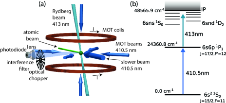
Figure 1: (color online) Experimental Setup (a) A focused Rydberg excitation laser is overlapped with a Ho MOT, resulting in depletion of the equilibrium atom number on resonance. (b) Energy level diagram. Rydberg atoms are created through two-photon excitation via $6s6p~{}^{1}P_{1}~{}F^{\prime}=12$, with the first photon provided by the 410.5 nm MOT beams.

Depletion spectroscopy is performed using two-photon excitation with $\sim$100 kHz linewidth lasers of a Ho MOT via the strong $4f^{11}(4I^{\circ}_{15/2})6s6p(^{1}P^{\circ}_{1})$ cooling transition, with a radiative line width of $\gamma/2\pi=32$ MHz. The experimental setup, shown schematically in Fig. 1(a), uses the apparatus detailed in Ref. Miao et al. (2014). An atomic beam of Ho is slowed using a 400 mW counter propagating beam, derived from a frequency doubled Ti:Sa laser, which is detuned in the range of $-210$ to $-330~{}\rm MHz$ from the $4f^{11}(4I^{\circ})6s^{2},F=11$ to $4f^{11}(4I^{\circ}_{15/2})6s6p(^{1}P^{o}_{1}),F^{\prime}=12$ transition at 410.5 nm. Atoms are loaded into a MOT formed at the intersection of three pairs of orthogonal beams with a detuning of -20 MHz and a total power of 400 mW, resulting in a saturation parameter of $I/I_{\mathrm{sat}}=1.06$. The equilibrium atom number is $7.5\times 10^{5}$ at a temperature $<500~{}\mu\rm K$, with a density of $2.2\times 10^{10}~{}{\rm cm}^{-3}$.

The MOT population is measured using a photodiode to monitor fluorescence. The collected fluorescence signal is amplitude modulated with an optical chopper, followed by lock-in detection, to suppress background electronic noise. At the two-photon resonance, atoms are excited to Rydberg states leading to increased loss of the MOT from decay into dark states and photoionization of the Rydberg atoms, reducing the equilibrium number. For each measurement, spectra are averaged over 50 repetitions and increasing and decreasing frequency ramps of the 413 nm laser are compared to verify that resonances are observed in both scan directions as well as to account for any hysteresis in the frequency ramp.

The MOT cooling laser is stabilized to an ultra high finesse ULE reference cavity (${\mathcal{F}}\sim 2\times 10^{6}$) mounted in vacuum and temperature controlled to $<\pm 10~{}\rm mK$, providing $<1$ MHz frequency drift for several weeks of measurements. The short term laser linewidth after locking to the reference cavity is estimated to be $\sim 100~{}\rm kHz$. Rydberg excitation is achieved using a frequency doubled 826 nm diode laser producing 3 mW at 413 nm, which is focused to a waist of $27~{}\mu\rm m$ and overlapped on the MOT. The 826 nm laser is locked to a Fabry-Perot reference cavity and scanned across 1-2 GHz with a scan period of about 10 s using the cavity piezo. The Fabry-Perot cavity uses a 10 cm long Invar spacer mounted inside a temperature controlled vacuum can. The cavity finesse is about 500 giving a cavity linewidth of about 3 MHz. The 826 nm laser is referenced to the slowly scanned cavity using a Pound-Drever-Hall locking schemeDrever et al. (1983) giving an estimated short term linewidth of 200 kHz at 413 nm. The vacuum can is temperature stabilized to better than 10 mK giving a long term frequency fluctuation of about 8 MHz at 413 nm. The combined frequency fluctuation of the two lasers, which is dominated by drift of the Invar reference cavity, is thus about 10 MHz or 0.0003 cm^-1.

The uncertainty in our determination of the energy of Rydberg levels is dominated by the uncertainty in our wavemeter measurement of the 413 nm laser light. The 410.5 nm MOT laser is referenced to an independent measurement of the centre of gravity transition frequency from $4f^{11}6s^{2},J=15/2$ to $4f^{11}6s6p,J^{\prime}=17/2$ is obtained with a $1~{}\rm m$ Fourier Transform Spectrometer calibrated against an Argon line using the experimental setup described in ref. Lawler et al. (2004). This gives an energy of 24360.790(1) cm^-1, which is combined with precise measurements of the ground Dankwort et al. (1974); Burghardt et al. (1982) and excited state Miao et al. (2014) hyperfine splittings to yield an absolute frequency of the MOT laser given by 730.31682(3) THz. This value is used to calibrate the wavemeter that measure the frequency of the scanned 413 nm Rydberg laser, resulting in a total uncertainty of 200 MHz or 0.007 cm^-1 in the absolute energy of the measured levels. Details of the energy calibration procedures are provided in the Appendix.

III Results and Discussion

From the $4f^{11}6s6p,J=17/2$ state it is possible to excite the atom to the $4f^{11}6sns$ and $4f^{11}6snd$ Rydberg states, with a total of 12 series accessible. Due to parity conservation, the coupling to the triplet series is expected to be very weak, reducing this to the seven odd parity singlet states $6sns(^{1}S_{0})$ J=15/2 and $6snd_{5/2,3/2}(^{1}D_{2})~{}J=15/2,17/2,19/2$ which are observed in the experiment. Figure 2 shows typical spectra for the $ns$ and $nd$ Rydberg series respectively, demonstrating both the relatively narrow ($\sim 30-60$ MHz) spectral width of the technique as well as resolution of the fine-structure splitting of the $nd$ state resonances in (b). As the oscillator strength decreases for higher $n$ whilst the ionization rates and available dark states increase, the absolute value of the depletion is a poor indicator of absolute transition strength, however this does provide relative strengths for closely spaced fine structure transitions. The number of fine structure states resolved for the $nd$ series varies between measurements due to the finite frequency range the second photon is scanned over, but for all datasets where the full range is included between 4-6 states are resolved, limited by the signal to noise for the weaker transitions.

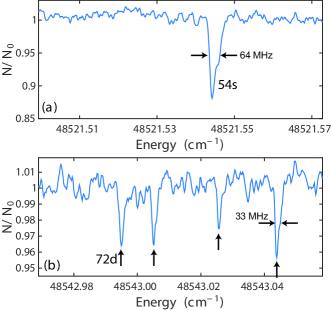
Figure 2: (Color Online) MOT Depletion Spectra (a) Isolated depletion line for the $54s$ state, resolved with a 60 MHz FWHM. (b) Multiple fine structure states are resolved for the $72d$ series, with the lowest energy level used to determine the series parameters as it is typically the strongest resolved line for each $n$.

The energy levels $E_{n}$ of the Rydberg series are described by the Rydberg-Ritz formula

$$E_{n}=E_{\mathrm{IP}}-\frac{\mathrm{Ry}}{[n-\delta(n)]^{2}},$$ (1)

where $E_{\mathrm{IP}}$ is the ionization potential which represents the series limit as $n\rightarrow\infty$ and $\delta(n)$ is the quantum defect for each series. For high-lying Rydberg states the quantum defect can be assumed to be independent of $n$, allowing extraction of a precision value for $E_{\mathrm{IP}}$ by fitting to the series convergence Worden et al. (1978). To verify which series the measured energy levels belong to, a Fano plot of $\delta$ modulo 1 against energy is used, as shown in Fig. 3. The measured energies then collapse into two distinct series, with the $ns$ series having a strong series perturbation around -1.5 THz and the $nd$ defects approximately constant for all $n$ for each of the different fine structure states. For the $nd$ data, the series with the largest defect is typically the strongest line and has been observed across the full range of measured energies. For this reason, only this fine structure state is used for analysis of the $nd$ defect, as the remaining satellite states are insufficiently discriminated to clearly identify their corresponding series correctly. As the strongest dipole matrix elements are for transitions to $6snd_{5/2}(^{1}D_{2}),J=19/2$, this is the most probable state being analyzed, from which we infer an inverted fine structure in the $nd$ series, as is observed in the Ho⁺ ionic ground state. Two additional states which could not be assigned to either $ns$ or $nd$ series were observed at 48530.035(7) and 48513.837(7) cm^-1, indicated by squares on Fig. 3.

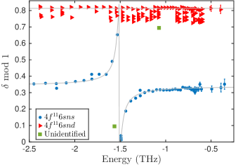
Figure 3: (Color Online) Fano plot of the quantum defect modulo one versus the energy of the Rydberg states. The quantum defect is constant as is expected for the d-series (red triangles) and shows a perturbation at around n=51 in the s-series (blue circles). Green squares indicate Rydberg levels of unknown configuration. Missing fine structure states on the $nd$ series arise due to finite measurement ranges, but have been observed for all $n$ states measured across the $\delta=0.7\ldots 0.85$ range. Error bars are indicated only when larger than symbol size.

The ionization potential is obtained using a least-squares fit to both the $ns$ and strong $nd$ series with $E>-1$ THz resulting in $E_{\mathrm{IP}}=48565.909(3)~{}$cm^-1, with both series converging to the $4f^{11}(^{4}I^{\circ}_{15/2})6s_{1/2},J=8$ Ho⁺ ground state. The uncertainty in $E_{\mathrm{IP}}$ is an improvement of three orders of magnitude over previous measurements Worden et al. (1978). In addition to obtaining the ionization potential, this fit also yields the asymptotic values of the quantum defects corresponding to 4.324(5) and 2.813(3) for the $ns$ and $nd$ series respectively. Whilst these defects are fitted modulo 1, the integer assignment is achieved by comparison to previous work Fano et al. (1976) which predicts that the quantum defect should be $\sim$4.3 for the $s$ series and $\sim$2.8 for the $d$ series from the variation of $\delta$ with atomic number. This is in good agreement with the defects calculated for the known energies of the $6s^{2}$ and $6s5d$ states.

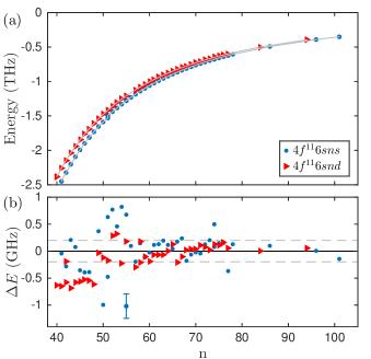
Figure 4: (Color Online) Rydberg state energy levels. (a) Measured energy levels for the $ns$ and $nd$ series, with solid lines calculated using fitted quantum defect parameters summarized in the text. (b) Fit residuals, yielding an r.m.s. residual of 200 MHz for $n>60$ away from the $51s$ series perturbation, in good agreement with the 200 MHz uncertainty (indicated by the dashed gray lines and plotted as a representative error bar).

For lower lying $n$ the quantum defect can be described by the Ritz formula $\delta(n)=\delta_{0}+\delta_{2}/(n-\delta_{0})^{2}$ Ritz (1903) which is used to fit the $nd$ series. Unfortunately the uncertainty in $\delta_{2}$ is an order of magnitude larger than the best-fit value, and the series is therefore best described by a constant defect of $\delta_{0}=2.813(3)$.

Due to the strong series perturbation in the $ns$ series, the data cannot be described by a single channel quantum defect model, and instead MQDT applies Seaton (1983). In this framework, the perturbation can be treated as coupling between two near-resonant series, resulting in a modification of the quantum defect of Seaton (1983); Roßnagel et al. (2012)

$$\delta(n)=\delta_{0}(n)-\frac{1}{\pi}\tan^{-1}\left[\frac{\Gamma/2}{(E_{n}-E_{j})}\right],$$ (2)

where $\Gamma$ is the spectral width and $E_{j}$ the energy of the interloper. Interestingly, despite the perturbation occurring below the first ionization potential associated with the Ho II ground state, the bound-bound series interaction can have a large spectral width comparable to a bound-continuum autoionization resonance Aymar et al. (1996).

$n$	Level Energy (cm-1)	$\delta$	$\Delta E$ (GHz)
41	48484.198	4.353	-0.04
42	48488.466	4.355	-0.28
43	48492.429	4.357	0.21
43	48492.537	4.357	3.46
44	48496.074	4.360	0.08
45	48499.442	4.364	-0.36
46	48502.578	4.370	-0.39
47	48505.407	4.377	-2.90
47	48505.490	4.378	-0.39
48	48508.150	4.391	-1.68
49	48510.713	4.417	0.37
50	48512.925	4.476	-1.00
51	48514.823	4.677	1.62
51	48516.151	4.011	-1.75
51	48516.181	4.017	-0.48
51	48516.207	4.022	0.63
52	48517.905	4.201	0.77
53	48519.736	4.257	0.46
54	48521.543	4.282	0.82
55	48523.194	4.294	-1.02
55	48523.250	4.295	0.68
56	48524.853	4.302	0.10
57	48526.379	4.308	-0.20
58	48527.843	4.312	0.15
59	48529.210	4.315	-0.12
60	48530.516	4.317	-0.02
61	48531.756	4.319	0.12
62	48532.929	4.320	0.13
63	48534.045	4.322	0.19
64	48535.100	4.323	0.11
65	48536.104	4.324	0.04
66	48537.066	4.324	0.17
67	48537.981	4.325	0.24
68	48538.837	4.326	-0.18
69	48539.671	4.326	-0.06
70	48540.465	4.327	-0.02
71	48541.222	4.327	-0.04
72	48541.951	4.327	0.13
73	48542.646	4.328	0.20
74	48543.305	4.328	0.08
74	48543.319	4.328	0.50
75	48543.943	4.328	0.15
76	48544.551	4.329	0.15
77	48545.118	4.329	-0.37
78	48545.694	4.329	0.13
86	48549.460	4.331	0.10
96	48552.850	4.331	0.01
101	48554.161	4.332	-0.14

Table 1: Measured energies for the $4f^{11}6sns$ series, accurate to 0.007 cm^-1 with best-fit quantum defect $\delta$ determined from Eq. (2) using $\delta_{0}=4.341(2)$, $\Gamma=6.9(3)$ GHz and $E_{j}=48515.47(4)$ cm^-1. The residuals relative to the Rydberg-Ritz formula are labeled $\Delta E$. Multiple $n=51$ states appear due to the series perturbation, as well as a number of additional weak doublets indicated by an asterix (*).

The fitted defect is shown in Fig. 3 which accurately reproduces the observed perturbations, resulting in parameters $\delta_{0}=4.341(2)$, $\Gamma=6.9(3)$ GHz and $E_{j}=48515.47(4)$ cm^-1. The perturbing series is unknown, but likely has the same $4f^{11}$ inner electronic configuration due to the strength of the interaction. Around this resonance the $ns$ series is observed to split into doublets, resulting in four separate states being identified as $n=51$ due to fine structure splitting of the series interloper. Weak doublets are also observed for a few other $s$ states ($n=43,47,74$), due either to much weaker inter-series resonances or potentially singlet-triplet mixing within the $ns$ series. Above the ionization potential, we also observe a strong autoionization resonance at 48567.958(1) cm^-1 with a FWHM of 9(1) GHz. This lies 60 GHz above the first ionization potential, and thus is not an excitation to the $J=7$ fine structure state of the ionic core which lies 637. cm^-1 above $E_{\mathrm{IP}}$ Martin et al. (1978).

$n$	Energy (cm-1)	$\Delta E$ (GHz)	Level Energies (cm-1)
40	48486.532	-0.63	48486.503	48486.720	48486.781
41	48490.634	-0.64	48490.700	48490.861
42	48494.441	-0.19	48494.428	48494.525	48494.556	48494.583
43	48497.936	-0.68	48498.149
44	48501.200	-0.57
45	48504.231	-0.55
46	48507.054	-0.52	48507.126
47	48509.687	-0.55
48	48512.145	-0.61	48512.215	48512.295	48512.344
49	48514.466	-0.03	48514.563
50	48516.620	-0.13	48516.711	48516.740	48516.782
51	48518.643	-0.17	48518.752	48518.789
52	48520.560	0.28	48520.641	48520.642	48520.668	48520.702
53	48522.351	0.32	48522.398	48522.427	48522.445	48522.452	48522.461
54	48524.019	-0.22	48524.079	48524.107
55	48525.622	0.17	48525.705	48525.732
56			48527.144	48527.169	48527.191	48527.216
57	48528.526	-0.29	48528.563	48528.606
58	48529.884	0.18	48529.871	48529.906	48529.920	48529.930	48529.949
59	48531.145	-0.10
60	48532.348	-0.19
61	48533.495	-0.07
62	48534.581	-0.06
63	48535.613	-0.07
64	48536.598	-0.00	48536.624	48536.643	48536.654	48536.669
65	48537.537	0.13	48537.562	48537.592	48537.606
66	48538.417	-0.20
67	48539.270	-0.10	48539.295	48539.321	48539.335
68	48540.085	0.02	48540.107	48540.127	48540.139
69	48540.860	0.03
70	48541.601	0.04
71	48542.310	0.10	48542.319	48542.339	48542.368
72	48542.987	0.07	48543.005	48543.026	48543.036
73	48543.634	0.02	48543.651
74	48544.259	0.13	48544.297
75	48544.854	0.11	48544.890	48544.899
76	48545.427	0.16	48545.444	48545.461	48545.469
77	48545.972	0.06	48545.988	48546.007	48546.015
84	48549.261	0.00
94	48552.714	0.05

Table 2: Measured states for the $4f^{11}6snd$ series, accurate to 0.007 cm^-1. The first column represents the dominant series used for determination of the quantum defect and IP for the series. The residuals relative to the Rydberg-Ritz formula are labeled $\Delta E$, with $\delta_{0}=2.813(3)$. The remaining levels are weaker fine structure states which could not be unambiguously assigned to a common series.

Figure 4 shows the resulting energy residuals from the $ns$ and $nd$ fits, which with the exception of the increased error around the $51s$ series perturbation results in an r.m.s. residual of 200 MHz for $n>60$, in good agreement with the 200 MHz uncertainty in determination of the absolute energy of the levels. Absolute energies and residuals for each state are given in Tables 1 and 2, in addition to energies of the other $nd$ fine structures states.

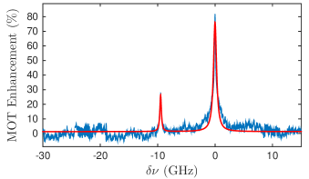
Figure 5: (Color Online) Enhancement of the MOT number as a function of detuning from $\nu=724.2662(2)$ THz due to repumping population from a long lived metastable state back to the ground state cooling cycle, with a resolved hyperfine splitting of 9.47(1) GHz.

IV MOT Enhancement Resonance

Alongside the depletion resonances, a strong enhancement feature was observed resulting in up to 80% increase in the MOT atom number at $\nu=724.2662(2)$ THz, as shown in Fig. 5. The two enhancement features have a FHWM of 600 MHz and are spaced by 9.47(1) GHz, consistent with transitions between different hyperfine states. Enhancement of the MOT arises due to repumping population either from uncoupled ground state hyperfine levels or long-lived metastable excited states back into the $F=11$ ground state which is cooled in the MOT. The peak enhancement wavelength is independent of the MOT detuning, verifying that this effect arises from a single photon repump transition which can be exploited to create large atomic samples. The closest matching transition from published line data is from $4f^{10}(^{5}I_{8})5d_{5/2}6s^{2},J=17/2$ to $4f^{10}5d6s6p,J=17/2$ Kröger et al. (1997), which has a frequency of 724.350 THz, within 10 GHz of the measured resonance.

V Summary

In summary we have measured 162 odd-parity Rydberg states belonging to the $4f^{11}6sns$ and $4f^{11}6snd$ series using MOT depletion spectroscopy, providing the first energy resolved Rydberg spectra for neutral Ho. Analysis of the measured levels yields a significantly improved determination of the first ionization potential of $E_{\mathrm{IP}}=48565.939(4)$ cm^-1, as well as asymptotic quantum defects for the $ns$ and $nd$ series of 4.341(2) and 2.813(3) respectively. These data provide an important reference for testing ab initio theories predicting the energy levels of complex atoms. The observation of regular $ns$ and $nd$ series without strong perturbations for most $n$ in the range $40\leq n\leq 101$ suggests that we can expect to find long lived Rydberg states suitable for creating collectively encoded quantum registers Saffman and Mølmer (2008). Determination of Rydberg lifetimes and interaction strengths will be the subject of future work. In addition to Rydberg levels, a strong repump transition has been identified enabling a significant increase in MOT atom number. This will be useful for preparing large, dense atomic samples as a starting point for creation of a dipolar Bose-Einstein condensate Lahaye et al. (2009); Lu et al. (2011); Aikawa et al. (2012) exploiting the large 9 $\mu_{\mathrm{B}}$ magnetic moment.

Appendix A Energy Level Calibration

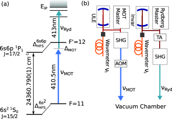
Figure 6: Holmium Energy Levels. (a) MOT and Rydberg laser transitions with respect to the ground state energy level and hyperfine splitting. (b) Laser setup showing cavity locks, wavelength measurement and additional frequency shift from AOMs on the cooling laser. A wavemeter is used to measure the laser frequencies $\nu_{1,2}$ before they are doubled and sent to the atoms.

To provide accurate energy levels of the measured Rydberg states we use an independent measurement to determine the absolute frequency of the MOT laser, which is stabilized to the TEM₀₀ mode of a high finesse ULE cavity providing a stable long term frequency reference. Figure 6(a) shows the relevant energy levels and splittings used in the experiment, whilst the laser setup is shown in (b). The centre of mass frequency for the $4f^{11}6s^{2}~{}^{1}S_{0}~{}J=15/2$ to $4f^{11}6s6p~{}^{1}P_{1}~{}J=17/2$ transition is determined by the 1m Fourier Transform Spectrometer at the National Solar Observatory using the setup detailed in ref. Lawler et al. (2004). High resolution spectra from a Ho-Ar hollow cathode lamp are recorded, using lines in the well known ArII series Learner and Thorne (1988); Whaling et al. (2002) for calibration to give a transition frequency of $E_{6s^{2}\rightarrow 6s6p}=24360.790(1)~{}\rm cm^{-1}$ which is 0.02 $\rm cm^{-1}$ less than the value in the NIST tables Martin et al. (1978).

For the cooling transition from $F=11$ to $F^{\prime}=12$, the hyperfine splitting of the ground and excited states are calculated from measurements of the hyperfine constants giving $\Delta_{\mathrm{F=11}}^{6s^{2}}=20.589319(1)$ GHz Dankwort et al. (1974); Burghardt et al. (1982) $\Delta_{\mathrm{F^{\prime}=12}}^{6s6p}=19.33(1)$ GHz Miao et al. (2014). The frequency of the MOT transition can then be calculated from

$$\nu_{\mathrm{MOT}}=E_{6s^{2}\rightarrow 6s6p}+\Delta_{\mathrm{F^{\prime}=12}}^{6s6p}-\Delta_{\mathrm{F=11}}^{6s^{2}}+\Delta_{\mathrm{MOT}},$$ (3)

where $\Delta_{\mathrm{MOT}}=-22(2)$ MHz is the detuning from resonance determined from spectroscopy of the atomic beam, giving $\nu_{\mathrm{MOT}}=730.31682(3)$ THz. Accounting for the double pass acousto-optic modulator (AOM) at 50 MHz and frequency doubling of the SHG, the frequency of the master Ti:Sa laser locked to the cavity is given by $\nu_{\mathrm{ref}}=365.15836(2)$ THz. For each measurement, the wavelength of this laser ($\nu_{1}$) is recorded on a wavemeter to determine the wavemeter offset $\delta\nu=\nu_{\mathrm{ref}}-\nu_{1}$. The Rydberg energy levels are then calculated from measuring the Rydberg master laser frequency ($\nu_{2}$) before the doubling cavity on the same wave meter, resulting in $\nu_{\mathrm{Ryd}}=2(\nu_{2}+\delta\nu)$, with the absolute energy above the ground state given by

$$E_{\mathrm{Ryd}}=\Delta_{\mathrm{F=11}}^{6s^{2}}+\nu_{\mathrm{MOT}}+\nu_{\mathrm{Ryd}},$$ (4)

resulting in a total uncertainty of 200 MHz on the final energy reading.