Flipped GUT Inflation

Abstract

We analyse the prospects for constructing hybrid models of inflation that provide a dynamical realisation of the apparent closeness between the supersymmetric GUT scale and the possible scale of cosmological inflation. In the first place, we consider models based on the flipped SU(5)$\times$U(1) gauge group, which has no magnetic monopoles. In one model, the inflaton is identified with a sneutrino field, and in the other model it is a gauge singlet. In both cases we find regions of the model parameter spaces that are compatible with the experimental magnitudes of the scalar perturbations, $A_{s}$, and the tilt in the scalar perturbation spectrum, $n_{s}$, as well as with an indicative upper limit on the tensor-to-scalar perturbation ratio, $r$. We also discuss embeddings of these models into SO(10), which is broken at a higher scale so that its monopoles are inflated away.

[wrap] John Ellis^1,2, Tomás E. Gonzalo³, Julia Harz³, Wei-Chih Huang³

¹Theoretical Particle Physics and Cosmology Group, Department of Physics, King’s College London, London WC2R 2LS, United Kingdom
²Theory Division, CERN, CH-1211 Geneva 23, Switzerland
³Department of Physics and Astronomy, University College London, London WC1E 6BT, United Kingdom

KCL-PH-TH/2014-49, LCTS/2014-50, CERN-PH-TH/2014-241

1 Introduction

It has long been recognised that the naive extrapolation of the gauge coupling strengths measured at accessible energies is consistent with simple supersymmetric models of grand unification at an energy scale $M_{GUT}\sim 2\times 10^{16}$ GeV.[1, 2, 3, 4] In parallel, it has also long been apparent that successful cosmological inflation probably requires new physics at some energy scale far beyond that of the Standard Model. Assuming the value of the amplitude $A_{s}$ of scalar perturbations in the cosmic microwave background radiation (CMB) measured by the Planck Collaboration, $A_{s}=(2.19\pm 0.11)\times 10^{-9}$ [5], one finds within the usual slow-roll inflationary paradigm that the energy density during inflation has the value

$$V_{\phi}^{1/4}=2\times 10^{16}\left(\frac{r}{0.15}\right)^{1/4},$$ (1)

where $r$ is the ratio of the amplitude of tensor perturbations relative to scalar perturbations. The Planck data are compatible with $r\sim 0.1$, which would correspond to a remarkable coincidence between $M_{GUT}$ and $V_{\phi}^{1/4}$. The slow dependence of $V_{\phi}^{1/4}$ on $r$ implies a value of $r$ two orders of magnitude smaller, such as found in the attractive $R+R^{2}$ model of Starobinsky [6], would still correspond to a value of $V_{\phi}^{1/4}$ within a factor $\sim 2$ of the supersymmetric GUT scale.

Accordingly, it is natural to speculate that there may be some connection between the ideas of cosmological inflation and grand unification. Perhaps inflation was generated along some direction in the space of grand unified Higgs fields? In this case, the requirement of successful inflation might impose some interesting restrictions on the possible structure of a supersymmetric grand unified theory (GUT). For example, how does one ensure the absence of GUT monopoles, or the suppression of their relic density? Conversely, the requirement of consistency with grand unification might provide some interesting constraint on inflationary model-building, perhaps leading to some interesting predictions for inflationary observables such as $A_{s}$, $r$ and the tilt of the scalar perturbation spectrum, $n_{s}$.

Interest in the possible connection between supersymmetric GUTs and inflation was greatly stimulated by the observation in the BICEP2 experiment of substantial B-mode polarisation in the CMB [7]. If this were mainly due to primordial tensor perturbations generated during inflation, it would point to a value of $r$ close to the Planck upper limit, and confirm the remarkable coincidence between the energy scales of inflation and grand unification. However, recent data from the Planck Collaboration [8] indicate that there is substantial pollution of the BICEP2 B-mode signal by foreground dust, which might even explain the majority of the signal. Even in this case, the great increase in sensitivity achieved by the BICEP2 Collaboration and the prospects for future experiments such as the Keck Array encourage us to hope that experiments on B-mode polarisation will soon attain the sensitivity required to place interesting constraints on GUT models of inflation.

A general approach to the construction of GUT inflationary models was taken in a recent paper by Hertzberg and Wilczek [9]. These authors did not consider a specific GUT framework, taking instead a rather phenomenological attitude to the possible structure of the effective potential during the inflationary epoch. We here adopt a more focused approach within the class of inflationary models, known as hybrid inflation, first proposed by Linde [10, 11, 12, 13, 14, 15, 16, 17, 18, 19]. In this work, the hybrid inflationary potential is used as a dynamical source of GUT symmetry breaking, and thereby relate the unification scale to value of the scalar potential at the start of inflation. We seek realisations of this scenario within the frameworks of specific (relatively) simple GUT models based on minimal gauge groups, namely flipped SU(5)$\times$U(1) and SO(10) . In the former case, there are no GUT monopoles and the model can be derived in a natural way from weakly-coupled string theory. In the latter case, there are GUT monopoles, and one must ensure that their cosmological density is suppressed during an inflationary epoch that occurs subsequent to SO(10) symmetry breaking.

In Section 2 we study two distinct flipped SU(5)$\times$U(1) scenarios for GUT inflation. In one, the inflaton is identified with a neutrino field contained within a 10-dimensional representation of SU(5), and in the other the inflation is identified with a singlet field. In both scenarios, we find regions of parameter space where the experimental values of $A_{s}$ and $n_{s}$ are obtained, and the values of $r$ are compatible with indicative upper limits from Planck. We also discuss in Section 3 how these models may be embedded within SO(10) models. The simplest option is simply to break SO(10) $\to$ SU(5)$\times$U(1) via a 45-dimensional adjoint representation of SO(10), but this cannot be obtained from simple compactifications of weakly-coupled string theory, so we also consider a flipped SO(10)$\times$U(1) version. Finally, our conclusions are summarised in Section 4.

2 Minimal GUT Inflation: Flipped SU(5)$\times$U(1)

The simplest and first proposal for a Grand Unified Theory that embeds the standard model gauge groups SU(3)$\times$SU(2)$\times$U(1) into a single semisimple group $G$ is the SU(5) model that Georgi and Glashow proposed in 1974 [23]. However, this kind of GUT model, in which the electromagnetic U(1) group is embedded in a simple group, necessarily contains magnetic monopoles [24, 25]. Depending on the scale at which GUT symmetry breaking occurs, the cosmological abundance of these monopoles may exceed the experimental limits. The density of magnetic monopoles would have been diluted by the inflationary expansion if the GUT symmetry-breaking phase transition occurred before inflation, but the density of magnetic monopoles would be too large if the symmetry breaking took place after inflation, overclosing the Universe [26].

One way to circumvent the magnetic monopole problem is to postulate a non-semi-simple group. In this case, if the abelian electromagnetic U(1) group is not entirely contained with a semi-simple group factor, the theory does not contain magnetic monopoles. One such model is the flipped SU(5)$\times$U(1) model [27, 28, 29, 30, 31, 32]  (for a synoptic review, see [33]), in which the electromagnetic U(1) is a linear combination of generators in the SU(5) and U(1) factors. This model has been studied extensively in the literature because of its many advantages. For instance, it features a natural Higgs doublet-triplet splitting mechanism, can give masses to neutrinos through the seesaw mechanism and does not contain troublesome $d=5$ proton decay operators. Moreover, since it does not require adjoint or larger Higgs representations, the flipped SU(5)$\times$U(1) model can be obtained from the weakly-coupled fermionic formulation of string theory [34, 35, 36, 37].

The simplest flipped SU(5)$\times$U(1) model contains the following particle content [30, 31]:

• The Standard Model (SM) matter content is embedded in $\hat{10}_{F}$, $\hat{\bar{5}}_{F}$, and $\hat{1}_{F}$ representations, with U(1) charges of $1$, $-3$, and $5$, respectively.

• The Higgs bosons that break electroweak symmetry are in $\hat{5}_{H_{u}}$ and $\hat{\bar{5}}_{H_{d}}$ representations.

• The breaking of SU(5)$\times$U(1) $\to$ SU(3)${}_{c}\times$SU(2)${}_{L}\times$U(1)_Y arises from expectation values for $\hat{10}_{H}$ and $\hat{\bar{10}}_{H}$ representations that can appear in simple string models.

• A singlet field $\hat{1}_{S}$ is introduced to provide in a natural way the $\hat{5}_{H_{u}}\hat{\bar{5}}_{H_{d}}$ mixing that is required for successful electroweak symmetry breaking.

• Optionally, one can include three generations of sterile neutrinos $\hat{1}_{N}^{i}$ that induce a seesaw mechanism for the neutrino masses. This effect can also be reproduced by effective non-renormalizable operators if the theory is embedded into a larger theory.

The most general superpotential for the flipped SU(5)$\times$U(1) model, in the absence of sterile neutrinos, is

$$W=~{} y_{u}\hat{10}_{F}\hat{10}_{F}\hat{5}_{H_{u}}+y_{d}\hat{10}_{F}\hat{\bar{5}}_{F}\hat{\bar{5}}_{H_{d}}+y_{e}\hat{\bar{5}}_{F}\hat{1}_{F}\hat{5}_{H_{u}}$$

$$+\lambda_{u}\hat{10}_{H}\hat{10}_{H}\hat{5}_{H_{u}}+\lambda_{u}^{\prime}\hat{10}_{F}\hat{10}_{H}\hat{5}_{H_{u}}+\lambda_{d}\hat{\bar{10}}_{H}\hat{\bar{10}}_{H}\hat{\bar{5}}_{H_{d}}+\lambda_{d}^{\prime}\hat{10}_{H}\hat{\bar{5}}_{F}\hat{\bar{5}}_{H_{d}}$$

$$+\lambda_{F}\hat{10}_{F}\hat{\bar{10}}_{H}\hat{1}_{S}+\lambda_{5}\hat{5}_{H_{u}}\hat{\bar{5}}_{H_{d}}\hat{1}_{S}+\lambda_{10}\hat{10}_{H}\hat{\bar{10}}_{H}\hat{1}_{S}+\lambda_{S}\hat{1}_{S}\hat{1}_{S}\hat{1}_{S}$$

$$+\mu_{F}\hat{10}_{F}\hat{\bar{10}}_{H}+\mu_{5}\hat{5}_{H_{u}}\hat{\bar{5}}_{H_{d}}+\mu_{10}\hat{10}_{H}\hat{\bar{10}}_{H}+\mu_{S}\hat{1}_{S}\hat{1}_{S}+M_{S}^{2}\hat{1}_{S}\,,$$ (2)

which includes both dimensionless and dimensionful couplings.

Symmetry breaking from flipped SU(5)$\times$U(1) to the Standard Model happens whenever $\langle\nu^{c}_{H}\rangle\neq 0$ where $\nu^{c}_{H}\in\hat{10}_{H}$, and/or $\langle\bar{\nu}^{c}_{H}\rangle\neq 0$ where $\bar{\nu}^{c}_{H}\in\hat{\bar{10}}_{H}$. In the absence of supersymmetry breaking, there are no tachyonic mass terms for neither $\nu^{c}_{H}$ nor $\bar{\nu}^{c}_{H}$. However, if supersymmetry is broken above the GUT scale, as in supergravity models [38, 39], one may obtain soft SUSY breaking (SSB) terms such as

$$V_{SSB}=~{}(A_{ijk}y_{ijk}\phi^{i}\phi^{j}\phi^{k}+B_{ij}\mu_{ij}\phi^{i}\phi^{j}+c.c.)+m_{i}^{2}|\phi^{i}|^{2}$$ (3)

at some high renormalisation scale $\mu>M_{GUT}$. Renormalization effects due to the couplings $\lambda_{u}$, $\lambda_{d}$ and/or $\lambda_{F}$ may then drive the SSB masses $m_{10_{H}}^{2}$ and $m_{\bar{10}_{H}}^{2}$ tachyonic at a large scale $\mu\sim M_{GUT}$. In this case the fields $\nu^{c}_{H}$ and/or $\bar{\nu}^{c}_{H}$ acquire vevs, triggering the symmetry breaking SU(5)$\times$U(1) $\to$ SU(3)${}_{c}\times$SU(2)${}_{L}\times$U(1)_Y [30, 31].

Two different inflationary scenarios can be considered within this flipped SU(5)$\times$U(1) framework: the inflaton may be taken to be either a right-handed sneutrino, $\nu^{c}\in\hat{10}_{F}$, or a singlet $\hat{1}_{S}$. Sneutrino inflationary models have been studied extensively in the literature [40, 41, 42, 43, 44, 45, 46, 47, 48]. At the time of writing we are unaware of any study of sneutrino-driven inflation in a flipped SU(5)$\times$U(1) model, though this possibility was suggested in [49]. Thus, in section 2.1 we discuss the steps required to build a hybrid inflationary model driven by such a singlet (right-handed) sneutrino. Then, in section 2.2 we analyse the second scenario in which the inflaton is a singlet under the GUT group. We show that, if one abandons the idea of sneutrino inflation, the constraints are much looser, and one can even build inflationary potentials with higher powers of the inflation field that are consistent with the CMB measurements, along the lines discussed in [50].

2.1 Flipped Sneutrino Inflation

In order to realise sneutrino inflation driven by the component $\nu^{c}\in\hat{10}_{F}$, we focus on the following superpotential terms in (2) that involve the $\hat{10}_{F}$, $\hat{10}_{H}$ and $\hat{\bar{10}}_{H}$ representations:

$$W\supset~{} \lambda_{F}\hat{10}_{F}\hat{\bar{10}}_{H}\hat{1}_{S}+\mu_{F}\hat{10}_{F}\hat{\bar{10}}_{H}+\mu_{10}\hat{10}_{H}\hat{\bar{10}}_{H}+\lambda_{10}\hat{10}_{H}\hat{\bar{10}}_{H}\hat{1}_{S}\,.$$ (4)

Other terms in (2) include other superfields and are irrelevant for the analysis of inflation. For example, the antisymmetric coupling $\hat{10}_{F}\hat{10}_{H}\hat{5}_{H_{u}}$ will not contribute because it contains components of the fields other than $\nu^{c}$, $\nu^{c}_{H}$ and $\bar{\nu}^{c}_{H}$. The scalar potential of this model contains the $F$-terms derived from this superpotential and the corresponding $D$-terms. The latter add quartic couplings to the scalar potential, for both the inflaton and the GUT symmetry-breaking fields. In general, it is possible to create a viable model for inflation with powers higher than quadratic in the inflaton field. However, as discussed in [50], that would require the quartic coupling to be small: $\lambda\sim 10^{-7}-10^{-8}$. This is not the case for the $D$-terms, whose coupling is proportional to $g\sim 0.1-1$. Thus, we introduce another representation $\hat{\bar{10}}_{F}$ with the superpotential couplings

$$W\supset\bar{\lambda}_{F}\hat{\bar{10}}_{F}\hat{10}_{H}\hat{1}_{S}+\bar{\mu}_{F}\hat{\bar{10}}_{F}\hat{10}_{H}\,,$$ (5)

to ensure the cancellation of the $D$-term contribution of the inflaton field.

For the following discussion, we identify the fields as follows: $h=\nu^{c}_{H}\in\hat{10}_{H}$ , $\bar{h}=\bar{\nu}^{c}_{H}\in\hat{\bar{10}}_{H}$, $\phi=\nu^{c}\in\hat{10}_{F}$, $\bar{\phi}=\bar{\nu}^{c}\in\hat{\bar{10}}_{F}$, which allows for a direct comparison with [9]. With this notation, the $F$-term scalar potential can be written as

$$V_{F}=~{} 4(\mu_{10}^{2}+\bar{\mu}_{F}^{2})h^{2}+4(\mu_{10}^{2}+\mu_{F}^{2})\bar{h}^{2}+4\lambda_{10}^{2}h^{2}\bar{h}^{2}$$

$$+4(2\lambda_{10}h\bar{h})(\lambda_{F}\bar{h}\phi+\bar{\lambda}_{F}h\bar{\phi})+8\mu_{10}(\mu_{F}h\phi+\bar{\mu}_{F}\bar{h}\bar{\phi})$$

$$+4(\bar{\lambda}_{F}h\bar{\phi}+\lambda_{F}\bar{h}\phi)^{2}+4\mu_{F}^{2}\phi^{2}+4\bar{\mu}_{F}\bar{\phi}^{2}.$$ (6)

The corresponding $D$-term, including both Abelian and non-Abelian contributions, has the general form

$$V_{D}\propto(\phi^{2}-\bar{\phi}^{2}+h^{2}-\bar{h}^{2})^{2}\,.$$ (7)

To cancel the $\phi$ and $\bar{\phi}$ contributions to the $D$-term during inflation, it is sufficient to set $\phi^{\ast}=\bar{\phi}^{\ast}$  at the beginning of inflation and $\mu_{F}=\bar{\mu}_{F}$ so that the equations of motion are the same for $\phi$ and $\bar{\phi}$, at least during inflation. The last remaining pieces of the scalar potential are the SSB terms, as described in (3). We consider here only the SSB masses for $\hat{10}_{H}$ and $\hat{\bar{10}}_{H}$, since they are needed to trigger GUT symmetry breaking. The rest of SSB terms are assumed to be much smaller than the GUT scale, and therefore are neglected in the following. Due to the strong running of $m_{h}$ and $m_{\bar{h}}$, starting from their UV non-tachyonic values, they can easily become tachyonic at $M_{GUT}$, so that

$$V_{SSB}=-m_{h}^{2}|h|^{2}-m_{\bar{h}}^{2}|\bar{h}|^{2}\,,$$ (8)

where $m_{h}^{2},m_{\bar{h}}^{2}>0$.

With the scalar potential $V=V_{F}+V_{D}+V_{SSB}$, inflation starts at $\phi=\phi^{\ast}\gtrsim M_{P}$, for which we require $h$ and $\bar{h}$ to be stable around $h=\bar{h}=0$. The potential, however, does not have a minimum at the origin, unless $\mu_{10}=0$. Therefore, we set $\mu_{10}=0$, so that the potential is stable at $h=\bar{h}=0$ during inflation. Thus, the inflationary potential reads

$$V_{\phi}=4\mu_{F}^{2}\phi^{2}+4\bar{\mu}_{F}^{2}\bar{\phi}^{2}.$$ (9)

The free parameters $\mu_{F}$ and $\bar{\mu}_{F}$ of the inflationary observables can be determined from the experimental values of the the scalar amplitude $A_{s}$, the spectral index $n_{s}$, and the tensor-to-scalar ratio $r$.

In a single-field inflationary model, these parameters are given by

$$A_{s} =\frac{V(\phi^{\ast})}{24\pi^{2}M^{4}_{\mathrm{P}}\epsilon(\phi^{\ast})},$$

$$n_{s} =1-6\epsilon(\phi^{\ast})+2\eta(\phi^{\ast}),$$

$$r =16\epsilon(\phi^{\ast})$$ (10)

in the slow-roll limit [51], where the corresponding slow-roll parameters are given by

$$\epsilon(\phi) =\frac{M^{2}_{\mathrm{P}}}{2}\left(\frac{V^{\prime}(\phi)}{V(\phi)}\right)^{2}$$

$$\eta(\phi)$$

The number of e-foldings is given by where $\phi_{\rm end}$ corresponds to the value of $\phi$ when the slow-roll limit becomes invalid. Using (LABEL:efoldings), we can rewrite the slow-roll parameters in (LABEL:slowrollparameters) as functions of the number of e-foldings. This allows us to identify the regions of parameter space compatible with the measured values of the observables (10) in terms of the number of e-foldings and the parameters $\mu_{F}$ and $\bar{\mu}_{F}$.

However, the potential in (9) is actually a two-field inflation model, for which the influence of isocurvature modes could be significant [54, 55] , unlike the case of single-field inflation. However, as was discussed above, in order to cancel the $D$-terms during the inflationary era, it is necessary to impose $\mu_{F}=\bar{\mu}_{F}$. This cancels exactly the contributions from isocurvature perturbations, which depend on the difference $\mu^{2}_{F}-\bar{\mu}^{2}_{F}$, and would be important if this were not the case [67]. In the context of two-field inflation with the $\delta N$-formalism, the slow-roll parameters become [54]

$$\epsilon(\phi^{\ast},\bar{\phi}^{\ast}) =\epsilon(\phi^{\ast})+\epsilon(\bar{\phi}^{\ast}),$$

$$\zeta(\phi^{\ast},\bar{\phi}^{\ast}) =\frac{V(\phi^{\ast},\bar{\phi}^{\ast})^{2}}{\tfrac{V(\phi^{\ast})^{2}}{\epsilon(\phi^{\ast})}+\tfrac{V(\bar{\phi}^{\ast})^{2}}{\epsilon(\bar{\phi}^{\ast})}},$$

$$\eta(\phi^{\ast},\bar{\phi}^{\ast}) =\left(\frac{\eta(\phi^{\ast})}{\epsilon(\phi^{\ast})}V(\phi^{\ast})^{2}+\frac{\eta(\bar{\phi}^{\ast})}{\epsilon(\bar{\phi}^{\ast})}V(\bar{\phi}^{\ast})^{2}\right)\frac{\zeta(\phi^{\ast},\bar{\phi}^{\ast})}{V(\phi^{\ast},\bar{\phi}^{\ast})^{2}},$$ (11)

where the full potential in (9) is sum separable and can be divided into terms involving only $\phi$ or $\bar{\phi}$, i.e., $V(\phi,\bar{\phi})=V(\phi)+V(\bar{\phi})$. Moreover, the slow-roll parameters are defined as

$$\epsilon(\phi)=\frac{M^{2}_{\mathrm{P}}}{2}\left(\frac{V^{\prime}(\phi)}{V(\phi,\bar{\phi})}\right)^{2}\,,\,\,\,\eta(\phi)=M^{2}_{\mathrm{P}}\left(\frac{V^{\prime\prime}(\phi)}{V(\phi,\bar{\phi})}\right)\,.$$ (12)

and similarly for $\epsilon(\bar{\phi})$ and $\eta(\bar{\phi})$. Then, the inflationary observables can be expressed as

$$A_{s} =\frac{V(\phi^{\ast},\bar{\phi}^{\ast})}{24\pi^{2}M_{P}^{4}\zeta(\phi^{\ast},\bar{\phi}^{\ast})}\,,$$

$$n_{s} =1-2\epsilon(\phi^{\ast},\bar{\phi}^{\ast})-4\zeta(\phi^{\ast},\bar{\phi}^{\ast})+2\eta(\phi^{\ast},\bar{\phi}^{\ast})\,,$$

$$r =16\zeta(\phi^{\ast},\bar{\phi}^{\ast})\,,$$ (13)

with

$$N_{e}=\frac{1}{M^{2}_{\mathrm{P}}}\int_{\phi_{\rm end}}^{\phi^{\ast}}\frac{V(\phi)}{V^{\prime}(\phi)}\mathrm{d}\phi+\frac{1}{M^{2}_{\mathrm{P}}}\int_{\phi_{\rm end}}^{\phi^{\ast}}\frac{V(\bar{\phi})}{V^{\prime}(\bar{\phi})}\mathrm{d}\bar{\phi}\,.$$ (14)

We use these expressions to explore the parameter space in the coupling $\mu_{F}$ and the number of e-foldings $N_{e}$ that reproduce the required values of the observables $A_{s},n_{s}$ and $r$. As we have chosen $\phi^{*}=\bar{\phi}^{*}$ and $\mu_{F}=\bar{\mu}_{F}$ in order to cancel the $\phi$ and $\bar{\phi}$ contributions to the $D$-term during inflation, our model reduces to an effective single-field model ($\psi=\sqrt{2}\phi=\sqrt{2}\bar{\phi}$) during inflation. Thus, we can write simple expressions for the number of e-folds in terms of the corresponding observables

$$N_{e}^{A_{s}}=\frac{1}{4}\sqrt{\frac{12M^{2}_{\mathrm{P}}\pi^{2}A_{s}^{\mathrm{obs}}}{\mu^{2}_{F}}},\quad\qquad N_{e}^{r}>\frac{8}{r_{\mathrm{obs}}},\quad\qquad N_{e}^{n_{s}}=\frac{2}{1-n_{s}^{\mathrm{obs}}}.$$ (15)

For our analysis of the remaining parameters of our model, we use the experimental values given in Table 1. We assume the recent experimental values from the Planck collaboration [5] for the scalar amplitude $A_{s}$ and the spectral index $n_{s}$. Regarding the tensor-to-scalar ratio, the recent observation of B-mode polarisation of the CMB by the recent BICEP2 result [7] would suggest a relatively large value $r=0.20^{+0.07}_{-0.05}$ in the absence of dust. The BICEP2 collaboration estimated the possible reduction in $r$ implied by dust contamination, but a recent Planck study of the galactic dust emission [8] suggests that this may be more important than estimated by BICEP2. It may be that the polarized galactic dust emission accounts for most of the BICEP2 signal, although further study is needed to settle down this issue. To be conservative, we set the upper limit on $r$ shown in Table 1, a compromise between the BICEP2 result and the limit set by Planck $r<0.16$ at the 95% CL when allowing running in $n_{s}$ [5].

$A_{s}$	$n_{s}$	r
$(2.19\pm 0.11)\times 10^{-9}$	$0.9603\pm 0.0073$	$<0.16$

Table 1: Table of experimental constraints from [5].

We show in Fig. 1 the region of the parameter $\mu_{F}$ ($=\bar{\mu}_{F}$) and the number of e-foldings $N_{e}$ that is allowed by these cosmological observables. The strongest constraint comes from the scalar amplitude $A_{s}$ (in blue), which is a rather thin band, whereas the spectral index $n_{s}$ (shaded pink) allows a broad band of the parameter space. Within this model, the tensor-to-scalar perturbation ratio $r$ (shaded green, with stripes), sets a lower bound on the number of e-foldings.

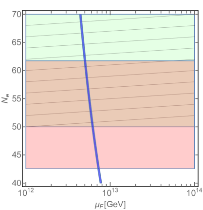
Figure 1: The $(\mu_{F}=\bar{\mu}_{F},N_{e})$ plane, showing the blue strip that is compatible with the experimental value of the scalar amplitude $A_{s}$, a band (shaded pink) that is compatible with the experimental range for the spectral tilt $n_{s}$, and a band (shaded green, with stripes) that is favoured by the experimental constraint on the tensor-to-scalar ratio, taken to be $r<0.16$. With $\phi_{c}\ll\phi^{*}$ and the Higgs potential being stable at $h=\bar{h}=0$ during inflation, the observables are not dependent on $m_{h}$, $\bar{\lambda}_{F}$, and $\lambda_{10}$.

Motivated by the allowed region of parameter space in Fig. 1, we choose for further study the sample scenario shown in Table 2, which we use to explore other parameters relevant for the SU(5)$\times$U(1) GUT and its symmetry breaking.

$N_{e}$	$\mu_{F}$ (GeV)	$\phi^{*}$ (GeV)	$A_{s}$	$n_{s}$	$r$
55	$5.75\times 10^{12}$	$2.55\times 10^{19}$	$2.28\times 10^{-9}$	0.9636	0.145

Table 2: Sample scenario taken from the allowed region in Fig. 1.

We focus on the behaviours of the fields at the end of inflation, which occurs when the field $h$ and/or $\bar{h}$ become unstable at the origin, in which case the couplings of the inflaton $\phi$ with $h$ and $\bar{h}$ will stop inflation. The fields $h$, $\bar{h}$, $\phi$ and $\bar{\phi}$ then roll quickly down the potential and waterfall into the true minimum of the potential. This effect is triggered at the critical values of $\phi$ and $\bar{\phi}$ when the origin turns into a local maximum, which are

$$\phi_{c}^{2}=\frac{\tfrac{1}{2}m_{h}^{2}-\mu_{F}^{2}}{\bar{\lambda}_{F}^{2}},\quad\bar{\phi}_{c}^{2}=\frac{\tfrac{1}{2}m_{\bar{h}}^{2}-\mu_{F}^{2}}{\lambda_{F}^{2}}\,.$$ (20)

It is enough that $m_{h}^{2}\gg 2\mu_{F}^{2}$ and $m_{\bar{h}}^{2}\gg 2\mu_{F}^{2}$ for the fields to become unstable at $h=\bar{h}=0$ and move away from there, breaking the symmetry. It should be pointed out that, for the parameter range of interest, $\phi_{c}$ ($\sim 0.04\,M_{\mathrm{P}}$) is much smaller than $\phi_{\rm end}~{}(\sim\sqrt{2}M_{\mathrm{P}})$, so inflation actually ends before $\phi$ reaches the critical value. The number of e-foldings, however, is insensitive to $\phi_{\rm end}$ but determined mainly by $\phi^{*}$.

Since we have chosen here the right-handed sneutrino to be the inflaton $\phi$, we need to ensure that it does not acquire an expectation value at the end of inflation. This is because a large vev for the right-handed sneutrino would generate, via a Yukawa coupling, a large Dirac mass term for the corresponding lepton and Higgsino, implying that the Higgsino and lepton would be near-degenerate. In addition, $R$-parity would be violated, rendering the lightest supersymmetric particle unstable and hence no longer a dark matter candidate.

There are several solutions ensuring $\langle\phi\rangle=0$, but there are only two that allow $\langle h\rangle\neq 0$, as required to break SU(5)$\times$U(1) . The vacuum expectation values of $\bar{\phi}$ and $\bar{h}$ for these solutions are $\langle\bar{\phi}\rangle=\langle\bar{h}\rangle=0$, and the vev of $h$ becomes

$$\langle h\rangle=\pm\sqrt{\frac{5}{6}}\frac{\sqrt{m_{h}^{2}-2\mu_{F}^{2}}}{g}.$$ (21)

Since this minimum has $\langle\bar{h}\rangle=0$, the GUT symmetry breaking is triggered purely by $h$, whereas $\bar{h}$ does not move away from the origin after inflation, as was considered previously in (20). Instead, $\bar{h}$ must be stable at $\bar{h}=0$ throughout the evolution of the system, which happens only if $2\mu_{F}^{2}\gg m_{\bar{h}}^{2}$ so that $\bar{h}=0$ remains a minimum for all values of $\phi$ and $\bar{\phi}$. Hence, since we know the value of $\mu_{F}$ from the inflationary analysis summarised in Table 2, we choose a smaller value for $m_{\bar{h}}$, compatible with the stability of the minimum, namely $m_{\bar{h}}\sim 10^{12}$ GeV. A value of $m_{\bar{h}}$ this small has no other effect than ensuring the stability of $\bar{h}=0$, so fixing its value at this stage causes no loss of generality. It is also worth noticing that the parameter $\lambda_{F}$ completely decouples from the system at the minimum, as can be seen by calculating the second derivatives of the potential with respect to the fields at the minimum.

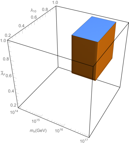
Figure 2: Allowed region in the $m_{h}$, $\bar{\lambda}_{F}$ and $\lambda_{10}$ parameter space for which $\langle h\rangle\sim 10^{16}$ GeV and the system is in its true minimum. Quantitatively, we have $3.89\times 10^{15}\leq m_{h}\leq 3.89\times 10^{16}$ GeV, $0.56\leq\bar{\lambda}_{F}$, $\lambda_{10}\leq 4\pi$, where the upper bound on $\bar{\lambda}_{F}$ and $\lambda_{10}$ results from the perturbativity limit.

We end up with three relevant free parameters in this model, namely $m_{h}$, $\bar{\lambda}_{F}$ and $\lambda_{10}$. Fig. 2 shows the allowed region in these parameters. For this plot, we imposed the requirements that the system is in the true minimum and that the minimum is stable. We demand also $\langle h\rangle\sim 10^{16}$ GeV, as required by unification. As expected, we need high values of $m_{h}$, close to the GUT scale, since $m_{h}$ is the parameter which determines the vev of $h$ via (21). Additionally, we need large values of $\bar{\lambda}_{F}$ and $\lambda_{10}$ $\in(0.5,4\pi)$, below the perturbativity limit.

Throughout this section we have found that, in order to realise a sneutrino inflation model, one needs to make some specific choices for the model parameters. As can be seen in Figs. 1 and 2, the couplings in the scalar potential (6) cannot take arbitrary values, but are constrained by the inflationary observables and the requirement of spontaneous symmetry breaking.

2.2 Singlet Inflation

Although sneutrino inflation [40, 41, 42, 43, 44, 45, 46, 47, 48] is highly appealing, it is not the only possibility for GUT inflation in the flipped SU(5)$\times$U(1) framework. The other candidate for the inflaton in the superpotential (2) is the singlet $\hat{1}_{S}$, which we study in this Section.

Focusing on the terms in the superpotential (2) that involve this singlet candidate inflaton, $\varphi=\hat{1}_{S}$, and the SU(5)$\times$U(1) breaking fields, $\nu^{c}_{H}\in\hat{10}_{H}$ and $\bar{\nu}^{c}_{H}\in\hat{\bar{10}}_{H}$, we find

$$W(\varphi,h,\bar{h})=M_{S}^{2}~{}\varphi-\mu_{S}~{}\varphi^{2}+\lambda_{S}~{}\varphi^{3}-2\lambda_{10}~{}h\bar{h}\varphi+2\mu_{10}~{}h\bar{h}\,.$$ (22)

We see that the superpotential contains terms linear, quadratic and cubic in the inflaton field $\varphi$. It is often the case that higher-order contributions to the inflationary potential, e.g. cubic and quartic terms, lead to higher values of the tensor-to-scalar ratio $r$ [9]. However, with a suitable combination of potential terms it is also possible to obtain generic values of $r$ that are lower than in quadratic inflation, as discussed in the context of the Wess-Zumino model in [50]. However, in the present work we focus on quadratic inflation only, and thus we set $\lambda_{S}=0$ in the superpotential. The $F$-term scalar potential then becomes

$$V_{F}=~{} M_{S}^{4}+4\mu_{10}^{2}(h^{2}+\bar{h}^{2})-4\lambda_{10}^{2}h^{2}\bar{h}^{2}-4\lambda_{10}M_{S}^{2}h\bar{h}$$

$$-8\lambda_{10}\mu_{10}(h^{2}+\bar{h}^{2})\varphi+8\lambda_{10}\mu_{S}h\bar{h}\varphi+4\lambda_{10}^{2}(h^{2}+\bar{h}^{2})\varphi$$

$$-4\mu_{S}M_{S}^{2}\varphi+4\mu_{S}^{2}\varphi^{2}\,.$$ (23)

Since $\varphi$ is a singlet, its potential has no $D$-terms, and the only relevant $D$-terms in (7) are those for $h$ and $\bar{h}$. As in the case of sneutrino inflation, symmetry breaking is triggered with the help of the SSB masses $m_{h}$ and $m_{\bar{h}}$ in (8).

During inflation, $h=\bar{h}=0$ is a stable minimum and the potential reduces to the simple form

$$V_{\varphi}=\left(M^{2}_{S}+2\mu_{S}\varphi\right)^{2}.$$ (24)

We perform an analysis of this singlet inflation model that is similar to the previous neutrino case, using the parameters in (10) - (LABEL:efoldings) and the values of the inflationary observables given in Table 1. The following expressions for the number of efoldings in dependence of the observables can be derived

$$N_{e}^{A_{s}} =\frac{1}{4}\sqrt{\frac{12M^{2}_{\mathrm{P}}\pi^{2}A_{s}^{\mathrm{obs}}}{\mu^{2}_{S}}}-\frac{M_{S}^{4}}{16M^{2}_{\mathrm{P}}\mu_{S}^{2}},$$

$$N_{e}^{r} >\frac{8}{r_{\mathrm{obs}}}-\frac{M_{S}^{4}}{16M^{2}_{\mathrm{P}}\mu^{2}_{S}r_{\mathrm{obs}}},$$ (25)

$$N_{e}^{n_{s}} =\frac{2}{1-n_{s}^{\mathrm{obs}}}-\frac{M_{S}^{4}}{16M^{2}_{\mathrm{P}}\mu_{S}^{2}}.$$

We present the corresponding results for different numbers of e-foldings $N_{e}=40,50,60$ in Fig. 3.

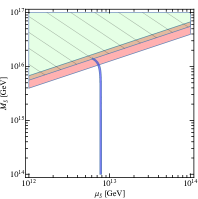
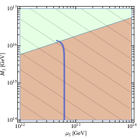
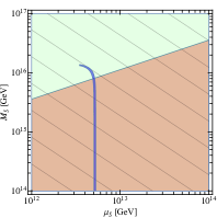
Figure 3: The $(\mu_{S},M_{S})$ planes for $N_{e}=40$ e-foldings (left panel), $N_{e}=50$ (central panel) and $N_{e}=60$ (right panel). In each case, the blue strip is compatible with the experimental value of the scalar amplitude $A_{s}$, the green shading indicates the region with an experimentally favoured value of the tensor-to-scalar ratio: $r<0.16$, and red shading indicates the region compatible with the experimental interval for the spectral tilt $n_{s}$.

As could be expected, the plots in Fig. 3 show that the scalar amplitude sets a stronger, but complementary, constraint on the parameter space compared to the effect of the other two constraints, as in the sneutrino case explored in Section 2.1. For $N_{e}=40$, only a small region of parameter space is compatible with the observables, and this could disappear entirely with a stronger upper limit on $r$. For $N_{e}=50$, however, the parameter space becomes less constrained since the bounds on $n_{s}$ and $r$ are less restrictive for a larger number of e-foldings. For $N_{e}=60$, the upper limit of the overlap region shifts slightly to smaller values of $M_{S}$. We find no lower limit for $M_{S}$, and one could take $M_{S}=0$ for a large number of e-foldings without disturbing the predictions for the observables. In that case, the result is very similar to Fig. 1 in Section 2.1, as for $M_{S}=0$ the Eqs. (2.2) reduce to Eqs. (15) of the previously studied sneutrino case. For numbers of e-foldings $N_{e}\gtrsim 50$, the predicted value of $\mu_{S}$ does not vary significantly over a large range of smaller values of $M_{S}\geq 0$.

In order to study a specific scenario with characteristics that are complementary to the scenario explored in Section 2.1, we choose for further discussion the reference point whose parameters are listed in Table 3, with $N_{e}=50$ and $M_{S}=6.03\times 10^{15}$ GeV, close to the GUT scale.

$N_{e}$	$\mu_{S}$ (GeV)	$M_{S}$ (GeV)	$\varphi^{*}$ (GeV)	$A_{s}$	$n_{s}$	$r$
50	$6.17\times 10^{12}$	$6.03\times 10^{15}$	$3.16\times 10^{19}$	$2.20\times 10^{-9}$	0.9603	0.159

Table 3: Sample scenario taken from the allowed region in Figure 3 for $N_{e}=50$.

The end of inflation is determined when $h$ and $\bar{h}$ become unstable at $h=\bar{h}=0$, which happens when

$$\varphi_{c}=\frac{\tfrac{1}{2}m_{h}-\mu_{10}}{2\lambda_{10}},\quad\varphi_{c}=\frac{\tfrac{1}{2}m_{\bar{h}}-\mu_{10}}{2\lambda_{10}}.$$ (28)

We assume for simplicity that $m_{\bar{h}}=m_{h}$, so that $h$ and $\bar{h}$ move simultaneously away from the origin and to the true minimum, breaking SU(5)$\times$U(1). With this choice, the evolutions of $h$ and $\bar{h}$ are identical, and we may assume that they take similar vevs.

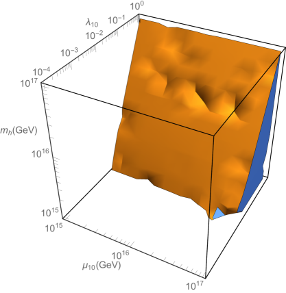
Figure 4: Region of the $(\mu_{10},\lambda_{10},m_{h})$ parameter space that allows vevs for $h$ and $\bar{h}$: $\langle h\rangle=\langle\bar{h}\rangle\sim 10^{16}$ GeV.

In this case, the inflaton $\varphi$ is free to acquire an expectation value, as it no longer violates lepton number, not being the right-handed sneutrino. Therefore, we are able to analyse the remaining parameters $m_{h}$, $\mu_{10}$ and $\lambda_{10}$ by requiring that $h$ and $\bar{h}$ acquire a vev at the GUT scale, $\langle h\rangle\sim\langle\bar{h}\rangle\sim 10^{16}$ GeV. We show in Fig. 4 the corresponding parameter space, requiring that the system falls to the true minimum.

As in the previous neutrino Section, we conclude that it is indeed possible to build a successful model for singlet inflation within flipped SU(5)$\times$U(1), if the parameters take values in the specific ranges shown in Figs. 3 and 4 so as to satisfy the experimental and theoretical constraints.

3 Embedding in SO(10)

In the previous Section we described two models of hybrid inflation within the flipped SU(5)$\times$U(1) GUT group. The superpotentials that we considered for both models are

$$W_{\phi\in\hat{10}_{F}} =\mu_{F}(\hat{10}_{F}\hat{\bar{10}}_{H}+\hat{\bar{10}}_{F}\hat{10}_{H})+\bar{\lambda}_{F}\hat{\bar{10}}_{F}\hat{10}_{H}\hat{1}_{S}+\lambda_{10}\hat{10}_{H}\hat{\bar{10}}_{H}\hat{1}_{S},$$

$$W_{\varphi\in\hat{1}_{S}} =M_{S}^{2}~{}\hat{1}_{S}+\mu_{S}\hat{1}_{S}\hat{1}_{S}+\mu_{10}\hat{10}_{H}\hat{\bar{10}}_{H}+\lambda_{10}\hat{10}_{H}\hat{\bar{10}}_{H}\hat{1}_{S}\,.$$ (29)

Both cases contain dimensionful parameters, namely $\mu_{F}$ in the scenario of sneutrino inflation and $\mu_{S}$ and $\mu_{10}$ for the singlet case. We constrained their values either by matching the inflationary observables, or by requiring symmetry breaking and a suitable true minimum for the scalar potential. However, we recall that the only real scale in the model, prior to SU(5)$\times$U(1) symmetry breaking, is the Planck scale .

One may postulate a pre-inflationary era during which a larger (semisimple?) group breaks down to SU(5)$\times$U(1), in which case the dimensionful parameters may be obtained via the expectation values of the scalar fields breaking the larger symmetry. The simplest and most straightforward case would be the group SO(10), in which SU(5)$\times$U(1) can be embedded as a maximal subgroup. In this case, all the 10-dimensional SU(5) representations can be embedded into 16-dimensional representations of SO(10). The singlet, on the other hand, can be taken either as a singlet of SO(10) or as a component of the adjoint 45-dimensional representation of SO(10). Here we choose it to be in the adjoint representation, $\hat{45}_{H}$, which we use to break SO(10) $\to$ SU(5)$\times$U(1). The SO(10) equivalents of the superpotentials in (29) are the following:

$$W_{\phi\in\hat{16}_{F}} =\lambda_{45}(\hat{16}_{F}\hat{\bar{16}}_{H}+\hat{\bar{16}}_{F}\hat{16}_{H})\hat{45}_{H}+\bar{\lambda}_{F}\hat{\bar{16}}_{F}\hat{16}_{H}\hat{45}_{H}+\lambda_{10}\hat{16}_{H}\hat{\bar{16}}_{H}\hat{45}_{H},$$

$$W_{\varphi\in\hat{1}_{S}}$$

for the two possible assignments of the SU(5) singlet field, as indicated.

The SO(10) symmetry is broken when $\hat{45}_{H}$ acquires a vev in its SU(5)$\times$U(1) singlet direction: $\langle\hat{45}_{H}\rangle=v$. The SO(10) representations are then broken, and give rise to (among others) the terms in (29). In both cases, we make the following identifications:

$$\mu_{F} =v\lambda_{45},$$

$$M_{S}^{2} =v^{2}\lambda_{45},\quad\mu_{S}=v\lambda_{45},\quad\mu_{10}=v\lambda_{45}^{\prime}.$$ (30)

Considering now the reference points shown in Tables 2 and 3, for which $\mu_{F}\sim\mu_{S}\lesssim 10^{13}$ GeV, we can fix the values of the couplings of the SO(10) model. Assuming that SO(10) breaking happens above the GUT scale, $v\gtrsim 10^{16}$ GeV, we find that $\lambda_{45}\lesssim 10^{-3}$. This is consistent with the fact that we have taken $M_{S}\neq 0$ in Section 2.2, as we find now that $M_{S}=v\sqrt{\lambda_{45}}\sim 10^{15}$ GeV, which roughly matches and motivates our choice in Table 3.

Although this embedding into SO(10) seems reasonable and provides a suitable superpotential prior to inflation, it looses the ultraviolet connection with weakly-coupled string theory. This is because it is, in general, not possible to obtain such large representations as $\hat{45}_{H}$ from a manifold compactification of string theory [38, 39]. One possible alternative would be to consider flipped SO(10)$\times$U(1) as the pre-inflationary GUT symmetry group . This differs from the usual SO(10) in that the SM matter content is not fully embedded in a 16-dimensional representation, but in the direct sum $16_{1}\oplus 10_{-2}\oplus 1_{4}$. This kind of model could in principle be derived from string compactification, since it no longer requires large field representations: the symmetry breaking SO(10)$\times$U(1) $\to$ SU(5)$\times$U(1) can be realised by a pair of representations $16_{1}\oplus\bar{16}_{-1}$. However, the only way to obtain superpotentials such as (29) would be with non-renormalisable terms involving four 16-dimensional representations.

Thus, the embedding of the flipped SU(5)$\times$U(1) inflationary model into SO(10) can in principle be realised at least in two ways, but both of them require forsaking some of the advantages of the original flipped SU(5)$\times$U(1) model. Embeddings into larger groups such as E₆ or E₈ might be also possible, but lie beyond the scope of this work.

4 Discussion and Outlook

We have discussed in this work various scenarios for GUT inflation. Motivated by its lack of magnetic monopoles and its possible connection with string theory, we first considered the flipped SU(5)$\times$U(1) gauge group. We explored two scenarios, in which the inflaton is identified with a sneutrino field, and another in which the inflaton is a gauge singlet. The neutrino option is attractive because of its possible closer connection with observables in low-energy physics, whereas the singlet option has more flexibility. As we have also discussed, both of these scenarios may be embedded within larger GUT groups that are broken before inflation. The simplest option is SO(10), but in this case the link to weakly-coupled string theory is lost. As a more string-compatible option, we have also considered embedding flipped SU(5)$\times$U(1) in flipped SO(10)$\times$U(1).

We consider the studies in this paper to be exploratory, in the sense that we have not investigated all the potential issues in such models. For example, we have considered simple cases in which two- or multi-field effects can be neglected, and it would be interesting to consider more general cases whose potentials could be more flexible. Also, we have used a specific assumption on the scale of soft SUSY breaking that could be questioned. Indeed, there is as yet no consensus how and at what scale SUSY is broken, so it would be interesting to explore alternative scenarios.

Whilst acknowledging these limitations in our study, we think that the models explored in this paper furnish interesting existence proofs for GUT inflation, and that they offer intriguing perspectives for possible future studies.

References

- [1] J. R. Ellis, S. Kelley, and D. V. Nanopoulos, Phys.Lett. B260, 131 (1991).
- [2] U. Amaldi, W. de Boer, and H. Furstenau, Phys.Lett. B260, 447 (1991).
- [3] P. Langacker and M.-x. Luo, Phys.Rev. D44, 817 (1991).
- [4] C. Giunti, C. Kim, and U. Lee, Mod.Phys.Lett. A6, 1745 (1991).
- [5] Planck Collaboration, P. Ade et al., Astron.Astrophys. 571, A22 (2014), 1303.5082.
- [6] A. A. Starobinsky, Phys.Lett. B91, 99 (1980).
- [7] BICEP2 Collaboration, P. Ade et al., Phys.Rev.Lett. 112, 241101 (2014), 1403.3985.
- [8] Planck Collaboration, R. Adam et al., (2014), 1409.5738.
- [9] M. P. Hertzberg and F. Wilczek, (2014), 1407.6010.
- [10] A. D. Linde, Phys.Lett. B259, 38 (1991).
- [11] A. R. Liddle and D. H. Lyth, Phys.Rept. 231, 1 (1993), astro-ph/9303019.
- [12] A. D. Linde, Phys.Rev. D49, 748 (1994), astro-ph/9307002.
- [13] E. J. Copeland, A. R. Liddle, D. H. Lyth, E. D. Stewart, and D. Wands, Phys.Rev. D49, 6410 (1994), astro-ph/9401011.
- [14] E. D. Stewart, Phys.Lett. B345, 414 (1995), astro-ph/9407040.
- [15] L. Randall, M. Soljacic, and A. H. Guth, Nucl.Phys. B472, 377 (1996), hep-ph/9512439.
- [16] L. Randall, M. Soljacic, and A. H. Guth, (1996), hep-ph/9601296.
- [17] J. Garcia-Bellido, A. D. Linde, and D. Wands, Phys.Rev. D54, 6040 (1996), astro-ph/9605094.
- [18] D. H. Lyth, JCAP 1205, 022 (2012), 1201.4312.
- [19] A. H. Guth and E. I. Sfakianakis, (2012), 1210.8128.
- [20] F. Brummer, V. Domcke and V. Sanz, JCAP08 (2014) 066, hep-ph/1405.4868.
- [21] A. B. Lahanas and D. V. Nanopoulos, Phys. Rept. 145 (1987) 1.
- [22] M. Kawasaki, M. Yamaguchi and T. Yanagida, Phys. Rev. Lett. 85 (2000) 3572, hep-ph/0004243.
- [23] H. Georgi and S. Glashow, Phys.Rev.Lett. 32, 438 (1974).
- [24] G. ’t Hooft, Nucl.Phys. B79, 276 (1974).
- [25] A. M. Polyakov, JETP Lett. 20, 194 (1974).
- [26] A. H. Guth, Phys.Rev. D23, 347 (1981).
- [27] A. De Rujula, H. Georgi, and S. Glashow, Phys.Rev.Lett. 45, 413 (1980).
- [28] S. M. Barr, Phys.Lett. B112, 219 (1982).
- [29] J. P. Derendinger, J. E. Kim and D. V. Nanopoulos, Phys. Lett. B 139 (1984) 170.
- [30] I. Antoniadis, J. R. Ellis, J. Hagelin, and D. V. Nanopoulos, Phys.Lett. B194, 231 (1987).
- [31] J. R. Ellis, J. Hagelin, S. Kelley, and D. V. Nanopoulos, Nucl.Phys. B311, 1 (1988).
- [32] T. Li, J. A. Maxin, D. V. Nanopoulos, and J. W. Walker, J.Phys. G40, 115002 (2013), 1305.1846.
- [33] J. L. Lopez and D. V. Nanopoulos, (1997), hep-ph/9701264.
- [34] B. Campbell, J. R. Ellis, J. Hagelin, D. V. Nanopoulos, and R. Ticciati, Phys.Lett. B198, 200 (1987).
- [35] I. Antoniadis, J. R. Ellis, J. Hagelin, and D. V. Nanopoulos, Phys.Lett. B205, 459 (1988).
- [36] I. Antoniadis, J. R. Ellis, J. S. Hagelin, and D. V. Nanopoulos, Phys.Lett. B208, 209 (1988).
- [37] I. Antoniadis, J. R. Ellis, J. Hagelin, and D. V. Nanopoulos, Phys.Lett. B231, 65 (1989).
- [38] H. P. Nilles, Phys.Rept. 110, 1 (1984).
- [39] A. Brignole, L. E. Ibanez, and C. Munoz, Adv.Ser.Direct.High Energy Phys. 21, 244 (2010), hep-ph/9707209.
- [40] H. Murayama, H. Suzuki, T. Yanagida, and J. Yokoyama, Phys.Rev.Lett. 70, 1912 (1993).
- [41] J. R. Ellis, M. Raidal, and T. Yanagida, Phys.Lett. B581, 9 (2004), hep-ph/0303242.
- [42] S. Antusch, M. Bastero-Gil, S. F. King, and Q. Shafi, Phys.Rev. D71, 083519 (2005), hep-ph/0411298.
- [43] C.-M. Lin and J. McDonald, Phys.Rev. D74, 063510 (2006), hep-ph/0604245.
- [44] F. Deppisch and A. Pilaftsis, JHEP 0810, 080 (2008), 0808.0490.
- [45] S. Antusch et al., JHEP 1008, 100 (2010), 1003.3233.
- [46] S. Antusch, J. P. Baumann, V. F. Domcke, and P. M. Kostka, JCAP 1010, 006 (2010), 1007.0708.
- [47] J. Ellis, M. Fairbairn, and M. Sueiro, JCAP 1402, 044 (2014), 1312.1353.
- [48] H. Murayama, K. Nakayama, F. Takahashi, and T. T. Yanagida, Phys.Lett. B738, 196 (2014), 1404.3857.
- [49] J. Ellis, D. V. Nanopoulos and K. A. Olive, Phys. Rev. D 89 (2014) 4, 043502, [arXiv:1310.4770 [hep-ph]].
- [50] D. Croon, J. Ellis, and N. E. Mavromatos, Phys.Lett. B724, 165 (2013), 1303.6253.
- [51] A. R. Liddle, P. Parsons, and J. D. Barrow, Phys.Rev. D50, 7222 (1994), astro-ph/9408015.
- [52] D. Baumann, (2009), 0907.5424.
- [53] J. Martin, C. Ringeval, and V. Vennin, Phys.Dark Univ. (2014), 1303.3787.
- [54] F. Vernizzi and D. Wands, JCAP 0605, 019 (2006), astro-ph/0603799.
- [55] Z. Lalak, D. Langlois, S. Pokorski, and K. Turzynski, JCAP 0707, 014 (2007), 0704.0212.
- [56] V. F. Mukhanov and P. J. Steinhardt, Phys.Lett. B422, 52 (1998), astro-ph/9710038.
- [57] C. Gordon, D. Wands, B. A. Bassett, and R. Maartens, Phys.Rev. D63, 023506 (2001), astro-ph/0009131.
- [58] A. A. Starobinsky, S. Tsujikawa, and J. Yokoyama, Nucl.Phys. B610, 383 (2001), astro-ph/0107555.
- [59] F. Di Marco, F. Finelli, and R. Brandenberger, Phys.Rev. D67, 063512 (2003), astro-ph/0211276.
- [60] S. Tsujikawa, D. Parkinson, and B. A. Bassett, Phys.Rev. D67, 083516 (2003), astro-ph/0210322.
- [61] F. Di Marco and F. Finelli, Phys.Rev. D71, 123502 (2005), astro-ph/0505198.
- [62] C. T. Byrnes and D. Wands, Phys.Rev. D74, 043529 (2006), astro-ph/0605679.
- [63] K.-Y. Choi, L. M. Hall, and C. van de Bruck, JCAP 0702, 029 (2007), astro-ph/0701247.
- [64] D. Langlois and S. Renaux-Petel, JCAP 0804, 017 (2008), 0801.1085.
- [65] C. M. Peterson and M. Tegmark, Phys.Rev. D83, 023522 (2011), 1005.4056.
- [66] R. Easther, J. Frazer, H. V. Peiris, and L. C. Price, Phys.Rev.Lett. 112, 161302 (2014), 1312.4035.
- [67] W. Buchmüller, V. Domcke, K. Kamada and K. Schmitz, JCAP 1407 (2014) 054, [arXiv:1404.1832 [hep-ph]] and references therein.