Topological order and the vacuum of Yang-Mills theories.

Abstract

We study, for $SU(2)$ Yang-Mills theories discretized on a lattice, a non-local topological order parameter, the center flux ${{z}}$. We show that: i) well defined topological sectors classified by $\pi_{1}(SO(3))=\mathbb{Z}_{2}$ can only exist in the ordered phase of ${{z}}$; ii) depending on the dimension $2\leq d\leq 4$ and action chosen, the center flux exhibits a critical behaviour sharing striking features with the Kosterlitz-Thouless type of transitions, although belonging to a novel universality class; iii) such critical behaviour does not depend on the temperature $T$. Yang-Mills theories can thus exist in two different continuum phases, characterized by an either topologically ordered or disordered vacuum; this reminds of a quantum phase transition, albeit controlled by the choice of symmetries and not by a physical parameter.

I Introduction

Of all ideas applied to the confinement problem in non-abelian Yang-Mills theories Jaffe and Witten (2000); Greensite (2011) the most popular still involve topological degrees of freedom of some sort Wu and Yang (1969); Nielsen and Olesen (1973); ’t Hooft (1974); Mandelstam (1975); Polyakov (1977); Goddard et al. (1977); Mandelstam (1979); Weinberg (1980); Seiberg and Witten (1994). Among these center vortices ’t Hooft (1978, 1979); Mack and Pietarinen (1982) have enjoyed broad attention, in particular in the lattice literature. Although most of the effort was put in dealing with gauge fixed schemes, some investigations actually attempted to tackle the problem in a gauge invariant way Kovacs and Tomboulis (2000); Hart et al. (2000); de Forcrand et al. (2001); de Forcrand and von Smekal (2002); Burgio et al. (2006a, 2007); von Smekal (2012) and are therefore directly related to ’t Hooft’s original idea.

Non-abelian gauge fields transform under the group’s adjoint representation, $SU(N)/\mathbb{Z}_{N}$. Such group is not simply connected, with a non trivial first homotopy class:

$$\pi_{1}(\frac{SU(N)}{\mathbb{Z}_{N}})=\mathbb{Z}_{N}\,,$$ (1)

the center of $SU(N)$. Following Ref. ’t Hooft (1979), let us consider the Euclidean Yang-Mills theory on a $d$-dimensional torus, i.e. with all directions compactified, and choose one of the $d$ Euclidean directions as time. If large gauge transformations classified by Eq. (1) induce a super-selection rule, we can decompose the physical Hilbert space ${\cal{H}}$ of gauge invariant states Burgio et al. (2000) in sub-spaces ${\cal{H}}_{\vec{k},\vec{m}}$ labeled by topological indices, the $\mathbb{Z}_{N}$ electric and magnetic fluxes (vortices) $\vec{k}=(k_{1},\ldots,k_{n_{t}})$ and $\vec{m}=(m_{1}\ldots,m_{n_{s}})$ ’t Hooft (1979):

$${\cal{H}}=\bigoplus_{{k}_{i},{m}_{j}=0}^{N-1}{\cal{H}}_{\vec{k},\vec{m}}\,.$$ (2)

Here $n_{t}=d-1$ counts the space-time and $n_{s}=\frac{(d-1)(d-2)}{2}$ the space-space planes and $k_{i},m_{i}\in\mathbb{Z}_{N}$. As ’t Hooft pointed out, a sufficient condition for confinement is realized if the low-temperature phase of pure Yang-Mills theories corresponds to a superposition of all (electric) sectors, while above the deconfinement transition such $\mathbb{Z}_{N}$ symmetry must get broken to the trivial one ’t Hooft (1978, 1979).

One can check such scenario by calculating, e.g. in lattice simulations, how the free energy for $\mathbb{Z}_{N}$ flux creation:

$$F(\vec{k})=\Delta\,{\cal{U}}_{\vec{k}}-T\,\Delta\,{\cal{S}}_{\vec{k}}=-\log{\frac{Z(\vec{k})}{Z(\vec{0})}}$$ (3)

changes with the temperature $T$ across the deconfinement transition. Here $\Delta\,{\cal{U}}_{\vec{k}}$ is the energy (action) cost to generate the $\vec{k}^{\rm{th}}$ (electric) vortex from the vacuum, $\Delta\,{\cal{S}}_{\vec{k}}$ the corresponding entropy change and $Z(\vec{k})$ the partition function restricted to the topological sector labeled by $\vec{k}$. For the one-vortex sector, $F$ is nothing but the free energy of a maximal ’t Hooft loop, giving a confinement criterion dual to Wilson’s: in the thermodynamic limit $F$ should vanish in the confined phase while it should diverge as $\tilde{\sigma}(T)\,L^{2}$ above the deconfinement temperature $T_{c}$, where $\tilde{\sigma}(T)$ is the dual string tension ’t Hooft (1979); Greensite (2011); Kovacs and Tomboulis (2000); Hart et al. (2000); de Forcrand et al. (2001); de Forcrand and von Smekal (2002); de Forcrand and Jahn (2003); Burgio et al. (2006a). In other words, a perimeter law for the Wilson loop implies an area law for the ’t Hooft loop and vice-versa ’t Hooft (1978, 1979).

Of course, when considering the theory at $T=0$, the distinction between electric and magnetic fluxes is artificial. In this case all the $N^{\frac{d(d-1)}{2}}$ topological sectors must be taken into account when establishing whether $\mathbb{Z}_{N}$-symmetry is unbroken, i.e. whether the vacuum $|\Psi_{0}\rangle$ is indeed a symmetric superposition of states belonging to ${\cal{H}}_{\vec{k},\vec{m}}$:

$$|\Psi_{0}\rangle=\sum_{\vec{k},\vec{m}}|\Psi_{0}^{\vec{k},\vec{m}}\rangle\,.$$ (4)

In the following we will use either definition, depending on whether we are considering the $T=0$ or the $T>0$ case.

The above ideas generalize naturally to the lattice discretization of Yang-Mills theories; the specific action used plays however a key role in their actual implementation. If one wishes to preserve the symmetries of the continuum theory the natural choice should fall on a discretization transforming under the “correct” group $SU(N)/\mathbb{Z}_{N}$. One possibility among many (see e.g. Ref. Halliday and Schwimmer (1981a)) is given by the adjoint Wilson action with periodic boundary conditions de Forcrand and Jahn (2003):

$$S_{A}=\beta_{A}\sum_{P}\left(1-\frac{1}{N^{2}-1}\mbox{Tr}_{A}\,U_{P}\right)\,,$$ (5)

where $U_{P}$ is the standard plaquette. For $N=2$ it was indeed shown in Refs. Burgio et al. (2006a, 2007); Barresi and Burgio (2007) that for simulations based on Eq. (5):

i) $\mathbb{Z}_{2}$ topological sectors are well defined in the continuum limit, both below and above $T_{c}$, i.e. the decomposition in Eq. (2) holds;

ii) the partition function $Z_{A}=\int\exp{(-S_{A})}$ dynamically includes all sectors;

iii) in the deconfined phase all non trivial sectors are suppressed, while as $T\to 0$ all sectors are equivalent, i.e. the vacuum can be described by Eq. (4).

The main difficulty of such setup lies of course in the implementation of an algorithm capable of tunneling ergodically among all vortex topologies. Simulations are therefore quite demanding: reaching enough statistics to check whether the symmetry among sectors postulated in Eq. (2) remains unbroken from $T=0$ all the way up to $T_{c}$ is difficult; the evidence given in Refs. Burgio et al. (2006a, 2007) seems to point to a more complicated picture.

Alternatively, universality Svetitsky and Yaffe (1982) should allow the use of the fundamental Wilson action:

$$S_{F}=\beta_{F}\sum_{P}\left(1-\frac{1}{N}\Re\left[\mbox{Tr}_{F}\,U_{P}\right]\right)\,,$$ (6)

which is the quenched (mass $\to\infty$) limit of the physical action coupling Yang-Mills theories to fundamental fermions, e.g. full QCD. In this case, however, some care must be taken in defining a $SU(N)/\mathbb{Z}_{N}$ invariant theory. Indeed, in the presence of fundamental fermions the topological classification of Eq. (1) breaks down. The extension to full QCD has been indeed one of the main obstacles in establishing the ’t Hooft vortex picture as a viable model for confinement. We will comment on this in Sec. IV; for the moment, let us note that one can still introduce vortex topological sectors “statically” by simply imposing twisted boundary conditions de Forcrand et al. (2001); de Forcrand and von Smekal (2002); de Forcrand and Jahn (2003). We should then be able to reconstruct the “full” partition function ${Z_{F}}$ by taking the weighted sum of all partition functions $Z_{F}(\vec{k},\vec{m})=\int\exp{(-S_{F}({\vec{k},\vec{m}}))}$ with boundary conditions corresponding to the sector labeled by $\vec{k}$ and $\vec{m}$ de Forcrand et al. (2001); de Forcrand and von Smekal (2002). Since each $Z_{F}(\vec{k},\vec{m})$ must be determined via independent simulations, their relative weights can only be calculated through indirect means. Still, such simulations are computationally more efficient than in the $Z_{A}$ case and have therefore been the method of choice in most investigations of Eq. (3) Kovacs and Tomboulis (2000); Hart et al. (2000); de Forcrand et al. (2001); de Forcrand and von Smekal (2002); von Smekal (2012).

Investigations using Eq. (6) rely on the assumption that fixing the boundary conditions is enough to ensure that the Hilbert-space decomposition defined in Eq. (2) works. However, it is well known that upon discretization of Yang-Mills theories $\mathbb{Z}_{N}$ magnetic monopoles are generated at strong coupling Lubkin (1963); Mack and Petkova (1979, 1982); Halliday and Schwimmer (1981b, a); Coleman (1982), causing bulk phenomena in the $\beta_{F}-\beta_{A}$ phase diagram. Now, since the $\mathbb{Z}_{N}$ fluxes defining our topological sectors live on the co-set of a two dimensional plane, they have a simple geometrical interpretation: they are described in $d=4$ by a closed world-sheet, i.e. they are string-like objects, and in $d=3$ by a closed world-line, i.e. particle-like. On the other hand, topological lattice artifacts as the above mentioned $\mathbb{Z}_{N}$ monopoles are themselves sources of $\mathbb{Z}_{N}$ flux: in $d=4$ they will be particle-like objects, their closed world-lines bounding open $\mathbb{Z}_{N}$ flux world-sheets, while in $d=3$ they will be instanton-like objects and will be end-points of open $\mathbb{Z}_{N}$ flux lines Lubkin (1963); Mack and Petkova (1979, 1982); Coleman (1982); de Forcrand and Jahn (2003). $\mathbb{Z}_{N}$ monopoles are therefore in one to one correspondence with open center vortices; in other words, universality between the fundamental and adjoint actions can only be invoked when just closed, i.e. truly topological ${\mathbb{Z}}_{N}$ vortices winding around the compactified directions can form. Notice how in $d=2$, where no $\mathbb{Z}_{N}$ monopoles can exist, $\mathbb{Z}_{N}$ fluxes are instanton type objects. The distinction between open and closed vortices is in this case blurred, but in a non-ergodic setup it can eventually be made through the flux allowed by the boundary conditions chosen.

The above discussion has a straightforward consequence. If one could “measure” whether open ${\mathbb{Z}}_{N}$ vortices are absent in a given discretization, i.e. whether only topological vortices can be generated from the vacuum, there would be no need to monitor $\mathbb{Z}_{N}$ monopoles to establish universality between $S_{A}$ and $S_{F}$ in the first place, since these must be absent anyway. This would have two advantages: first, such criterion could be generalized to $d=2$. Second, absence of lattice artifacts, whether for $S_{F}$, for $S_{A}$ or for both, would get “promoted” to a necessary condition for the super-selection rule of Eq. (2), and hence for the conjectured vacuum symmetry of Eq. (4), to be realized. Indeed, consider states belonging to distinct topological sectors labeled by the indices $k$, $k^{\prime}\in\mathbb{Z}_{N}$.

Figure 1: Illustration of the ambiguity in labeling the ${\mathbb{Z}}_{N}$ topological sectors in presence of open vortices. Should the given configuration (top) be counted to the $k^{\mathrm{th}}$ (middle) or to the $k^{\prime\mathrm{th}}$ (bottom) sector?

The presence of open vortices immediately blurs the distinction among them: does the state pictured at the top of Fig. 1 belong to the $k^{\mathrm{th}}$ sector, resulting from the superposition of $k$ closed vortices with ${\mathrm{mod}}(k^{\prime}-k)_{N}$ open ones (middle picture), or does it belong to the $k^{\prime\mathrm{th}}$ sector, coming from the superposition of $k^{\prime}$ closed vortices with ${\mathrm{mod}}(k-k^{\prime})_{N}$ open ones winding in the other direction (bottom picture)? Clearly, there is no way to distinguish between them and assign the configuration to $Z(k)$ rather than $Z(k^{\prime})$ in Eq. (3). In other words, a Wilson loop will never know if the vortex piercing it to generate the area law for its expectation value ’t Hooft (1978, 1979) is open or closed: a confinement criterion based on the vortex free energy $F$ and hence on the ’t Hooft loop can only make sense if open vortices are absent at any temperature.

In this paper we will investigate a topological order parameter, the center flux ${{z}}$, for the transition between phases characterized by the presence of open or closed $\mathbb{Z}_{2}$ vortices in $SU(2)$ Yang-Mills theories at $T=0$, discretized through standard plaquette actions. We will show that, depending on the action, the dimensions and the volume, the theory can be either in a topologically ordered or disordered phase; such distinction will persist at finite $T$. In the disordered phase open vortices dominate the vacuum and $\mathbb{Z}_{2}$ topological sectors are ill defined; the Hilbert space of Yang-Mills theories cannot be classified by a super-selection as in Eq. (2). Such disordered phase is compatible with the presence of fundamental fermions; the ordered phase, on the other hand, should be the correct one when coupling $SU(2)$ with adjoint fermions, a popular candidate for infrared conformal gauge theories.

Besides this (perhaps lengthy) introduction, the rest of the paper is organized as follows: Sec. II contains details on the lattice setup, observables and simulation techniques; in Sec. III the main results will be presented; Sec. IV contains the conclusions and outlook. Preliminary results of this investigations have been presented in Refs. Burgio (2007, 2014).

II Setup

II.1 Action and Observables

We will consider the $SU(2)$ mixed fundamental-adjoint Wilson action with periodic boundary conditions in $2\leq d\leq 4$ Euclidean dimensions, as given in Eqs. (5, 6):

$$S = \beta_{A}\sum_{P}\left(1-\frac{1}{3}\mbox{Tr}_{A}\,U_{P}\right)+\beta_{F}\sum_{P}\left(1-\frac{1}{2}\mbox{Tr}_{F}\,U_{P}\right)$$

$$\frac{1}{a^{4-d}\,g^{2}} = \frac{1}{4}\beta_{F}+\frac{2}{3}\beta_{A}\,,$$ (7)

where $a$ is the (dimensionful) lattice spacing and $U_{P}$ denotes the $1\times 1$ plaquette; all results can be easily generalized to different boundary conditions. For higher groups $SU(N)$ the general picture should not change dramatically Creutz and Moriarty (1982a, b); Drouffe et al. (1982); Ardill et al. (1983, 1984); Barresi and Burgio (2007). However, other representations than just the fundamental and adjoint are allowed. Many details might therefore depend on $N$; direct investigations of at least the $SU(3)$ case would be welcome.

In $d\geq 3$, $\mathbb{Z}_{2}$ monopoles can be defined for each elementary cube $c$ through the product:

$$\sigma_{c}=\prod_{{P}\in\partial c}\mathrm{sign}(\mbox{Tr}_{F}\,U_{{P}})\,,$$ (8)

over all plaquettes $U_{{P}}$ belonging to its surface $\partial c$ Halliday and Schwimmer (1981b, a); de Forcrand and Jahn (2003); Barresi et al. (2004a); Barresi and Burgio (2007). Notice how rescaling any link by a $\mathbb{Z}_{2}$ factor will leave $\sigma_{c}$ unchanged.

The $\mathbb{Z}_{2}$ monopole density should vanish in the continuum limit $g^{2}\to 0$. This happens, however, in different ways, depending on the dimensions $d$ or the direction along which such limit is taken in the $\beta_{F}-\beta_{A}$ plane, and has been the subject of intense investigations in the pioneering years of lattice gauge theories Drouffe and Zuber (1981); Greensite and Lautrup (1981); Bhanot and Creutz (1981); Halliday and Schwimmer (1981b); Creutz and Moriarty (1982a, b); Drouffe et al. (1982); Ardill et al. (1983, 1984); Baig and Cuervo (1987a, b, 1988); Bursa and Teper (2006). For the $SU(2)-SO(3)$ case considered here the resulting phase diagrams in $d=3$ and 4 are sketched in Figs. 2, 3;

Figure 2: Phase diagram of the fundamental-adjoint plane for $d=3$. Continuous lines indicate bulk transitions, dashed lines the roughening transition, dotted lines the crossover regions associated with $\mathbb{Z}_{2}$ monopoles. Similar diagrams hold for higher $N$.

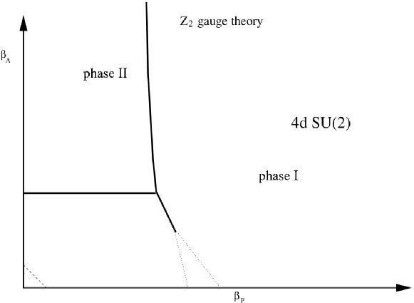
Figure 3: Phase diagram of the fundamental-adjoint plane for $d=4$. Continuous lines indicate bulk transitions, dashed lines the roughening transition, dotted lines the crossover regions associated with $\mathbb{Z}_{2}$ monopoles. Similar diagrams hold for higher $N$.

similar ones have been established for $N\geq 3$, see e.g. Refs. Creutz and Moriarty (1982a, b); Drouffe et al. (1982); Ardill et al. (1983, 1984). Continuous lines indicate bulk transitions Greensite and Lautrup (1981); Bhanot and Creutz (1981); Halliday and Schwimmer (1981b); Baig and Cuervo (1987b), dashed lines the roughening transition Drouffe and Zuber (1981), dotted lines the crossover regions associated with $\mathbb{Z}_{2}$ monopoles Halliday and Schwimmer (1981b); Baig and Cuervo (1987b). The vertical bulk transition line coming down form $\beta_{A}=\infty$ corresponds to the underlying $\mathbb{Z}_{2}$ gauge theory: in $d=3$ it ends at a finite point Baig and Cuervo (1987b, 1988); Bursa and Teper (2006), while in $d=4$ it joins the bulk transition line associated with $\mathbb{Z}_{2}$ monopoles Greensite and Lautrup (1981); Bhanot and Creutz (1981); Halliday and Schwimmer (1981b); from the endpoint of the latter a crossover region starts, extending beyond the $\beta_{F}$ axis. In $d=2$, $\mathbb{Z}_{2}$ monopoles are of course absent. Furthermore, the $\mathbb{Z}_{2}$ gauge theory has no phase transition; apart from the roughening transition Drouffe and Zuber (1981), the corresponding phase diagram should therefore be free of any bulk effects, including crossovers.

From Fig. 3 it is obvious that two distinct continuum limits in $d=4$ exist, depending if $g^{2}\to 0$ in Eq. (7) is taken within Phase I or II. Phase II at fixed twist has been shown in Refs. de Forcrand and Jahn (2003); Barresi and Burgio (2007) to be equivalent to a positive plaquette model Mack and Pietarinen (1982); Bornyakov et al. (1991); Fingberg et al. (1995) with fixed twisted boundary conditions. Although such model and the fundamental Wilson action seem to describe the same physics, the two phases are always separated by a bulk transition line. What is thus the difference, if any, between them?

A first hint towards an explanation to this (long neglected) puzzle is given by the results of Refs. Burgio et al. (2006a, 2007); Barresi et al. (2002, 2003a, 2004a, 2003b, 2004b, 2004c); Burgio et al. (2006b); Barresi and Burgio (2007): in the continuum limit the $d=4$ adjoint theory ($\beta_{F}\equiv 0$), which lies precisely within phase II, possesses well defined $\mathbb{Z}_{2}$ topological sectors, i.e. no open vortices: the Hilbert-space decomposition defined in Eq. (2) works! On the other hand, one can easily check that in phase I, across all crossovers, the $\mathbb{Z}_{2}$ monopole density vanishes quite slowly as $g^{2}\to 0$: their persistence in the weak coupling phase should reflect itself in the presence of open $\mathbb{Z}_{2}$ vortices, possibly spoiling Eq. (2). Could the difference between phase I and II lie in whether such super-selection rule is indeed realized for the Hilbert space of Yang-Mills theories? To find out, we can start from the twist operator, which “counts” the $\mathbb{Z}_{2}$ vortices piercing all parallel planes for a fixed choice of $\mu$-$\nu$ ’t Hooft (1979); de Forcrand and Jahn (2003):

$$z_{\mu\nu}=\frac{1}{L^{d-2}}\,\sum_{\hat{y}\,\bot\,{\mu\nu}-{\rm plane}}\;\prod_{\hat{x}\,\in\,{\mu\nu}-{\rm plane}}\mathrm{sign}({\mbox{Tr}}_{F}U_{\mu\nu}(\hat{x},\hat{y}))\,.$$ (9)

$U_{\mu\nu}$ and $\hat{x}$, respectively, denote a $1\times 1$ plaquette and point lying in the $\mu$-$\nu$ plane, while $\hat{y}$ denotes a point on its co-set, which is obviously empty in $d=2$; only a single plane contributes to the sum in this case. Notice how $z_{\mu\nu}$, like $\sigma_{c}$, is unaffected by any multiplication of links by a center element, i.e. it is insensitive to the spurious $\mathbb{Z}_{2}$ gauge degrees of freedom.

If topological sectors are well defined, all parallel planes will contribute with the same sign to the sum in Eq. (9). For any fixed $\mu$ and $\nu$, $z_{\mu\nu}$ can thus only take the values $\pm 1$, depending on the boundary conditions chosen. E.g., for the periodic boundary conditions considered in this paper, the topological sector must always be trivial: $z_{\mu\nu}\equiv 1$ $\forall\mu,\nu$. When, however, topological sectors are ill defined the contributions to the sum in Eq. (9) can change from plane to plane; in particular, if open $\mathbb{Z}_{2}$ vortices pierce the planes randomly, all $z_{\mu\nu}$ will average to zero. To make such statement quantitative and characterize how the transition from the disordered to the ordered regime takes place we define a (non-local!) order parameter, the center flux ${{z}}$, such that its expectation value $\langle{{z}}\rangle\equiv 1$ if, whatever the boundary conditions, vortex topology takes the correct value expected from the super-selection rule, while $\langle{{z}}\rangle\equiv 0$ when $\mathbb{Z}_{2}$ fluxes are maximally randomized. For $d\geq 3$:

$${{z}}=\frac{2}{d(d-1)}\sum_{\mu>\nu=1}^{d}|z_{\mu\nu}|\,,$$ (10)

while for $d=2$, since $|z_{12}|\equiv 1$, we will define:

$${{z}}=1-|z_{12}-\langle z_{12}\rangle|\,.$$ (11)

Notice that the latter definition will only work as long as $\beta_{F}\neq 0$, i.e. when the $d=2$ theory cannot tunnel among topological sectors. In the following we will investigate, either analytically (in $d=2$) or via Monte-Carlo simulations (for $d\geq 3$), the behaviour of the center flux and its susceptibility:

$$\chi_{{z}}=L^{d}\,\;\left({{z}}-\langle{{z}}\rangle\right)^{2}\,.$$ (12)

II.2 Algorithm

Simulations for $\beta_{A}=0$, i.e. along the $\beta_{F}$ axis, have been performed using a standard heat-bath algorithm followed by micro-canonical steps. Although this cannot be extended to $\beta_{A}\neq 0$, as long as also $\beta_{F}\neq 0$ one can use the biased Metropolis $+$ micro-canonical algorithm introduced in Refs. Bazavov and Berg (2005); Bazavov et al. (2005). The lookup tables for the pseudo-heat-bath probability need to be fixed beforehand: sizes between $32\times 32$ and $64\times 64$ were found to be sufficient Bazavov and Berg (2005); Bazavov et al. (2005). As long as $\beta_{F}\gg\beta_{A}$, the algorithm is for all practical purposes just as efficient as an heat-bath, as the amount of accepted proposals stays well above $95\%$. On the other hand, whenever $\beta_{F}\ll\beta_{A}$ the rejected pseudo-heat-bath and micro-canonical updates increase considerably. This becomes a real issue when simulating around the peaks of the susceptibility Eq. (12), where auto-correlations for ${{z}}$ and $\chi_{{z}}$ become quite large. One can try to combat such critical slowing down, unavoidable when dealing with any phase transition, by increasing the number of micro-canonical steps per biased Metropolis update. Unfortunately this turns out to be less efficient than for the $\beta_{F}\gtrsim\beta_{A}$ case or for the heat-bath algorithm; only with runs of order $\sim 10^{8}$ sweeps one eventually reaches a good signal-to-noise ratio for $\chi_{{z}}$. Since the $d=3$ case will anyway turn out to be the most interesting from the point of view of the critical behaviour, while in $d=2$ analytic results allow to gain otherwise control of the problem, we have limited a precise finite size scaling (FSS) Fisher and Barber (1972) analysis to determine the properties of the transition to the $\beta_{A}=0$, $d=3$ case. Still, we have performed simulations for a whole range of parameters and lattice sizes $L$ in $2\leq d\leq 4$, trying to explore the whole $\beta_{F}-\beta_{A}$ plane. We have nevertheless avoided phase II of the $d=4$ phase diagram in Fig. 3, since it would have called for completely different simulation techniques; see Refs. Burgio et al. (2006a, 2007); Barresi et al. (2002, 2003a, 2004a, 2003b, 2004b, 2004c); Burgio et al. (2006b); Barresi and Burgio (2007) for results in this parameter region.

III Results

III.1 $d=2$

The $SU(2)$ theory in $d=2$ offers the chance to tackle our problem analytically Eriksson et al. (1981); Lang et al. (1981). The probability distribution for the mixed action in Eq. (7) reads:

$$d\,\rho(\theta,\beta_{F},\beta_{A})\propto d\,\theta\sin^{2}{\theta}\,\mathrm{e}^{\,\beta_{F}\,\cos{\,\theta}\,+\,\frac{4}{3}\,\beta_{A}\cos^{2}{\theta}}\,,$$ (13)

so that the probability for a plaquette to have negative trace is simply given by:

$$p(\beta_{F},\beta_{A})=\frac{\int_{\frac{\pi}{2}}^{\pi}d\,\theta\sin^{2}{\theta}\,\mathrm{e}^{\,\beta_{F}\,\cos{\,\theta}\,+\,\frac{4}{3}\,\beta_{A}\cos^{2}{\theta}}}{\int_{0}^{\pi}d\,\theta\,\sin^{2}{\theta}\,\mathrm{e}^{\,\beta_{F}\,\cos{\,\theta}\,+\,\frac{4}{3}\,\beta_{A}\cos^{2}{\theta}}}\,.$$ (14)

The limiting cases $\beta_{F,A}\to 0\,,\infty$ can be carried out explicitly, giving:

$$p(\beta_{F}\equiv 0,\beta_{A})\; = \frac{1}{2}$$

$$p(\beta_{F}\equiv\infty,\beta_{A}) = \,0$$ (15)

$$p(\beta_{F},\beta_{A}\equiv 0)\; = \frac{1}{2}\left[1-\frac{L_{1}(\beta_{F})}{I_{1}(\beta_{F})}\right]$$

$$p(\beta_{F},\beta_{A}\equiv\infty) = \;\frac{1}{1+\mathrm{e}^{2\,\beta_{F}}}\,,$$ (16)

where $L$ and $I$ denote the modified Struve and Bessel functions, respectively Abramowitz and Stegun (1964).

For fixed volume $L^{2}$ the order parameter ${{z}}$ and its susceptibility $\chi_{{z}}$ are given by Bursa (2008):

$$\langle{{{z}}}\rangle = \mathrm{e}^{-4L^{2}p(\beta_{F},\beta_{A})}$$

$$\langle\chi_{{z}}\rangle = L^{2}\left[\mathrm{e}^{-4L^{2}p(\beta_{F},\beta_{A})}-\mathrm{e}^{-8L^{2}p(\beta_{F},\beta_{A})}\right]\,.$$ (17)

The above expressions are plotted, for $\beta_{A}=0$, in Fig. 4 and 5; a similar behaviour extends to the whole $(\beta_{F},\beta_{A})$ plane, see Fig. 6, where the center flux is plotted for fixed $L=128$.

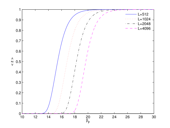
Figure 4: Order parameter $\langle{{{z}}}\rangle$ in $d=2$ along $\beta_{F}$ for $L=512$, 1024, 2048 and 4096.

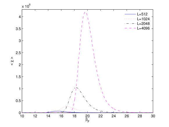
Figure 5: Susceptibility $\chi_{{z}}$ in $d=2$ along $\beta_{F}$ for $L=512$, 1024, 2048 and 4096.

We can clearly distinguish a low $\beta_{F}$, “strong” coupling regime, where $\langle{{z}}\rangle=0$ and the topology is ill defined, from a high $\beta_{F}$, “weak” coupling one, where $\langle{{z}}\rangle=1$, the correct value it should have if the vacuum satisfies Eq. (4). For higher $L$ the transition “front” simply moves to the right, i.e. higher $\beta_{F}$; see Fig. 7, where the curves along which the susceptibility $\chi_{{z}}$ peaks are plotted for $L=64$, 256, 1024 and 4096.

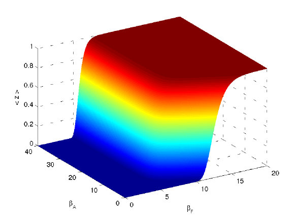
Figure 6: Order parameter $\langle{{{z}}}\rangle$ in $d=2$ for fixed $L=128$.

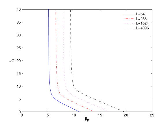
Figure 7: Peak curves of the susceptibility $\chi_{{z}}$ in the $\beta_{F}-\beta_{A}$ plane for $L=64$, 256, 1024 and 4096.

As usual in a FSS analysis, we can determine the properties of the transition by defining the pseudo-critical couplings $(\beta^{c}_{F}(L),\beta^{c}_{A}(L))$ at finite $L$ as those for which the correlation length $\xi\simeq L$ Fisher and Barber (1972). These can be identified through the peaks of the susceptibility $\chi_{{z}}$ (see Fig. 7); since $p(\beta_{F},\beta_{A})$ has no stationary points, from Eq. (17) one simply needs to solve:

$$p(\beta^{c}_{F},\beta^{c}_{A})=\frac{\log{2}}{4\,L^{2}}\,.$$ (18)

Substituting the above value into Eq. (17) we get for the scaling of the center flux and its susceptibility with $L$:

$${{z}}(\beta^{c}_{F},\beta^{c}_{A}) = \frac{1}{2}$$

$$\chi_{{z}}(\beta^{c}_{F},\beta^{c}_{A}) = \frac{L^{2}}{4}\,.$$ (19)

As for the scaling of the pseudo-critical points with $L$, from Eqs. (15) we have that along lines parallel to the $\beta_{A}$ axis $\langle{{z}}\rangle=0$. Otherwise, we can fix a line $\beta_{A}=f(\beta_{F})$ and solve:

$$p(\beta_{F},f(\beta_{F}))=\frac{\log{2}}{4\,L^{2}}$$ (20)

for $\beta_{F}$. In particular, from Eq. (16) and using the asymptotic expansion Abramowitz and Stegun (1964):

$$p(\beta_{F},\beta_{A}\equiv 0)\sim\sqrt{\frac{2\beta_{F}}{\pi}}\mathrm{e}^{-\beta_{F}}\,\left[1+{\cal{O}}(\frac{1}{\beta_{F}})\right]$$ (21)

we get for the two limiting cases $\beta_{A}\to 0\,,\infty$:

$$\beta^{c}_{F}(L)|_{\beta_{A}=0} \sim \log{L^{2}}+\frac{1}{2}\log{\log{L^{2}}}+{\cal{O}}(1)$$ (22)

$$\beta^{c}_{F}(L)|_{\beta_{A}=\infty} \sim \frac{1}{2}\log{L^{2}}+{\cal{O}}(1)\,:$$ (23)

shifting Eqs. (17) by Eqs. (22, 23) $\langle{{z}}\rangle$ and $\langle\chi_{{z}}\rangle$ will fall on top of each other.

Inverting Eqs. (22, 23), one can extract the critical behaviour of the correlation length $\xi\sim L$ for $\beta_{A}\to 0\,,\infty$, where the pre-factors come from the ${\cal{O}}(1)$ terms:

$$\xi|_{\beta_{A}=0}\; \sim \sqrt[4]{\frac{\pi\log^{2}{2}}{2\beta_{F}}}\;\cdot\,\mathrm{e}^{\frac{1}{2}\beta_{F}}$$ (24)

$$\xi|_{\beta_{A}=\infty} \sim \sqrt{\frac{\log{2}}{4}}\;\cdot\,\mathrm{e}^{\beta_{F}}\,.$$ (25)

Similar expressions will hold for any direction $\beta_{A}=f(\beta_{F})$ along which the continuum limit $\beta_{F}\to\infty$ is taken. At $T>0$ one can simply substitute $L^{2}\to L_{s}\cdot L_{t}$ in Eqs. (18, 19, 22, 23). The scaling behaviour remains thus, up to a factor, unchanged when taking the thermodynamic limit $L_{s}\to\infty$: the critical behaviour will persist for any fixed $L_{t}$, i.e. at any temperature.

Compare now the above scaling with the critical behaviour of the Kosterlitz-Thouless universality class Kenna and Irving (1997); Kosterlitz and Thouless (1973); Kosterlitz (1974) as a function of the reduced coupling $\beta_{\mathrm{red}}$:

$$\xi_{KT}\sim \,K\,\mathrm{e}^{A\,\beta_{\mathrm{red}}^{\nu}}$$ (26)

$$\beta_{\mathrm{red}}^{-1}= \left|\beta^{-1}-\beta^{-1}_{c}\right|\propto\left|T-T_{c}\right|\,.$$ (27)

Albeit with a different critical exponent, $\nu=1$ and $\nu=1/2$ respectively, both cases show essential scaling, i.e. the correlation length diverges exponentially as one approaches the critical coupling, which in our case is $\beta^{c}_{F}=\infty$. Mimicking now a well-known argument Kosterlitz and Thouless (1973); Kosterlitz (1974), we can give a simple explanation for the behaviour found in Eqs. (24, 25). At weak coupling the free energy cost to change the sign of a plaquette is $f\sim 2\beta_{F}$; the density of negative plaquettes will thus be controlled by a Boltzmann factor $\rho\sim\exp{(-f)}$. On the other hand the possible positions for this sign flip will scale like $L^{2}$ and the balance between free energy and entropy gives $L\sim\rho^{-1/2}=\exp{(\beta_{f})}\simeq\xi$. Up to the power correction for $\beta_{A}=0$ case, Eq. (24), this simple argument works quite well, contrary to the $XY$-model, where it cannot explain renormalization effects leading to the non trivial critical exponent $\nu=1/2$. Moreover, since the minimal distance among vortices can be reliably estimated with that along a plane intersecting them, such picture should (roughly) hold in higher dimensions as well.

We could in principle explore the similarities with the Kosterlitz-Thouless transitions further. Although, as far as we know, for the $XY$-model no local order parameter is available, one can couple the theory to an external magnetic field $h$ and study the analytical continuation of the partition function $Z(\beta,h)$ to the complex plane. (Hyper-) scaling relations will then hold among the critical exponents of $\xi$, of the magnetic susceptibility $\chi_{h}\sim\xi^{2-\eta}\log^{-2r}{\xi}$, of the specific heat $C_{s}$ and of the edge of the Lee-Yang zeroes Kenna and Irving (1997). We will avoid such a throughout analysis in our case, for which a dedicated paper would be needed. Let us however just briefly comment on two points. First, from Eq. (13) we can explicitly calculate the reduced partition function and the specific heat in our usual limiting cases:

$$Z\underset{\beta_{A}\to 0}{\propto} \;\frac{1}{\beta_{F}}\,I_{1}(\beta_{F})$$ (28)

$$Z\underset{\beta_{A}\to\infty}{\propto} \,\frac{\mathrm{e}^{\beta_{A}}}{\sqrt{\beta_{A}^{3}}}\,\cosh{\beta_{F}}$$ (29)

$$C_{s}\underset{\beta_{A}\to 0}{=} \;\frac{3}{2\,\beta^{2}_{F}}$$ (30)

$$C_{s}\underset{\beta_{A}\to\infty}{=} \;1-\tanh^{2}{\beta_{F}}\,.$$ (31)

Inserting Eqs. (22, 23) into Eqs. (30, 31) and assuming that no other contribution besides the singular one exist Kenna and Irving (1997), we see that the critical behaviour for $C_{s}$ should change (continuously?) from $\log^{-2}L$ to $L^{-2}$. Second, in our case we have direct access to a non local, topological order parameter, for which we can determine a critical exponent, ${{z}}\sim M\,L^{-\beta}$; from Eq. (19) we have $\beta=0$. If we would like to study the extended partition function $Z(\beta_{F},\beta_{A},h)$ we could simply add a term $S_{h}=h\,{{z}}$ to the action. Although a direct calculation would go beyond the scope of this paper, it is obvious that for fixed $L$ a sufficient condition to align the center flux ${{z}}$ is realized if $\beta_{F}\to\infty$: the fundamental coupling plays the role of a ”mock” $\mathbb{Z}_{2}$ magnetic field. Indeed, from Eqs. (28, 29) the zeros of $Z$ in the complex $\beta_{F}$ plane all lie on the imaginary axis, in agreement with the Lee-Yang theorem Lee and Yang (1952).

Let us finally turn to the continuum limit. From the above discussion it is clear that taking the thermodynamic limit $L\to\infty$ before the weak coupling limit $\beta_{F}\to\infty$, as one should, i.e. taking the Euclidean volume $V=(a\,L)^{2}\to\infty$ (or, at finite temperature, $V_{s}=(a\,L_{s})\to\infty$), the theory remains stuck in the disordered phase $\langle{{z}}\rangle=0$: no vortex topological sector can be defined and the super-selection rule of Eq. (2) is not realized.

On the other hand, assuming that the scaling of the string tension $\sigma$ with the lattice spacing $a$, known analytically for $\beta_{A}=0$:

$$\beta_{F} = \frac{4}{a^{2}\,g^{2}}$$

$$\sigma = \frac{3}{8}\,g^{2}\,,$$ (32)

will hold up to a different prefactor along any line $f(\beta_{F})\propto\beta_{F}$, we get:

$$V=(a\,L)^{2}=\frac{3}{2}\frac{L^{2}}{\sigma\,\beta_{F}}\,.$$ (33)

Keeping now the volume $V$ fixed as the continuum limit is approached, the values of the coupling at which one needs to simulate for fixed $L$ will scale as $\beta_{F}\sim{L^{2}}$, i.e. much higher than the pseudo-critical coupling $\beta^{c}_{F}\sim\log{L}$. The theory will thus be in a pseudo-ordered phase with $\langle{{z}}\rangle=1$: on a finite Euclidean $d=2$ torus the Wilson action can admit well defined $\mathbb{Z}_{2}$ topological sectors.

III.2 $d=3$

Increasing the dimensions to $d=3$ we expect interactions to arise among parallel planes, since vortices are now extended, one-dimensional objects. The simple picture we have found in $d=2$ won’t probably work anymore and less trivial critical exponents might arise. Still, fluxes are inherently two-dimensional objects and most of the dynamics should thus take place on planes: many features of the $d=2$ case should therefore survive. To check this, we have performed sets of Monte-Carlo simulations along different lines in the $\beta_{F}-\beta_{A}$ plane. Results are reported for $\beta_{A}=0$, $\beta_{F}=0.5$, $0.75$ and lattice sizes between $L=24$ and $L=80$; other parameters have been checked and give a consistent picture.

In the $\beta_{A}=0$ case approximately 20 to 50 simulations at coupling steps $\delta\beta_{F}$, each with $10^{6}$ independent configurations, were performed for each volume $L^{3}$. The data have been re-weighted Ferrenberg and Swendsen (1988, 1989) to determine the peak values $\beta^{c}_{F}(L)$ and $\chi_{{z}}(\beta^{c}_{F}(L))$; this was viable only up to $L\sim 64$. Indeed, as we shall see below, the $d=3$ case shows a similar scaling behaviour as Eq. (22), i.e. a logarithmic scaling of $\beta_{F}^{c}(L)$ to a critical coupling $\beta_{F}^{c}=\infty$. This has a practical drawback: the absolute width of the transition, i.e. the overall interval $\Delta\beta_{F}$ one needs to simulate, varies very slowly, while the step-width $\delta\beta_{F}$ one must scan in order to keep the density of states computationally feasible decreases dramatically with $L$: the computational cost becomes eventually unmanageable.

Results for all volumes considered are resumed in Tab. 1, where the steps $\delta\beta_{F}$ are also listed, along with the value of the center flux and, for sake of completeness, of the specific heat at the pseudo-critical point. To cross-check scaling results, similar simulation steps and statistics have also been used for the other volumes not included in the re-weighting.

	$L=24$	$L=32$	$L=40$	$L=48$	$L=64$
$\beta^{c}_{F}(L)$	$5.61(1)$	$5.930(5)$	$6.174(2)$	$6.383(5)$	$6.700(5)$
$\chi_{{z}}(\beta^{c}_{F}(L))$	$152.90(4)$	$282.83(8)$	$454.24(12)$	$666.6(2)$	$1217.4(3)$
${{z}}(\beta^{c}_{F}(L))$	$0.392(3)$	$0.3610(15)$	$0.3364(13)$	$0.3213(16)$	$0.2908(16)$
$C_{s}(\beta^{c}_{F}(L))$	$0.1078(3)$	$0.0957(1)$	$0.0877(2)$	$0.0817(3)$	$0.0739(4)$
$\delta\beta_{F}$	$0.025$	$0.0125$	$0.00625$	$0.003125$	$0.0015625$

Table 1: Position and height of the susceptibility peaks along $\beta_{F}$ in $d=3$. The third and fourth line give the values of the order parameter and of the specific heat at the pseudo-critical point $\beta^{c}_{F}(L)$; the last line gives the coupling steps for the simulations used in the re-weighting.

The data can be well fitted with the Ansatz:

$$\chi_{{z}}(\beta^{c}_{F}(L)) \sim A\,L^{2-\eta}\log^{-2r}{L}\left(1+{\cal{O}}(L^{-1})\right)$$ (34)

$${{z}}(\beta^{c}_{F}(L)) \sim M\,L^{-\beta}\left(1+{\cal{O}}({L}^{-1})\right)$$ (35)

$$\beta^{c}_{F}(L) \sim C\,\log{L^{2}}+D\,\log\log{L^{2}}+{\cal{O}}(1)\,,$$ (36)

For $\chi_{{z}}$ we get $A=0.21(1)$, $r=-0.134(10)$, $\eta=0.0001(100)$ and $\chi^{2}$/d.o.f.$=5.7$; constraining $\eta=0$ gives again $A=0.21(1)$, $r=-0.134(10)$ with $\chi^{2}$/d.o.f.$=2.8$. For $\beta_{F}^{c}$ we get $C=0.61(3)$ and $D=-0.42(5)$ with $\chi^{2}$/d.o.f.$=0.7$; on the other hand, constraining $D=0$ we get $C=0.56(3)$, $\chi^{2}$/d.o.f.$=0.6$. Finally, for the order parameter, we get $M=1.26(5)$ and $\beta=0.35(1)$ with $\chi^{2}$/d.o.f.$=1.4$. Overall, the biggest source of systematic error is given by the parameterization of the sub-leading corrections: leaving them out or parameterizing them differently leads to changes of up to $10\%$ for some of the critical exponents, not included in our error estimates; obviously, more data at higher volumes are needed to pin the numbers down. The data for the susceptibility $\chi_{{z}}$, rescaled by Eqs. (34, 36), are plotted in Fig. 8, showing very good agreement also for the volumes which have not been included in the re-weighting analysis.

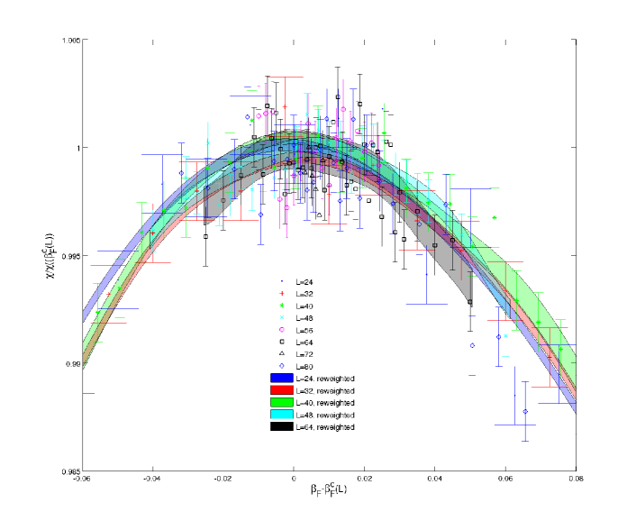
Figure 8: Data for the susceptibility of the order parameter in $d=3$, including the re-weighted curves, rescaled with the FSS Ansatz in Eqs. (34, 36).

In Fig. 9 we show the scaling of the order parameter ${{z}}$ according to Eqs. (35, 36); the agreement for $L\gtrsim 40$ is again very good.

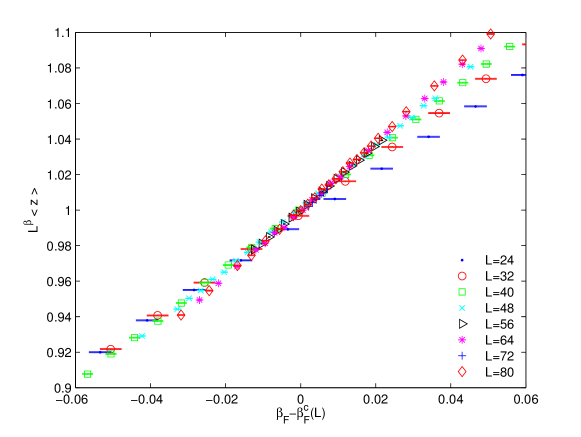
Figure 9: FSS for the order parameter ${{z}}$ as a function of the rescaled coupling as in Eq. (35).

As for the specific heat, a fit of the data in Tab. 1 with a logarithmic Ansatz $C_{s}\sim\log^{-\alpha}{L}$ gives $\alpha=1.4(1)$ with a $\chi^{2}$/d.o.f.$=0.5$. The signal-to-noise ratio for the MC is however not so good in this case, reflecting itself in the quality of the re-weighted data: more statistics would be definitely needed; anyway, checking any (hyper-) scaling relation is beyond our goals.

The above result is quite surprising. Indeed, in contrast to $d=2$, one could have expected the $\mathbb{Z}_{2}$ monopole to control the open center vortices, since the density of the latter is proportional to that of the former. However, although monopoles per unit volume steadily decrease beyond the cross-over, open vortices “connecting” them still cause a critical behaviour cumulating to $g^{2}\to 0$. A possible explanation could be that their length increases more than linearly with the lattice size; multiple bendings in orthogonal directions would be enough to randomize the fluxes. A direct investigation of any geometrical properties of open vortices is however beyond the scope of this paper, since Eq. (9) is non local and gauge invariant and does not allow to isolate the topological defects on the planes.

Going now to the $\beta_{A}\neq 0$ case, since the $\mathbb{Z}_{2}$ monopoles undergo a cross-over also in the low $\beta_{F}$ region of the phase diagram of Fig. 2, one would expect the center flux to behave as in the $\beta_{F}$ case: one should find along $\beta_{A}$ a similar scaling as in Eqs. (34, 36). Also, the transition lines should not be effected by the bulk transition associated with the unphysical $\mathbb{Z}_{2}$ gauge degrees of freedom. However, such strong transition unavoidably makes any simulation near it quite noisy; on top of that the biased Metropolis algorithm, with e.g. 3 micro-canonical steps, gets inefficient as $\beta_{F}$ gets small and $\beta_{A}$ large, reaching for ${{z}}$ and $\chi_{{z}}$, around the peaks of the latter, integrated autocorrelation times of the order $10^{4}-10^{5}$ for $24\leq L\leq 40$. Passable data were therefore only accessible for three volumes, while gathering enough statistics to re-weight the susceptibility was out of the question. We have thus limited ourself to a consistency check near the bulk transition with a scaling Ansatz similar to Eqs. (34-36):

$$\chi_{{z}}(\beta^{c}_{A}(L)) \sim A\,L^{2}\log^{-2r}{L}+{\cal{O}}(L)$$ (37)

$${{z}}(\beta^{c}_{A}(L)) \sim M\,L^{-\beta}\left(1+{\cal{O}}({L}^{-1})\right)$$ (38)

$$\beta^{c}_{A}(L) \sim C\,\log{L^{2}}+{\cal{O}}(1)\,;$$ (39)

no fit has been attempted. The scaling of the pseudo critical point and of the order parameter are consistent with the $d=2$, $\beta_{A}=\infty$ case, $C=1/2$ and $\beta=0$, as can be seen from Fig. 10.

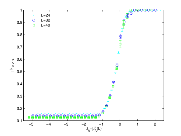
Figure 10: FSS for the order parameter ${{z}}$ along the $\beta_{F}=0.5$ line with the Ansatz in Eqs. (37, 38).

On the other hand, the peaks of $\chi_{{z}}$ are quite noisy and even a consistency check for the logarithmic exponent is hopeless. In Fig. 11, 12 we show the results for the simulations along $\beta_{F}=0.5$ and $\beta_{F}=0.75$, lying respectively left and right of the bulk transition, rescaled by Eq. (37, 39) with a “guessed” value for $r=-1/2$; of course, further work would be needed to determine the critical exponents reliably.

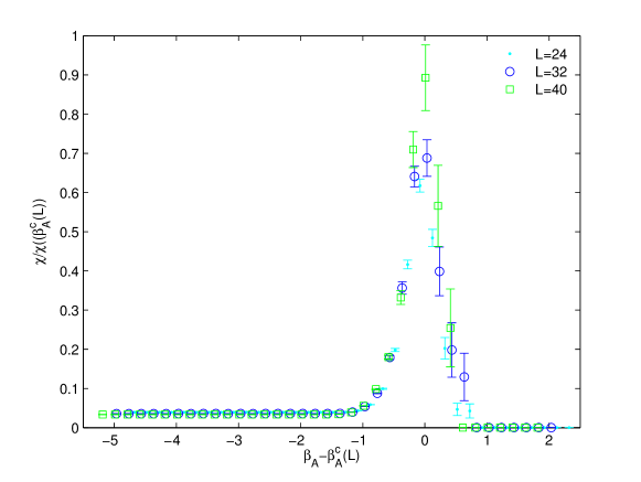
Figure 11: FSS for the susceptibility $\chi_{{z}}$ along the $\beta_{F}=0.5$ line with the Ansatz Eqs. (37, 39).

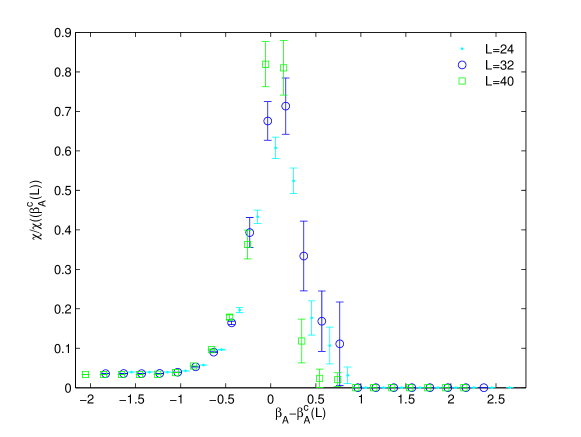
Figure 12: FSS for the susceptibility $\chi_{{z}}$ along the $\beta_{F}=0.75$ line with the Ansatz Eqs. (37, 39).

We have also checked via Monte-Carlo simulations that all of the above results generalize to $T>0$ by simply substituting $L^{2}\to L_{s}\cdot L_{t}$ in all the scaling relations for temporal fluxes, while the behaviour of all spacial fluxes remains unchanged. Again, as in the $d=2$ case, this implies that, along any line in the $\beta_{F}-\beta_{A}$ plane, when taking the thermodynamic limit before the weak coupling limit, i.e. sending the volume to infinity, the $d=3$ theory remains stuck in the disordered phase $\langle{{z}}\rangle=0$; again, Eq. (2) is not realized.

What about the fixed volume limit? Taking as a blueprint for the continuum limit along any direction the scaling of the string tension along $\beta_{F}$ Teper (1999):

$$\beta_{F} = \frac{4}{a\,g^{2}}$$

$$a\,\sqrt{\sigma} = \frac{c_{0}}{\beta_{F}}+\frac{c_{1}}{\beta^{2}_{F}}+{\cal{O}}(\frac{1}{\beta^{3}_{F}})\,.$$ (40)

we get immediately:

$$V=(a\,L)^{3}\propto\frac{L^{3}}{\beta_{F}^{3}\sqrt{\sigma^{3}}}\,.$$ (41)

Keeping again $V$ fixed as the continuum limit is approached, the values of the coupling corresponding to a given $L$ will now scale as $\beta_{F}\sim{L}$; again, as in $d=2$, they will always be much higher than the pseudo-critical coupling $\beta^{C}_{F}\sim\log{L}$ and the Wilson action could admit well defined $\mathbb{Z}_{2}$ topological sectors on a finite $d=3$ torus.

III.3 $d=4$

The positions of the peaks of $\chi_{{z}}$, as obtained in the simulations along the $\beta_{A}=0$, $\beta_{F}=1.0$, $\beta_{F}=1.2$ and $\beta_{F}=1.3$ lines, all within phase I of Fig. 3, are shown in Tabs. 2, 3.

	$L=12$	$L=16$	$L=20$	$L=24$
$\beta^{c}_{F}(L)$	$3.15(5)$	$3.40(5)$	$3.60(5)$	$3.75(5)$
$\chi_{{z}}(\beta^{c}_{F}(L))$	$24(1)$	$42(1)$	$66(1)$	$95(1)$

Table 2: Position and height of the susceptibility peaks along $\beta_{F}$ in $d=4$.

	$L=16$	$L=20$	$L=24$
$\beta_{F}=1.0$	$1.845(25)$	$1.923(25)$	$1.987(25)$
$\beta_{F}=1.2$	$1.695(25)$	$1.773(25)$	$1.837(25)$
$\beta_{F}=1.3$	$1.62(1)$	$1.70(10)$	$1.76(1)$

Table 3: Position of the susceptibility peaks along $\beta_{A}$ in $d=4$ for $\beta_{F}=1.0$, 1.2 and 1.3; the heights are all compatible with the results in Tab. 2

We have again limited ourselves to a consistency check with a scaling Ansatz of the form:

$$\chi_{{z}}(\beta^{c}_{F}(L)) \sim A\,L^{2}+{\cal{O}}(L)$$ (42)

$${{z}}(\beta^{c}_{F}(L)) \sim M\,L^{-\beta}\left(1+{\cal{O}}({L}^{-1})\right)$$ (43)

$$\beta^{c}_{F}(L) \sim C\,\log{L^{2}}+{\cal{O}}(1)\;.$$ (44)

Results are shown in Figs. 13, 14 for the order parameter and its susceptibility along the $\beta_{F}$ axis; up to the values of $C$ the behaviour along the lines parallel to the $\beta_{A}$ axis is basically the same, see e.g. Fig. 15. From the data in Tab. 2 we can estimate $C=0.46(3)$, compatible with $1/2$, while for those in Tab. 3 we get $C=0.18(3)$; in all cases $\beta$ is compatible with 0.

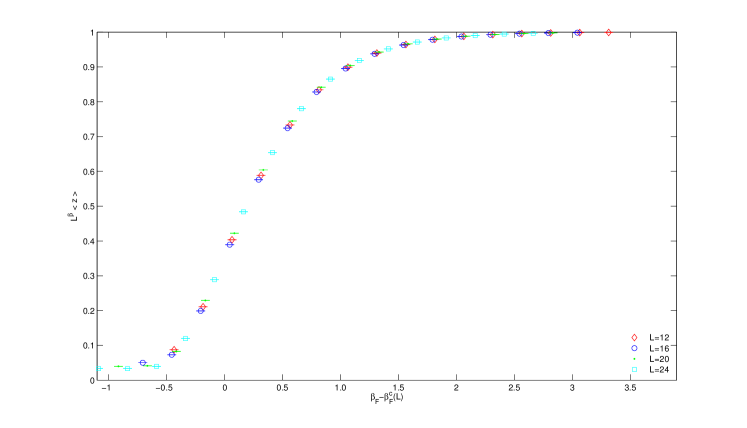
Figure 13: FSS as in Eqs. (43, 44) for ${{z}}$ in $d=4$ along the $\beta_{F}$ axis.

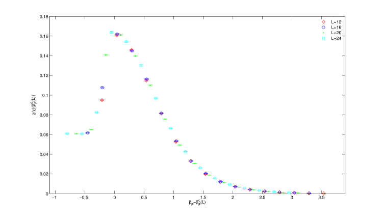
Figure 14: FSS as in Eqs. (42, 44) for $\chi_{{z}}$ in $d=4$ along the $\beta_{F}$ axis.

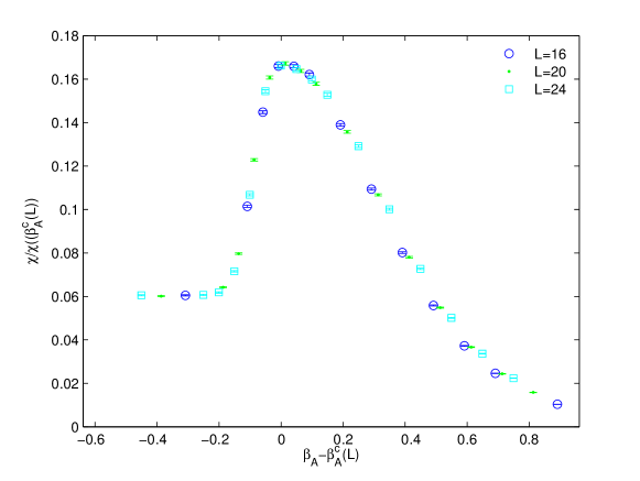
Figure 15: FSS as in Eqs. (42, 44) for $\chi_{{z}}$ in $d=4$ along the $\beta_{F}=1.3$ axis.

Direct simulations at $T>0$ give again the same scaling with $L^{2}\to L_{s}\cdot L_{t}$ for the temporal fluxes, while spacial fluxes remain unchanged. As in the $d=2$ and $d=3$ cases, in the thermodynamic limit the theory remains therefore stuck in the disordered phase. Moreover, starting from the 2-loop beta-function, the running of the physical scale with $\alpha_{\mathrm{lat}}=g^{2}/(4\,\pi)$ is given by:

$$\log{\left(a^{2}\,\sigma\right)}=-\frac{4\,\pi}{\beta_{0}}\,\alpha_{\mathrm{lat}}^{-1}+\frac{2\,\beta_{1}}{\beta_{0}^{2}}\,\log{\left(\frac{4\,\pi}{\beta_{0}}\,\alpha_{\mathrm{lat}}^{-1}\right)}+c+{\cal{O}}(\alpha_{\mathrm{lat}})\,,$$ (45)

where $c=\log{\frac{\sigma}{\Lambda^{2}_{\mathrm{lat}}}}$ and $\beta_{0}=\frac{22}{3}$, $\beta_{1}=\frac{68}{3}$, i.e. from Eq. (7):

$$V=(a\,L)^{4}\propto{L^{4}}\,\left(\frac{4\,\pi^{2}}{\beta_{0}}\,\beta_{F}\right)^{\frac{4\,\beta_{1}}{\beta_{0}^{2}}}\,\mathrm{e}^{-\frac{8\,\pi^{2}}{\beta_{0}}\,\beta_{F}}\,.$$ (46)

When trying to keep the volume $V$ fixed as $\beta_{F}\to 0$, up to $\log\log$ corrections the coupling should scale as:

$$\beta_{F}\sim\frac{\beta_{0}}{4\,\pi^{2}}\,\log{L^{2}}\,;$$ (47)

the coefficient $C$ in Eq. (44) is however larger than that coming from the beta-function and the simulation parameters will lie in the disordered phase: topological sectors will always be ill-defined also on a finite torus $T^{4}$. The same holds along the lines parallel to the $\beta_{A}$ axis (see Tab. 3); in this case, from Eq. (7), the coefficient in Eq. (47) coming from the beta-function Eq. (45) is ${3\,\beta_{0}}/({32\,\pi^{2}})$, again smaller than the corresponding value of $C$.

As discussed in Sec. II.2, we have excluded phase II (see Fig. 3) from the simulations. As mentioned above, vortex topology is however well understood in this case: the results of Refs. Barresi et al. (2004a, b); Barresi and Burgio (2007); Burgio et al. (2006a, 2007) show that, in contrast to phase I in $d=4$ and to the $d=2$ and 3 cases, the theory possesses well defined $\mathbb{Z}_{2}$ topological sectors in the continuum limit.

IV Conclusions

We have studied a topological order parameter, the center flux $z$ defined in Eqs. (10, 11), for the $SU(2)$ mixed action in $2\leq d\leq 4$. Its ordered phase, $\langle z\rangle=1$, corresponds to well defined $\pi_{1}(SO(3))=\mathbb{Z}_{2}$ topological sectors, i.e. to a vacuum satisfying the super-selection rule of Eqs. (2, 4), while for $\langle z\rangle=0$ the vacuum state is disordered and no center topology can be defined. This reminds of a quantum phase transition; however, one does not switch between vacua by tuning a physical parameter. Rather, the choice of dimensions and the symmetry of the discretized action control in which phase the theory will be in the continuum limit.

More specifically, discretized actions transforming in the fundamental representation possess a disordered vacuum, with $z$ showing an essential scaling to the critical coupling $\beta_{c}=\infty$. The critical exponent for the correlation length $\xi$ is $\nu=1$, i.e. $\beta_{c}(\xi)\propto\log{\xi}$; explicit $\log\log{\xi}$ corrections to scaling can be shown to exist for some choice of parameters. The susceptibility of the center flux scales as $\chi_{{z}}(\xi)\propto\xi^{2}$ in $d=2$ and $d=4$, while the order parameter itself scales trivially in these cases. On the other hand in $d=3$, at least along the $\beta_{F}$ axis, the center flux has a non trivial critical exponent, ${{z}}(\xi)\propto\xi^{-\beta}$, with $\beta=0.35(1)$, while a logarithmic correction can be explicitly determined for the scaling of its susceptibility, $\chi_{{z}}(\xi)\sim\xi^{2}\,\log^{-2r}{\xi}$, with $r=-0.134(10)$; similar corrections might also be present along other lines in the $\beta_{F}-\beta_{A}$ diagram, but more statistics would be needed to reach a conclusive result. A tentative critical exponent for the specific heat, $C_{s}(\xi)\sim\log^{-\alpha}{\xi}$, gives $\alpha=1.4(1)$, but with still high systematic errors. We have made no attempt to investigate any (hyper-) scaling relations among such exponents; this would probably require a full analysis of the Lee-Yang zeros Kenna and Irving (1997). Such behaviour persists in all dimensions at $T>0$.

Vice versa, the topological classification of Eq. (1) and thus the super-selection rule of Eqs. (2, 4) can be realized by the vacuum state of lattice actions transforming in the adjoint representation; phase II in $d=4$ (see Fig. 3) is such an example Burgio et al. (2006a, 2007); Barresi and Burgio (2007). Large scale simulations with the adjoint action are hampered by strong finite-volume effects Halliday and Schwimmer (1981b, a); de Forcrand and Jahn (2003). Therefore, although the techniques used in Refs Burgio et al. (2006a, 2007); Barresi and Burgio (2007) to tame them could also work in $d=3$, a more viable alternative, applicable also in $d=2$, would be to resort to positive plaquette models Mack and Pietarinen (1982); Bornyakov et al. (1991); Fingberg et al. (1995), where topological sectors are always well defined since the operator given in Eq. (9) takes “by construction” the values dictated by the assigned boundary conditions. Indeed, a one-to-one mapping between configurations in such lattice discretization and those of the adjoint Wilson action with well defined vortex sectors was conjectured in Ref. de Forcrand and Jahn (2003) and explicitly constructed in Ref. Barresi and Burgio (2007). Finally, an ordered vacuum could also be realized for a finite torus in $d=2,\,3$; here one could exploit the power-law scaling of the physical mass with the coupling to define topological sectors when $L\to\infty$ and $a\to 0$ with the volume $V=(a\,L)^{d}$ kept fixed.

The above findings do not contradict universality, since non perturbatively the equivalence between fundamental and adjoint actions can only hold as long as no lattice artifacts are present Mack and Petkova (1979, 1982); Halliday and Schwimmer (1981b, a); Coleman (1982); de Forcrand and Jahn (2003); Barresi and Burgio (2007), while as we have seen for some discretizations the density of $\mathbb{Z}_{2}$ monopoles can not vanish at any finite coupling Mack and Petkova (1982). Does however such result have any physical consequences? The vacua of the two different phases can be essentially characterized by the type of $\mathbb{Z}_{2}$ vortices they can carry:

i) The ordered phase allows topological center vortices “à la ’t Hooft” ’t Hooft (1978, 1979): a confinement mechanism based on the super-selection rule of Eqs. (2, 4) can be realized; at finite temperature the change in the vortex free energy as measured via Eq. (3) is thus a valid test to establish how the symmetry is broken in the transition to the deconfined phase Burgio et al. (2006a, 2007); Barresi and Burgio (2007). No fundamental fields are allowed in this case ’t Hooft (1978, 1979); Cohen (2014); however, adjoint fermions can be easily incorporated in such scenario. It might therefore be interesting to investigate the vacuum properties of the $SU(2)$ gauge theory coupled to adjoint fermions, a popular candidate for infrared conformality Lucini et al. (2013). Numerical tests with the adjoint Wilson action or positive plaquette model should be viable.

ii) The disordered phase is dominated by (one huge, percolating?) open vortices, reminding of the Nielsen-Olesen “spaghetti vacuum” Nielsen and Olesen (1973). Such open vortices are not topological according to Eq. (1): Eqs. (2, 4) cannot be applied. One might conjecture some relationship with P-vortices Del Debbio et al. (1997); Langfeld et al. (1998); Greensite (2011), although it is still unclear how to test such hypothesis, since the center flux $z$ is gauge invariant and constructed out of pure $SO(3)$ variables while P-vortices are gauge dependent and built out of the $\mathbb{Z}_{2}$ gauge degrees of freedom. Moreover, such open vortices persist at any temperature, not disappearing above $T_{C}$. This disordered vacuum is detached from the boundary conditions chosen and is therefore compatible with the presence of fundamental matter fields. Of course, Eq. (3) is ill defined in this case; whether any vortex related order parameter for the confinement-deconfinement phase transition could be defined remains an open question.

Aknowledgements

We are indebted to F. Bursa for precious correspondence on the $d=2$ Yang-Mills theory. We want to thank B. Lucini, P. de Forcrand and D. Campagnari for critical reading of the manuscript; we also wish to thank R. Kenna for interesting discussions on Lee-Yang and Fisher zeroes. A special thanks goes to E. Rinaldi for correspondence on the implementation of the biased Metropolis algorithm. This work was supported by the Bundesministerium für Bildung und Forschung under the contract BMBF-05P12VTFTF.

References

- Jaffe and Witten (2000) A. M. Jaffe and E. Witten, Clay Mathematics Institute Millenium Prize problem (2000), http://www.claymath.org/millennium/Yang-Mills_Theory/yangmills.pdf.
- Greensite (2011) J. Greensite, An introduction to the confinement problem, Vol. 821 (Springer Verlag, Berlin, Heidelberg, 2011) pp. 1–211.
- Wu and Yang (1969) T. Wu and C.-N. Yang, in Properties Of Matter Under Unusual Conditions, edited by H. Mark and S. Fernbach (Interscience, New York, 1969).
- Nielsen and Olesen (1973) H. B. Nielsen and P. Olesen, Nucl.Phys. B61, 45 (1973).
- ’t Hooft (1974) G. ’t Hooft, Nucl. Phys. B79, 276 (1974).
- Mandelstam (1975) S. Mandelstam, Phys.Lett. B53, 476 (1975).
- Polyakov (1977) A. M. Polyakov, Nucl. Phys. B120, 429 (1977).
- Goddard et al. (1977) P. Goddard, J. Nuyts, and D. I. Olive, Nucl.Phys. B125, 1 (1977).
- Mandelstam (1979) S. Mandelstam, Phys.Rev. D19, 2391 (1979).
- Weinberg (1980) E. J. Weinberg, Nucl.Phys. B167, 500 (1980).
- Seiberg and Witten (1994) N. Seiberg and E. Witten, Nucl.Phys. B426, 19 (1994), arXiv:hep-th/9407087 [hep-th] .
- ’t Hooft (1978) G. ’t Hooft, Nucl.Phys. B138, 1 (1978).
- ’t Hooft (1979) G. ’t Hooft, Nucl.Phys. B153, 141 (1979).
- Mack and Pietarinen (1982) G. Mack and E. Pietarinen, Nucl.Phys. B205, 141 (1982).
- Del Debbio et al. (1997) L. Del Debbio, M. Faber, J. Greensite, and S. Olejnik, Phys.Rev. D55, 2298 (1997), arXiv:hep-lat/9610005 [hep-lat] .
- Langfeld et al. (1998) K. Langfeld, H. Reinhardt, and O. Tennert, Phys.Lett. B419, 317 (1998), arXiv:hep-lat/9710068 [hep-lat] .
- Kovacs and Tomboulis (2000) T. G. Kovacs and E. Tomboulis, Phys.Rev.Lett. 85, 704 (2000), arXiv:hep-lat/0002004 [hep-lat] .
- Hart et al. (2000) A. Hart, B. Lucini, Z. Schram, and M. Teper, JHEP 0006, 040 (2000), arXiv:hep-lat/0005010 [hep-lat] .
- de Forcrand et al. (2001) P. de Forcrand, M. D’Elia, and M. Pepe, Phys.Rev.Lett. 86, 1438 (2001), arXiv:hep-lat/0007034 [hep-lat] .
- de Forcrand and von Smekal (2002) P. de Forcrand and L. von Smekal, Phys.Rev. D66, 011504 (2002), arXiv:hep-lat/0107018 [hep-lat] .
- Burgio et al. (2006a) G. Burgio, M. Fuhrmann, W. Kerler, and M. Muller-Preussker, Phys.Rev. D74, 071502 (2006a), arXiv:hep-th/0608075 [hep-th] .
- Burgio et al. (2007) G. Burgio, M. Fuhrmann, W. Kerler, and M. Muller-Preussker, Phys.Rev. D75, 014504 (2007), arXiv:hep-lat/0610097 [hep-lat] .
- von Smekal (2012) L. von Smekal, Nucl.Phys.Proc.Suppl. 228, 179 (2012), arXiv:1205.4205 [hep-ph] .
- Gonzalez-Arroyo (1997) A. Gonzalez-Arroyo, (1997), arXiv:hep-th/9807108 [hep-th] .
- Burgio et al. (2000) G. Burgio, R. De Pietri, H. A. Morales-Tecotl, L. F. Urrutia, and J. D. Vergara, Nucl. Phys. B566, 547 (2000), arXiv:hep-lat/9906036 .
- Reinhardt (2003) H. Reinhardt, Phys.Lett. B557, 317 (2003), arXiv:hep-th/0212264 [hep-th] .
- de Forcrand and Jahn (2003) P. de Forcrand and O. Jahn, Nucl.Phys. B651, 125 (2003), arXiv:hep-lat/0211004 [hep-lat] .
- Halliday and Schwimmer (1981a) I. Halliday and A. Schwimmer, Phys.Lett. B102, 337 (1981a).
- Barresi and Burgio (2007) A. Barresi and G. Burgio, Eur.Phys.J. C49, 973 (2007), arXiv:hep-lat/0608008 [hep-lat] .
- Svetitsky and Yaffe (1982) B. Svetitsky and L. G. Yaffe, Nucl.Phys. B210, 423 (1982).
- Cohen (2014) T. D. Cohen, Phys.Rev. D90, 047703 (2014), arXiv:1407.4128 [hep-th] .
- Gonzalez-Arroyo and Okawa (1983) A. Gonzalez-Arroyo and M. Okawa, Phys.Rev. D27, 2397 (1983).
- Perez et al. (2014) M. G. Perez, A. Gonzalez-Arroyo, and M. Okawa, Int.J.Mod.Phys. A29, 1445001 (2014), arXiv:1406.5655 [hep-th] .
- Sachrajda and Villadoro (2005) C. Sachrajda and G. Villadoro, Phys.Lett. B609, 73 (2005), arXiv:hep-lat/0411033 [hep-lat] .
- Lubkin (1963) E. Lubkin, Annals Phys. 23, 233 (1963).
- Mack and Petkova (1979) G. Mack and V. Petkova, Annals Phys. 123, 442 (1979).
- Mack and Petkova (1982) G. Mack and V. Petkova, Z.Phys. C12, 177 (1982).
- Halliday and Schwimmer (1981b) I. Halliday and A. Schwimmer, Phys.Lett. B101, 327 (1981b).
- Coleman (1982) S. R. Coleman, in Les Houches 1981, Proceedings, Gauge Theories In High Energy Physics, Part 1 (1982) pp. 461–552.
- Burgio (2007) G. Burgio, PoS LATTICE2007, 292 (2007), arXiv:0710.0476 [hep-lat] .
- Burgio (2014) G. Burgio, PoS LATTICE2013, 493 (2014), arXiv:1311.4307 [hep-lat] .
- Creutz and Moriarty (1982a) M. Creutz and K. Moriarty, Phys.Rev. D25, 1724 (1982a).
- Creutz and Moriarty (1982b) M. Creutz and K. Moriarty, Nucl.Phys. B210, 50 (1982b).
- Drouffe et al. (1982) J. Drouffe, K. Moriarty, and G. Munster, Phys.Lett. B115, 301 (1982).
- Ardill et al. (1983) R. Ardill, K. Moriarty, and M. Creutz, Comput.Phys.Commun. 29, 97 (1983).
- Ardill et al. (1984) R. Ardill, M. Creutz, and K. Moriarty, J.Phys. G10, 867 (1984).
- Barresi et al. (2004a) A. Barresi, G. Burgio, and M. Muller-Preussker, Phys.Rev. D69, 094503 (2004a), arXiv:hep-lat/0309010 [hep-lat] .
- Drouffe and Zuber (1981) J. Drouffe and J. Zuber, Nucl.Phys. B180, 264 (1981).
- Greensite and Lautrup (1981) J. Greensite and B. Lautrup, Phys.Rev.Lett. 47, 9 (1981).
- Bhanot and Creutz (1981) G. Bhanot and M. Creutz, Phys.Rev. D24, 3212 (1981).
- Baig and Cuervo (1987a) M. Baig and A. Cuervo, Nucl.Phys. B280, 97 (1987a).
- Baig and Cuervo (1987b) M. Baig and A. Cuervo, Phys.Lett. B189, 169 (1987b).
- Baig and Cuervo (1988) M. Baig and A. Cuervo, Nucl.Phys.Proc.Suppl. 4, 21 (1988).
- Bursa and Teper (2006) F. Bursa and M. Teper, Phys.Rev. D74, 125010 (2006), arXiv:hep-th/0511081 [hep-th] .
- Bornyakov et al. (1991) V. Bornyakov, M. Creutz, and V. Mitrjushkin, Phys.Rev. D44, 3918 (1991).
- Fingberg et al. (1995) J. Fingberg, U. M. Heller, and V. Mitrjushkin, Nucl.Phys. B435, 311 (1995), arXiv:hep-lat/9407011 [hep-lat] .
- Barresi et al. (2002) A. Barresi, G. Burgio, and M. Muller-Preussker, Nucl.Phys.Proc.Suppl. 106, 495 (2002), arXiv:hep-lat/0110139 [hep-lat] .
- Barresi et al. (2003a) A. Barresi, G. Burgio, and M. Muller-Preussker, Nucl.Phys.Proc.Suppl. 119, 571 (2003a), arXiv:hep-lat/0209011 [hep-lat] .
- Barresi et al. (2003b) A. Barresi, G. Burgio, and M. Muller-Preussker, in Confinement 2003 (World Scientific, 2003) pp. 82–94, arXiv:hep-lat/0312001 [hep-lat] .
- Barresi et al. (2004b) A. Barresi, G. Burgio, M. D’Elia, and M. Muller-Preussker, Phys.Lett. B599, 278 (2004b), arXiv:hep-lat/0405004 [hep-lat] .
- Barresi et al. (2004c) A. Barresi, G. Burgio, and M. Muller-Preussker, Nucl.Phys.Proc.Suppl. 129, 695 (2004c).
- Burgio et al. (2006b) G. Burgio, M. Fuhrmann, W. Kerler, and M. Muller-Preussker, PoS LATTICE2005, 288 (2006b), arXiv:hep-lat/0607034 [hep-lat] .
- Bazavov and Berg (2005) A. Bazavov and B. A. Berg, Phys.Rev. D71, 114506 (2005), arXiv:hep-lat/0503006 [hep-lat] .
- Bazavov et al. (2005) A. Bazavov, B. A. Berg, and U. M. Heller, Phys.Rev. D72, 117501 (2005), arXiv:hep-lat/0510108 [hep-lat] .
- Lucini et al. (2013) B. Lucini, A. Patella, A. Rago, and E. Rinaldi, JHEP 1311, 106 (2013), arXiv:1309.1614 [hep-lat] .
- Hasenbusch and Necco (2004) M. Hasenbusch and S. Necco, JHEP 0408, 005 (2004), arXiv:hep-lat/0405012 [hep-lat] .
- Fisher and Barber (1972) M. E. Fisher and M. N. Barber, Phys.Rev.Lett. 28, 1516 (1972).
- Eriksson et al. (1981) K. Eriksson, N. Svartholm, and B. Skagerstam, J.Math.Phys. 22, 2276 (1981).
- Lang et al. (1981) C. Lang, P. Salomonson, and B. Skagerstam, Phys.Lett. B100, 29 (1981).
- Abramowitz and Stegun (1964) M. Abramowitz and I. A. Stegun, Handbook of Mathematical Functions with Formulas, Graphs, and Mathematical Tables, ninth dover printing, tenth gpo printing ed. (Dover, New York, 1964).
- Bursa (2008) F. Bursa, private communication (2008).
- Kenna and Irving (1997) R. Kenna and A. Irving, Nucl.Phys. B485, 583 (1997), arXiv:hep-lat/9601029 [hep-lat] .
- Kosterlitz and Thouless (1973) J. Kosterlitz and D. Thouless, J.Phys. C6, 1181 (1973).
- Kosterlitz (1974) J. Kosterlitz, J.Phys. C7, 1046 (1974).
- Lee and Yang (1952) T. Lee and C.-N. Yang, Phys.Rev. 87, 410 (1952).
- Burgio et al. (2003) G. Burgio, A. Feo, M. J. Peardon, and S. M. Ryan (TrinLat), Phys. Rev. D67, 114502 (2003), arXiv:hep-lat/0303005 .
- Narayanan and Neuberger (2007) R. Narayanan and H. Neuberger, JHEP 0712, 066 (2007), arXiv:0711.4551 [hep-th] .
- Hietanen and Narayanan (2012) A. Hietanen and R. Narayanan, Phys.Rev. D86, 085002 (2012), arXiv:1204.0331 [hep-lat] .
- Ferrenberg and Swendsen (1988) A. Ferrenberg and R. Swendsen, Phys.Rev.Lett. 61, 2635 (1988).
- Ferrenberg and Swendsen (1989) A. M. Ferrenberg and R. H. Swendsen, Phys.Rev.Lett. 63, 1195 (1989).
- Teper (1999) M. J. Teper, Phys. Rev. D59, 014512 (1999), arXiv:hep-lat/9804008 .