On the Beer index of convexity and its variants

Abstract.

Let $S$ be a subset of $\mathbb{R}^{d}$ with finite positive Lebesgue measure. The Beer index of convexity $\operatorname{b}(S)$ of $S$ is the probability that two points of $S$ chosen uniformly independently at random see each other in $S$. The convexity ratio $\operatorname{c}(S)$ of $S$ is the Lebesgue measure of the largest convex subset of $S$ divided by the Lebesgue measure of $S$. We investigate the relationship between these two natural measures of convexity.

We show that every set $S\subseteq\mathbb{R}^{2}$ with simply connected components satisfies $\operatorname{b}(S)\leqslant\alpha\operatorname{c}(S)$ for an absolute constant $\alpha$, provided $\operatorname{b}(S)$ is defined. This implies an affirmative answer to the conjecture of Cabello et al. that this estimate holds for simple polygons.

We also consider higher-order generalizations of $\operatorname{b}(S)$. For $1\leqslant k\leqslant d$, the $k$-index of convexity $\operatorname{b}_{k}(S)$ of a set $S\subseteq\mathbb{R}^{d}$ is the probability that the convex hull of a $(k+1)$-tuple of points chosen uniformly independently at random from $S$ is contained in $S$. We show that for every $d\geqslant 2$ there is a constant $\beta(d)>0$ such that every set $S\subseteq\mathbb{R}^{d}$ satisfies $\operatorname{b}_{d}(S)\leqslant\beta\operatorname{c}(S)$, provided $\operatorname{b}_{d}(S)$ exists. We provide an almost matching lower bound by showing that there is a constant $\gamma(d)>0$ such that for every $\varepsilon\in(0,1)$ there is a set $S\subseteq\mathbb{R}^{d}$ of Lebesgue measure $1$ satisfying $\operatorname{c}(S)\leqslant\varepsilon$ and $\operatorname{b}_{d}(S)\geqslant\gamma\frac{\varepsilon}{\log_{2}{1/\varepsilon}}\geqslant\gamma\frac{\operatorname{c}(S)}{\log_{2}{1/\operatorname{c}(S)}}$.

1. Introduction

For positive integers $k$ and $d$ and a Lebesgue measurable set $S\subseteq\mathbb{R}^{d}$, we use $\lambda_{k}(S)$ to denote the $k$-dimensional Lebesgue measure of $S$. We omit the subscript $k$ when it is clear from the context. We also write “measure” instead of “Lebesgue measure”, as we do not use any other measure in the paper.

For a set $S\subseteq\mathbb{R}^{d}$, let $\operatorname{smc}(S)$ denote the supremum of the measures of convex subsets of $S$. Since all convex subsets of $\mathbb{R}^{d}$ are measurable [12], the value of $\operatorname{smc}(S)$ is well defined. Moreover, Goodman’s result [9] implies that the supremum is achieved on compact sets $S$, hence it can be replaced by maximum in this case. When $S$ has finite positive measure, let $\operatorname{c}(S)$ be defined as $\operatorname{smc}(S)/\lambda_{d}(S)$. We call the parameter $\operatorname{c}(S)$ the convexity ratio of $S$.

For two points $A,B\in\mathbb{R}^{d}$, let $\overline{AB}$ denote the closed line segment with endpoints $A$ and $B$. Let $S$ be a subset of $\mathbb{R}^{d}$. We say that points $A,B\in S$ are visible one from the other or see each other in $S$ if the line segment $\overline{AB}$ is contained in $S$. For a point $A\in S$, we use $\operatorname{Vis}(A,S)$ to denote the set of points that are visible from $A$ in $S$. More generally, for a subset $T$ of $S$, we use $\operatorname{Vis}(T,S)$ to denote the set of points that are visible in $S$ from $T$. That is, $\operatorname{Vis}(T,S)$ is the set of points $A\in S$ for which there is a point $B\in T$ such that $\overline{AB}\subseteq S$.

Let $\operatorname{Seg}(S)$ denote the set $\{(A,B)\in S\times S\colon\overline{AB}\subseteq S\}\subseteq(\mathbb{R}^{d})^{2}$, which we call the segment set of $S$. For a set $S\subseteq\mathbb{R}^{d}$ with finite positive measure and with measurable $\operatorname{Seg}(S)$, we define the parameter $\operatorname{b}(S)\in[0,1]$ by

$$\operatorname{b}(S)\colonequals\frac{\lambda_{2d}(\operatorname{Seg}(S))}{\lambda_{d}(S)^{2}}.$$

If $S$ is not measurable, or if its measure is not positive and finite, or if $\operatorname{Seg}(S)$ is not measurable, we leave $\operatorname{b}(S)$ undefined. Note that if $\operatorname{b}(S)$ is defined for a set $S$, then $\operatorname{c}(S)$ is defined as well.

We call $\operatorname{b}(S)$ the Beer index of convexity (or just Beer index) of $S$. It can be interpreted as the probability that two points $A$ and $B$ of $S$ chosen uniformly independently at random see each other in $S$.

1.1. Previous results

The Beer index was introduced in the 1970s by Beer [1, 2, 3], who called it “the index of convexity”. Beer was motivated by studying the continuity properties of $\lambda(\operatorname{Vis}(A,S))$ as a function of $A$. For polygonal regions, an equivalent parameter was later independently defined by Stern [20], who called it “the degree of convexity”. Stern was motivated by the problem of finding a computationally tractable way to quantify how close a given set is to being convex. He showed that the Beer index of a polygon $P$ can be approximated by a Monte Carlo estimation. Later, Rote [17] showed that for a polygonal region $P$ with $n$ edges the Beer index can be evaluated in polynomial time as a sum of $O(n^{9})$ closed-form expressions.

Cabello et al. [6] have studied the relationship between the Beer index and the convexity ratio, and applied their results in the analysis of their near-linear-time approximation algorithm for finding the largest convex subset of a polygon. We describe some of their results in more detail in Section 1.3.

1.2. Terminology and notation

We assume familiarity with basic topological notions such as path-connectedness, simple connectedness, Jordan curve, etc. The reader can find these definitions, for example, in Prasolov’s book [16].

Let $\partial S$, ${S}^{\circ}$, and $\overline{S}$ denote the boundary, the interior, and the closure of a set $S$, respectively. For a point $A\in\mathbb{R}^{2}$ and $\varepsilon>0$, let $\mathcal{N}_{\varepsilon}(A)$ denote the open disc centered at $A$ with radius $\varepsilon$. For a set $X\subseteq\mathbb{R}^{2}$ and $\varepsilon>0$, let $\mathcal{N}_{\varepsilon}(X)\colonequals\bigcup_{A\in X}\mathcal{N}_{\varepsilon}(A)$. A neighborhood of a point $A\in\mathbb{R}^{2}$ or a set $X\subseteq\mathbb{R}^{2}$ is a set of the form $\mathcal{N}_{\varepsilon}(A)$ or $\mathcal{N}_{\varepsilon}(X)$, respectively, for some $\varepsilon>0$.

A closed interval with endpoints $a$ and $b$ is denoted by $[a,b]$. Intervals $[a,b]$ with $a>b$ are considered empty. For a point $A\in\mathbb{R}^{2}$, we use $x(A)$ and $y(A)$ to denote the $x$-coordinate and the $y$-coordinate of $A$, respectively.

A polygonal curve $\Gamma$ in $\mathbb{R}^{d}$ is a curve specified by a sequence $(A_{1},\dotsc,A_{n})$ of points of $\mathbb{R}^{d}$ such that $\Gamma$ consists of the line segments connecting the points $A_{i}$ and $A_{i+1}$ for $i=1,\dotsc,n-1$. If $A_{1}=A_{n}$, then the polygonal curve $\Gamma$ is closed. A polygonal curve that is not closed is called a polygonal line.

A set $X\subseteq\mathbb{R}^{2}$ is polygonally connected, or p-connected for short, if any two points of $X$ can be connected by a polygonal line in $X$, or equivalently, by a self-avoiding polygonal line in $X$. For a set $X$, the relation “$A$ and $B$ can be connected by a polygonal line in $X$” is an equivalence relation on $X$, and its equivalence classes are the p-components of $X$. A set $S$ is p-componentwise simply connected if every p-component of $S$ is simply connected.

A line segment in $\mathbb{R}^{d}$ is a bounded convex subset of a line. A closed line segment includes both endpoints, while an open line segment excludes both endpoints. For two points $A$ and $B$ in $\mathbb{R}^{d}$, we use $AB$ to denote the open line segment with endpoints $A$ and $B$. A closed line segment with endpoints $A$ and $B$ is denoted by $\overline{AB}$.

We say that a set $S\subseteq\mathbb{R}^{d}$ is star-shaped if there is a point $C\in S$ such that $\operatorname{Vis}(C,S)=S$. That is, a star-shaped set $S$ contains a point which sees the entire $S$. Similarly, we say that a set $S$ is weakly star-shaped if $S$ contains a line segment $\ell$ such that $\operatorname{Vis}(\ell,S)=S$.

1.3. Results

We start with a few simple observations. Let $S$ be a subset of $\mathbb{R}^{2}$ such that $\operatorname{Seg}(S)$ is measurable. For every $\varepsilon>0$, $S$ contains a convex subset $K$ of measure at least $(\operatorname{c}(S)-\varepsilon)\lambda_{2}(S)$. Two points of $S$ chosen uniformly independently at random both belong to $K$ with probability at least $(\operatorname{c}(S)-\varepsilon)^{2}$, hence $\operatorname{b}(S)\geqslant(\operatorname{c}(S)-\varepsilon)^{2}$. This yields $\operatorname{b}(S)\geqslant\operatorname{c}(S)^{2}$. This simple lower bound on $\operatorname{b}(S)$ is tight, as shown by a set $S$ which is a disjoint union of a single large convex component and a large number of small components of negligible size.

It is more challenging to find an upper bound on $\operatorname{b}(S)$ in terms of $\operatorname{c}(S)$, possibly under additional assumptions on the set $S$. This is the general problem addressed in this paper.

As a motivating example, observe that a set $S$ consisting of $n$ disjoint convex components of the same size satisfies $\operatorname{b}(S)=\operatorname{c}(S)=\frac{1}{n}$. It is easy to modify this example to obtain, for any $\varepsilon>0$, a simple star-shaped polygon $P$ with $\operatorname{b}(P)\geqslant\frac{1}{n}-\varepsilon$ and $\operatorname{c}(P)\leqslant\frac{1}{n}$, see Figure 1. This shows that $\operatorname{b}(S)$ cannot be bounded from above by a sublinear function of $\operatorname{c}(S)$, even for simple polygons $S$.

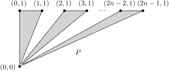
Figure 1. A star-shaped polygon $P$ with $\operatorname{b}(P)\geqslant\frac{1}{n}-\varepsilon$ and $\operatorname{c}(P)\leqslant\frac{1}{n}$. The polygon $P$ is a union of $n$ triangles $(0,0)(2i,1)(2i+1,1)$, $i=0,\dotsc,n-1$, and of a triangle $(0,0)(0,\delta)((2n-1)\delta,\delta)$, where $\delta$ is very small.

For weakly star-shaped polygons, Cabello et al. [6] showed that the above example is essentially optimal, providing the following linear upper bound on $\operatorname{b}(S)$.

Theorem 1.1 ([6, Theorem 5]).

For every weakly star-shaped simple polygon $P$, we have $\operatorname{b}(P)\leqslant 18\operatorname{c}(P)$.

For polygons that are not weakly star-shaped, Cabello et al. [6] gave a superlinear bound.

Theorem 1.2 ([6, Theorem 6]).

Every simple polygon $P$ satisfies

$$\operatorname{b}(P)\leqslant 12\operatorname{c}(P)\left(1+\log_{2}{\frac{1}{\operatorname{c}(P)}}\right).$$

Moreover, Cabello et al. [6] conjectured that even for a general simple polygon $P$, $\operatorname{b}(P)$ can be bounded from above by a linear function of $\operatorname{c}(P)$. (The question whether $\operatorname{b}(P)=O(\operatorname{c}(P))$ for simple polygons $P$ was originally asked by Cabello and Saumell [7].) The next theorem, which is the first main result of this paper, verifies this conjecture. Recall that $\operatorname{b}(S)$ is defined for a set $S$ if and only if $S$ has finite positive measure and $\operatorname{Seg}(S)$ is measurable. Recall also that a set is p-componentwise simply connected if its p-components are simply connected. In particular, every simply connected set is p-componentwise simply connected.

Theorem 1.3.

Every p-componentwise simply connected set $S\subseteq\mathbb{R}^{2}$ whose $\operatorname{b}(S)$ is defined satisfies $\operatorname{b}(S)\leqslant 180\operatorname{c}(S)$.

Clearly, every simple polygon satisfies the assumptions of Theorem 1.3. Hence we directly obtain the following, which verifies the conjecture of Cabello et al. [6].

Corollary 1.4.

Every simple polygon $P\subseteq\mathbb{R}^{2}$ satisfies $\operatorname{b}(P)\leqslant 180\operatorname{c}(P)$.

The main restriction in Theorem 1.3 is the assumption that $S$ is p-componentwise simply connected. This assumption cannot be omitted, as shown by the set $S\colonequals[0,1]^{2}\smallsetminus\mathbb{Q}^{2}$, where it is easy to verify that $\operatorname{c}(S)=0$ and $\operatorname{b}(S)=1$, see Proposition 3.7.

A related construction shows that Theorem 1.3 fails in higher dimensions. To see this, consider again the set $S\colonequals[0,1]^{2}\smallsetminus\mathbb{Q}^{2}$, and define a set $S^{\prime}\subseteq\mathbb{R}^{3}$ by

$$S^{\prime}\colonequals\{(tx,ty,t)\colon t\in[0,1]\text{ and }(x,y)\in S\}.$$

Again, it is easy to verify that $\operatorname{c}(S^{\prime})=0$ and $\operatorname{b}(S^{\prime})=1$, although $S^{\prime}$ is simply connected, even star-shaped.

Despite these examples, we will show that meaningful analogues of Theorem 1.3 for higher dimensions and for sets that are not p-componentwise simply connected are possible. The key is to use higher-order generalizations of the Beer index, which we introduce now.

For $k\in\{1,\dotsc,d\}$ and a set $S\subseteq\mathbb{R}^{d}$, we define the set $\operatorname{Simp}_{k}(S)\subseteq(\mathbb{R}^{d})^{k+1}$ by

$$\operatorname{Simp}_{k}(S)\colonequals\{(A_{0},\dotsc,A_{k})\in S^{k+1}\colon\operatorname{Conv}(\{A_{0},\dotsc,A_{k}\})\subseteq S\},$$

where the operator $\operatorname{Conv}$ denotes the convex hull of a set of points. We call $\operatorname{Simp}_{k}(S)$ the $k$-simplex set of $S$. Note that $\operatorname{Simp}_{1}(S)=\operatorname{Seg}(S)$.

For $k\in\{1,\dotsc,d\}$ and a set $S\subseteq\mathbb{R}^{d}$ with finite positive measure and with measurable $\operatorname{Simp}_{k}(S)$, we define $\operatorname{b}_{k}(S)$ by

$$\operatorname{b}_{k}(S)\colonequals\frac{\lambda_{(k+1)d}(\operatorname{Simp}_{k}(S))}{\lambda_{d}(S)^{k+1}}.$$

Note that $\operatorname{b}_{1}(S)=\operatorname{b}(S)$. We call $\operatorname{b}_{k}(S)$ the $k$-index of convexity of $S$. We again leave $\operatorname{b}_{k}(S)$ undefined if $S$ or $\operatorname{Simp}_{k}(S)$ is non-measurable, or if the measure of $S$ is not finite and positive.

We can view $\operatorname{b}_{k}(S)$ as the probability that the convex hull of $k+1$ points chosen from $S$ uniformly independently at random is contained in $S$. For any $S\subseteq\mathbb{R}^{d}$, we have $\operatorname{b}_{1}(S)\geqslant\operatorname{b}_{2}(S)\geqslant\dotsb\geqslant\operatorname{b}_{d}(S)$, provided all the $\operatorname{b}_{k}(S)$ are defined.

We remark that the set $S\colonequals[0,1]^{d}\smallsetminus\mathbb{Q}^{d}$ satisfies $\operatorname{c}(S)=0$ and $\operatorname{b}_{1}(S)=\operatorname{b}_{2}(S)=\dotsb=\operatorname{b}_{d-1}(S)=1$, see Proposition 3.7. Thus, for a general set $S\subseteq\mathbb{R}^{d}$, only the $d$-index of convexity can conceivably admit a nontrivial upper bound in terms of $\operatorname{c}(S)$. Our next result shows that such an upper bound on $\operatorname{b}_{d}(S)$ exists and is linear in $\operatorname{c}(S)$.

Theorem 1.5.

For every $d\geqslant 2$, there is a constant $\beta=\beta(d)>0$ such that every set $S\subseteq\mathbb{R}^{d}$ with $\operatorname{b}_{d}(S)$ defined satisfies $\operatorname{b}_{d}(S)\leqslant\beta\operatorname{c}(S)$.

We do not know if the linear upper bound in Theorem 1.5 is best possible. We can, however, construct examples showing that the bound is optimal up to a logarithmic factor. This is our last main result.

Theorem 1.6.

For every $d\geqslant 2$, there is a constant $\gamma=\gamma(d)>0$ such that for every $\varepsilon\in(0,1)$, there is a set $S\subseteq\mathbb{R}^{d}$ satisfying $\operatorname{c}(S)\leqslant\varepsilon$ and $\smash[b]{\operatorname{b}_{d}(S)\geqslant\gamma\frac{\varepsilon}{\log_{2}1/\varepsilon}}$, and in particular, we have $\operatorname{b}_{d}(S)\geqslant\gamma\frac{\operatorname{c}(S)}{\log_{2}1/\operatorname{c}(S)}$.

The proof of Theorem 1.3 is given in Section 2. In Section 3, we will prove Theorems 1.5 and 1.6. We conclude, in Section 4, with some further remarks and a collection of open problems.

2. Bounding the mutual visibility in the plane

The goal of this section is to prove Theorem 1.3. Since the proof is rather long and complicated, we first present a high-level overview of its main ideas.

We first show that it is sufficient to prove the estimate from Theorem 1.3 for bounded open simply connected sets. This is formalized by the next lemma, whose proof can be found in Section 2.2.

Lemma 2.1.

Let $\alpha>0$ be a constant such that every bounded open simply connected set $T\subseteq\mathbb{R}^{2}$ satisfies $\operatorname{b}(T)\leqslant\alpha\operatorname{c}(T)$. It follows that every p-componentwise simply connected set $S\subseteq\mathbb{R}^{2}$ with $\operatorname{b}(S)$ defined satisfies $\operatorname{b}(S)\leqslant\alpha\operatorname{c}(S)$.

In the proof of Lemma 2.1, we first show that the set $S$ can be reduced to a bounded open set $S^{\prime\prime}$ whose Beer index $\operatorname{b}(S^{\prime\prime})$ can be arbitrarily close to $\operatorname{b}(S)$ from below. This is done by considering a part $S^{\prime}$ of $S$ that is contained in a sufficiently large disc and by showing that all segments in $S^{\prime}$ are in fact contained in the interior of $S^{\prime}$, except for a set of measure zero. The proof is then finished by choosing $S^{\prime\prime}$ as the interior of $S^{\prime}$ and by applying the assumption of the lemma to every p-component of $S^{\prime\prime}$.

Suppose now that $S$ is a bounded open simply connected set. We seek a bound of the form $\operatorname{b}(S)=O(\operatorname{c}(S))$. This is equivalent to a bound of the form $\lambda_{4}(\operatorname{Seg}(S))=O(\operatorname{smc}(S)\lambda_{2}(S))$. We therefore need a suitable upper bound on $\lambda_{4}(\operatorname{Seg}(S))$.

We first choose in $S$ a diagonal $\ell$ (i.e., an inclusion-maximal line segment in $S$), and show that the set $S\smallsetminus\ell$ is a union of two open simply connected sets $S_{1}$ and $S_{2}$ (Lemma 2.4). It is not hard to show that the segments in $S$ that cross the diagonal $\ell$ contribute to $\lambda_{4}(\operatorname{Seg}(S))$ by at most $O(\operatorname{smc}(S)\lambda_{2}(S))$ (Lemma 2.8). Our main task is to bound the measure of $\operatorname{Seg}(S_{i}\cup\ell)$ for $i=1,2$. The two sets $S_{i}\cup\ell$ are what we call rooted sets. Informally, a rooted set is a union of a simply connected open set $S^{\prime}$ and an open segment $r\subseteq\partial S^{\prime}$, called the root.

To bound $\lambda_{4}(\operatorname{Seg}(R))$ for a rooted set $R$ with root $r$, we partition $R$ into levels $L_{1},L_{2},\dotsc$, where $L_{k}$ contains the points of $R$ that can be connected to $r$ by a polygonal line with $k$ segments, but not by a polygonal line with $k-1$ segments. Each segment in $R$ is contained in a union $L_{i}\cup L_{i+1}$ for some $i\geqslant 1$. Thus, a bound of the form $\lambda_{4}(\operatorname{Seg}(L_{i}\cup L_{i+1}))=O(\operatorname{smc}(R)\lambda_{2}(L_{i}\cup L_{i+1}))$ implies the required bound for $\lambda_{4}(\operatorname{Seg}(R))$.

We will show that each p-component of $L_{i}\cup L_{i+1}$ is a rooted set, with the extra property that all its points are reachable from its root by a polygonal line with at most two segments (Lemma 2.5). To handle such sets, we will generalize the techniques that Cabello et al. [6] have used to handle weakly star-shaped sets in their proof of Theorem 1.1. We will assign to every point $A\in R$ a set $\mathfrak{T}(A)$ of measure $O(\operatorname{smc}(R))$, such that for every $(A,B)\in\operatorname{Seg}(R)$, we have either $B\in\mathfrak{T}(A)$ or $A\in\mathfrak{T}(B)$ (Lemma 2.7). From this, Theorem 1.3 will follow easily.

2.1. Proof of Theorem 1.3 for bounded open simply connected sets

First, we need a few auxiliary lemmas.

Lemma 2.2.

For every positive integer $d$, if $S$ is an open subset of $\mathbb{R}^{d}$, then the set $\operatorname{Seg}(S)$ is open and the set $\operatorname{Vis}(A,S)$ is open for every point $A\in S$.

Proof.

Choose a pair of points $(A,B)\in\operatorname{Seg}(S)$. Since $S$ is open and $\overline{AB}$ is compact, there is $\varepsilon>0$ such that $\mathcal{N}_{\varepsilon}(\overline{AB})\subseteq S$. Consequently, for any $A^{\prime}\in\mathcal{N}_{\varepsilon}(A)$ and $B^{\prime}\in\mathcal{N}_{\varepsilon}(B)$, we have $\overline{A^{\prime}B^{\prime}}\subseteq S$, that is, $(A^{\prime},B^{\prime})\in\operatorname{Seg}(S)$. This shows that the set $\operatorname{Seg}(S)$ is open. If we fix $A^{\prime}=A$, then it follows that the set $\operatorname{Vis}(A,S)$ is open. ∎

Lemma 2.3.

Let $S$ be a simply connected subset of $\mathbb{R}^{2}$ and let $\ell$ and $\ell^{\prime}$ be line segments in $S$. It follows that the set $\operatorname{Vis}(\ell^{\prime},S)\cap\ell$ is a (possibly empty) subsegment of $\ell$.

Proof.

The statement is trivially true if $\ell$ and $\ell^{\prime}$ intersect or have the same supporting line, or if $\operatorname{Vis}(\ell^{\prime},S)\cap\ell$ is empty. Suppose that these situations do not occur. Let $A,B\in\ell$ and $A^{\prime},B^{\prime}\in\ell^{\prime}$ be such that $\overline{AA^{\prime}},\overline{BB^{\prime}}\subseteq S$. The points $A,A^{\prime},B^{\prime},B$ form a (possibly self-intersecting) tetragon $Q$ whose boundary is contained in $S$. Since $S$ is simply connected, the interior of $Q$ is contained in $S$. If $Q$ is not self-intersecting, then clearly $\overline{AB}\subseteq\operatorname{Vis}(\ell^{\prime},S)$. Otherwise, $\overline{AA^{\prime}}$ and $\overline{BB^{\prime}}$ have a point $D$ in common, and every point $C\in AB$ is visible in $R$ from the point $C^{\prime}\in A^{\prime}B^{\prime}$ such that $D\in\overline{CC^{\prime}}$. This shows that $\operatorname{Vis}(\ell^{\prime},S)\cap\ell$ is a convex subset and hence a subsegment of $\ell$. ∎

Now, we define rooted sets and their tree-structured decomposition, and we explain how they arise in the proof of Theorem 1.3.

A set $S\subseteq\mathbb{R}^{2}$ is half-open if every point $A\in S$ has a neighborhood $\mathcal{N}_{\varepsilon}(A)$ that satisfies one of the following two conditions:

1. $\mathcal{N}_{\varepsilon}(A)\subseteq S$,

2. $\mathcal{N}_{\varepsilon}(A)\cap\partial S$ is a diameter of $\mathcal{N}_{\varepsilon}(A)$ splitting it into two subsets, one of which (including the diameter) is $\mathcal{N}_{\varepsilon}(A)\cap S$ and the other (excluding the diameter) is $\mathcal{N}_{\varepsilon}(A)\smallsetminus S$.

The condition 1 holds for points $A\in{S}^{\circ}$, while the condition 2 holds for points $A\in\partial S$.

A set $R\subseteq\mathbb{R}^{2}$ is a rooted set if the following conditions are satisfied:

1. $R$ is bounded,

2. $R$ is p-connected and simply connected,

3. $R$ is half-open,

4. $R\cap\partial R$ is an open line segment.

The open line segment $R\cap\partial R$ is called the root of $R$. Every rooted set, as the union of a non-empty open set and an open line segment, is measurable and has positive measure.

A diagonal of a set $S\subseteq\mathbb{R}^{2}$ is a line segment contained in $S$ that is not a proper subset of any other line segment contained in $S$. Clearly, if $S$ is open, then every diagonal of $S$ is an open line segment. It is easy to see that the root of a rooted set $R$ is a diagonal of $R$.

The following lemma allows us to use a diagonal to split a bounded open simply connected subset of $\mathbb{R}^{2}$ into two rooted sets. It is intuitively clear, and its formal proof is postponed to Section 2.3.

Lemma 2.4.

Let $S$ be a bounded open simply connected subset of $\mathbb{R}^{2}$, and let $\ell$ be a diagonal of $S$. It follows that the set $S\smallsetminus\ell$ has two p-components $S_{1}$ and $S_{2}$. Moreover, $S_{1}\cup\ell$ and $S_{2}\cup\ell$ are rooted sets, and $\ell$ is their common root.

Let $R$ be a rooted set. For a positive integer $k$, the $k$th level $L_{k}$ of $R$ is the set of points of $R$ that can be connected to the root of $R$ by a polygonal line in $R$ consisting of $k$ segments but cannot be connected to the root of $R$ by a polygonal line in $R$ consisting of fewer than $k$ segments. We consider a degenerate one-vertex polygonal line as consisting of one degenerate segment, so the root of $R$ is part of $L_{1}$. Thus $L_{1}=\operatorname{Vis}(r,R)$, where $r$ denotes the root of $R$. A $k$-body of $R$ is a p-component of $L_{k}$. A body of $R$ is a $k$-body of $R$ for some $k$. See Figure 2 for an example of a rooted set and its partitioning into levels and bodies.

We say that a rooted set $P$ is attached to a set $Q\subseteq\mathbb{R}^{2}\smallsetminus P$ if the root of $P$ is subset of the interior of $P\cup Q$. The following lemma explains the structure of levels and bodies. Although it is intuitively clear, its formal proof requires quite a lot of work and can be found in Section 2.4.

Lemma 2.5.

Let $R$ be a rooted set and $(L_{k})_{k\geqslant 1}$ be its partition into levels. It follows that

1. $R=\bigcup_{k\geqslant 1}L_{k}$; consequently, $R$ is the union of all its bodies;

2. every body $P$ of $R$ is a rooted set such that $P=\operatorname{Vis}(r,P)$, where $r$ denotes the root of $P$;

3. $L_{1}$ is the unique $1$-body of $R$, and the root of $L_{1}$ is the root of $R$;

4. every $j$-body $P$ of $R$ with $j\geqslant 2$ is attached to a unique $(j-1)$-body of $R$.

Lemma 2.5 yields a tree structure on the bodies of $R$. The root of this tree is the unique $1$-body $L_{1}$ of $R$, called the root body of $R$. For a $k$-body $P$ of $R$ with $k\geqslant 2$, the parent of $P$ in the tree is the unique $(k-1)$-body of $R$ that $P$ is attached to, called the parent body of $P$.

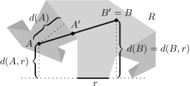
Figure 2. Example of a rooted set $R$ partitioned into six bodies. The three levels of $R$ are distinguished with three shades of gray. The segment $A^{\prime}B^{\prime}\cup\{B^{\prime}\}$ is the base segment of $\overline{AB}$.

Lemma 2.6.

Let $R$ be a rooted set, $(L_{k})_{k\geqslant 1}$ be the partition of $R$ into levels, $\ell$ be a closed line segment in $R$, and $k\geqslant 1$ be minimum such that $\ell\cap L_{k}\neq\emptyset$. It follows that $\ell\subseteq L_{k}\cup L_{k+1}$, $\ell\cap L_{k}$ is a subsegment of $\ell$ contained in a single $k$-body $P$ of $R$, and $\ell\cap L_{k+1}$ consists of at most two subsegments of $\ell$ each contained in a single $(k+1)$-body whose parent body is $P$.

Proof.

The definition of the levels directly yields $\ell\subseteq L_{k}\cup L_{k+1}$. The segment $\ell$ splits into subsegments each contained in a single $k$-body or $(k+1)$-body of $R$. By Lemma 2.5, the bodies of any two consecutive of these subsegments are in the parent-child relation of the body tree. This implies that $\ell\cap L_{k}$ lies within a single $k$-body $P$. By Lemma 2.3, $\ell\cap L_{k}$ is a subsegment of $\ell$. Consequently, $\ell\cap L_{k+1}$ consists of at most two subsegments. ∎

In the setting of Lemma 2.6, we call the subsegment $\ell\cap L_{k}$ of $\ell$ the base segment of $\ell$, and we call the body $P$ that contains $\ell\cap L_{k}$ the base body of $\ell$. See Figure 2 for an example.

The following lemma is the crucial part of the proof of Theorem 1.3.

Lemma 2.7.

If $R$ is a rooted set, then every point $A\in R$ can be assigned a measurable set $\mathfrak{T}(A)\subseteq\mathbb{R}^{2}$ so that the following is satisfied:

1. $\lambda_{2}(\mathfrak{T}(A))<87\operatorname{smc}(R)$;

2. for every line segment $\overline{BC}$ in $R$, we have either $B\in\mathfrak{T}(C)$ or $C\in\mathfrak{T}(B)$;

3. the set $\{(A,B)\colon A\in R$ and $B\in\mathfrak{T}(A)\}$ is measurable.

Proof.

Let $P$ be a body of $R$ with the root $r$. First, we show that $P$ is entirely contained in one closed half-plane defined by the supporting line of $r$. Let $h^{-}$ and $h^{+}$ be the two open half-planes defined by the supporting line of $r$. According to the definition of a rooted set, the sets $\{D\in r\colon\exists\varepsilon>0\colon\mathcal{N}_{\varepsilon}(D)\cap h^{-}=\mathcal{N}_{\varepsilon}(D)\cap(P\smallsetminus r)\}$ and $\{D\in r\colon\exists\varepsilon>0\colon\mathcal{N}_{\varepsilon}(D)\cap h^{+}=\mathcal{N}_{\varepsilon}(D)\cap(P\smallsetminus r)\}$ are open and partition the entire $r$, hence one of them must be empty. This implies that the segments connecting $r$ to $P\smallsetminus r$ lie all in $h^{-}$ or all in $h^{+}$. Since $P=\operatorname{Vis}(r,P)$, we conclude that $P\subseteq h^{-}$ or $P\subseteq h^{+}$.

According to the above, we can rotate and translate the set $R$ so that $r$ lies on the $x$-axis and $P$ lies in the half-plane $\{B\in\mathbb{R}^{2}\colon y(B)\geqslant 0\}$. For a point $A\in R$, we use $d(A,r)$ to denote the $y$-coordinate of $A$ after such a rotation and translation of $R$. We use $d(A)$ to denote $d(A,r)$ where $r$ is the root of the body of $A$. It follows that $d(A)\geqslant 0$ for every $A\in R$.

Let $\gamma\in(0,1)$ be a fixed constant whose value will be specified at the end of the proof. For a point $A\in R$, we define sets

$$\mathfrak{V}_{1}(A) \colonequals\{B\in\operatorname{Vis}(A,R)\colon|A^{\prime}B^{\prime}|\geqslant\gamma|AB|,\>A\in\operatorname{Vis}(r^{\prime\prime},R),\>d(A^{\prime},r^{\prime\prime})\geqslant d(B^{\prime},r^{\prime\prime})\},$$

$$\mathfrak{V}_{2}(A) \colonequals\{B\in\operatorname{Vis}(A,R)\colon|A^{\prime}B^{\prime}|\geqslant\gamma|AB|,\>A\notin\operatorname{Vis}(r^{\prime\prime},R),\>d(A^{\prime},r^{\prime\prime})\geqslant d(B^{\prime},r^{\prime\prime})\},$$

$$\mathfrak{V}_{3}(A) \colonequals\{B\in\operatorname{Vis}(A,R)\colon|A^{\prime}B^{\prime}|<\gamma|AB|,\>|AA^{\prime}|\geqslant|BB^{\prime}|\},$$

where $r^{\prime\prime}$ denotes the root of the base body of $\overline{AB}$ and $A^{\prime}$ and $B^{\prime}$ denote the endpoints of the base segment of $\overline{AB}$ such that $|AA^{\prime}|<|AB^{\prime}|$. For every $A\in R$, the sets $\mathfrak{V}_{1}(A)$, $\mathfrak{V}_{2}(A)$, and $\mathfrak{V}_{3}(A)$ are pairwise disjoint. Moreover, we have $A\in\bigcup_{i=1}^{3}\mathfrak{V}_{i}(B)$ or $B\in\bigcup_{i=1}^{3}\mathfrak{V}_{i}(A)$ for every line segment $\overline{AB}$ in $R$. If for some $B\in\bigcup_{i=1}^{3}\mathfrak{V}_{i}(A)$ the point $A$ lies on $r^{\prime\prime}$, then we have $B\in\mathfrak{V}_{1}(A)$ and $\mathfrak{V}_{1}(A)\subseteq r^{\prime\prime}$.

For the rest of the proof, we fix a point $A\in R$. We show that the union $\bigcup_{i=1}^{3}\mathfrak{V}_{i}(A)$ is contained in a measurable set $\mathfrak{T}(A)\subseteq\mathbb{R}^{2}$ with $\lambda_{2}(\mathfrak{T}(A))<87\operatorname{smc}(R)$ that is a union of three trapezoids. We let $P$ be the body of $A$ and $r$ be the root of $P$. If $P$ is a $k$-body with $k\geqslant 2$, then we use $r^{\prime}$ to denote the root of the parent body of $P$.

Claim 1.

$\mathfrak{V}_{1}(A)$ is contained in a trapezoid $\mathfrak{T}_{1}(A)$ with area $6\gamma^{-2}\operatorname{smc}(R)$.

Let $H$ be a point of $r$ such that $\overline{AH}\subseteq R$. Let $T^{\prime}$ be the $r$-parallel trapezoid of height $d(A)$ with bases of length $\smash[b]{\frac{8\operatorname{smc}(R)}{d(A)}}$ and $\smash[b]{\frac{4\operatorname{smc}(R)}{d(A)}}$ such that $A$ is the center of the larger base and $H$ is the center of the smaller base. The homothety with center $A$ and ratio $\gamma^{-1}$ transforms $T^{\prime}$ into the trapezoid $T\colonequals A+\gamma^{-1}(T^{\prime}-A)$. Since the area of $T^{\prime}$ is $6\operatorname{smc}(R)$, the area of $T$ is $6\gamma^{-2}\operatorname{smc}(R)$. We show that $\mathfrak{V}_{1}(A)\subseteq T$. See Figure 3 for an illustration.

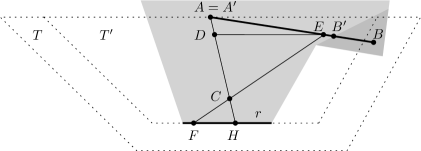
Figure 3. Illustration for the proof of Claim 1 in the proof of Lemma 2.7.

Let $B$ be a point in $\mathfrak{V}_{1}(A)$. Using a similar approach to the one used by Cabello et al. [6] in the proof of Theorem 1.1, we show that $B\in T$. Let $A^{\prime}B^{\prime}$ be the base segment of $\overline{AB}$ such that $|AA^{\prime}|<|AB^{\prime}|$. Since $B\in\mathfrak{V}_{1}(A)$, we have $|A^{\prime}B^{\prime}|\geqslant\gamma|AB|$, $A\in\operatorname{Vis}(r^{\prime\prime},R)$, and $d(B,r^{\prime\prime})\leqslant d(A,r^{\prime\prime})$, where $r^{\prime\prime}$ denotes the root of the base level of $\overline{AB}$. Since $A$ is visible from $r^{\prime\prime}$ in $R$, the base body of $\overline{AB}$ is the body of $A$ and thus $A=A^{\prime}$ and $r=r^{\prime\prime}$. As we have observed, every point $C\in\{A\}\cup AB^{\prime}$ satisfies $d(C,r)=d(C)\geqslant 0$.

Let $\varepsilon>0$. There is a point $E\in AB^{\prime}$ such that $|B^{\prime}E|<\varepsilon$. Since $E$ lies on the base segment of $\overline{AB}$, there is $F\in r$ such that $\overline{EF}\subseteq R$. It is possible to choose $F$ so that $\overline{AH}$ and $\overline{EF}$ have a point $C$ in common where $C\neq F,H$. Let $D$ be a point of $\overline{AH}$ with $d(D)=d(E)$. The point $D$ exists, as $d(H)=0\leqslant d(E)\leqslant d(A)$. The points $A,E,F,H$ form a self-intersecting tetragon $Q$ whose boundary is contained in $R$. Since $R$ is simply connected, the interior of $Q$ is contained in $R$ and the triangles $ACE$ and $CFH$ have area at most $\operatorname{smc}(R)$.

The triangle $ACE$ is partitioned into triangles $ADE$ and $CDE$ with areas $\frac{1}{2}(d(A)-d(D))|DE|$ and $\frac{1}{2}(d(D)-d(C))|DE|$, respectively. Therefore, we have $\frac{1}{2}(d(A)-d(C))|DE|=\lambda_{2}(ACE)\leqslant\operatorname{smc}(R)$. This implies

$$|DE|\leqslant\frac{2\operatorname{smc}(R)}{d(A)-d(C)}.$$

For the triangle $CFH$, we have $\frac{1}{2}d(C)|FH|=\lambda_{2}(CFH)\leqslant\operatorname{smc}(R)$. By the similarity of the triangles $CFH$ and $CDE$, we have $|FH|=|DE|d(C)/(d(E)-d(C))$ and therefore

$$|DE|\leqslant\frac{2\operatorname{smc}(R)}{d(C)^{2}}(d(E)-d(C)).$$

Since the first upper bound on $|DE|$ is increasing in $d(C)$ and the second is decreasing in $d(C)$, the minimum of the two is maximized when they are equal, that is, when $d(C)=d(A)d(E)/(d(A)+d(E))$. Then we obtain $|DE|\leqslant\smash[b]{\frac{2\operatorname{smc}(R)}{d(A)^{2}}}(d(A)+d(E))$. This and $0\leqslant d(E)\leqslant d(A)$ imply $E\in T^{\prime}$. Since $\varepsilon$ can be made arbitrarily small and $T^{\prime}$ is compact, we have $B^{\prime}\in T^{\prime}$. Since $|AB^{\prime}|\geqslant\gamma|AB|$, we conclude that $B\in T$. This completes the proof of Claim 1.

Claim 2.

$\mathfrak{V}_{2}(A)$ is contained in a trapezoid $\mathfrak{T}_{2}(A)$ with area $3(1-\gamma)^{-2}\gamma^{-2}\operatorname{smc}(R)$.

We assume the point $A$ is not contained in the first level of $R$, as otherwise $\mathfrak{V}_{2}(A)$ is empty. Let $p$ be the $r^{\prime}$-parallel line that contains the point $A$ and let $q$ be the supporting line of $r$. Let $p^{+}$ and $q^{+}$ denote the closed half-planes defined by $p$ and $q$, respectively, such that $r^{\prime}\subseteq p^{+}$ and $A\notin q^{+}$. Let $O$ be the intersection point of $p$ and $q$.

Let $T^{\prime}\subseteq p^{+}\cap q^{+}$ be the trapezoid of height $d(A,r^{\prime})$ with one base of length $\smash[b]{\frac{4\operatorname{smc}(R)}{(1-\gamma)^{2}d(A,r^{\prime})}}$ on $p$, the other base of length $\smash[b]{\frac{2\operatorname{smc}(R)}{(1-\gamma)^{2}d(A,r^{\prime})}}$ on the supporting line of $r^{\prime}$, and one lateral side on $q$. The homothety with center $O$ and ratio $\gamma^{-1}$ transforms $T^{\prime}$ into the trapezoid $T\colonequals O+\gamma^{-1}(T^{\prime}-O)$. Since the area of $T^{\prime}$ is $3(1-\gamma)^{-2}\operatorname{smc}(R)$, the area of $T$ is $3(1-\gamma)^{-2}\gamma^{-2}\operatorname{smc}(R)$. We show that $\mathfrak{V}_{2}(A)\subseteq T$. See Figure 4 for an illustration.

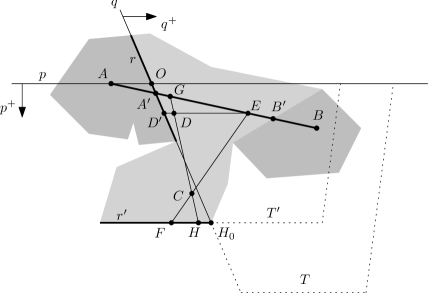
Figure 4. Illustration for the proof of Claim 2 in the proof of Lemma 2.7.

Let $B$ be a point of $\mathfrak{V}_{2}(A)$. We use $A^{\prime}B^{\prime}$ to denote the base segment of $\overline{AB}$ such that $|AA^{\prime}|<|AB^{\prime}|$. By the definition of $\mathfrak{V}_{2}(A)$, we have $|A^{\prime}B^{\prime}|\geqslant\gamma|AB|$, $A\notin\operatorname{Vis}(r^{\prime\prime},R)$, and $d(B,r^{\prime\prime})\leqslant d(A,r^{\prime\prime})$, where $r^{\prime\prime}$ denotes the root of the base body of $\overline{AB}$. By Lemma 2.6 and the fact that $A\notin\operatorname{Vis}(r^{\prime\prime},R)$, we have $r^{\prime}=r^{\prime\prime}$. The bound $d(A,r^{\prime})\geqslant d(B,r^{\prime})$ thus implies $A^{\prime}\in r\cap p^{+}$ and $B\in q^{+}$. We have $d(C,r^{\prime})=d(C)\geqslant 0$ for every $C\in A^{\prime}B^{\prime}$.

Observe that $(1-\gamma)d(A,r^{\prime})\leqslant d(A^{\prime},r^{\prime})\leqslant d(A,r^{\prime})$. The upper bound is trivial, as $d(B,r^{\prime})\leqslant d(A,r^{\prime})$ and $A^{\prime}$ lies on $\overline{AB}$. For the lower bound, we use the expression $A^{\prime}=tA+(1-t)B^{\prime}$ for some $t\in[0,1]$. This gives us $d(A^{\prime},r^{\prime})=td(A,r^{\prime})+(1-t)d(B^{\prime},r^{\prime})$. By the estimate $|A^{\prime}B^{\prime}|\geqslant\gamma|AB|$, we have

$$|AA^{\prime}|+|BB^{\prime}|\leqslant(1-\gamma)|AB|=(1-\gamma)(|AB^{\prime}|+|BB^{\prime}|).$$

This can be rewritten as $|AA^{\prime}|\leqslant(1-\gamma)|AB^{\prime}|-\gamma|BB^{\prime}|$. Consequently, $|BB^{\prime}|\geqslant 0$ and $\gamma>0$ imply $|AA^{\prime}|\leqslant(1-\gamma)|AB^{\prime}|$. This implies $t\geqslant 1-\gamma$. Applying the bound $d(B^{\prime},r^{\prime})\geqslant 0$, we conclude that $d(A^{\prime},r^{\prime})\geqslant(1-\gamma)d(A,r^{\prime})$.

Let $(G_{n})_{n\in\mathbb{N}}$ be a sequence of points from $A^{\prime}B^{\prime}$ that converges to $A^{\prime}$. For every $n\in\mathbb{N}$, there is a point $H_{n}\in r^{\prime}$ such that $\overline{G_{n}H_{n}}\subseteq R$. Since $\overline{r^{\prime}}$ is compact, there is a subsequence of $(H_{n})_{n\in\mathbb{N}}$ that converges to a point $H_{0}\in\overline{r^{\prime}}$. We claim that $H_{0}\in q$. Suppose otherwise, and let $q^{\prime}\neq q$ be the supporting line of $\overline{A^{\prime}H_{0}}$. Let $\varepsilon>0$ be small enough so that $\mathcal{N}_{\varepsilon}(A^{\prime})\subseteq R$. For $n$ large enough, $\overline{G_{n}H_{n}}$ is contained in an arbitrarily small neighborhood of $q^{\prime}$. Consequently, for $n$ large enough, the supporting line of $\overline{G_{n}H_{n}}$ intersects $q$ at a point $K_{n}$ such that $\overline{G_{n}K_{n}}\subseteq\mathcal{N}_{\varepsilon}(A^{\prime})$, which implies $K_{n}\in r\cap\operatorname{Vis}(r^{\prime},R)$, a contradiction.

Again, let $\varepsilon>0$. There is a point $E\in A^{\prime}B^{\prime}$ such that $|B^{\prime}E|<\varepsilon$. Let $D^{\prime}$ be a point of $q$ with $d(D^{\prime},r^{\prime})=d(E)$, and let $\delta>0$. There are points $G\in A^{\prime}B^{\prime}$ and $H\in r^{\prime}$ such that $G\in\mathcal{N}_{\delta}(A^{\prime})$ and $\overline{GH}\subseteq R\cap\mathcal{N}_{\delta}(q)$. If $\delta$ is small enough, then $d(E)\leqslant d(A^{\prime},r^{\prime})-\delta\leqslant d(G)\leqslant d(A^{\prime},r^{\prime})$. Let $D$ be the point of $\overline{GH}$ with $d(D)=d(E)$. The point $E$ lies on $A^{\prime}B^{\prime}$ and thus it is visible from a point $F\in r^{\prime}$. Again, we can choose $F$ so that the line segments $\overline{EF}$ and $\overline{GH}$ have a point $C$ in common where $C\neq F,H$. The points $E,F,H,G$ form a self-intersecting tetragon $Q$ whose boundary is in $R$. The interior of $Q$ is contained in $R$, as $R$ is simply connected. Therefore, the area of the triangles $CEG$ and $CFH$ is at most $\operatorname{smc}(R)$.

The argument used in the proof of Claim 1 yields

$$|DE|\leqslant\frac{2\operatorname{smc}(R)}{d(G)^{2}}(d(G)+d(E))\leqslant\frac{2\operatorname{smc}(R)}{(d(A^{\prime},r^{\prime})-\delta)^{2}}(d(A^{\prime},r^{\prime})+d(E)).$$

This and the fact that $\delta$ (and consequently $|D^{\prime}D|$) can be made arbitrarily small yield $|D^{\prime}E|\leqslant\frac{2\operatorname{smc}(R)}{d(A^{\prime},r^{\prime})^{2}}(d(A^{\prime},r^{\prime})+d(E))$. This and $d(A^{\prime},r^{\prime})\geqslant(1-\gamma)d(A,r^{\prime})$ yield $|D^{\prime}E|\leqslant\frac{2\operatorname{smc}(R)}{(1-\gamma)^{2}d(A,r^{\prime})^{2}}(d(A,r^{\prime})+d(E))$. This and $0\leqslant d(E)\leqslant d(A)$ imply $E\in T^{\prime}$.

Since $\varepsilon$ can be made arbitrarily small and $T^{\prime}$ is compact, we have $B^{\prime}\in T^{\prime}$. Since $|A^{\prime}B^{\prime}|\geqslant\gamma|AB|\geqslant\gamma|A^{\prime}B|$, we conclude that $B\in T$. This completes the proof of Claim 2.

Claim 3.

$\mathfrak{V}_{3}(A)$ is contained in a trapezoid $\mathfrak{T}_{3}(A)$ with area $(4(1-\gamma)^{-2}-1)\operatorname{smc}(R)$.

By Lemma 2.3, the points of $r$ that are visible from $A$ in $R$ form a subsegment $CD$ of $r$. The homothety with center $A$ and ratio $2(1-\gamma)^{-1}$ transforms the triangle $T^{\prime}\colonequals ACD$ into the triangle $T^{\prime\prime}\colonequals A+2(1-\gamma)^{-1}(T^{\prime}-A)$. See Figure 5 for an illustration. We claim that $\mathfrak{V}_{3}(A)$ is a subset of the trapezoid $T\colonequals T^{\prime\prime}\smallsetminus T^{\prime}$.

Let $B$ be an arbitrary point of $\mathfrak{V}_{3}(A)$. Consider the segment $\overline{AB}$ with the base segment $A^{\prime}B^{\prime}$ such that $|AA^{\prime}|<|AB^{\prime}|$. Since $B\in\mathfrak{V}_{3}(A)$, we have $|A^{\prime}B^{\prime}|<\gamma|AB|$ and $|AA^{\prime}|\geqslant|BB^{\prime}|$. This implies $|AA^{\prime}|\geqslant\frac{1-\gamma}{2}|AB|>0$ and hence $A\neq A^{\prime}$ and $B\notin P$. From the definition of $C$ and $D$, we have $A^{\prime}\in\overline{CD}$. Since $|AA^{\prime}|\geqslant\frac{1-\gamma}{2}|AB|$ and $B\notin P$, we have $B\in T$.

The area of $T$ is $(4(1-\gamma)^{-2}-1)\lambda_{2}(T^{\prime})$. The interior of $T^{\prime}$ is contained in $R$, as all points of the open segment $CD$ are visible from $A$ in $R$. The area of $T^{\prime}$ is at most $\operatorname{smc}(R)$, as its interior is a convex subset of $R$. Consequently, the area of $T$ is at most $(4(1-\gamma)^{-2}-1)\operatorname{smc}(R)$. This completes the proof of Claim 3.

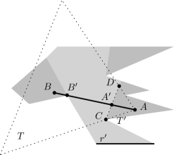
Figure 5. Illustration for the proof of Claim 3 in the proof of Lemma 2.7.

To put everything together, we set $\mathfrak{T}(A)\colonequals\bigcup_{i=1}^{3}\mathfrak{T}_{i}(A)$. Then, it follows that $\bigcup_{i=1}^{3}\mathfrak{V}_{i}(A)\subseteq\mathfrak{T}(A)$ for every $A\in R$. Clearly, the set $\mathfrak{T}(A)$ is measurable. Summing the three estimates on areas of the trapezoids, we obtain

$$\lambda_{2}(\mathfrak{T}(A))\leqslant\bigl{(}6\gamma^{-2}+3(1-\gamma)^{-2}\gamma^{-2}+4(1-\gamma)^{-2}-1\bigr{)}\operatorname{smc}(R)$$

for every point $A\in R$. We choose $\gamma\in(0,1)$ so that the value of the coefficient is minimized. For $x\in(0,1)$, the function $x\mapsto 6x^{-2}+3(1-x)^{-2}x^{-2}+4(1-x)^{-2}-1$ attains its minimum $86.7027<87$ at $x\approx 0.5186$. Altogether, we have $\lambda_{2}(\mathfrak{T}(A))<87\operatorname{smc}(R)$ for every $A\in R$.

It remains to show that the set $\{(A,B)\colon A\in R$ and $B\in\mathfrak{T}(A)\}$ is measurable. For every body $P$ of $R$ and for $i\in\{1,2,3\}$, the definition of the trapezoid $\mathfrak{T}_{i}(A)$ in Claim $i$ implies that the set $\{(A,B)\colon A\in P$ and $B\in\mathfrak{T}_{i}(A)\}$ is the intersection of $P\times\mathbb{R}^{2}$ with a semialgebraic (hence measurable) subset of $(\mathbb{R}^{2})^{2}$ and hence is measurable. There are countably many bodies of $R$, as each of them has positive measure. Therefore, $\{(A,B)\colon A\in R$ and $B\in\mathfrak{T}(A)\}$ is a countable union of measurable sets and hence is measurable. ∎

Let $S$ be a bounded open subset of the plane, and let $\ell$ be a diagonal of $S$ that lies on the $x$-axis. For a point $A\in S$, we define the set

$$\mathfrak{S}(A,\ell)\colonequals\{B\in\operatorname{Vis}(A,S)\colon AB\cap\ell\neq\emptyset\text{ and }|y(A)|\geqslant|y(B)|\}.$$

The following lemma is a slightly more general version of a result of Cabello et al. [6].

Lemma 2.8.

Let $S$ be a bounded open simply connected subset of $\mathbb{R}^{2}$, and let $\ell$ be its diagonal. It follows that $\lambda_{2}(\mathfrak{S}(A,\ell))\leqslant 3\operatorname{smc}(S)$ for every $A\in S$.

Proof.

We can assume without loss of generality that $\ell$ lies on the $x$-axis. Using an argument similar to the proof of Lemma 2.2, we can show that the set $\{B\in\operatorname{Vis}(A,S)\colon AB\cap\ell\neq\emptyset\}$ is open. Therefore, $\mathfrak{S}(A,\ell)$ is the intersection of an open set and the closed half-plane $\{(x,y)\in\mathbb{R}^{2}\colon y\leqslant-y(A)\}$ or $\{(x,y)\in\mathbb{R}^{2}\colon y\geqslant-y(A)\}$, whichever contains $A$. Consequently, the set $\mathfrak{S}(A,\ell)$ is measurable for every $A\in S$.

We clearly have $\lambda_{2}(\mathfrak{S}(A,\ell))=0$ for points $A\in S\smallsetminus\operatorname{Vis}(\ell,S)$. By Lemma 2.3, the set $\operatorname{Vis}(A,S)\cap\ell$ is an open subsegment $CD$ of $\ell$. The interior ${T}^{\circ}$ of the triangle $T\colonequals ACD$ is contained in $S$. Since ${T}^{\circ}$ is a convex subset of $S$, we have $\lambda_{2}({T}^{\circ})=\frac{1}{2}|CD|\cdot|y(A)|\leqslant\operatorname{smc}(S)$. Therefore, every point $B\in\mathfrak{S}(A,\ell)$ is contained in a trapezoid of height $|y(A)|$ with bases of length $|CD|$ and $2|CD|$. The area of this trapezoid is $\frac{3}{2}|CD|\cdot|y(A)|\leqslant 3\operatorname{smc}(S)$. Hence we have $\lambda_{2}(\mathfrak{S}(A,\ell))\leqslant 3\operatorname{smc}(S)$ for every point $A\in S$. ∎

Proof of Theorem 1.3.

In view of Lemma 2.1, we can assume without loss of generality that $S$ is a bounded open simply connected set. Let $\ell$ be a diagonal of $S$. We can assume without loss of generality that $\ell$ lies on the $x$-axis.

According to Lemma 2.4, the set $S\smallsetminus\ell$ has exactly two p-components $S_{1}$ and $S_{2}$, the sets $S_{1}\cup\ell$ and $S_{2}\cup\ell$ are rooted sets, and $\ell$ is their common root. By Lemma 2.7, for $i\in\{1,2\}$, every point $A\in S_{i}\cup\ell$ can be assigned a measurable set $\mathfrak{T}_{i}(A)$ so that $\lambda_{2}(\mathfrak{T}_{i}(A))<87\operatorname{smc}(S_{i}\cup\ell)\leqslant 87\operatorname{smc}(S)$, every line segment $\overline{BC}$ in $S_{i}\cup\ell$ satisfies $B\in\mathfrak{T}_{i}(C)$ or $C\in\mathfrak{T}_{i}(B)$, and the set $\{(A,B)\colon A\in S_{i}\cup\ell$ and $B\in\mathfrak{T}_{i}(A)\}$ is measurable.

We set $\mathfrak{S}(A)\colonequals\mathfrak{T}_{i}(A)\cup\mathfrak{S}(A,\ell)$ for every point $A\in S_{i}$ with $i\in\{1,2\}$. We set $\mathfrak{S}(A)\colonequals\mathfrak{T}_{1}(A)\cup\mathfrak{T}_{2}(A)$ for every point $A\in\ell=S\smallsetminus(S_{1}\cup S_{2})$. Let

$$\mathfrak{S}\colonequals\{(A,B)\colon A\in S\text{ and }B\in\mathfrak{S}(A)\}\cup\{(B,A)\colon A\in S\text{ and }B\in\mathfrak{S}(A)\}\subseteq(\mathbb{R}^{2})^{2}.$$

It follows that the set $\mathfrak{S}$ is measurable.

Let $\overline{AB}$ be a line segment in $S$, and suppose $|y(A)|\geqslant|y(B)|$. Then either $A$ and $B$ are in distinct p-components of $S\smallsetminus\ell$ or they both lie in the same component $S_{i}$ with $i\in\{1,2\}$. In the first case, we have $B\in\mathfrak{S}(A)$, since $AB$ intersects $\ell$ and $\mathfrak{S}(A,\ell)\subseteq\mathfrak{S}(A)$. In the second case, we have $B\in\mathfrak{T}_{i}(A)\subseteq\mathfrak{S}(A)$ or $A\in\mathfrak{T}_{i}(B)\subseteq\mathfrak{S}(B)$. Therefore, we have $\operatorname{Seg}(S)\subseteq\mathfrak{S}$. Since both $\operatorname{Seg}(S)$ and $\mathfrak{S}$ are measurable, we have

$$\lambda_{4}(\operatorname{Seg}(S))\leqslant\lambda_{4}(\mathfrak{S})\leqslant 2\int_{A\in S}\lambda_{2}(\mathfrak{S}(A)),$$

where the second inequality is implied by Fubini’s Theorem. The bound $\lambda_{2}(\mathfrak{S}(A))\leqslant 90\operatorname{smc}(S)$ implies

$$\lambda_{4}(\operatorname{Seg}(S))\leqslant 2\int_{S}90\operatorname{smc}(S)=180\operatorname{smc}(S)\lambda_{2}(S).$$

Finally, this bound can be rewritten as $\operatorname{b}(S)=\lambda_{4}(\operatorname{Seg}(S))\lambda_{2}(S)^{-2}\leqslant 180\operatorname{c}(S)$. ∎

2.2. Proof of Lemma 2.1

In this section, we prove Lemma 2.1, which reduces the general setting of Theorem 1.3 to the case that $S$ is a bounded open simply connected subset of $\mathbb{R}^{2}$.

Lemma 2.9.

Let $S\subseteq\mathbb{R}^{2}$ be a set whose $\operatorname{b}(S)$ is defined. For every $\varepsilon>0$, there is a bounded set $S^{\prime}\subseteq S$ such that $\lambda(S^{\prime})\geqslant(1-\varepsilon)\lambda(S)$ and $\operatorname{b}(S^{\prime})\geqslant\operatorname{b}(S)-\varepsilon$. Moreover, if $S$ is p-componentwise simply connected, then so is $S^{\prime}$.

Proof.

Let $B$ be an open ball in $\mathbb{R}^{2}$ centered at the origin. Consider the sets $S^{\prime}=S\cap B$ and $S_{0}=S\smallsetminus B$ partitioning the set $S$. Fix the radius of $B$ large enough, so that $S_{0}$ has measure at most $\varepsilon\lambda(S)/2$. We claim that $S^{\prime}$ has the properties stated in the lemma.

Clearly $\lambda(S^{\prime})\geqslant(1-\varepsilon/2)\lambda(S)>(1-\varepsilon)\lambda(S)$. Moreover, $\operatorname{Seg}(S^{\prime})=\operatorname{Seg}(S)\smallsetminus((S_{0}\times S)\cup(S\times S_{0}))$, and hence $\operatorname{Seg}(S^{\prime})$ is measurable and we have $\lambda_{4}(\operatorname{Seg}(S^{\prime}))\geqslant\lambda_{4}(\operatorname{Seg}(S))-\varepsilon\lambda(S)^{2}$. Therefore,

$$\operatorname{b}(S^{\prime})=\frac{\lambda_{4}(\operatorname{Seg}(S^{\prime}))}{\lambda_{4}(S^{\prime}\times S^{\prime})}\geqslant\frac{\lambda_{4}(\operatorname{Seg}(S^{\prime}))}{\lambda_{4}(S\times S)}\geqslant\frac{\lambda_{4}(\operatorname{Seg}(S))-\varepsilon\lambda(S)^{2}}{\lambda_{4}(S\times S)}=\operatorname{b}(S)-\varepsilon,$$

as claimed. It is clear from the construction that if $S$ is p-componentwise simply connected, then so is $S^{\prime}$. ∎

Lemma 2.10.

Let $S\subseteq\mathbb{R}^{2}$ be a bounded p-componentwise simply connected measurable set with measurable segment set. Then $\lambda_{4}(\operatorname{Seg}(S)\smallsetminus\operatorname{Seg}({S}^{\circ}))=0$. In other words, all the segments in $S$ are in fact contained in ${S}^{\circ}$, except for a set of measure zero.

Proof.

Let $\mathfrak{B}$ denote the set $\operatorname{Seg}(S)\smallsetminus\operatorname{Seg}({S}^{\circ})$, that is, $\mathfrak{B}$ is the set of segments in $S$ containing at least one point of $\partial S$. Note that $\mathfrak{B}$ is measurable, since $\operatorname{Seg}(S)$ is measurable by assumption and $\operatorname{Seg}({S}^{\circ})$ is an open set by Lemma 2.2, hence it is measurable as well.

Let $\overline{AB}$ be a segment contained in $S$, and let $C$ be a point of $\overline{AB}$. We say that $C$ is an isolated boundary point of the segment $\overline{AB}$, if $C\in\partial S$, but there is an $\varepsilon>0$ such that no other point of $\overline{AB}\cap\mathcal{N}_{\varepsilon}(C)$ belongs to $\partial S$.

We partition the set $\mathfrak{B}$ into four parts as follows:

$$\mathfrak{B}_{|} \colonequals\{(A,B)\in\mathfrak{B}\colon A=B\text{ or }\overline{AB}\text{ is a vertical segment}\},$$

$$\mathfrak{B}_{\lhd} \colonequals\{(A,B)\in\mathfrak{B}\smallsetminus\mathfrak{B}_{|}\colon A\text{ is an isolated boundary point of }\overline{AB}\},$$

$$\mathfrak{B}_{\rhd} \colonequals\{(A,B)\in\mathfrak{B}\smallsetminus(\mathfrak{B}_{|}\cup\mathfrak{B}_{\lhd})\colon B\text{ is an isolated boundary point of }\overline{AB}\},$$

$$\mathfrak{B}_{\bullet} \colonequals\mathfrak{B}\smallsetminus(\mathfrak{B}_{|}\cup\mathfrak{B}_{\lhd}\cup\mathfrak{B}_{\rhd}).$$

We claim that each of these sets has measure zero. For $\mathfrak{B}_{|}$, this is clear, since $\mathfrak{B}_{|}$ is a subset of $\{(A,B)\in\mathbb{R}^{2}\times\mathbb{R}^{2}\colon A=B\text{ or }\overline{AB}\text{ is a vertical segment}\}$, which clearly has $\lambda_{4}$-measure zero.

Consider now the set $\mathfrak{B}_{\lhd}$. We first argue that it is measurable. For a set $\alpha\subseteq[0,1]$ and a pair of points $(A,B)$, define $\overline{AB}[\alpha]\colonequals\{tB+(1-t)A\colon t\in\alpha\}$, and let $\mathfrak{S}(\alpha)$ be the set $\{(A,B)\in\mathbb{R}^{2}\times\mathbb{R}^{2}\colon\overline{AB}[\alpha]\subseteq{S}^{\circ}\}$. In particular, if $\alpha=[0,1]$ then $\overline{AB}[\alpha]=\overline{AB}$ and $\mathfrak{S}(\alpha)=\operatorname{Seg}({S}^{\circ})$. If $\alpha$ is a closed interval, then $\overline{AB}[\alpha]$ is a segment, and it is not hard to see that $\mathfrak{S}(\alpha)$ is an open set, and, in particular, it is measurable. If $\alpha$ is an open interval, say $\alpha=(s,t)\subseteq[0,1]$, then $\mathfrak{S}(\alpha)=\bigcap_{n\in\mathbb{N}}\mathfrak{S}([s+n^{-1},t-n^{-1}])$, and hence $\mathfrak{S}(\alpha)$ is measurable as well. We then see that

$$\mathfrak{B}_{\lhd}=\mathfrak{B}\cap(\partial{S}\times S)\cap\Bigl{(}\bigcup_{n\in\mathbb{N}}\mathfrak{S}((0,n^{-1}))\Bigr{)},$$

showing that $\mathfrak{B}_{\lhd}$ is measurable. An analogous argument shows that $\mathfrak{B}_{\rhd}$ is measurable, and hence $\mathfrak{B}_{\bullet}$ is measurable as well.

In the rest of the proof, we will use two basic facts of integral calculus, which we now state explicitly.

Fact 1 (see [18, Lemma 7.25 and Theorem 7.26]).

Let $X,Y\subseteq\mathbb{R}^{d}$ be two open sets, and let $\sigma\colon X\to Y$ be a bijection such that both $\sigma$ and $\sigma^{-1}$ are continuous and differentiable on $X$ and $Y$, respectively. Then, for any $X_{0}\subseteq X$, the set $X_{0}$ is measurable if and only if $\sigma(X_{0})$ is measurable. Moreover, $\lambda(X_{0})=0$ if and only if $\lambda(\sigma(X_{0}))=0$.

Fact 2 (Fubini’s Theorem, see [18, Theorem 8.12]).

Let $M\subseteq\mathbb{R}^{k}\times\mathbb{R}^{\ell}$ be a measurable set. For $x\in\mathbb{R}^{k}$, define $M_{x}\colonequals\{y\in\mathbb{R}^{\ell}\colon(x,y)\in M\}$. Then, for almost every $x\in\mathbb{R}^{k}$, the set $M_{x}$ is $\lambda_{\ell}$-measurable, and

$$\lambda_{k+\ell}(M)=\int_{x\in\mathbb{R}^{k}}\lambda_{\ell}(M_{x}).$$

Let us prove that $\lambda_{4}(\mathfrak{B}_{\lhd})=0$. The basic idea is as follows: suppose that we have fixed a non-vertical line $L$ and a point $B\in L$. It can be easily seen that there are at most countably many points $A\in L$ such that $(A,B)\in\mathfrak{B}_{\lhd}$. Since a line $L$ with a point $B\in L$ can be determined by three parameters, we will see that $\mathfrak{B}_{\lhd}$ has $\lambda_{4}$-measure zero.

Let us describe this reasoning more rigorously. Let $L_{a,b}$ denote the line $\{(x,y)\in\mathbb{R}^{2}\colon y=ax+b\}$. Define a mapping $\sigma\colon\mathbb{R}^{4}\to\mathbb{R}^{2}\times\mathbb{R}^{2}$ as follows: $\sigma(a,b,x,x^{\prime})=(A,B)$, where $A=(x,ax+b)$ and $B=(x^{\prime},ax^{\prime}+b)$. In other words, $\sigma(a,b,x,x^{\prime})$ is the pair of points on the line $L_{a,b}$ whose horizontal coordinates are $x$ and $x^{\prime}$, respectively. For every non-vertical segment $\overline{AB}$, there is a unique quadruple $(a,b,x,x^{\prime})$ with $x\neq x^{\prime}$, such that $\sigma(a,b,x,x^{\prime})=(A,B)$. In particular, $\sigma$ is a bijection from the set $\{(a,b,x,x^{\prime})\in\mathbb{R}^{4}\colon x\neq x^{\prime}\}$ to the set $\{(A,B)\in\mathbb{R}^{2}\times\mathbb{R}^{2}\colon A,B$ not on the same vertical line$\}$.

Define $\widehat{\mathfrak{B}}_{\lhd}=\sigma^{-1}(\mathfrak{B}_{\lhd})$. Note that $\sigma$ satisfies the assumptions of Fact 1, and therefore $\widehat{\mathfrak{B}}_{\lhd}$ is measurable. Moreover, $\lambda_{4}(\widehat{\mathfrak{B}}_{\lhd})=0$ if and only if $\lambda_{4}(\mathfrak{B}_{\lhd})=0$.

For a fixed triple $(a,b,x^{\prime})\in\mathbb{R}^{3}$, let $X_{a,b,x^{\prime}}$ denote the set $\{x\in\mathbb{R}\colon(a,b,x,x^{\prime})\in\widehat{\mathfrak{B}}_{\lhd}\}$. We claim that $X_{a,b,x^{\prime}}$ is countable. To see this, choose a point $x\in X_{a,b,x^{\prime}}$ and define $(A,B)\colonequals\sigma(a,b,x,x^{\prime})$. Since $(A,B)\in\mathfrak{B}_{\lhd}$, we know that $A$ is an isolated boundary point of $\overline{AB}$, which implies that there is a closed interval $\beta\subseteq\mathbb{R}$ of positive length such that $\beta\cap X_{a,b,x^{\prime}}=\{x\}$. This implies that $X_{a,b,x^{\prime}}$ is countable and thus of measure zero.

Since $\widehat{\mathfrak{B}}_{\lhd}$ is measurable, we can apply Fubini’s Theorem to get

$$\lambda_{4}(\widehat{\mathfrak{B}}_{\lhd})=\int_{(a,b,x^{\prime})\in\mathbb{R}^{3}}\lambda_{1}(X_{a,b,x^{\prime}}).$$

Therefore $\lambda_{4}(\widehat{\mathfrak{B}}_{\lhd})=0$ as claimed. A similar argument shows that $\lambda_{4}(\widehat{\mathfrak{B}}_{\rhd})=0$.

It remains to deal with the set $\mathfrak{B}_{\bullet}$. We will use the following strategy: we will fix two parallel non-horizontal lines $L_{1},L_{2}$, and study the segments orthogonal to these two lines, with one endpoint on $L_{1}$ and the other on $L_{2}$. Roughly speaking, our goal is to show that for “almost every” choice of $L_{1}$ and $L_{2}$, there are “almost no” segments of this form belonging to $\mathfrak{B}_{\bullet}$.

Let $L^{\prime}_{a,b}$ denote the (non-horizontal) line $\{(ay+b,y)\colon y\in\mathbb{R}\}$. Let us say that a pair of distinct points $(A,B)$ has type $(a,b,c)$, if $A\in L^{\prime}_{a,b}$, $B\in L^{\prime}_{a,c}$, and the segment $\overline{AB}$ is orthogonal to $L^{\prime}_{a,b}$ (and therefore also to $L^{\prime}_{a,c}$). The value $a$ is then called the slope of the type $t=(a,b,c)$.

Note that every pair of distinct points $(A,B)$ defining a non-vertical segment has a unique type $(a,b,c)$, with $b\neq c$. Define a mapping $\tau\colon\mathbb{R}^{4}\to\mathbb{R}^{2}\times\mathbb{R}^{2}$, where $\tau(a,b,c,y)$ is the pair of points $(A,B)$ of type $(a,b,c)$ such that $A=(ay+b,y)$. Note that $\tau$ is a bijection from the set $\{(a,b,c,y)\in\mathbb{R}^{4}\colon b\neq c\}$ to the set $\{(A,B)\in\mathbb{R}^{2}\times\mathbb{R}^{2}\colon A,B$ not on the same vertical line$\}$. We can easily verify that $\tau$ satisfies the assumptions of Fact 1.

Define $\widetilde{\mathfrak{B}}_{\bullet}=\tau^{-1}(\mathfrak{B}_{\bullet})$. From Fact 1, it follows that $\widetilde{\mathfrak{B}}_{\bullet}$ is measurable, and $\lambda_{4}(\mathfrak{B}_{\bullet})=0$ if and only if $\lambda_{4}(\widetilde{\mathfrak{B}}_{\bullet})=0$. For a type $t=(a,b,c)\in\mathbb{R}^{3}$, define $Y_{t}=\{y\in\mathbb{R}\colon(a,b,c,y)\in\widetilde{\mathfrak{B}}_{\bullet}\}$. Furthermore, for a set $\alpha\subseteq[0,1]$, define $\mathfrak{B}_{\bullet}(\alpha)=\mathfrak{B}_{\bullet}\cap\mathfrak{S}(\alpha)$, $\widetilde{\mathfrak{B}}_{\bullet}(\alpha)=\tau^{-1}(\mathfrak{B}_{\bullet}(\alpha))$, and $Y_{t}(\alpha)=\{y\in\mathbb{R}\colon(a,b,c,y)\in\widetilde{\mathfrak{B}}_{\bullet}(\alpha)\}$. In our applications, $\alpha$ will always be an interval (in fact, an open interval with rational endpoints), and in such case we already know that $\mathfrak{B}_{\bullet}(\alpha)$ is measurable, hence $\widetilde{\mathfrak{B}}_{\bullet}(\alpha)$ is measurable.

By Fubini’s Theorem, we have

($$* \lambda_{4}(\widetilde{\mathfrak{B}}_{\bullet})=\int_{a\in\mathbb{R}}\int_{(b,c)\in\mathbb{R}^{2}}\lambda_{1}(Y_{(a,b,c)}),$$)

and $Y_{t}$ is measurable for all $t\in\mathbb{R}^{3}$ up to a set of $\lambda_{3}$-measure zero. An analogous formula holds for $\widetilde{\mathfrak{B}}_{\bullet}(\alpha)$ and $Y_{t}(\alpha)$ for any open interval $\alpha\subseteq[0,1]$ with rational endpoints. Since there are only countably many such intervals, and a countable union of sets of measure zero has measure zero, we know that there is a set $T_{0}\subseteq\mathbb{R}^{3}$ of measure zero, such that for all $t\in\mathbb{R}^{3}\smallsetminus T_{0}$ the set $Y_{t}$ is measurable, and moreover for any rational interval $\alpha$ the set $Y_{t}(\alpha)$ is measurable as well.

Our goal is to show that there are at most countably many slopes $a\in\mathbb{R}$ for which there is a $(b,c)\in\mathbb{R}^{2}$ such that $\lambda_{1}(Y_{(a,b,c)})>0$. From ($*$ ‣ 2.2) it will then follow that $\widetilde{\lambda}_{4}(\mathfrak{B}_{\bullet})=0$. To achieve this goal, we will show that to any type $t$ for which $\lambda_{1}(Y_{t})>0$, we can assign a set $R_{t}\subseteq\partial S$ of positive $\lambda_{2}$-measure (the region of $t$), so that if $t$ and $t^{\prime}$ have different slopes and if $Y_{t}$ and $Y_{t^{\prime}}$ both have positive measure, then $R_{t}$ and $R_{t^{\prime}}$ are disjoint. Since there cannot be uncountably many disjoint sets of positive measure, this will imply the result.

Let us fix a type $t=(a,b,c)\in\mathbb{R}^{3}\smallsetminus T_{0}$ such that $\lambda_{1}(Y_{t})>0$. Let us say that an element $y\in Y_{t}$ is half-isolated if there is an $\varepsilon>0$ such that $[y,y+\varepsilon]\cap Y_{t}=\{y\}$ or $[y-\varepsilon,y]\cap Y_{t}=\{y\}$. Clearly, $Y_{t}$ has at most countably many half-isolated elements. Define $Y_{t}^{*}\colonequals\{y\in Y_{t}\colon y$ is not half-isolated$\}$. Of course, $\lambda_{1}(Y_{t}^{*})=\lambda_{1}(Y_{t})$. See Figure 6 for an illustration.

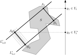
Figure 6. An illustration for the proof of Lemma 2.10. The element $y_{1}$ of $Y_{t}$ is half-isolated while $y_{2}$ is not.

Choose $y\in Y_{t}^{*}$, and define $(A_{y},B_{y})\colonequals\tau(a,b,c,y)$. We claim that $\overline{A_{y}B_{y}}\cap{S}^{\circ}$ is either empty or a single interval. Let us choose any two points $C,D\in\overline{A_{y}B_{y}}\cap{S}^{\circ}$. We will show that the segment $\overline{CD}$ is inside ${S}^{\circ}$. For $\varepsilon>0$ small enough, the neighborhoods $\mathcal{N}_{\varepsilon}(C)$ and $\mathcal{N}_{\varepsilon}(D)$ are subsets of $S$. Since $y$ is not half-isolated in $Y_{t}$, we can find two segments $P,Q\in\mathfrak{B}_{\bullet}$ of type $t$ that intersect both $\mathcal{N}_{\varepsilon}(C)$ and $\mathcal{N}_{\varepsilon}(D)$, with $\overline{A_{y}B_{y}}$ being between $P$ and $Q$. We can then find a closed polygonal curve $\Gamma\subseteq P\cup Q\cup\mathcal{N}_{\varepsilon}(C)\cup\mathcal{N}_{\varepsilon}(D)$ whose interior region contains $\overline{CD}$. Since $S$ is p-componentwise simply connected, we see that $\overline{CD}\subseteq{S}^{\circ}$. Therefore, $\overline{A_{y}B_{y}}\cap{S}^{\circ}$ is indeed an interval.

Since $\partial S$ is a closed set, we know that for every $y\in Y_{t}^{*}$, the set $\overline{A_{y}B_{y}}\cap\partial S$ is closed as well. Moreover, neither $A_{y}$ nor $B_{y}$ are isolated boundary points of $\overline{A_{y}B_{y}}$, because then $(A_{y},B_{y})$ would belong to $\mathfrak{B}_{\lhd}$ or $\mathfrak{B}_{\rhd}$. We conclude that $\overline{A_{y}B_{y}}\cap\partial S$ is either equal to a single closed segment of positive length containing $A_{y}$ or $B_{y}$, or it is equal to a disjoint union of two closed segments of positive length, one of which contains $A_{y}$ and the other contains $B_{y}$.

For an integer $n\in\mathbb{N}$, define two sets $Y_{t}^{\lhd}(n)$ and $Y_{t}^{\rhd}(n)$ by

$$Y_{t}^{\lhd}(n) \colonequals\{y\in Y_{t}^{*}\colon\overline{A_{y}B_{y}}[(0,n^{-1})]\subseteq\partial S\},$$

$$Y_{t}^{\rhd}(n) \colonequals\{y\in Y_{t}^{*}\colon\overline{A_{y}B_{y}}[(1-n^{-1},1)]\subseteq\partial S\}.$$

Note that these sets are measurable: for instance, $Y_{t}^{\lhd}(n)$ is equal to $Y_{t}^{*}\smallsetminus\left(\bigcup_{\alpha}Y_{t}(\alpha)\right)$, where we take the union over all rational intervals $\alpha$ intersecting $(0,n^{-1})$. Moreover, we have $Y_{t}^{*}=\bigcup_{n\in\mathbb{N}}(Y_{t}^{\lhd}(n)\cup Y_{t}^{\rhd}(n))$. It follows that there is an $n$ such that $Y_{t}^{\lhd}(n)$ or $Y_{t}^{\rhd}(n)$ has positive measure. Fix such an $n$ and assume, without loss of generality, that $\lambda_{1}(Y_{t}^{\lhd}(n))$ is positive. Define the region of $t$, denoted by $R_{t}$, by

$$R_{t}\colonequals\bigcup_{y\in Y_{t}^{\lhd}(n)}\overline{A_{y}B_{y}}[(0,n^{-1})].$$

The set $R_{t}$ is a bijective affine image of $Y_{t}^{\lhd}(n)\times(0,n^{-1})$, and in particular it is $\lambda_{2}$-measurable with positive measure. Note that $R_{t}$ is a subset of $\partial S$.

Consider now two types $t,t^{\prime}\in\mathbb{R}^{3}\smallsetminus T_{0}$ with distinct slopes, such that both $Y_{t}$ and $Y_{t^{\prime}}$ have positive measure. We will show that the regions $R_{t}$ and $R_{t^{\prime}}$ are disjoint.

For contradiction, suppose there is a point $C\in R_{t}\cap R_{t^{\prime}}$. Let $\overline{AB}$ and $\overline{A^{\prime}B^{\prime}}$ be the segments containing $C$ and having types $t$ and $t^{\prime}$, respectively. Fix $\varepsilon>0$ small enough, so that none of the four endpoints $A,B,A^{\prime},B^{\prime}$ lies in $\mathcal{N}_{\varepsilon}(C)$. Since $Y_{t}^{*}$ has no half-isolated points of $Y_{t}$, we know that $\mathfrak{B}_{\bullet}$ has segments of type $t$ arbitrarily close to $\overline{AB}$ on both sides of $\overline{AB}$, and similarly for segments of type $t^{\prime}$ close to $\overline{A^{\prime}B^{\prime}}$. We can therefore find four segments $P,Q,P^{\prime},Q^{\prime}\in\mathfrak{B}_{\bullet}\smallsetminus\{\overline{AB},\overline{A^{\prime}B^{\prime}}\}$ with these properties:

• $P$ and $Q$ have type $t$, and $P^{\prime}$ and $Q^{\prime}$ have type $t^{\prime}$.

• $\overline{AB}$ is between $P$ and $Q$ (i.e., $\overline{AB}\subseteq\operatorname{Conv}(P\cup Q)$) and $\overline{A^{\prime}B^{\prime}}$ is between $P^{\prime}$ and $Q^{\prime}$.

• Both $P$ and $Q$ intersect both $P^{\prime}$ and $Q^{\prime}$ inside $\mathcal{N}_{\varepsilon}(C)$.

We see that the four points where $P\cup Q$ intersects $P^{\prime}\cup Q^{\prime}$ form the vertex set of a parallelogram $W$ whose interior contains the point $C$. Moreover, the boundary of $W$ is a closed polygonal curve contained in $S$. Since $S$ is p-componentwise simply connected, $W$ is a subset of $S$ and $C$ belongs to ${S}^{\circ}$. This is a contradiction, since all points of $R_{t}$ (and $R_{t^{\prime}}$) belong to $\partial S$.

We conclude that $R_{t}$ and $R_{t^{\prime}}$ are indeed disjoint. Since there cannot be uncountably many disjoint sets of positive measure in $\mathbb{R}^{2}$, there are at most countably many values $a\in\mathbb{R}$ for which there is a type $t=(a,b,c)$ with $\lambda_{1}(Y_{t})$ positive. Consequently, the right-hand side of ($*$ ‣ 2.2) is zero, and so $\lambda_{4}(\mathfrak{B}_{\bullet})=0$, as claimed. ∎

Proof of Lemma 2.1.

Observe that the inequalities $\operatorname{b}(S)\leqslant\alpha\operatorname{c}(S)$ and $\lambda_{4}(\operatorname{Seg}(S))\leqslant\alpha\operatorname{smc}(S)\cdot\lambda_{2}(S)$ are equivalent. Call a set $S$ bad if $\operatorname{Seg}(S)$ is measurable and $\operatorname{b}(S)>\alpha\operatorname{c}(S)$ or equivalently $\lambda_{4}(\operatorname{Seg}(S))>\alpha\operatorname{smc}(S)\lambda_{2}(S)$. To prove the lemma, we suppose for the sake of contradiction that there exists a bad p-componentwise simply connected set $S\subseteq\mathbb{R}^{2}$ of finite positive measure.

By Lemma 2.9, for each $\varepsilon>0$, there is a bounded p-componentwise simply connected set $S^{\prime}\subseteq S$ such that $\lambda_{2}(S^{\prime})\geqslant(1-\varepsilon)\lambda_{2}(S)$ and $\operatorname{b}(S^{\prime})\geqslant\operatorname{b}(S)-\varepsilon$. In particular, such a set $S^{\prime}$ satisfies $\operatorname{c}(S^{\prime})\leqslant\operatorname{c}(S)/(1-\varepsilon)$. Hence, for $\varepsilon$ small enough, the set $S^{\prime}$ is bad.

Let $S^{\prime\prime}$ be the interior of $S^{\prime}$. By Lemma 2.10, $\lambda_{4}(\operatorname{Seg}(S^{\prime\prime}))=\lambda_{4}(\operatorname{Seg}(S^{\prime}))$. Clearly, $\lambda_{2}(S^{\prime\prime})\leqslant\lambda_{2}(S^{\prime})$ and $\operatorname{smc}(S^{\prime\prime})\leqslant\operatorname{smc}(S^{\prime})$, and therefore $S^{\prime\prime}$ is bad as well.

Note that $S^{\prime\prime}$ is p-componentwise simply connected. Since $S^{\prime\prime}$ is an open set, all its p-components are open as well. In particular, $S^{\prime\prime}$ has at most countably many p-components. Let $\mathcal{C}$ be the set of p-components of $S^{\prime\prime}$. Each $T\in\mathcal{C}$ is a bounded open simply connected set, and therefore cannot be bad. Therefore,

$$\lambda_{4}(\operatorname{Seg}(S^{\prime\prime}))=\sum_{T\in\mathcal{C}}\lambda_{4}(\operatorname{Seg}(T))\leqslant\sum_{T\in\mathcal{C}}\alpha\operatorname{smc}(T)\lambda_{2}(T)\leqslant\alpha\operatorname{smc}(S^{\prime\prime})\lambda_{2}(S^{\prime\prime}),$$

showing that $S^{\prime\prime}$ is not bad. This is a contradiction. ∎

2.3. Proof of Lemma 2.4

Here we prove Lemma 2.4, which says that every bounded open simply connected subset of $\mathbb{R}^{2}$ can can be split by a diagonal into two rooted sets.

Lemma 2.11.

Let $S$ be a bounded open simply connected subset of $\mathbb{R}^{2}$, and let $\ell$ be a diagonal of $S$. Let $h^{-}$ and $h^{+}$ be the open half-planes defined by the supporting line of $\ell$. It follows that the set $S\smallsetminus\ell$ has exactly two p-components $S_{1}$ and $S_{2}$. Moreover, for every point $A\in\ell$ and every neighborhood $\mathcal{N}_{\varepsilon}(A)\subseteq S$, we have $\mathcal{N}_{\varepsilon}(A)\cap h^{-}\subseteq S_{1}$ and $\mathcal{N}_{\varepsilon}(A)\cap h^{+}\subseteq S_{2}$.

Proof.

Notice first that any p-component of an open set is also open. This implies that any path-connected open set is also p-connected, and therefore every open simply connected set is p-connected as well.

Let $A\in\ell$, and let $\mathcal{N}_{\varepsilon}(A)$ be a neighborhood of $A$ contained in $S$. We choose arbitrary points $B\in\mathcal{N}_{\varepsilon}(A)\cap h^{-}$ and $C\in\mathcal{N}_{\varepsilon}(A)\cap h^{+}$. Suppose for a contradiction that $S\smallsetminus\ell$ has a single p-component. Then there exists a polygonal curve $\Gamma$ in $S\smallsetminus\ell$ with endpoints $B$ and $C$. Let $\Delta\subseteq S$ be the closed polygonal curve $\Gamma\cup\overline{BC}$. We can assume that the curve $\Delta$ is simple using a local redrawing argument. See Figure 7.

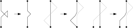
Figure 7. Removing self-intersections and intersections between adjacent polygonal lines.

The curve $\Delta$ separates $\mathbb{R}^{2}$ into two regions. The closure $\overline{\ell}$ of the diagonal $\ell$ is a closed line segment that intersects $\Delta$ in exactly one point. It follows that one endpoint of $\ell$ is in the interior region of $\Delta$. Since the endpoints of $\ell$ do not belong to $S$, this contradicts the assumption that $S$ is simply connected.

Now, we show that the set $S\smallsetminus\ell$ has at most two p-components. For a point $D\in\ell$, let $\mathcal{N}_{\varepsilon}(D)$ be a neighborhood of $D$ in $S$. The set $\mathcal{N}_{\varepsilon}(D)\cap h^{-}$ is contained in a unique p-component $S_{1}$ of $S\smallsetminus\ell$, and $\mathcal{N}_{\varepsilon}(D)\cap h^{+}$ is contained in a different p-component $S_{2}$. Choose another point $E\in\ell$ with a neighborhood $\mathcal{N}_{\varepsilon^{\prime}}(E)\subseteq S$. We claim that $\mathcal{N}_{\varepsilon^{\prime}}(E)\cap h^{-}$ also belongs to $S_{1}$. To see this, note that since $\overline{DE}$ is a compact subset of the open set $S$, it has a neighborhood $\mathcal{N}_{\delta}(\overline{DE})$ which is contained in $S$. Clearly, $\mathcal{N}_{\delta}(\overline{DE})\cap h^{-}$ is p-connected and therefore belongs to $S_{1}$, hence $\mathcal{N}_{\varepsilon^{\prime}}(E)\cap h^{-}$ belongs to $S_{1}$ as well. An analogous argument can be made for the half-plane $h^{+}$ and the p-component $S_{2}$.

Since for every p-component $S^{\prime}$ of $S\smallsetminus\ell$, there is a point $A\in\ell$ and a neighborhood $\mathcal{N}_{\varepsilon}(A)\subseteq S$ such that $\mathcal{N}_{\varepsilon}(A)\cap S^{\prime}\neq\emptyset$, we see that $S_{1}$ and $S_{2}$ are the only two p-components of $S\smallsetminus\ell$. ∎

Proof of Lemma 2.4.

By Lemma 2.11, the set $S\smallsetminus\ell$ has of exactly two p-components $S_{1}$ and $S_{2}$. It remains to show that $S_{1}\cup\ell$ and $S_{2}\cup\ell$ are rooted sets.

Since $S_{1}$ and $S_{2}$ are p-connected, $S_{1}\cup\ell$ and $S_{2}\cup\ell$ are p-connected as well. To show that $S_{1}\cup\ell$ and $S_{2}\cup\ell$ are simply connected, choose a Jordan curve $\Gamma$ in, say, $S_{1}\cup\ell$, and let $Z$ be the interior region of $\Gamma$. Suppose for a contradiction that $Z$ is not a subset of $S_{1}\cup\ell$. Since $S$ is simply connected, we have $Z\subseteq S$. Hence there is a point $A\in Z\cap S_{2}$. Since both $S_{2}$ and $Z$ are open, we can assume that $A$ does not lie on the supporting line of $\ell$. Let $\overline{AB}$ be the minimal closed segment parallel to $\ell$ such that $B\in\Gamma$. Then $B$ belongs to $S_{1}$, $A$ belongs to $S_{2}$, and yet $A$ and $B$ are in the same p-component of $S\smallsetminus\ell$. This contradiction shows that $S_{1}\cup\ell$ and $S_{2}\cup\ell$ are simply connected.

As subsets of the bounded set $S$, the sets $S_{1}\cup\ell$ and $S_{2}\cup\ell$ are bounded. Lemma 2.11 and the fact that $S_{i}$ is open imply that the set $S_{i}\cup\ell$ is half-open and $S_{i}\cap\partial S_{i}=\ell$ for $i\in\{1,2\}$. Therefore, the sets $S_{1}\cup\ell$ and $S_{2}\cup\ell$ are rooted, and $\ell$ is their root. ∎

2.4. Proof of Lemma 2.5

Here we prove Lemma 2.5, which explains the tree structure of rooted sets. For this entire section, let $R$ be a rooted set and $(L_{k})_{k\geqslant 1}$ be the partition of $R$ into levels. We will need several auxiliary results in order to prove Lemma 2.5.

For disjoint sets $S,T\subseteq\mathbb{R}^{2}$, we say that the set $S$ is $T$-half-open if every point $A\in S$ has a neighborhood $\mathcal{N}_{\varepsilon}(A)$ that satisfies one of the following two conditions:

1. $\mathcal{N}_{\varepsilon}(A)\subseteq S$,

2. $\mathcal{N}_{\varepsilon}(A)\cap\partial S$ is a diameter of $\mathcal{N}_{\varepsilon}(A)$ splitting it into two subsets, one of which (including the diameter) is $\mathcal{N}_{\varepsilon}(A)\cap S$ and the other (excluding the diameter) is $\mathcal{N}_{\varepsilon}(A)\cap T$.

The only difference with the definition of $S$ being half-open is that we additionally specify the “other side” of the neighborhoods $\mathcal{N}_{\varepsilon}(A)$ for points $A\in S\cap\partial S$ in the condition 2. A rooted set $R$ is $T$-half-open if and only if it is attached to $T$ according to the definition of attachment from Section 2.

Lemma 2.12.

The set $L_{1}$ is $(\mathbb{R}^{2}\smallsetminus R)$-half-open and $L_{1}\cap\partial L_{1}=R\cap\partial R$.

Proof.

We consider two cases for a point $A\in L_{1}$. First, suppose $A\in L_{1}\cap\partial R$. It follows that $A$ has a neighborhood $\mathcal{N}_{\varepsilon}(A)$ that satisfies the condition 2 of the definition of a half-open set. By the definition of $L_{1}$, the same neighborhood $\mathcal{N}_{\varepsilon}(A)$ satisfies the condition 2 for $L_{1}$ being an $(\mathbb{R}^{2}\smallsetminus R)$-half-open set. In particular, $A\in\partial L_{1}$. Since $R\cap\partial R\subseteq L_{1}$ by the definition of $L_{1}$, we have $R\cap\partial R\subseteq L_{1}\cap\partial L_{1}$.

Now, suppose $A\in L_{1}\cap{R}^{\circ}$. Let $B$ be a point of the root of $R$ such that $\overline{AB}\subseteq R$. We have $\overline{AB}\smallsetminus\{B\}\subseteq{R}^{\circ}$, as otherwise the point $t^{\prime}A+(1-t^{\prime})B$ for $t^{\prime}\colonequals\sup\{t\in[0,1]\colon At+(1-t)B\in\overline{AB}\cap\partial R\}$ would contradict the fact that $R$ is half-open. There is a family of neighborhoods $\{\mathcal{N}_{\varepsilon_{C}}(C)\}_{C\in\overline{AB}}$ such that all $\mathcal{N}_{\varepsilon_{D}}(D)$ with $D\in\overline{AB}\smallsetminus\{B\}$ satisfy the condition 1 and $\mathcal{N}_{\varepsilon_{B}}(B)$ satisfies the condition 2 for $R$ being half-open. Since $\overline{AB}$ is compact, there is a finite set $X\subseteq\overline{AB}$ such that $\overline{AB}\subseteq\bigcup_{C\in X}\mathcal{N}_{\varepsilon_{C}/2}(C)$. Hence $\mathcal{N}_{\varepsilon}(\overline{AB})\subseteq\bigcup_{C\in X}\mathcal{N}_{\varepsilon_{C}}(C)$, where $\varepsilon\colonequals\min_{C\in X}\varepsilon_{C}/2$. It follows that $\mathcal{N}_{\varepsilon}(\overline{AB})\cap\partial R$ is an open segment $Q$ containing $B$ but not $A$ and splitting $\mathcal{N}_{\varepsilon}(\overline{AB})$ into two subsets, one of which (including $Q$) is $\mathcal{N}_{\varepsilon}(\overline{AB})\cap R$ and the other (excluding $Q$) is $\mathcal{N}_{\varepsilon}(\overline{AB})\smallsetminus R$. Let $\varepsilon^{\prime}$ be the minimum of $\varepsilon$ and the distance of $A$ to the line containing $Q$. It follows that $\mathcal{N}_{\varepsilon^{\prime}}(A)\subseteq\mathcal{N}_{\varepsilon}(\overline{AB})\cap R$. Therefore, for every $A^{\prime}\in\mathcal{N}_{\varepsilon^{\prime}}(A)$, we have $\overline{A^{\prime}B}\subseteq R$, hence $\mathcal{N}_{\varepsilon^{\prime}}(A)\subseteq L_{1}$. It also follows that $L_{1}\cap\partial L_{1}\subseteq R\cap\partial R$. ∎

We say that a set $P\subseteq R$ is $R$-convex when the following holds for any two points $A,B\in P$: if $\overline{AB}\subseteq R$, then $\overline{AB}\subseteq P$.

Lemma 2.13.

The set $L_{1}$ is $R$-convex.

Proof.

This follows directly from Lemma 2.3. ∎

A branch of $R$ is a p-component of $\bigcup_{k\geqslant 2}L_{k}$.

Lemma 2.14.

Every branch of $R$ is $R$-convex.

Proof.

Let $P$ be a branch of $R$, and let $A,B\in P$ be such that $\overline{AB}\subseteq R$. Since $R$ is half-open, it follows that $\overline{AB}\subseteq{R}^{\circ}$. Suppose $\overline{AB}\not\subseteq P$. It follows that $\overline{AB}\cap L_{1}\neq\emptyset$. Since $L_{1}$ is $(\mathbb{R}^{2}\smallsetminus R)$-half-open (Lemma 2.12) and $R$-convex (Lemma 2.13), we see that $\overline{AB}\cap L_{1}$ is an open segment $A^{\prime}B^{\prime}$ for some $A^{\prime},B^{\prime}\in\overline{AB}$. It follows that $A^{\prime},B^{\prime}\in P$.

There is a simple polygonal line in $P$ connecting $A^{\prime}$ with $B^{\prime}$, which together with $\overline{A^{\prime}B^{\prime}}$ forms a Jordan curve $\Gamma$ in $R$. Now, let $C\in A^{\prime}B^{\prime}$. Since $C\in L_{1}$, there is a point $D$ on the root of $R$ such that $\overline{CD}\subseteq R$. Since $A^{\prime},B^{\prime}\notin L_{1}$, $D$ does not lie on the supporting line of $A^{\prime}B^{\prime}$. Extend the segment $DC$ beyond $C$ until hitting $\partial R$ at a point $C^{\prime}$. Here we use the fact that $R$ is bounded. Since $R$ is simply connected, the entire interior region of $\Gamma$ is contained in $R$, so the points $D$ and $C^{\prime}$ both lie in the exterior region of $\Gamma$. However, since $\Gamma\cap L_{1}=A^{\prime}B^{\prime}$, the line segment $\overline{DC^{\prime}}$ crosses $\Gamma$ at exactly one point, which is $C$. This is a contradiction. ∎

Lemma 2.15.

The set $L_{1}$ and every branch of $R$ are p-connected and simply connected.

Proof.

Let $P$ be the set $L_{1}$ or a branch of $R$. It follows directly from the definitions of $L_{1}$ and a branch of $R$ that $P$ is p-connected. To see that $P$ is simply connected, let $\Gamma$ be a Jordan curve in $P$, $A$ be a point in the interior region of $\Gamma$, and $BC$ be an inclusion-maximal open line segment in the interior region of $\Gamma$ such that $A\in BC$. It follows that $B,C\in\Gamma$ and $\overline{BC}\subseteq R$, as $R$ is simply connected. Since $B,C\in P$ and $P$ is $R$-convex (Lemmas 2.13 and 2.14), we have $A\in P$. ∎

Lemma 2.16.

Every branch of $R$ is $L_{1}$-half-open.

Proof.

Let $P$ be a branch of $R$. It is enough to check the condition 2 for $P$ being $L_{1}$-half-open for points in $\partial P\cap P$. Let $A\in\partial P\cap P$. Since $R$ is half-open, $A$ has a neighborhood $\mathcal{N}_{\varepsilon}(A)$ that satisfies the condition 1 or 2 for $S$ being half-open. It cannot be 2, as then $A$ would lie on the root of $R$ and thus in $L_{1}$. Hence $\mathcal{N}_{\varepsilon}(A)\subseteq R$.

Since $L_{1}$ is $(\mathbb{R}^{2}\smallsetminus R)$-half-open (Lemma 2.12) and $R$-convex (Lemma 2.13) and $A\notin L_{1}$, the set $\mathcal{N}_{\varepsilon}(A)\cap L_{1}$ lies entirely in some open half-plane $h$ whose boundary line passes through $A$. The set $\mathcal{N}_{\varepsilon}(A)\smallsetminus h$ is p-connected and contains $A$, so it lies entirely within $P$. The set $\mathcal{N}_{\varepsilon}(A)\cap h$ is disjoint from $P$. Indeed, if there was a point $B\in\mathcal{N}_{\varepsilon}(A)\cap h\cap P$, then by the $R$-convexity of $P$ (Lemma 2.14), the convex hull of $\mathcal{N}_{\varepsilon}(A)\smallsetminus h$ and $B$ would lie entirely within $P$ and would contain $A$ in its interior, which would contradict the assumption that $A\in\partial P$. It follows that $\mathcal{N}_{\varepsilon}(A)\cap\partial P$ is an open segment that partitions $\mathcal{N}_{\varepsilon}(A)$ into two half-discs, one of which (including $\mathcal{N}_{\varepsilon}(A)\cap\partial P$) is $\mathcal{N}_{\varepsilon}(A)\cap P$.

We show that $\mathcal{N}_{\varepsilon}(A)\cap\partial P\subseteq\partial L_{1}$. Suppose to the contrary that there is a point $A^{\prime}\in\mathcal{N}_{\varepsilon}(A)\cap\partial P\smallsetminus\overline{L_{1}}$. It follows that $A^{\prime}$ has a neighborhood $\mathcal{N}_{\varepsilon^{\prime}}(A^{\prime})\subseteq\mathcal{N}_{\varepsilon}(A)\smallsetminus\overline{L_{1}}$. Since $\mathcal{N}_{\varepsilon^{\prime}}(A^{\prime})$ is p-connected and contains a point of $P$, it lies entirely within $P$. This contradicts the assumption that $A^{\prime}\in\partial P$.

Since $\mathcal{N}_{\varepsilon}(A)\cap\partial P\subseteq\partial L_{1}$, there is a point $B\in\mathcal{N}_{\varepsilon}(A)\cap L_{1}$. Let $A^{\prime}\in\mathcal{N}_{\varepsilon}(A)\cap\partial P$. Since $L_{1}$ is $(\mathbb{R}^{2}\smallsetminus R)$-half-open and $R$-convex and $A\notin L_{1}$, there is a point $C\in\overline{A^{\prime}B}$ such that $\overline{CB}\smallsetminus\{C\}\subseteq L_{1}$ while $\overline{A^{\prime}C}$ is disjoint from $L_{1}$. The latter implies that $\overline{A^{\prime}C}\subseteq P$, as $A^{\prime}\in P$. Hence $C=A^{\prime}$. This shows the whole triangle $T$ spanned by $\mathcal{N}_{\varepsilon}(A)\cap\partial P$ and $B$ excluding the open segment $\mathcal{N}_{\varepsilon}(A)\cap\partial P$ is contained in $L_{1}$.

Since $A$ lies in the interior of $\mathcal{N}_{\varepsilon}(A)\cap(P\cup T)$, it has a neighborhood $\mathcal{N}_{\varepsilon^{\prime}}(A)$ that lies entirely within $\mathcal{N}_{\varepsilon}(A)\cap(P\cup T)$. This neighborhood witnesses the condition 2 for $P$ being $L_{1}$-half-open. ∎

Lemma 2.17.

Let $P$ be a branch of $R$. If $A_{0},A_{1}\in P\cap\partial P$, then $\overline{A_{0}A_{1}}\subseteq R$.

Proof.

Let $A_{0},A_{1}\in P\cap\partial P$. By Lemma 2.16, $P$ is $L_{1}$-half-open, hence there are $B_{0},B_{1}\in L_{1}$ such that $\overline{A_{0}B_{0}}\smallsetminus\{A_{0}\}\subseteq L_{1}$ and $\overline{A_{1}B_{1}}\smallsetminus\{A_{1}\}\subseteq L_{1}$. There is a polygonal line $\Gamma_{1}$ in $P$ connecting $A_{0}$ with $A_{1}$, and a polygonal line $\Gamma_{2}$ in $L_{1}$ connecting $B_{0}$ with $B_{1}$. These polygonal lines together with the line segments $\overline{A_{0}B_{0}}$ and $\overline{A_{1}B_{1}}$ form a closed polygonal curve $\Gamma$ in $R$. We can assume without loss of generality that $\Gamma$ is simple (see Figure 7) and that the $x$-coordinates of $A_{0}$ and $A_{1}$ are equal to $0$. We also assume that no two vertices of $\Gamma$ except $A_{0}$ and $A_{1}$ have the same $x$-coordinates.

We color the points of $\Gamma\cap L_{1}$ red and the points of $\Gamma\cap P$ blue. For convenience, we assume that $A_{0}$ and $A_{1}$ have both colors. Let $Z$ denote the interior region delimited by $\Gamma$ including $\Gamma$ itself. Since $R$ is simply connected, we have $Z\subseteq R$.

Let $x_{1}<\dotsb<x_{n}$ be the $x$-coordinates of all vertices of $\Gamma$. We use $[n]$ to denote the set of indices $\{1,\dotsc,n\}$. Since the $x$-coordinates of $A_{0}$ and $A_{1}$ are zero, there is $j\in[n]$ such that $x_{j}=0$. For $i\in[n]$, we let $l_{i}$ be the vertical line $\{x_{i}\}\times\mathbb{R}$. Since the $x$-coordinates of the vertices of $\Gamma\smallsetminus\{A_{0},A_{1}\}$ are distinct, there is at most one vertex of $\Gamma$ on $l_{i}$ for every $i\in[n]\smallsetminus\{j\}$. For $i\in[n]$, the intersection of $Z$ with $l_{i}$ is a family of closed line segments with endpoints from $\Gamma\cap l_{i}$. Some of the segments can be trivial, that is, consisting of a single point, and some segments can contain a point of $\Gamma$ in their interior.

For $i\in[n]$ and a point $A\in\Gamma\cap l_{i}$, we say that a point $B$ is a left neighbor of $A$ if $B$ lies on $\Gamma\cap l_{i-1}$ and $\overline{AB}\subseteq\Gamma$. Similarly, $B$ is a right neighbor of $A$ if $B\in\Gamma\cap l_{i+1}$ and $\overline{AB}\subseteq\Gamma$. Note that every point $A\in\Gamma\cap l_{i}$ has exactly two neighbors and if $A\notin\{A_{0},A_{1}\}$, then the neighbors of $A$ have the same color as $A$. We distinguish two types of points of $\Gamma\cap l_{i}$. We say that a point $A\in\Gamma\cap l_{i}$ is one-sided if it either has two right or two left neighbors. Otherwise, we say that $A$ is two-sided. That is, $A$ is two-sided if it has one left and one right neighbor. See Figure 8.

Note that every one-sided point is a vertex of $\Gamma$ and that one-sided points from $\Gamma\cap l_{i}$ are exactly the points of $\Gamma\cap l_{i}$ that either form a trivial line segment or that are contained in the interior of some line segment of $Z\cap l_{i}$. Consequently, every line segment in $Z\cap l_{i}$ contains at most one point of $\Gamma$ in its interior.

For $2\leqslant i\leqslant n$ and $C,D\in l_{i}\cap\Gamma$, let $\overline{CD}$ be a line segment in $Z\cap l_{i}$ whose interior does not contain a point of $\Gamma$ with a left neighbor. Let $A$ and $B$ be left neighbors of $C$ and $D$, respectively, such that there is no left neighbor of $C$ and $D$ between $A$ and $B$ on $l_{i-1}$. Since no point between $A$ and $B$ on $l_{i-1}$ can have a right neighbor, we have $\overline{AB}\subseteq Z\cap l_{i-1}$ and $A,B,C,D$ are vertices of a trapezoid whose interior is contained in $Z$. An analogous statement holds for right neighbors of $C$ and $D$ provided that the interior of $\overline{CD}$ does not contain a point of $\Gamma$ with a right neighbor.

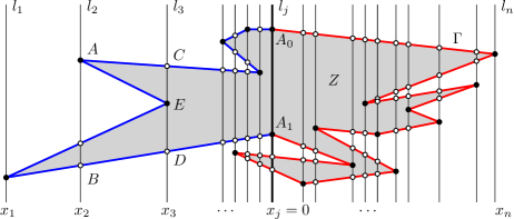
Figure 8. Situation in the proof of Lemma 2.17. Here $A$ is a left neighbor of $C$ and $B$ is a left neighbor of $D$. The points $B$, $C$, and $D$ are two-sided, the points $A$ and $E$ are one-sided.

Claim.

Let $i\in[n]\smallsetminus\{j\}$, and let $C$ and $D$ be points of $\Gamma\cap l_{i}$ satisfying $\overline{CD}\subseteq Z\cap l_{i}$. Then $C$ and $D$ have the same color.

First, we will prove the claim by induction on $i$ for all $i<j$. The claim clearly holds for $i=1$, as $Z\cap l_{1}$ contains only a single vertex of $\Gamma$. Fix $i$ with $1<i<j$ and suppose that the claim holds for $i-1$. Let $C,D\in\Gamma\cap l_{i}$ be points satisfying $\overline{CD}\subseteq Z\cap l_{i}$. We show that $C$ and $D$ have the same color. Obviously, we can assume that the line segment $\overline{CD}$ is non-trivial. Assume first that the points $C$ and $D$ are two-sided.

Suppose the interior of $\overline{CD}$ does not contain a point of $\Gamma$ with a left neighbor. Let $A,B\in\Gamma\cap l_{i-1}$ be the left neighbors of $C$ and $D$, respectively. Then $\overline{AB}\subseteq Z\cap l_{i-1}$. Thus $A$ and $B$ have the same color by the induction hypothesis. Since $C,D\notin\{A_{0},A_{1}\}$, the points $A$ and $C$ have the same color as well as the points $B$ and $D$. This implies that $C$ and $D$ have the same color too. If there is a point $E$ of $\Gamma$ in the interior of $\overline{CD}$, then it follows from $R$-convexity of $P$ (Lemma 2.14) and $L_{1}$ (Lemma 2.13) that $E$ has the same color as $C$ and $D$.

Now, suppose the interior of $\overline{CD}$ contains a point $E$ of $\Gamma$ with a left neighbor. We have already observed that there is exactly one such point on $\overline{CD}$. We also know that $E$ has two left neighbors. The points $C$ and $E$ with their left neighbors $A$ and $B$, respectively, where there is no left neighbor of $E$ between $A$ and $B$ on $l_{i-1}$, form a trapezoid in $Z$ such that $\overline{AB}\subseteq Z\cap l_{i-1}$. From induction hypothesis $A$ and $B$ have the same color which implies that $C$ and $E$ have the same color as well. Similarly, $D$ and $E$ have the same color which implies that $C$ and $D$ have the same color as well.

The case where either $C$ or $D$ is one-sided is covered by the previous cases. The same inductive argument but in the reverse direction shows the claim for all $i$ with $j<i\leqslant n$. This completes the proof of the claim.

Now, consider the inclusion-maximal line segment $\overline{CD}$ of $Z\cap l_{j}$ that contains $A_{0}$. We can assume that either $C$ and $D$ are two-sided. Suppose for a contradiction that $A_{1}$ is not contained in $\overline{CD}$. If $\overline{CD}$ is trivial, that is, $C=D=A_{0}$, then $A_{0}$ is one-sided and its neighbors $A$ and $B$ have different colors, as $\Gamma$ changes color in $A_{0}$. This is impossible according to the claim, since we have $\overline{AB}\subseteq Z\cap l_{i-1}$ or $\overline{AB}\subseteq Z\cap l_{i+1}$. Therefore $\overline{CD}$ is non-trivial.

First, we assume that $A_{0}$ is an endpoint of $\overline{CD}$, say $C=A_{0}$. Then $A_{0}$ is two-sided. By symmetry, we can assume that the left neighbor $A$ of $A_{0}$ and the left neighbor $B$ of $D$ have different colors. If there is no point of $\Gamma$ with a left neighbor in the interior of $\overline{A_{0}D}$, then $\overline{AB}\subseteq Z\cap l_{i-1}$. This is impossible according to the claim. If there is a point $E\in\Gamma$ with a left neighbor in the interior of $\overline{A_{0}D}$, then we can use a similar argument either for the line segment $\overline{A_{0}E}$ or for $\overline{ED}$, as the neighbors of $E$ have the same color. The last case is when $A_{0}$ is an interior point of $\overline{CD}$. Since $\Gamma$ does not change color in $C$ nor in $D$, we apply the claim to one of the line segments $\overline{A_{0}C}$, $\overline{A_{0}D}$, and $\overline{CD}$ and show, again, that none of the cases is possible. Altogether, we have derived a contradiction.

Therefore, $A_{0}$ and $A_{1}$ are contained in the same line segment of $Z\cap l_{i}$. This completes the proof, as $Z\subseteq R$. ∎

Lemma 2.18.

For every branch $P$ of $R$, the set $P\cap\partial P$ is an open segment.

Proof.

Let $P$ be a branch of $R$. First, we show that the set $P\cap\partial P$ is convex. Let $A_{0},A_{1}\in P\cap\partial P$. By Lemma 2.17, we have $\overline{A_{0}A_{1}}\subseteq R$. It follows that $\overline{A_{0}A_{1}}$ is disjoint from the root of $R$ and thus is contained in ${R}^{\circ}$. By compactness, $\overline{A_{0}A_{1}}$ has a neighborhood $\mathcal{N}_{\varepsilon}(\overline{A_{0}A_{1}})$ contained in ${R}^{\circ}$. Since $P$ is $L_{1}$-half-open by Lemma 2.16, there are $B_{0},B_{1}\in\mathcal{N}_{\varepsilon}(\overline{A_{0}A_{1}})\cap L_{1}$ such that $\overline{A_{0}B_{0}}\smallsetminus\{A_{0}\}\subseteq L_{1}$ and $\overline{A_{1}B_{1}}\smallsetminus\{A_{1}\}\subseteq L_{1}$. For $t\in[0,1]$, let $A_{t}=(1-t)A_{0}+tA_{1}$ and $B_{t}=(1-t)B_{0}+tB_{1}$. We have $A_{t}\in\overline{A_{0}A_{1}}$ and $B_{t}\in\overline{B_{0}B_{1}}$, hence $A_{t},B_{t}\in\mathcal{N}_{\varepsilon}(\overline{A_{0}A_{1}})$, for all $t\in[0,1]$. Now, it follows from the $R$-convexity of $P$ (Lemma 2.14) and $L_{1}$ (Lemma 2.13) that $A_{t}\in P$ and $\overline{A_{t}B_{t}}\smallsetminus\{A_{t}\}\subseteq L_{1}$, hence $A_{t}\in P\cap\partial P$, for all $t\in[0,1]$. This shows that $P\cap\partial P$ is convex.

If $P\cap\partial P$ had three non-collinear points, then they would span a triangle with non-empty interior contained in $P\cap\partial P$, which would be a contradiction. Since $R$ is bounded, the set $P\cap\partial P$ is a line segment. That it is an open line segment follows directly from Lemma 2.16. ∎

Lemma 2.19.

For every $j\geqslant 2$, every p-component $P$ of $\bigcup_{k\geqslant j}L_{k}$ is a rooted set attached to $L_{j-1}$. Moreover, for $k\geqslant 1$, the $k$th level of $P$ is equal to $L_{j-1+k}\cap P$.

Proof.

The proof proceeds by induction on $j$. For the base case, let $P$ be a p-component of $\bigcup_{i\geqslant 2}L_{i}$, that is, a branch of $R$. It follows from Lemmas 2.15, 2.16 and 2.18 that $P$ is a rooted set attached to $L_{1}$. Let $\ell$ be the root of $P$, and let $(L^{\prime}_{k})_{k\geqslant 1}$ be the partition of $P$ into levels. We prove that $L^{\prime}_{k}\subseteq\bigcup_{i=1}^{k+1}L_{i}$ and $L_{k+1}\cap P\subseteq\bigcup_{i=1}^{k}L^{\prime}_{i}$ for every $k\geqslant 1$.

Let $A\in L^{\prime}_{k}$. It follows that there is a polygonal line $\Gamma$ with $k$ line segments connecting $A$ to a point $B\in\ell$. Moreover, since there is no shorter polygonal line connecting $A$ to $\ell$, the last line segment of $\Gamma$ is not parallel to $\ell$. Since $P$ is $L_{1}$-half-open (Lemma 2.16), there is a neighborhood $\mathcal{N}_{\varepsilon}(B)$ that is split by $\ell$ into two parts, one of which is a subset of $L_{1}$. Let $C$ be a point in $\mathcal{N}_{\varepsilon}(B)\cap L_{1}$ such that $\overline{BC}$ is an extension of the last line segment of $\Gamma$. Since $C\in L_{1}$, there is a point $D$ on the root of $R$ such that $\overline{CD}\subseteq L_{1}$. The polygonal line $\Gamma$ extended by $\overline{BC}$ and $\overline{CD}$ forms a polygonal line with $k+1$ line segments connecting $A$ to the root of $R$. This shows that $L^{\prime}_{k}\subseteq\bigcup_{i=1}^{k+1}L_{i}$.

Now, let $A\in L_{k+1}\cap P$. It follows that there is a polygonal line $\Gamma$ with $k+1$ line segments connecting $A$ to the root of $R$. Since $L_{1}$ is an open subset of $R$ (Lemma 2.12) and $P$ is a p-component of $R\smallsetminus L_{1}$, there is a point $B\in\Gamma$ such that the part of $\Gamma$ between $A$ and $B$ (inclusive) is contained in $P$ and is maximal with this property. It follows that $B\in\ell$. Since $B\notin L_{1}$, the part of $\Gamma$ between $A$ and $B$ consists of at most $k$ segments. This shows that $L_{k+1}\cap P\subseteq\bigcup_{i=1}^{k}L^{\prime}_{i}$.

We have thus proved that $L^{\prime}_{k}\subseteq\bigcup_{i=1}^{k+1}L_{i}$ and $L_{k+1}\cap P\subseteq\bigcup_{i=1}^{k}L^{\prime}_{i}$ for every $k\geqslant 1$. To conclude the proof of the base case, we note that a straightforward induction shows that $L^{\prime}_{k}=L_{k+1}\cap P$ for every $k\geqslant 1$.

For the induction step, let $j\geqslant 3$, and let $P$ be a p-component of $\bigcup_{i\geqslant j}L_{i}$. Let $Q$ be the branch of $R$ containing $P$. Let $(L^{\prime}_{k})_{k\geqslant 1}$ be the partition of $Q$ into levels. As we have proved for the base case, we have $L^{\prime}_{k}=L_{k+1}\cap Q$ for every $k\geqslant 1$. Hence $P$ is a p-component of $(\bigcup_{i\geqslant j}L_{i})\cap Q=\bigcup_{i\geqslant j-1}L^{\prime}_{i}$. By the induction hypothesis, $P$ is a rooted set attached to $L^{\prime}_{j-2}\subseteq L_{j-1}$. Moreover, for $k\geqslant 1$, the $k$th level of $P$ is equal to $L^{\prime}_{j-2+k}\cap P=L_{j-1+k}$. This completes the induction step and proves the lemma. ∎

Proof of Lemma 2.5.

The statement 1 is a direct consequence of the definition of a rooted set, specifically, of the condition that a rooted set is p-connected.

For the proof of the statement 2, let $P$ be a $j$-body of $R$. If $j=1$, then $P=L_{1}=\operatorname{Vis}(r,R)=\operatorname{Vis}(r,L_{1})$, where $r$ is the root of $R$, and by Lemmas 2.12 and 2.15, $L_{1}$ is rooted with the same root $r$. Now, suppose $j\geqslant 2$. Let $Q$ be the p-component of $\bigcup_{k\geqslant j}L_{k}$ containing $P$. By Lemma 2.19, $Q$ is a rooted set and $L_{j}\cap Q$ is the first level of $Q$. Since $P\subseteq L_{j}\cap Q$, the definition of the first level yields $P=L_{j}\cap Q=\operatorname{Vis}(r,Q)=\operatorname{Vis}(r,P)$, where $r$ is the root of $Q$. By Lemma 2.12, $P$ is a rooted set with the same root $r$.

Lemma 2.12 and the fact that $L_{1}$ is p-connected directly yield the statement 3.

Finally, for the proof of the statement 4, let $P$ be a $j$-body of $R$ with $j\geqslant 2$. Let $Q$ be the p-component of $\bigcup_{k\geqslant j}L_{k}$ containing $P$. As we have proved above, $Q$ is a rooted set and $P$ is the first level of $Q$ and shares the root with $Q$. Moreover, by Lemma 2.19, $Q$ (and hence $P$) is attached to $L_{j-1}$. The definition of attachment implies that $P$ is attached to a single p-component of $L_{j-1}$, that is, a single $(j-1)$-body of $R$. ∎

3. General dimension

This section is devoted to the proofs of Theorem 1.5 and Theorem 1.6. In both proofs, we use the operator $\operatorname{Aff}$ to denote the affine hull of a set of points.

3.1. Proof of Theorem 1.5

Let $T=(B_{0},B_{1},\dotsc,B_{d})$ be a $(d+1)$-tuple of distinct affinely independent points in $\mathbb{R}^{d}$. We say that a permutation $B_{0},B_{1},\dotsc,B_{d}$ of $T$ is a regular permutation of $T$ if the following two conditions hold:

1. the segment $\overline{B_{0}B_{1}}$ is the diameter of $T$,

2. for $i=2,\dotsc,d-1$, the point $B_{i}$ has the maximum distance to $\operatorname{Aff}(\{B_{0},\dotsc,B_{i-1}\})$ among the points $B_{i},B_{i+1},\dotsc,B_{d}$.

Obviously, $T$ has at least two regular permutations due to the interchangeability of $B_{0}$ and $B_{1}$. The regular permutation $B_{i_{0}},B_{i_{1}},\dotsc,B_{i_{d}}$ with the lexicographically minimal vector $({i_{0}},{i_{1}},\dotsc,{i_{d}})$ is called the canonical permutation of $T$.

Let $T$ be a $(d+1)$-tuple of distinct affinely independent points in $\mathbb{R}^{d}$, and let $B_{0},B_{1},\dotsc,B_{d}$ be the canonical permutation of $T$. For $i=1,\dotsc,d-1$, we define $\operatorname{Box}_{i}(T)$ inductively as follows:

1. $\operatorname{Box}_{1}(T)\colonequals\overline{B_{0}B_{1}}$,

2. for $i=2,\dotsc,d-1$, $\operatorname{Box}_{i}(T)$ is the box containing all the points $P\in\operatorname{Aff}(\{B_{0},B_{1},\dotsc,B_{i}\})$ with the following two properties:

   • the orthogonal projection of $P$ to $\operatorname{Aff}(\{B_{0},B_{1},\dotsc,B_{i-1}\})$ lies in $\operatorname{Box}_{i-1}(T)$,

   • the distance of $P$ to $\operatorname{Aff}(\{B_{0},B_{1},\dotsc,B_{i-1}\})$ does not exceed the distance of $B_{i}$ to $\operatorname{Aff}(\{B_{0},B_{1},\dotsc,B_{i-1}\})$,

3. $\operatorname{Box}_{d}(T)$ is the box containing all the points $P\in\mathbb{R}^{d}$ such that the orthogonal projection of $P$ to $\operatorname{Aff}(\{B_{0},B_{1},\dotsc,B_{d-1}\})$ lies in $\operatorname{Box}_{d-1}(T)$ and

   $$\lambda_{d}(\operatorname{Conv}(\{B_{0},B_{1},\dotsc,B_{d-1},P\}))\leqslant\lambda_{d}(S)\operatorname{c}(S).$$

The definition of $\operatorname{Box}_{d}(T)$ is independent of $B_{d}$, so we can define $\operatorname{Box}_{d}(T\smallsetminus\{B_{d}\})$ by

$$\operatorname{Box}_{d}(T\smallsetminus\{B_{d}\})\colonequals\operatorname{Box}_{d}(T).$$

It is not hard to see that this gives us a proper definition of $\operatorname{Box}_{d}(T^{-})$ for every $d$-tuple $T^{-}$ of $d$ distinct affinely independent points in $\mathbb{R}^{d}$.

Lemma 3.1.

1. For $i=1,\dotsc,d-1$, the box $\operatorname{Box}_{i}(T)$ contains the orthogonal projection of any point of $T$ to $\operatorname{Aff}(\{B_{0},B_{1},\dotsc,B_{i-1}\})$.

2. If $\operatorname{Conv}(T)\subseteq S$ then $\operatorname{Box}_{d}(T)$ contains the point $B_{d}$.

Proof.

We prove the statement 1 by induction on $i$. First, let $i=1$. Then the segment $\operatorname{Box}_{1}(T)$ must contain every point $A_{j}\in T$ since otherwise one of the segments $\overline{B_{0}A_{j}}$ and $\overline{B_{1}A_{j}}$ would be longer than the segment $\overline{B_{0}B_{1}}$. Further, if a point $A_{j}\in T$ satisfies the statement 1 for a parameter $i\in\{1,\dotsc,d-2\}$ then it also satisfies the statement 1 for the parameter $i+1$ since otherwise $A_{j}\neq B_{i+1}$ and $A_{j}$ should have been chosen for $B_{i+1}$.

The statement 2 follows from the fact that $\operatorname{Conv}(T)\subseteq S$ implies $\lambda_{d}(\operatorname{Conv}(T))\leqslant\operatorname{smc}(S)=\lambda_{d}(S)\operatorname{c}(S)$. ∎

For $i=1,\dotsc,d-1$, let $d_{i}$ be the distance of $B_{i}$ to $\operatorname{Aff}(\{B_{0},B_{1},\dotsc,B_{i-1}\})$. In particular, $d_{1}$ is the diameter of $T$. The following observation follows from the definition of the canonical permutation of $T$ and from the construction of the boxes $\operatorname{Box}_{i}(T)$.

Observation 3.2.

1. The $(d-1)$-dimensional measure of the simplex $\operatorname{Conv}(T\smallsetminus\{B_{d}\})$ is equal to $d_{1}d_{2}\dotsm d_{d-1}/(d-1)!$.

2. The sides of $\operatorname{Box}_{d}(T)$ have lengths $d_{1},2d_{2},\dotsc,2d_{d-1}$, and $\frac{d!}{d_{1}d_{2}\dotsm d_{d-1}}\lambda_{d}(S)\operatorname{c}(S)$.

Proof of Theorem 1.5.

To estimate $\operatorname{b}_{d}(S)$, we partition $\operatorname{Simp}_{d}(S)$ into the following $d+2$ subsets:

$$X \colonequals\{T\in\operatorname{Simp}_{d}(S)\colon\text{$T$ is affinely dependent}\},$$

$$Y_{i} \colonequals\{T=(A_{0},\dotsc,A_{d})\in\operatorname{Simp}_{d}(S)\colon\begin{minipage}[t]{210.0pt}\raggedright$T$ is affinely independent, and $A_{i}$ is the last\\ element of the canonical permutation of $T\}$,\\ for $i=0,\dotsc,d$.\@add@raggedright\end{minipage}$$

We point out that $T$ is considered to be affinely dependent in the above definitions of $X$ and $Y_{i}$ also in the degenerate case when some point of $S$ appears more than once in $T$. We have $\lambda_{d(d+1)}(X)=0$. Let $i\in\{0,\dotsc,d\}$. The set $Y_{i}$ is a subset of the set

$$Y_{i}^{\prime}\colonequals\{T=(A_{0},\dotsc,A_{d})\in S^{d+1}\colon\begin{minipage}[t]{210.0pt}\raggedright$T\smallsetminus\{A_{i}\}$ is affinely independent and we have\\ $A_{i}\in\operatorname{Box}_{d}(T\smallsetminus\{A_{i}\})\}$.\smash[t]{} \@add@raggedright\end{minipage}$$

By Observation 3.2 2, $\lambda_{d}(\operatorname{Box}_{d}(T\smallsetminus\{A_{i}\}))$ is equal to $z\colonequals 2^{d-2}d!\lambda_{d}(S)\operatorname{c}(S)$ for every set $T\smallsetminus\{A_{i}\}$ appearing in the definition of $Y_{i}^{\prime}$. Therefore, by Fubini’s Theorem, the set $Y_{i}^{\prime}$ is $\lambda_{d(d+1)}$-measurable and, moreover,

$$\lambda_{d(d+1)}(Y_{i}^{\prime})=(\lambda_{d}(S))^{d}z=(\lambda_{d}(S))^{d+1}2^{d-2}d!\operatorname{c}(S).$$

Thus,

$$\operatorname{b}_{d}(S)=\frac{\lambda_{d(d+1)}(\operatorname{Simp}_{d}(S))}{\lambda_{d}(S)^{d+1}}\leqslant\frac{\lambda_{d(d+1)}(X)+\sum_{i=0}^{d}\lambda_{d(d+1)}(Y_{i}^{\prime})}{\lambda_{d}(S)^{d+1}}=2^{d-2}(d+1)!\operatorname{c}(S).$$

This completes the proof of Theorem 1.5. ∎

3.2. Proof of Theorem 1.6

In the following, we make no serious effort to optimize the constants. As the first step towards the proof of Theorem 1.6, we show that if we remove an arbitrary $n$-tuple of points from the open $d$-dimensional box $(0,1)^{d}$, then the $d$-index of convexity of the resulting set is of order $\Omega(\frac{1}{n})$.

Lemma 3.3.

For every positive integer $n$ and every $n$-tuple $N$ of points from $(0,1)^{d}$, the set $S\colonequals(0,1)^{d}\smallsetminus N$ satisfies $\operatorname{b}_{d}(S)\geqslant 1/2n$.

Proof.

Let $S$ and $N=\{B_{1},\dotsc,B_{n}\}$ be the sets from the statement and let $0$ be the origin. We use $S^{d-1}_{*}$ to denote the set of $(d-1)$-tuples $(A_{1},\dotsc,A_{d-1})\in S^{d-1}$ that satisfy the following: for every $B\in N$ the points $A_{1},\dotsc,A_{d-1},B$ are affinely independent and $\operatorname{Aff}(\{A_{1},\dotsc,A_{d-1},B\})\cap(N\cup\{0\})=\{B\}$. Note that the set $S^{d-1}_{*}$ is measurable and $\lambda_{d(d-1)}(S^{d-1}_{*})=1$. If $h$ is a hyperplane in $\mathbb{R}^{d}$ that does not contain the origin, we use $h^{-}$ and $h^{+}$ to denote the open half-spaces defined by $h$ such that $0\in h^{-}$.

Let $(A_{1},\dotsc,A_{d-1})\in S^{d-1}_{*}$. For a point $B\in N$, we let $h_{A_{1},\dotsc,A_{d-1},B}$ be the hyperplane determined by the $d$-tuple $(A_{1},\dotsc,A_{d-1},B)$. Since $(A_{1},\dotsc,A_{d-1})\in S^{d-1}_{*}$, we see that $h_{A_{1},\dotsc,A_{d-1},B}$ satisfies $h_{A_{1},\dotsc,A_{d-1},B}\cap N=\{B\}$ and that it does not contain the origin. Therefore the half-spaces $\smash[t]{h_{A_{1},\dotsc,A_{d-1},B}^{-}}$ and $\smash[t]{h_{A_{1},\dotsc,A_{d-1},B}^{+}}$ are well defined.

For every $(d-1)$-tuple $(A_{1},\dotsc,A_{d-1})\in S^{d-1}_{*}$, we split the set $S$ into $2n$ pairwise disjoint open convex sets that are determined by the hyperplanes $h_{A_{1},\dotsc,A_{d-1},B}$ for $B\in N$. This is done by induction on $n$. For $n=1$, we set $P_{1}(A_{1},\dotsc,A_{d-1})\colonequals S\cap\smash[t]{h_{A_{1},\dotsc,A_{d-1},B_{1}}^{-}}$ and $P_{2}(A_{1},\dotsc,A_{d-1})\colonequals S\cap\smash[t]{h_{A_{1},\dotsc,A_{d-1},B_{1}}^{+}}$. Suppose we have split the set $S$ into sets $P_{i}(A_{1},\dotsc,A_{d-1})$ for $1\leqslant i\leqslant 2(n-1)$ and $n\geqslant 2$. Consider the hyperplane $h_{A_{1},\dotsc,A_{d-1},B_{n}}$. Since for every $k\in\{1,\dotsc,n-1\}$ the intersection $h_{A_{1},\dotsc,A_{d-1},B_{k}}\cap h_{A_{1},\dotsc,A_{d-1},B_{n}}$ is the affine hull of $A_{1},\dotsc,A_{d-1}$, we see that $h_{A_{1},\dotsc,A_{d-1},B_{n}}\smallsetminus\operatorname{Aff}(\{A_{1},\dotsc,A_{d-1}\})$ is contained in two sets $P_{i}(A_{1},\dotsc,A_{d-1})$ and $P_{j}(A_{1},\dotsc,A_{d-1})$ for some $1\leqslant i<j\leqslant 2(n-1)$. We restrict these sets to their intersection with the half-space $\smash[t]{h_{A_{1},\dotsc,A_{d-1},B_{n}}^{-}}$ and set $P_{2n-1}(A_{1},\dotsc,A_{d-1})$ and $P_{2n}(A_{1},\dotsc,A_{d-1})$ as the intersection of $\smash[t]{h_{A_{1},\dotsc,A_{d-1},B_{n}}^{+}}$ with $P_{i}(A_{1},\dotsc,A_{d-1})$ and $P_{j}(A_{1},\dotsc,A_{d-1})$, respectively. See Figure 9 for an illustration.

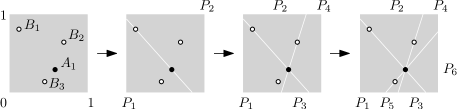
Figure 9. The inductive splitting of $S=(0,1)^{2}\smallsetminus N$ with respect to the point $A_{1}$. The points $B_{1},B_{2},B_{3}$ of $N$ are denoted as empty circles and we use a shorthand $P_{i}$ for $P_{i}(A_{1})$.

Since none of the sets $P_{i}(A_{1},\dotsc,A_{d-1})$ contains a point from $N$, it can be regarded as an intersection of $(0,1)^{d}$ with open half-spaces. Therefore every set $P_{i}(A_{1},\dotsc,A_{d-1})$ is an open convex subset of $S$. Let $P(A_{1},\dotsc,A_{d-1})$ be the set $S\smallsetminus\bigl{(}\bigcup_{B\in N}h_{A_{1},\dotsc,A_{d-1},B}\bigr{)}$. Clearly, $\lambda_{d}(P(A_{1},\dotsc,A_{d-1}))=1$. Since the sets $P_{i}(A_{1},\dotsc,A_{d-1})$ form a partitioning of $P(A_{1},\dotsc,A_{d-1})$, we also have $\sum_{i=1}^{2n}\lambda_{d}(P_{i}(A_{1},\dotsc,A_{d-1}))=1$.

For $i=1,\dotsc,2n$, we let $\mathcal{R}_{i}$ be the subset of $S^{d-1}_{*}\times S^{2}$ defined as

$$\mathcal{R}_{i}\colonequals\{(A_{1},\dotsc,A_{d+1})\in S^{d-1}_{*}\times S^{2}\colon A_{d},A_{d+1}\in P_{i}(A_{1},\dotsc,A_{d-1})\},$$

and we let $\mathcal{R}\colonequals\bigcup_{i=1}^{2n}\mathcal{R}_{i}$. The sets $\mathcal{R}_{i}$ are pairwise disjoint and it is not difficult to argue that these sets are measurable. If a $(d+1)$-tuple $(A_{1},\dotsc,A_{d+1})$ is contained in $\mathcal{R}_{i}$ for some $i\in\{1,\dotsc,2n\}$, then $(A_{1},\dotsc,A_{d+1})$ is contained in $\operatorname{Simp}_{d}(S)$, as $P_{i}(A_{1},\dotsc,A_{d-1})\cup(\operatorname{Aff}(\{A_{1},\dotsc,A_{d-1}\})\cap S)$ is a convex subset of $S$. Therefore, to find a lower bound for $\operatorname{b}_{d}(S)=\lambda_{d(d+1)}(\operatorname{Simp}_{d}(S))$, it suffices to find a lower bound for $\lambda_{d(d+1)}(\mathcal{R})$, because $\mathcal{R}$ is a subset of $\operatorname{Simp}_{d}(S)$. By Fubini’s Theorem, we obtain

$$\lambda_{d(d+1)}(\mathcal{R}_{i}) =\int_{(A_{1},\dotsc,A_{d+1})\in S^{d-1}_{*}\times S^{2}}[(A_{1},\dotsc,A_{d+1})\in\mathcal{R}_{i}]$$

$$=\int_{(A_{1},\dotsc,A_{d-1})\in S^{d-1}_{*}}\left(\int_{(A_{d},A_{d+1})\in S^{2}}[A_{d},A_{d+1}\in P_{i}(A_{1},\dotsc,A_{d-1})]\right)$$

$$=\int_{(A_{1},\dotsc,A_{d-1})\in S^{d-1}_{*}}\lambda_{d}(P_{i}(A_{1},\dotsc,A_{d-1}))^{2},$$

where $[\phi]$ is the characteristic function of a logical expression $\phi$, that is, $[\phi]$ equals $1$ if the condition $\phi$ holds and $0$ otherwise. For the measure of $\mathcal{R}$ we then derive

$$\lambda_{d(d+1)}(\mathcal{R})=\sum_{i=1}^{2n}\lambda_{d(d+1)}(\mathcal{R}_{i})=\int_{(A_{1},\dotsc,A_{d-1})\in S^{d-1}_{*}}\sum_{i=1}^{2n}\left(\lambda_{d}(P_{i}(A_{1},\dotsc,A_{d-1})\right)^{2}.$$

Since the function $x\mapsto x^{2}$ is convex, we can apply Jensen’s inequality and bound the last term from below by

$$\int_{(A_{1},\dotsc,A_{d-1})\in S^{d-1}_{*}}2n\left(\frac{\sum_{i=1}^{2n}\lambda_{d}(P_{i}(A_{1},\dotsc,A_{d-1}))}{2n}\right)^{2}=\frac{1}{2n}.\qed$$

The next step in the proof of Theorem 1.6 is to find a convenient $n$-tuple $N$ of points from $(0,1)^{d}$ whose removal produces a set with sufficiently small convexity ratio. We are going to find $N$ using a continuous version of the well-known Epsilon Net Theorem [10]. Before stating this result, we need some definitions.

Let $X$ be a subset of $\mathbb{R}^{d}$ and let $\mathcal{U}$ be a set system on $X$. We say that a set $T\subseteq X$ is shattered by $\mathcal{U}$ if every subset of $T$ can be obtained as the intersection of some $U\in\mathcal{U}$ with $T$. The Vapnik-Chervonenkis dimension (or VC-dimension) of $\mathcal{U}$, denoted by $\dim(\mathcal{U})$, is the maximum $n$ (or $\infty$ if no such maximum exists) for which some subset of $X$ of cardinality $n$ is shattered by $\mathcal{U}$.

Let $\mathcal{U}$ be a system of measurable subsets of a set $X\subseteq\mathbb{R}^{d}$ with $\lambda_{d}(X)=1$, and let $\varepsilon\in(0,1)$ be a real number. A set $N\subseteq X$ is called an $\varepsilon$-net for $(X,\mathcal{U})$ if $N\cap U\neq\emptyset$ for every $U\in\mathcal{U}$ with $\lambda_{d}(U)\geqslant\varepsilon$.

Theorem 3.4 ([14, Theorem 10.2.4]).

Let $X$ be a subset of $\mathbb{R}^{d}$ with $\lambda_{d}(X)=1$. Then for every system $\mathcal{U}$ of measurable subsets of $X$ with $\dim(\mathcal{U})\leqslant v$, $v\geqslant 2$, there is a $\frac{1}{r}$-net for $(X,\mathcal{U})$ of size at most $2vr\log_{2}r$ for $r$ sufficiently large with respect to $v$.

To apply Theorem 3.4, the VC-dimension of the set system $\mathcal{U}$ has to be finite. However, it is known that the VC-dimension of all convex sets in $\mathbb{R}^{d}$ is infinite (see e.g. [14, page 238]). Therefore, instead of considering convex sets directly, we approximate them by ellipsoids.

A $d$-dimensional ellipsoid in $\mathbb{R}^{d}$ is an image of the closed $d$-dimensional unit ball under a nonsingular affine map. A convex body in $\mathbb{R}^{d}$ is a compact convex subset of $\mathbb{R}^{d}$ with non-empty interior. The following result, known as John’s Lemma [11], shows that every convex body can be approximated by an inscribed ellipsoid.

Lemma 3.5 ([14, Theorem 13.4.1]).

For every $d$-dimensional convex body $K\subseteq\mathbb{R}^{d}$, there is a $d$-dimensional ellipsoid $E$ with the center $C$ that satisfies

$$E\subseteq K\subseteq C+d(E-C).$$

In particular, we have $\lambda_{d}(K)/d^{d}\leqslant\lambda_{d}(E)$.

As the last step before the proof of Theorem 1.6, we mention the following fact, which implies that the VC-dimension of the system $\mathcal{E}$ of $d$-dimensional ellipsoids in $\mathbb{R}^{d}$ is at most $\binom{d+2}{d}$.

Lemma 3.6 ([14, Proposition 10.3.2]).

Let $\mathbb{R}[x_{1},\dotsc,x_{d}]_{\leqslant t}$ denote the set of real polynomials in $d$ variables of degree at most $t$, and let

$$\mathcal{P}_{d,t}=\bigl{\{}\{x\in\mathbb{R}^{d}\colon p(x)\geqslant 0\}\colon p\in\mathbb{R}[x_{1},\dotsc,x_{d}]_{\leqslant t}\bigr{\}}.$$

Then $\dim(\mathcal{P}_{d,t})\leqslant\binom{d+t}{d}$.

Proof of Theorem 1.6.

Suppose we are given $\varepsilon>0$ which is sufficiently small with respect to $d$. We show how to construct a set $S\subseteq\mathbb{R}^{d}$ with $\lambda_{d}(S)=1$ satisfying $\operatorname{c}(S)\leqslant\varepsilon$ and

$$\operatorname{b}_{d}(S)\geqslant\frac{1}{8\binom{d+2}{d}d^{d}}\cdot\frac{\varepsilon}{\log_{2}{1/\varepsilon}}.$$

Without loss of generality we assume that $\varepsilon=d^{d}/r$ for some integer $r\geqslant 2d^{2d}$.

Consider the open $d$-dimensional box $(0,1)^{d}$ and the system $\mathcal{E}\restriction(0,1)^{d}$ of $d$-dimensional ellipsoids in $(0,1)^{d}$. Since the restriction of $\mathcal{E}$ to $(0,1)^{d}$ does not increase the VC-dimension, Lemma 3.6 implies $\dim(\mathcal{E}\restriction(0,1)^{d})\leqslant\binom{d+2}{d}$.

If we set $n\colonequals 2\binom{d+2}{d}r\lceil\log_{2}{r}\rceil$, then, by Theorem 3.4, there is a $\frac{1}{r}$-net $N$ for the system $((0,1)^{d},\mathcal{E}\restriction(0,1)^{d})$ of size $n$, having $r$ sufficiently large with respect to $d$. Let $S$ be the set $(0,1)^{d}\smallsetminus N$. Clearly, we have $\lambda_{d}(S)=1$.

Suppose $K$ is a convex subset of $(0,1)^{d}$ with $\lambda_{d}(K)>\varepsilon$. Since the measure of $K$ is positive, we can assume that $K$ is a convex body of measure at least $\varepsilon$. By Lemma 3.5, the convex body $K$ contains a $d$-dimensional ellipsoid $E$ with $\lambda_{d}(E)\geqslant\varepsilon/d^{d}=\frac{1}{r}$. Therefore $E\cap N\neq\emptyset$. Since we have $E\subseteq K$ and $N\cap S=\emptyset$, we see that $K$ is not a subset of $S$. In other words, we have $\operatorname{c}(S)\leqslant\varepsilon$.

By Lemma 3.3, we have $\operatorname{b}_{d}(S)\geqslant\frac{1}{2n}$. According to the choice of $n$ and $r$, the term $\frac{1}{2n}$ is bounded from below by

$$\frac{1}{4\binom{d+2}{d}r\log_{2}{2r}}=\frac{\varepsilon}{4\binom{d+2}{d}d^{d}\log_{2}{(2d^{d}/\varepsilon)}}\geqslant\frac{1}{8\binom{d+2}{d}d^{d}}\cdot\frac{\varepsilon}{\log_{2}{1/\varepsilon}},$$

where the last inequality follows from the estimate $2d^{d}\leqslant 1/\varepsilon$. This completes the proof of Theorem 1.6. ∎

It is a natural question whether the bound for $\operatorname{b}_{d}(S)$ in Theorem 1.6 can be improved to $\operatorname{b}_{d}(S)=\Omega(\operatorname{c}(S))$. In the plane, this is related to the famous problem of Danzer and Rogers (see [5, 15] and Problem E14 in [8]) which asks whether for given $\varepsilon>0$ there is a set $N^{\prime}\subseteq(0,1)^{2}$ of size $O(\frac{1}{\varepsilon})$ with the property that every convex set of area $\varepsilon$ within the unit square contains at least one point from $N^{\prime}$.

If this problem was to be answered affirmatively, then we could use such a set $N^{\prime}$ to stab $(0,1)^{2}$ in our proof of Theorem 1.6 which would yield the desired bound for $\operatorname{b}_{2}(S)$. However it is generally believed that the answer is likely to be nonlinear in $\frac{1}{\varepsilon}$.

3.3. A set with large $k$-index of convexity and small convexity ratio

Proposition 3.7.

For every integer $d\geqslant 2$, the set $S\colonequals[0,1]^{d}\smallsetminus\mathbb{Q}^{d}$ satisfies $\operatorname{c}(S)=0$ and $\operatorname{b}_{k}(S)=1$ for every positive integer $k<d$.

Proof.

Since $\mathbb{Q}^{d}$ is countable and $\lambda_{d}([0,1]^{d})=1$, we have $\lambda_{d}(S)=1$. Every convex subset $K$ of $[0,1]^{d}$ with positive $d$-dimensional measure contains an open $d$-dimensional ball $\mathfrak{B}$ with positive diameter, as there is a $(d+1)$-tuple of affinely independent points of $K$. Since $\mathbb{Q}^{d}$ is a dense subset of $\mathbb{R}^{d}$, we see that $\mathfrak{B}\cap\mathbb{Q}^{d}\neq\emptyset$ and thus $\operatorname{c}(S)=0$.

It remains to estimate $\operatorname{b}_{k}(S)$. By Fubini’s Theorem, we have

$$\operatorname{b}_{k}(S)=\int_{(B_{1},\dotsc,B_{k})\in S^{k}}\frac{\lambda_{d}\bigl{(}\{A\in S\colon\operatorname{Conv}(\{B_{1},\dotsc,B_{k},A\})\subseteq S\}\bigr{)}}{\lambda_{d}(S)^{k+1}}.$$

If $A$ is a point of $S$ such that $\operatorname{Conv}(\{B_{1},\dotsc,B_{k},A\})$ is not contained in $S$, then $A$ is a point of the affine hull $\operatorname{Aff}(\{B_{1},\dotsc,B_{k},Q\})$ of $B_{1},\dotsc,B_{k}$ and some $Q\in\mathbb{Q}^{d}$. Therefore, $\operatorname{b}_{k}(S)$ is at least

$$\int_{(B_{1},\dotsc,B_{k})\in S^{k}}\frac{\lambda_{d}([0,1]^{d})-\lambda_{d}\bigl{(}\bigcup_{Q\in\mathbb{Q}^{d}}\operatorname{Aff}(\{B_{1},\dotsc,B_{k},Q\})\bigr{)}}{\lambda_{d}(S)^{k+1}}.$$

A countable union of affine subspaces of dimension less than $d$ has $d$-dimensional measure zero and we already know that $\lambda_{d}(S)=1=\lambda_{d}([0,1]^{d})$, hence $\operatorname{b}_{k}(S)=1$. ∎

4. Other variants and open problems

We have seen in Theorem 1.3 that a p-componentwise simply connected set $S\subseteq\mathbb{R}^{2}$ whose $\operatorname{b}(S)$ is defined satisfies $\operatorname{b}(S)\leqslant\alpha\operatorname{c}(S)$, for an absolute constant $\alpha\leqslant 180$. Equivalently, such a set $S$ satisfies $\operatorname{smc}(S)\geqslant\operatorname{b}(S)\lambda_{2}(S)/180$.

By a result of Blaschke [4] (see also Sas [19]), every convex set $K\subseteq\mathbb{R}^{2}$ contains a triangle of measure at least $\frac{3\sqrt{3}}{4\pi}\lambda_{2}(K)$. In view of this, Theorem 1.3 yields the following consequence.

Corollary 4.1.

There is a constant $\alpha>0$ such that every p-componentwise simply connected set $S\subseteq\mathbb{R}^{2}$ whose $\operatorname{b}(S)$ is defined contains a triangle $T\subseteq S$ of measure at least $\alpha\operatorname{b}(S)\lambda_{2}(S)$.

A similar argument works in higher dimensions as well. For every $d\geqslant 2$, there is a constant $\beta=\beta(d)$ such that every convex set $K\subseteq\mathbb{R}^{d}$ contains a simplex of measure at least $\beta\lambda_{d}(K)$ (see e.g. Lassak [13]). Therefore, Theorem 1.5 can be rephrased in the following equivalent form.

Corollary 4.2.

For every $d\geqslant 2$, there is a constant $\alpha=\alpha(d)>0$ such that every set $S\subseteq\mathbb{R}^{d}$ whose $\operatorname{b}_{d}(S)$ is defined contains a simplex $T$ of measure at least $\alpha\operatorname{b}_{d}(S)\lambda_{d}(S)$.

What can we say about sets $S\subseteq\mathbb{R}^{2}$ that are not p-componentwise simply connected? First of all, we can consider a weaker form of simple connectivity: we call a set $S$ p-componentwise simply $\triangle$-connected if for every triangle $T$ such that $\partial T\subseteq S$ we have $T\subseteq S$. We conjecture that Theorem 1.3 can be extended to p-componentwise simply $\triangle$-connected sets.

Conjecture 4.3.

There is an absolute constant $\alpha>0$ such that every p-componentwise simply $\triangle$-connected set $S\subseteq\mathbb{R}^{2}$ whose $\operatorname{b}(S)$ is defined satisfies $\operatorname{b}(S)\leqslant\alpha\operatorname{c}(S)$.

What does the value of $\operatorname{b}(S)$ say about a planar set $S$ that does not satisfy even a weak form of simple connectivity? As Proposition 3.7 shows, such a set may not contain any convex subset of positive measure, even when $\operatorname{b}(S)$ is equal to $1$. However, we conjecture that a large $\operatorname{b}(S)$ implies the existence of a large convex set whose boundary belongs to $S$.

Conjecture 4.4.

For every $\varepsilon>0$, there is a $\delta>0$ such that if $S\subseteq\mathbb{R}^{2}$ is a set with $\operatorname{b}(S)\geqslant\varepsilon$, then there is a bounded convex set $C\subseteq\mathbb{R}^{2}$ with $\lambda(C)\geqslant\delta\lambda(S)$ and $\partial C\subseteq S$.

Theorem 1.3 shows that Conjecture 4.4 holds for p-componentwise simply connected sets, with $\delta$ being a constant multiple of $\varepsilon$. It is possible that even in the general setting of Conjecture 4.4, $\delta$ can be taken as a constant multiple of $\varepsilon$.

Motivated by Corollary 4.1, we propose a stronger version of Conjecture 4.4, where the convex set $C$ is required to be a triangle.

Conjecture 4.5.

For every $\varepsilon>0$, there is a $\delta>0$ such that if $S\subseteq\mathbb{R}^{2}$ is a set with $\operatorname{b}(S)\geqslant\varepsilon$, then there is a triangle $T\subseteq\mathbb{R}^{2}$ with $\lambda(T)\geqslant\delta\lambda(S)$ and $\partial T\subseteq S$.

Note that Conjecture 4.5 holds when restricted to p-componentwise simply connected sets, as implied by Corollary 4.1.

We can generalize Conjecture 4.5 to higher dimensions and to higher-order indices of convexity. To state the general conjecture, we introduce the following notation: for a set $X\subseteq\mathbb{R}^{d}$, let $\binom{X}{k}$ be the set of $k$-element subsets of $X$, and let the set $\operatorname{Skel}_{k}(X)$ be defined by

$$\operatorname{Skel}_{k}(X)\colonequals\bigcup_{Y\in\binom{X}{k+1}}\operatorname{Conv}(Y).$$

If $X$ is the vertex set of a $d$-dimensional simplex $T=\operatorname{Conv}(X)$, then $\operatorname{Skel}_{k}(X)$ is often called the $k$-dimensional skeleton of $T$. Our general conjecture states, roughly speaking, that sets with large $k$-index of convexity should contain the $k$-dimensional skeleton of a large simplex. Here is the precise statement.

Conjecture 4.6.

For every $k,d\in\mathbb{N}$ such that $1\leqslant k\leqslant d$ and every $\varepsilon>0$, there is a $\delta>0$ such that if $S\subseteq\mathbb{R}^{d}$ is a set with $\operatorname{b}_{k}(S)\geqslant\varepsilon$, then there is a simplex $T$ with vertex set $X$ such that $\lambda_{d}(T)\geqslant\delta\lambda_{d}(S)$ and $\operatorname{Skel}_{k}(X)\subseteq S$.

Corollary 4.2 asserts that this conjecture holds in the special case of $k=d\geqslant 2$, since $\operatorname{Skel}_{d}(X)=\operatorname{Conv}(X)=T$. Corollary 4.1 shows that the conjecture holds for $k=1$ and $d=2$ if $S$ is further assumed to be p-componentwise simply connected. In all these cases, $\delta$ can be taken as a constant multiple of $\varepsilon$, with the constant depending on $k$ and $d$.

Finally, we can ask whether there is a way to generalize Theorem 1.3 to higher dimensions, by replacing simple connectivity with another topological property. Here is an example of one such possible generalization.

Conjecture 4.7.

For every $d\geqslant 2$, there is a constant $\alpha=\alpha(d)>0$ such that if $S\subseteq\mathbb{R}^{d}$ is a set with $\operatorname{b}_{d-1}(S)$ defined whose every p-component is contractible, then $\operatorname{b}_{d-1}(S)\leqslant\alpha\operatorname{c}(S)$.

A modification of the proof of Theorem 1.5 implies that Conjecture 4.7 is true for star-shaped sets $S$.

References

- [1] Gerald A. Beer, Continuity properties of the visibility function, Michigan Math. J. 20 (4), 297–302, 1973.
- [2] Gerald A. Beer, The index of convexity and the visibility function, Pacific J. Math. 44 (1), 59–67, 1973.
- [3] Gerald A. Beer, The index of convexity and parallel bodies, Pacific J. Math. 53 (2), 337–345, 1974.
- [4] Wilhelm Blaschke, Über affine Geometrie III: Eine Minimumeigenschaft der Ellipse, Ber. Verh. Kön. Sächs. Ges. Wiss. Leipzig Math.-Phys. Kl. 69, 3–12, 1917.
- [5] Phillip G. Bradford and Vasilis Capoyleas, Weak -nets for points on a hypersphere, Discrete Comput. Geom. 18 (1), 83–91, 1997.
- [6] Sergio Cabello, Josef Cibulka, Jan Kynčl, Maria Saumell, and Pavel Valtr, Peeling potatoes near-optimally in near-linear time, in: Siu-Wing Cheng and Olivier Devillers (eds.), 30th Annual Symposium on Computational Geometry (SoCG 2014), pp. 224–231, ACM, New York, 2014.
- [7] Sergio Cabello and Maria Saumell, personal communication to Günter Rote.
- [8] Hallard T. Croft, Kenneth J. Falconer, and Richard K. Guy, Unsolved Problems in Geometry, vol. 2 of Unsolved Problems in Intuitive Mathematics, Springer, New York, 1991.
- [9] Jacob E. Goodman, On the largest convex polygon contained in a non-convex -gon, or how to peel a potato, Geom. Dedicata 11 (1), 99–106, 1981.
- [10] David Haussler and Emo Welzl, -Nets and simplex range queries, Discrete Comput. Geom. 2 (2), 127–151, 1987.
- [11] Fritz John, Extremum problems with inequalities as subsidiary conditions, in: Kurt O. Friedrichs, Otto E. Neugebauer, and James J. Stoker (eds.), Studies and Essays: Courant Anniversary Volume, pp. 187–204, Interscience Publ., New York, 1948.
- [12] Robert Lang, A note on the measurability of convex sets, Arch. Math. 47 (1), 90–92, 1986.
- [13] Marek Lassak, Approximation of convex bodies by inscribed simplices of maximum volume, Beitr. Algebra Geom. 52 (2), 389–394, 2011.
- [14] Jiří Matoušek, Lectures on Discrete Geometry, vol. 212 of Graduate Texts in Mathematics, Springer, New York, 2002.
- [15] János Pach and Gábor Tardos, Piercing quasi-rectangles—on a problem of Danzer and Rogers, J. Combin. Theory Ser. A 119 (7), 1391–1397, 2012.
- [16] Viktor V. Prasolov, Elements of Combinatorial and Differential Topology, vol. 74 of Graduate Studies in Mathematics, Amer. Math. Soc., Providence, 2006.
- [17] Günter Rote, The degree of convexity, in: 29th European Workshop on Computational Geometry (EuroCG 2013), pp. 69–72, 2013.
- [18] Walter Rudin, Real and Complex Analysis, 3rd edition, McGraw-Hill, New York, 1987.
- [19] Ernst Sas, Über eine Extremumeigenschaft der Ellipsen, Compositio Math. 6, 468–470, 1939.
- [20] Helman I. Stern, Polygonal entropy: a convexity measure, Pattern Recogn. Lett. 10 (4), 229–235, 1989.