METAL-POOR, STRONGLY STAR-FORMING GALAXIES IN THE DEEP2 SURVEY: THE RELATIONSHIP BETWEEN STELLAR MASS, TEMPERATURE-BASED METALLICITY, AND STAR FORMATION RATE

Abstract

We report on the discovery of 28 $z\approx 0.8$ metal-poor galaxies in DEEP2. These galaxies were selected for their detection of the weak [O iii]$\lambda$4363 emission line, which provides a “direct” measure of the gas-phase metallicity. A primary goal for identifying these rare galaxies is to examine whether the fundamental metallicity relation (FMR) between stellar mass, gas metallicity, and star formation rate (SFR) holds for low stellar mass and high SFR galaxies. The FMR suggests that higher SFR galaxies have lower metallicity (at fixed stellar mass). To test this trend, we combine spectroscopic measurements of metallicity and dust-corrected SFRs, with stellar mass estimates from modeling the optical photometry. We find that these galaxies are $1.05\pm 0.61$ dex above the $z\sim 1$ stellar mass–SFR relation, and $0.23\pm 0.23$ dex below the local mass–metallicity relation. Relative to the FMR, the latter offset is reduced to 0.01 dex, but significant dispersion remains (0.29 dex with 0.16 dex due to measurement uncertainties). This dispersion suggests that gas accretion, star formation and chemical enrichment have not reached equilibrium in these galaxies. This is evident by their short stellar mass doubling timescale of $\approx 100^{+310}_{-75}$ Myr that suggests stochastic star formation. Combining our sample with other $z\sim 1$ metal-poor galaxies, we find a weak positive SFR–metallicity dependence (at fixed stellar mass) that is significant at 94.4% confidence. We interpret this positive correlation as recent star formation that has enriched the gas, but has not had time to drive the metal-enriched gas out with feedback mechanisms.

1. INTRODUCTION

The chemical enrichment of galaxies, driven by star formation and modulated by gas flows from supernova and cosmic accretion, is key for understanding galaxy formation and evolution. The primary approach for measuring metal abundances is spectroscopy of nebular emission lines. These emission lines can be observed in the optical and near-infrared at $z\lesssim 3$ from the ground (e.g., Kobulnicky & Kewley, 2004; Erb et al., 2006; Maiolino et al., 2008; Hainline et al., 2009; Hayashi et al., 2009; Mannucci et al., 2009; Moustakas et al., 2011; Rigby et al., 2011; Nakajima et al., 2012; Henry et al., 2013a; Momcheva et al., 2013; Pirzkal et al., 2013; Zahid et al., 2011; Ly et al., 2014; Troncoso et al., 2014; de los Reyes et al., 2015) and space (e.g., Atek et al., 2011; van der Wel et al., 2011; Xia et al., 2012; Henry et al., 2013b; Whitaker et al., 2014b), and the James Webb Space Telescope will extend this to $z\sim 6$.

The most reliable metallicity measurements are made by measuring the flux ratio of the [O iii]$\lambda$4363 line against [O iii]$\lambda$5007. The technique is called the $T_{e}$ method because it determines the electron temperature ($T_{e}$) of the gas, and hence the gas-phase metallicity (Aller, 1984). However, the detection of [O iii]$\lambda$4363 is difficult, as it is weak, almost undetectable in metal-rich galaxies. Only 0.3% of the Sloan Digital Sky Survey (SDSS) has detected [O iii]$\lambda$4363 at signal-to-noise (S/N) $\geq 2$ (Izotov et al., 2006).

Efforts have been made to increase the number of galaxies with direct metallicities in the local universe (e.g., Brown et al., 2008; Berg et al., 2012; Izotov et al., 2012), and at $z\gtrsim 0.2$ (Hoyos et al., 2005; Kakazu et al., 2007; Hu et al., 2009; Amorín et al., 2014a, b; Ly et al., 2014, hereafter Ly14); however, the total sample size is $\sim$145 (mostly in the local universe).

Using the DEEP2 Galaxy Redshift Survey (Davis et al., 2003; Newman et al., 2013), we are conducting studies that utilize [O iii]$\lambda$4363 detections in individual galaxies and from stacked spectra. In this paper, we focus on first results from individual [O iii]$\lambda$4363 detections in 28 galaxies. Our sample of 28 galaxies substantially increases the number of $z\geq 0.25$ galaxies with S/N$\geq$3 [O iii]$\lambda$4363 detections by 44% (64 to 92).

While the selection function is biased toward metal-poor galaxies, this galaxy population is of significant interest for understanding galaxy evolution. Their low metallicity suggests that they are either (1) in their earliest stages of formation, (2) accreting metal-poor gas, or (3) undergoing significant metal-enriched gas outflows. Metal-poor galaxies have been poorly studied due to the difficulty of identifying them. Thus, the majority of previous high-$z$ metallicity studies have only used strong-line metallicity calibrations. These calibrations are problematic for high-$z$ galaxies due to suspected differences in the physical conditions of the interstellar gas (e.g., Liu et al., 2008; Kewley et al., 2013a, b), but see also Juneau et al. (2014) for a different interpretation. These differences, if present, may be incorrectly interpreted as evolution in the metal content. Thus, obtaining $T_{e}$-based metallicities at high redshifts is the next logical step, and these [O iii]$\lambda$4363 detections can potentially be used to recalibrate the strong-line diagnostics.

While the $T_{e}$ method is affected by properties of the ionized gas (e.g., optical depth, density, ionization parameter, non-equilibrium electron energy; Nicholls et al., 2014), such effects also apply to strong-line diagnostics as Nicholls et al. (2014) demonstrated. Thus, while the $T_{e}$ method is less “direct” than was initially determined (Seaton, 1954), measuring the electron temperature currently remains the preferred way to determine gas metallicities.

In this paper, we focus on the relationship between stellar mass, gas-phase metallicity, and SFR for our sample of 28 metal-poor galaxies. This relationship has received significant interest as Ellison et al. (2008) found that at a given stellar mass, lower-metallicity galaxies in the local universe tend to have higher SFRs. Thus, while the stellar mass–metallicity relation is tight ($\sim$0.1 dex; Tremonti et al., 2004), it may be a projection of a non-evolving three-dimensional relationship between stellar mass ($M_{\star}$), gas-phase metallicity ($Z$), and SFR (e.g., Lara-López et al., 2010; Mannucci et al., 2010; Hunt et al., 2012).

However, the existence of a $M_{\star}$–$Z$–SFR relation (dubbed the “fundamental metallicity relation” or “FMR”) remains controversial, as recent studies have yielded results that agree or disagree with predictions (see Salim et al. 2014 and de los Reyes et al. 2015 for a review). Moreover, the $M_{\star}$–$Z$–SFR relation has yet to be tested with large samples of metal-poor ($Z\lesssim 0.25$ $Z_{\sun}$) galaxies, especially at higher redshift. The largest high-$z$ metal-poor sample is that of Ly14 from the Subaru Deep Field (SDF; Kashikawa et al., 2004; Ly et al., 2007), which detected [O iii]$\lambda$4363 in 20 galaxies at $z\sim 0.4$–1. In this study, they found evidence that galaxies with the highest specific SFR (SFR/$M_{\star}$, hereafter sSFR) were not necessary more metal-poor. This result, based on 20 galaxies, requires further confirmation with our DEEP2 sample.

In this study, we compare our work with Andrews & Martini (2013) (hereafter AM13) who stacked $0.027<z<0.25$ SDSS spectra in bins of SFR and $M_{\star}$ to obtain average [O iii]$\lambda$4363 measurements. We note that the primary selection functions of AM13 (magnitude-limited) and our study (emission-line strengths) are different. In a forthcoming paper, we will follow the same approach as AM13 of stacking the spectra of a few thousand $z\sim$0.8 DEEP2 galaxies, allowing for a more self-consistent comparison. For now, we investigate the $M_{\star}$–$Z$–SFR relation with individual $T_{e}$ metallicity measurements. Throughout this Letter, we adopt a cosmology with $\Omega_{\Lambda}=0.7$, $\Omega_{M}=0.3$, and $h=0.7$, a Chabrier (2003) initial mass function (IMF), and a solar metallicity of 12 + $\log({\rm O/H})$ = 8.69.

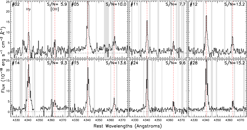
Figure 1.— Detections of [O iii]$\lambda$4363 in $z\sim 0.8$ DEEP2 galaxies. The Keck/DEIMOS spectra for 8 of 28 galaxies are shown by the solid black lines, with vertical red dashed lines indicating the locations of H$\gamma$$\lambda$4340 and [O iii]$\lambda$4363. OH skylines are indicated by the grey shaded regions. The signal-to-noise of [O iii]$\lambda$4363 detections is reported in the top right.

2. THE SAMPLE

The DEEP2 Survey has surveyed $\sim$3 deg² over four fields using the DEIMOS multi-object spectrograph (Faber et al., 2003) on the Keck-II telescope. The survey has provided optical ($\approx$6500–9000Å) spectra for $\sim$53,000 galaxies brighter than $R_{\rm AB}=24.1$, and precise redshifts for $\sim$70% of targeted galaxies. An overview of the survey can be found in Newman et al. (2013).

Using the fourth data release (DR4), we select 37,396 sources with reliable redshifts (quality flag $\geq$3). We consider those with spectral coverage that spans 3720–5010 Å (rest-frame). This enable us to determine metallicity from oxygen and hydrogen emission lines ([O ii]$\lambda\lambda$3726,3729, [O iii]$\lambda\lambda\lambda$4363,4959,5007, and H$\beta$), and further limits the sample to 4,140 galaxies at $z=0.697$–0.859 (average: 0.779).

We follow the approach of Ly14 that fits emission lines with Gaussian profiles using the IDL routine mpfit (Markwardt, 2009). Spectroscopic redshifts are used as priors for the location of emission lines. With measurements of emission-line fluxes and the noise in the spectra (measured from a 200 Å region around each line), we select those with [O iii]$\lambda$4363 and [O iii]$\lambda$5007 detected at S/N$\geq$3 and S/N$\geq$100, respectively. This yields an initial sample of 54 galaxies. We inspect each spectrum and remove 26 galaxies from our sample, primarily because of contamination from OH sky-lines. This leaves 28 galaxies. One source (#21) was observed twice. The other spectrum also detected [O iii]$\lambda$4363 at lower S/N, so the better spectrum is used in our analysis. Compared to the previous DEEP2 sample (Hoyos et al., 2005), we confirmed two, thus 26 galaxies in our sample are newly identified. Detections of [O iii]$\lambda$4363 are shown in Figure 1, and galaxy properties are provided in Table 1. We illustrate in Figure 2 the emission-line luminosities, rest-frame equivalent widths (EWs), and $O_{32}$ $\equiv$ [O iii]/[O ii] and $R_{23}$ $\equiv$ ([O ii]+[O iii])/H$\beta$ flux ratios (Pagel et al., 1979; McGaugh, 1991), and compare our sample to local galaxies and other [O iii]$\lambda$4363-detected galaxies (Ly14).

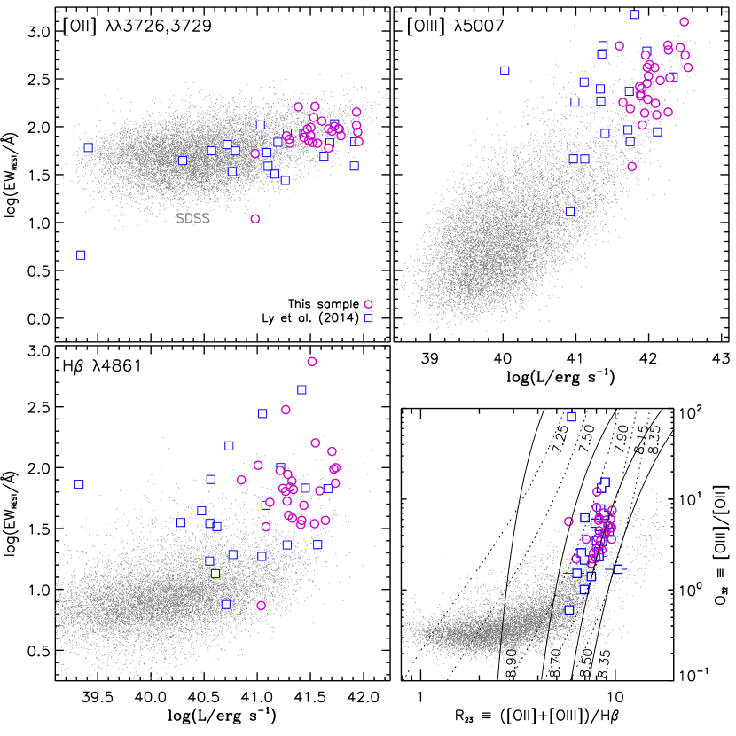
Figure 2.— Emission-line luminosities, flux ratios, and rest-frame EWs for our [O iii]$\lambda$4363 sample (purple circles). All luminosities and flux ratios are observed, before correction for dust attenuation. Gray points illustrate the SDSS DR7 emission-line sample. The lower right panel shows the metallicity-sensitive ($R_{23}$) and ionization parameter-sensitive ($O_{32}$) emission-line ratios. Photoionization models from McGaugh (1991) are overlaid for metallicities between 12 + $\log({\rm O/H})$ = 7.25 and 12 + $\log({\rm O/H})$ = 8.9. Solid (dotted) curves are for metallicities on the “upper” (“lower”) $R_{23}$ branch. Overlaid as blue squares is the [O iii]$\lambda$4363-detected sample from Ly14.

2.1. Flux Calibration

The publicly released data of DEEP2 are not flux-calibrated, which is problematic for measuring the 4363-to-5007 ratio, and hence $T_{e}$. To address this limitation, we use proprietary IDL codes developed by Jeffrey Newman, Adam Walker, and Renbin Yan of the DEEP2 team. These codes take into account the overall throughput, quantum efficiency of the eight CCD detectors, apply coarse telluric corrections for atmospheric absorption bands, and use the $R$ and $I$ DEEP2 photometry to transform the spectrum to energy units. The DEEP2 team has demonstrated that the calibration is reliable at the 10% level when compared to SDSS stars observed by DEEP2.

3. DERIVED PROPERTIES

3.1. Dust Attenuation Correction from Balmer Decrements

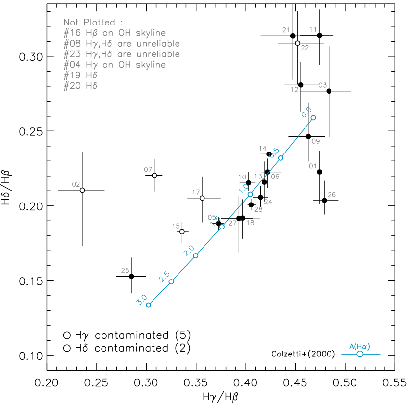
Figure 3.— Balmer decrements (H$\gamma$/H$\beta$ and H$\delta$/H$\beta$) for our [O iii]$\lambda$4363 sample. Reliable measurements are shown by the filled circles, while those affected by contamination from OH sky-line emission are shown as open circles. Blue circles and curve show the effects on the Balmer decrements with increasing dust reddening following Cal00. Values adjacent to blue circles indicate $A$(H$\alpha$). The significant scatter in the upper right is due to less reliable H$\delta$/H$\beta$ measurements. These galaxies all have H$\gamma$/H$\beta$ measurements that are consistent with $A$(H$\alpha$) $\sim 0$.

To correct the emission-line fluxes for dust attenuation, we use Balmer decrement measurements. At $z\sim 0.8$, the existing DEEP2 optical spectra measure H$\beta$, H$\gamma$, and H$\delta$. While these lines are intrinsically weak compared to H$\alpha$, our galaxies possess high emission-line EWs, which result in 22, 26, and 28 galaxies having H$\delta$, H$\gamma$, and H$\beta$ detected at S/N$\geq$10, respectively. The significant detections enable dust attenuation measurements of $\sigma$(A(H$\alpha$))$\,\approx 0.1$ mag (average from H$\gamma$/H$\beta$).

A problem encountered with Balmer emission lines is the underlying stellar absorption. Our examination of each spectrum reveal weak stellar absorption, making it difficult to obtain reliable fits to the broad wings of absorption lines. To address this limitation, we stack our spectra. Here, the continuum (around each Balmer line) is normalized to one, and an average is computed with the exclusion of spectral regions affected by OH sky-line emission. Stellar absorption is detected in H$\delta$, and is consistent with an EW_rest correction of 1 Å. For our entire sample, we adopt an EW_rest correction of 1 Å for H$\beta$, H$\gamma$, and H$\delta$. With these corrections for stellar absorption, we illustrate the Balmer decrements in Figure 3.

Assuming that the hydrogen emission originates from an optically thick H ii region obeying Case B recombination, the intrinsic Balmer flux ratios are (H$\gamma$/H$\beta$)₀ = 0.468 and (H$\delta$/H$\beta$)₀ = 0.259. Dust absorption alters these observed ratios as follows:

$$\frac{({\rm H}n/{\rm H}\beta)_{\rm obs}}{({\rm H}n/{\rm H}\beta)_{0}}=10^{-0.4E(B-V)[k({\rm H}n)-k({\rm H}\beta)]},$$ (1)

where $E$($B$–$V$) is the nebular color excess, and $k(\lambda)\equiv A(\lambda)$/$E$($B$–$V$) is the dust reddening curve. We illustrate in Figure 3 the observed Balmer decrements under the Calzetti et al. (2000) (hereafter Cal00) dust reddening formalism. We find that our Balmer decrements are consistent with Cal00. For the remainder of our Letter, all dust-corrected measurements adopt Cal00 reddening.

Our color excesses, are determined mostly (20/28) from H$\gamma$/H$\beta$. For five galaxies, we use H$\delta$/H$\beta$ since H$\gamma$ suffers from contamination from OH skylines. For the remaining 3 galaxies, the dust reddening could not be determined from either Balmer decrement (they were both affected by OH sky-line emission). For these galaxies, we assume $E(B-V)=0.22\pm 0.23$ mag ($A({\rm H}\alpha)\approx 0.73\pm 0.75$ mag), which is the average of our sample, and is consistent with other emission-line galaxy samples (e.g., Ly et al., 2012a; Domínguez et al., 2013; Momcheva et al., 2013). For Balmer decrements that imply negative reddening (6 cases), we adopt $E(B-V)=0$ with measurement uncertainties based on Balmer decrement uncertainties.

3.2. $T_{e}$-based Metallicity Determinations

To determine the gas-phase metallicity for our galaxies, we follow previous direct metallicity studies and use the empirical relations of Izotov et al. (2006). Here, we briefly summarize the approach, and refer readers to Ly14 for more details. First, the O⁺⁺ electron temperature, $T_{e}$([O iii]), can be estimated using the nebular-to-auroral [O iii] ratio, [O iii] $\lambda\lambda$4959,5007/[O iii] $\lambda$4363. We correct the above flux ratio for dust attenuation (Section 3.1). We also apply a 5% correction, since $T_{e}$ determinations from Izotov et al. (2006) are found to be overestimated (Nicholls et al., 2013).

Our [O iii] measurements have a very large dynamic range. The strongest (weakest) [O iii]$\lambda$4363 line is 6.5% (0.7%) of the [O iii] $\lambda$5007 flux. We find that the average (median) $\lambda$4363/$\lambda$5007 flux ratio for our sample is 0.018 (0.015). The derived $T_{e}$ for our galaxy sample spans (1–3.1)$\times 10^{4}$ K.

To determine the ionic abundances of oxygen, we use two emission-line flux ratios, [O ii] $\lambda\lambda$3726,3729/H$\beta$ and [O iii] $\lambda\lambda$4959,5007/H$\beta$. For our metallicity estimation, we adopt a standard two-zone temperature model with $T_{e}$([O ii]) = 0.7$T_{e}$([O iii]) + 3000 (AM13), to enable direct comparisons to local studies. In computing O⁺/H⁺, we also correct the [O ii]/H$\beta$ ratio for dust attenuation. We do not correct [O iii]/H$\beta$ since the effects are negligible.

Since the most abundant ions of oxygen in H ii regions are O⁺ and O⁺⁺, the oxygen abundances are given by ${\rm O/H}=({\rm O}^{+}+{\rm O}^{++})/{\rm H}^{+}$. In Table 1, we provide estimates of $T_{e}$([O iii]), and de-reddened metallicity for our sample. Our most metal-poor systems are #04 and #08, and can be classified as extremely metal-poor galaxies ($\leq$0.1 $Z_{\sun}$).

3.3. Dust-Corrected Star Formation Rates

In addition to gas-phase metallicity, our data allow us to determine dust-corrected SFRs using the hydrogen recombination lines, which are sensitive to the shortest timescale of star formation, $\lesssim$10 Myr.

Assuming a Chabrier (2003) IMF with masses of 0.1–100 $M_{\sun}$, and solar metallicity, the SFR can be determined from the observed H$\beta$ luminosity (Kennicutt, 1998):

$$\frac{{\rm SFR}}{M_{\sun}~{}{\rm yr}^{-1}}=4.4\times 10^{-42}\times 2.86\times 10^{0.4A({\rm H}\beta)}\frac{L({\rm H}\beta)}{{\rm erg~{}s}^{-1}},$$ (2)

where $A({\rm H}\beta)=4.6$$E$($B$–$V$). This relation overestimates the SFR at low metallicities due to the dependence of a stronger ionizing radiation field on lower metallicity. Since our galaxies have $Z\approx 0.2Z_{\sun}$, we reduce the SFRs by 37% (Henry et al., 2013b). Our SFR estimates are summarized in Table 1 and are illustrated in Figure 5. We find that our galaxies have dust-corrected SFRs of 0.8–130 $M_{\sun}$ yr^-1 with an average (median) of 10.7 (4.6) $M_{\sun}$ yr^-1.

3.4. Stellar Masses from SED Modeling

To determine stellar masses, we follow the common approach of modeling the spectral energy distribution (SED) with stellar synthesis models (e.g., Salim et al., 2007; Ly et al., 2011, 2012b). The eight-band photometric data include $BRI$ imaging from the Canada-France-Hawaii Telescope (CFHT) for the DEEP2 survey (Coil et al., 2004). In addition, publicly available $ugriz$ imaging from the CFHT Legacy Survey is available in Field #1 (Extended Groth Strip), and Fields #3–4 are located in the SDSS deep survey strip (Stripe 82) for $u\arcmin g\arcmin r\arcmin i\arcmin z\arcmin$ imaging. Thus, 18 of 27 galaxies have eight optical imaging bands. These photometric data that we use have been compiled by Matthews et al. (2013). While our galaxies have low stellar masses (as demonstrated below), the imaging data are fairly deep. The $R$-band imaging, for example, reaches an 8$\sigma$ AB limit of 24.5 (Newman et al., 2013), and our galaxies are on average 1.2 AB mag brighter than this limit.

To extend the wavelength coverage, we cross-matched our sample against the catalog of Bundy et al. (2006), which contains $JK$ photometry. Unfortunately, only two galaxies have a match. This is not a surprise since many of our galaxies have low stellar masses. While photometric data redward of 5500Å are unavailable, Zahid et al. (2011) demonstrated that stellar mass estimates from $BRI$ photometry are consistent with those obtained from $BRIK_{s}$, suggesting that the existing optical data are sufficient for stellar mass estimates. We also note that the lack of $ugriz$ imaging does not significantly hamper out SED modeling for 9 galaxies, as we compared stellar mass estimates derived from $BRI$-only and $BRI$+$ugriz$ photometry for two-thirds of our sample, and find consistent results. Future efforts will include acquiring Spitzer infrared data to provide more robust stellar mass estimates.

To model the SED, we use the Fitting and Assessment of Synthetic Templates code (Kriek et al., 2009) with Bruzual & Charlot (2003) models and adopt a Chabrier (2003) IMF, exponentially-declining star formation histories (SFHs; i.e., $\tau$ models), one-fifth solar metallicity, and Cal00 reddening. We also correct the broad-band photometry for the contribution of nebular emission lines following the approach described in Ly14. This correction reduces the stellar mass estimates by 0.2 dex (average). To determined stellar mass uncertainties, we conduct Monte Carlo realizations within FAST. Here, data points are randomly perturbed 100 times (based on the photometric uncertainties) and the SEDs are re-fitted, yielding a probability distribution function for stellar mass. The stellar masses are provided in Table 1 and are illustrated in Figures 4–5. The average (median) stellar masses are $4.9\times 10^{8}$ $M_{\sun}$ ($5.0\times 10^{8}$ $M_{\sun}$) and span $7.1\times 10^{7}$–$2.2\times 10^{9}$ $M_{\sun}$.

4. RESULTS

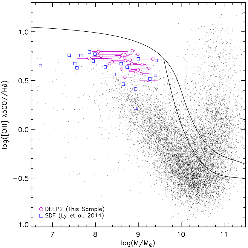
Figure 4.— [O iii]/H$\beta$ flux ratio (“excitation”) as a function of stellar mass (i.e., the MEx diagram; Juneau et al., 2014). The DEEP2 [O iii]$\lambda$4363 sample is shown by the purple circles. Overlaid as blue squares is the Ly14 [O iii]$\lambda$4363 sample from the SDF. The SDSS DR7 sample is illustrated in black.

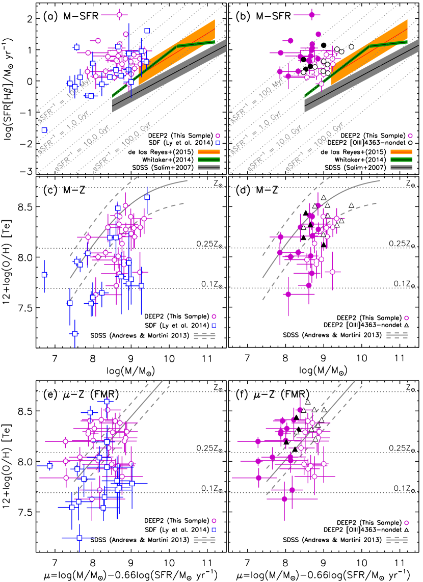
Figure 5.— Relations between stellar mass and (top) dust-corrected H$\beta$ SFR, (middle) metallicity, and (bottom) metallicity and dust-corrected H$\beta$ SFR (i.e., the FMR). The DEEP2 [O iii]$\lambda$4363 sample is shown by the purple circles. Overlaid as blue squares on the left panels is the Ly14 [O iii]$\lambda$4363 sample from the SDF. Results from the SDSS sample (Salim et al. 2007; AM13) is illustrated in gray. For comparisons, we also overlay in the top panels the stellar mass–SFR relation of H$\alpha$-selected galaxies at $z=0.8$ (de los Reyes et al., 2015) and mass-selected star-forming galaxies at $z=0.5$–1 (Whitaker et al., 2014a) in orange and green, respectively. For direct metallicity comparisons, we illustrate the results of AM13, which stacked spectra to measure average $T_{e}$-based metallicities. DEEP2 galaxies with reliable non-detections of [O iii]$\lambda$4363 are shown as black circles and triangles (lower limit on metallicity). The DEEP2 samples are separated by low and high SFRs (see text) as open and filled symbols, respectively.

4.1. Excitation Properties

Figure 4 illustrates the [O iii]$\lambda$5007/H$\beta$ flux ratios and stellar masses along the “Mass–Excitation” (MEx; Juneau et al., 2014) diagram. The MEx is used as a substitute for the Baldwin et al. (1981) diagnostic diagram when [N ii]$\lambda$6583/H$\alpha$ is unavailable. It can be seen that these galaxies have high [O iii]/H$\beta$ ratios, $5.0\pm 0.9$. All of them are classified as star-forming galaxies by falling below the solid black line. Compared to other metal-poor galaxies (blue squares Ly14), the DEEP2 galaxies have similar excitation properties, but are $\approx$0.4 dex more massive. Compared to UV- and mass-selected $z\sim 2$ galaxies (e.g., Shapley et al., 2014; Steidel et al., 2014), our measured [O iii]/H$\beta$ ratios are higher by a factor of 1.25–2.5. Their strong-line oxygen ratios, $R_{23}$ and $O_{32}$, are consistent with $z\sim 2$ galaxies from Shapley et al. (2014).

4.2. Relationship between Mass, Metallicity, and SFR

Figure 5(a) compares the dust-corrected instantaneous SFRs against the stellar mass estimates. Here we compare our work against mass-selected galaxies at $z\sim 1$ (Whitaker et al., 2014b) and H$\alpha$-selected galaxies at $z\approx 0.8$ (de los Reyes et al., 2015). Our galaxies are located $1.05\pm 0.61$ dex above these $M_{\star}$–SFR relations with SFR/$M_{\star}$ of 10^-8.0±0.6 yr^-1. This significant SFR offset is also seen for metal-poor galaxies from Ly14. By requiring [O iii]$\lambda$4363 detections, both [O iii]$\lambda$4363 studies are biased toward high-EW emission lines (see Figure 2), which correspond to a higher sSFRs.

Figure 5(c) illustrates the $M_{\star}$–$Z$ relation. Here we compare our results against AM13. It demonstrates that while a subset of our galaxies is consistent with AM13, a significant fraction (60%) are located below the relation at more than 0.22 dex (1$\sigma$; AM13, ), by as much as –0.76 dex. This results in an average $Z$ offset for the sample of –$0.28\pm 0.23$ dex. Our $M_{\star}$–$Z$ relation result is consistent with Ly14 (blue squares), who also found that half of their sample falls below the local $M_{\star}$–$Z$ relation.

The FMR was introduced to describe the dependence between $M_{\star}$, $Z$, and SFR in local galaxies, and was extended to explain higher redshift galaxies. Mannucci et al. (2010) was one of the first studies to parameterize this dependence by considering a combination of stellar mass and SFR:

$$\mu=\log{(M_{\star})}-\alpha\log{(\rm SFR)},$$ (3)

where $\alpha$ is the coefficient that minimizes the scatter against metallicity. Figure 5(e) illustrates the $\mu$ projection of the $M_{\star}$–$Z$–SFR relation with $\alpha=0.66$ (AM13). It can be seen that our sample is consistent ($0.01\pm 0.29$ dex) with the local FMR; however significant dispersion remains. The dispersion is greater than our $M_{\star}$–$Z$ comparison and the average measurement uncertainties of $\approx$0.16 dex with respect to the FMR.

The local $M_{\star}$–$Z$–SFR relation suggests that higher SFR galaxies have lower metallicity at fixed stellar mass. To examine if this is correct, we split our sample by high and low sSFRs, and perform Kolmogorov-Smirnoff (K-S) tests to determine if these two distributions are different. These two samples are illustrated in panels (b), (d) and (f) in Figure 5 as filled (high-SFR) and open (low-SFR) symbols. The sample is divided at the median $\Delta[\log({\rm SFR})]$, which is the amount of deviation relative to the Whitaker et al. (2014a) $M_{\star}$–SFR relation. This relative SFR offset follows the non-parametric approach of Salim et al. (2014).

One concern with conducting a K-S test is the selection bias of requiring the detection of [O iii]$\lambda$4363. More specifically, detection of this line primarily depends on the electron temperature (or gas metallicity), which corresponds to the $\lambda$5007/$\lambda$4363 line ratio, and the dust-corrected SFR, which determines the overall normalization of the emission-line strengths. At high SFRs, the probability of detecting [O iii]$\lambda$4363 is greater for a wide range of metallicity. This range of metallicity reduces toward lower metallicity such that only metal-poor galaxies with low SFRs can be detected in an emission-line flux limited survey.

This selection bias is demonstrated in Figure 6, which illustrates the gas-phase metallicity as a function of dust-corrected SFR. The black curves correspond to the average [O iii]$\lambda$4363 S/N=3 detection limit of $3.4\times 10^{-18}$ erg s^-1 cm^-2. This limit was determined from measuring the rms in 4,140 spectra in areas adjacent to where [O iii]$\lambda$4363 is expected to be detected. In determining the metallicity–SFR dependence, we consider (1) an ionic oxygen abundance ratio (O⁺⁺/O⁺) of unity, which is the average for our DEEP2 [O iii]$\lambda$4363 sample, and (2) a temperature–metallicity relation of 12 + $\log({\rm O/H})$ = 9.51 - 1.03($T_{e}$/10⁴ K). The latter is empirically determined from our DEEP2 [O iii]$\lambda$4363 galaxies.

To account for the $Z$–SFR selection bias, we include reliable [O iii]$\lambda$4363 non-detections within our K-S analyses. First, we consider all DEEP2 galaxies with S/N$\geq$100 on [O iii]$\lambda$5007 and a non-detection (S/N$<$3) on [O iii]$\lambda$4363. This sample of 126 galaxies is then vetted for unreliable limits because the [O iii]$\lambda$4363 emission line either falls on an OH skyline, the atmospheric A-band, or a CCD gap. This limited the sample to 79 galaxies. While the above [O iii]$\lambda$5007 S/N cut is strict, for many of these galaxies, a strong lower limit on the metallicity is not available. This is because a S/N=100 corresponds roughly to 0.03 on $\lambda$4363/$\lambda$5007 or $T_{e}$ $\approx 2\times 10^{4}$ K. Thus, we further restrict our non-detection sample to 13 galaxies with [O iii]$\lambda$5007 S/N$\geq$200. These galaxies are overlaid in Figure 6 and panels (b), (d), and (f) in Figure 5 as either black circles or black triangles (S/N=3 lower limit on metallicity). It can be seen that the majority of these galaxies are located to the left of the S/N=3 line for E(B-V) = 0.22 mag in Figure 6. Also, Figure 5 illustrates that these galaxies have higher stellar masses (0.3 dex) than our detected sample, and lower SFRs at a given stellar mass. As expected, these galaxies have higher metallicity with lower limits above 12 + $\log({\rm O/H})$ $\approx 8.2$ (average: 8.37).

For our K-S tests, we compare the $\log({\rm O/H})$ distributions for the low- and high-SFR samples, finding that these two distributions are similar with the lower SFR galaxies having slightly higher metallicity (see Figure 7(a)). However, as Figure 5(b) shows, these two samples differ in stellar mass by $\approx$0.5 dex. If instead we consider the relative offset in metallicity against the $M_{\star}$–$Z$ relation of AM13, the K-S test finds that the two samples are different at 94.4% (1.9$\sigma$; Figure 7(b)). The difference, however, is in the opposite direction of local predictions, with higher sSFR galaxies having higher gas-phase metallicities.

Given this discrepancy, it is also important to investigate whether the same result is seen when considering the FMR that Mannucci et al. (2010) defined. Here, they utilized the $R_{23}$ strong-line diagnostic and a fourth-order polynomial for $R_{23}$–$Z$ (Maiolino et al., 2008). However, the majority of our DEEP2 sample have dust-corrected $R_{23}$ values that exceed the maximum threshold value of $R_{23}=8.65$. Thus, it is not possible to conduct the same K-S test analysis with $R_{23}$ and the Maiolino et al. (2008) calibration.

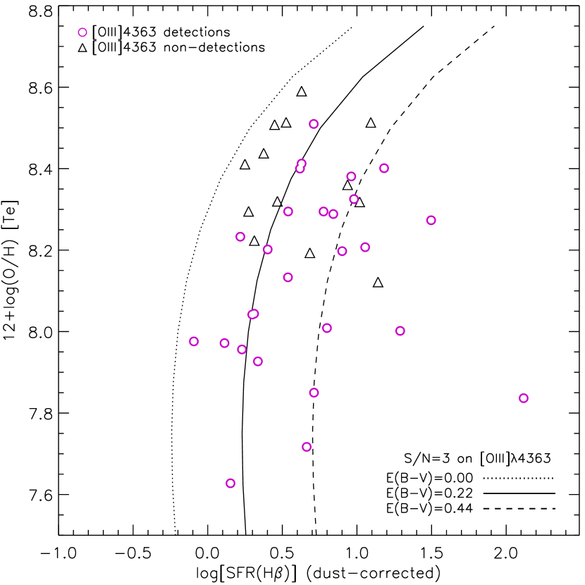
Figure 6.— Gas-phase metallicity as a function of dust-corrected SFR for our [O iii]$\lambda$4363 sample (purple circles) and a sample of reliable [O iii]$\lambda$4363 non-detections at S/N$<$3 (black triangles). The triangles are lower limits on metallicity. The dotted, solid, and dashed lines correspond to a S/N=3 limit on [O iii]$\lambda$4363 of $3.4\times 10^{-18}$ erg s^-1 cm^-2 for three dust extinction possibilities, E(B-V) = 0.0, 0.22, and 0.44, respectively. These extinction values span the dispersion seen in our sample.

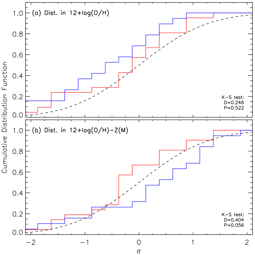
Figure 7.— Cumulative distribution functions in (a) metallicity and (b) metallicity relative to the AM13 $M_{\star}$–$Z$ relation, for two samples with low (red line) and high SFRs (blue line). The K-S statistics (D) and the probability that the two distributions are identical (P) are given in the lower right-hand corner. Panel (b) shows that the two distributions are different at 94.4% confidence.

5. DISCUSSIONS

From DEEP2 spectra of 28 galaxies with oxygen abundances from [O iii]$\lambda$4363 detections (i.e., the $T_{e}$ method), we find that metal-poor strongly star-forming galaxies are consistent with the local FMR (AM13), albeit with large dispersion (0.29 dex with 0.16 dex due to measurement errors). This result is consistent with metal-poor galaxies from Ly et al. (2014), and lensed low-mass star-forming galaxies at $z\sim$0.8–2.6 (Wuyts et al., 2012). Given the high sSFRs of $\sim$(100 Myr)^-1, we argue that the large dispersion in metallicity is unsurprising—these galaxies are most likely undergoing episodic star formation and have not settled into a steady state.

We find marginal (94.4%; 1.9$\sigma$) evidence that galaxies with higher sSFRs ($\lesssim$10^-8 yr^-1) are more metal-rich. While this contradicts previous local studies, the inverse of the sSFR—timescale for star formation—is short. Assuming outflow velocities comparable to virial velocities ($\sim$150 km s^-1) for $\log{(M_{\rm halo}/M_{\sun})}\approx 11.1$ (Behroozi et al., 2010), 8 galaxies in our sample would not have enough time (sSFR${}^{-1}\lesssim 10^{7.65}$ yr) for any recently enriched outflows to be driven out of the 1″ (7.5 kpc) slit-widths. Thus, one would expect the SFR–$Z$ dependence to turn positive for low-mass strongly star-forming galaxies. Given the instantaneous SFRs, we find that the measured oxygen abundances can be explained with low nucleosynthesis yields ($y\sim 0.01$), gas-to-stellar mass fraction of $\approx 1\pm 0.4$, and no metal loss due to outflows.

Table 1Summary of DEEP2 Sample

ID	R.A.	Declination	$z$	EW(H$\beta$)	$\log(M_{\star}/M_{\sun})$	$\log\left[\frac{{\rm SFR}_{{\rm H}\beta}}{M_{\sun}~{}{\rm yr}^{-1}}\right]$	$E$($B$–$V$)	S/N	[O ii]/H$\beta$	[O iii]/H$\beta$	$\frac{[{\rm O}\,\textsc{iii}]}{[{\rm O}\,\textsc{iii}]\lambda 4363}$	$\log(T_{e}/{\rm K})$	12 + $\log({\rm O/H})$
	(hh:mm:ss)	(dd:mm:ss)		(Å)			(mag)	($\lambda$4363)
01	14:18:31.260	52:49:42.545	0.8194	string38.46	8.81${}^{+0.18}_{-0.00}$	0.23$\pm$0.16	0.00${}^{+0.09}_{-0.08}$	4.9	2.165${}^{+0.101}_{-0.051}$	5.507${}^{+0.156}_{-0.067}$	57.273${}^{+11.748}_{-08.811}$	4.18$\pm$0.04	7.96${}^{+0.11}_{-0.14}$
02	14:21:21.513	53:01:07.672	0.7496	string51.94	8.76${}^{+0.04}_{-0.06}$	0.54${}^{+0.45}_{-0.33}$	0.28${}^{+0.24}_{-0.18}$	5.9	1.821${}^{+0.705}_{-0.235}$	7.792${}^{+0.200}_{-0.351}$	67.843${}^{+19.856}_{-06.619}$	4.14$\pm$0.04	8.13$\pm$0.10
03	14:21:25.487	53:09:48.071	0.7099	104.49	8.94${}^{+0.00}_{-0.15}$	-0.09${}^{+0.19}_{-0.25}$	0.00${}^{+0.10}_{-0.14}$	3.7	2.413$\pm$0.103	5.178${}^{+0.198}_{-0.085}$	54.985${}^{+20.947}_{-10.473}$	4.17${}^{+0.06}_{-0.05}$	7.98${}^{+0.17}_{-0.19}$
04	14:22:03.718	53:25:47.766	0.7878	string7.38	…	-0.06${}^{+0.63}_{-0.59}$	0.00${}^{+0.34}_{-0.32}$	5.5	0.867$\pm$0.094	7.273${}^{+0.385}_{-0.578}$	18.192${}^{+05.923}_{-01.692}$	4.49${}^{+0.08}_{-0.07}$	7.35${}^{+0.11}_{-0.17}$
05	14:21:45.408	53:23:52.699	0.7710	string74.51	8.86${}^{+0.07}_{-0.00}$	1.50${}^{+0.07}_{-0.05}$	0.47${}^{+0.04}_{-0.03}$	10.0	1.960$\pm$0.084	8.497${}^{+0.080}_{-0.053}$	90.482${}^{+10.167}_{-08.133}$	4.10$\pm$0.02	8.27${}^{+0.07}_{-0.06}$
06	16:47:26.188	34:45:12.126	0.7166	string36.91	8.85${}^{+0.12}_{-0.01}$	0.71${}^{+0.07}_{-0.10}$	0.21${}^{+0.04}_{-0.05}$	5.0	2.539${}^{+0.221}_{-0.095}$	6.245$\pm$0.081	131.237${}^{+47.723}_{-15.908}$	4.02${}^{+0.02}_{-0.03}$	8.51${}^{+0.13}_{-0.10}$
07	16:46:35.420	34:50:27.928	0.7624	string34.71	9.07${}^{+0.19}_{-0.00}$	0.84${}^{+0.12}_{-0.10}$	0.22${}^{+0.07}_{-0.05}$	3.4	3.304${}^{+0.208}_{-0.260}$	5.003${}^{+0.040}_{-0.081}$	83.493${}^{+25.690}_{-12.845}$	4.09$\pm$0.05	8.29${}^{+0.15}_{-0.21}$
08	16:47:26.488	34:54:09.770	0.7653	string79.33	8.07${}^{+0.69}_{-0.14}$	0.15$\pm$0.42	0.22$\pm$0.23	4.0	1.412${}^{+0.779}_{-0.097}$	7.866${}^{+0.589}_{-0.168}$	24.249${}^{+08.434}_{-04.217}$	4.38${}^{+0.08}_{-0.11}$	7.63${}^{+0.17}_{-0.21}$
09	16:49:51.368	34:45:18.210	0.7909	string53.06	9.00${}^{+0.08}_{-0.32}$	0.22${}^{+0.17}_{-0.12}$	0.02${}^{+0.09}_{-0.07}$	3.6	2.496${}^{+0.197}_{-0.079}$	5.485${}^{+0.124}_{-0.099}$	78.655${}^{+29.964}_{-14.982}$	4.10${}^{+0.05}_{-0.04}$	8.23${}^{+0.16}_{-0.17}$
10	16:51:31.472	34:53:15.964	0.7945	string64.52	8.70${}^{+0.15}_{-0.31}$	1.06$\pm$0.08	0.31$\pm$0.04	6.4	2.159${}^{+0.093}_{-0.140}$	6.739${}^{+0.094}_{-0.040}$	85.109${}^{+15.474}_{-12.379}$	4.11${}^{+0.02}_{-0.03}$	8.21${}^{+0.09}_{-0.08}$
11	16:50:55.342	34:53:29.875	0.7980	string94.85	8.56${}^{+0.21}_{-0.59}$	0.11${}^{+0.16}_{-0.11}$	0.00${}^{+0.08}_{-0.06}$	7.7	2.086$\pm$0.065	7.480${}^{+0.148}_{-0.118}$	58.301${}^{+03.195}_{-11.181}$	4.19$\pm$0.03	7.97${}^{+0.06}_{-0.11}$
12	16:53:03.486	34:58:48.946	0.7488	string69.05	8.33${}^{+0.16}_{-0.08}$	0.31${}^{+0.10}_{-0.15}$	0.06${}^{+0.05}_{-0.08}$	13.2	1.702${}^{+0.229}_{-0.000}$	6.384${}^{+0.130}_{-0.056}$	70.872${}^{+04.765}_{-05.956}$	4.15${}^{+0.02}_{-0.01}$	8.04${}^{+0.03}_{-0.05}$
13	16:51:24.060	35:01:38.740	0.7936	string32.65	9.09${}^{+0.09}_{-0.35}$	0.40${}^{+0.17}_{-0.12}$	0.23${}^{+0.09}_{-0.06}$	5.2	2.862${}^{+0.369}_{-0.185}$	6.241${}^{+0.154}_{-0.103}$	74.343${}^{+15.250}_{-11.437}$	4.13${}^{+0.03}_{-0.04}$	8.20${}^{+0.12}_{-0.11}$
14	16:51:20.343	35:02:32.628	0.7936	135.97	8.68${}^{+0.50}_{-0.30}$	0.98${}^{+0.08}_{-0.06}$	0.21$\pm$0.04	9.3	2.173$\pm$0.089	7.209$\pm$0.040	105.147${}^{+12.086}_{-09.669}$	4.07${}^{+0.01}_{-0.02}$	8.33$\pm$0.06
15	23:27:20.369	00:05:54.762	0.7553	741.71	8.13${}^{+0.01}_{-0.21}$	1.29${}^{+0.09}_{-0.10}$	0.48$\pm$0.05	13.6	1.034${}^{+0.096}_{-0.027}$	7.428${}^{+0.084}_{-0.042}$	72.096${}^{+04.614}_{-06.921}$	4.15${}^{+0.01}_{-0.02}$	8.00${}^{+0.04}_{-0.05}$
16	23:27:43.140	00:12:42.832	0.7743	string34.15	9.23${}^{+0.22}_{-0.20}$	0.71$\pm$0.42	0.22$\pm$0.23	3.4	1.958${}^{+0.945}_{-0.000}$	4.320$\pm$0.124	46.844${}^{+18.738}_{-12.492}$	4.21$\pm$0.07	7.85${}^{+0.20}_{-0.18}$
17	23:27:29.854	00:14:20.439	0.7637	string40.62	8.39${}^{+0.37}_{-0.01}$	0.78$\pm$0.19	0.32$\pm$0.10	4.3	2.420${}^{+0.596}_{-0.074}$	6.508${}^{+0.147}_{-0.074}$	89.583${}^{+28.898}_{-17.339}$	4.09$\pm$0.04	8.29${}^{+0.13}_{-0.15}$
18	23:27:07.500	00:17:41.503	0.7885	string49.03	9.34${}^{+0.21}_{-0.29}$	0.96${}^{+0.14}_{-0.17}$	0.34${}^{+0.08}_{-0.09}$	4.4	1.794${}^{+0.129}_{-0.194}$	7.022$\pm$0.113	115.500${}^{+37.258}_{-14.903}$	4.04$\pm$0.04	8.38${}^{+0.10}_{-0.15}$
19	23:26:55.430	00:17:52.919	0.8562	string97.37	8.99${}^{+0.00}_{-0.07}$	0.62${}^{+0.13}_{-0.08}$	0.00${}^{+0.07}_{-0.04}$	5.2	1.636${}^{+0.021}_{-0.026}$	7.989${}^{+0.066}_{-0.132}$	128.952${}^{+17.993}_{-23.991}$	4.04${}^{+0.03}_{-0.02}$	8.40${}^{+0.08}_{-0.13}$
20	23:30:57.949	00:03:38.191	0.7842	string87.95	8.61${}^{+0.07}_{-0.28}$	0.66${}^{+0.18}_{-0.26}$	0.26${}^{+0.10}_{-0.14}$	4.1	2.017${}^{+0.276}_{-0.221}$	5.575${}^{+0.132}_{-0.159}$	36.499${}^{+14.600}_{-05.840}$	4.26${}^{+0.05}_{-0.09}$	7.72${}^{+0.14}_{-0.19}$
21	23:31:50.728	00:09:39.393	0.8225	string63.83	8.81${}^{+0.06}_{-0.52}$	0.34${}^{+0.29}_{-0.30}$	0.09${}^{+0.16}_{-0.17}$	5.0	1.692${}^{+0.344}_{-0.115}$	6.989${}^{+0.179}_{-0.223}$	52.462${}^{+11.343}_{-08.507}$	4.19${}^{+0.05}_{-0.04}$	7.93${}^{+0.10}_{-0.14}$
22	02:27:48.871	00:24:40.077	0.7838	298.74	7.85${}^{+0.45}_{-0.06}$	0.30${}^{+0.16}_{-0.23}$	0.07${}^{+0.09}_{-0.13}$	5.3	1.735${}^{+0.343}_{-0.043}$	7.110${}^{+0.103}_{-0.207}$	61.688${}^{+12.654}_{-09.490}$	4.16${}^{+0.03}_{-0.04}$	8.04${}^{+0.10}_{-0.12}$
23	02:27:05.706	00:25:21.865	0.7661	string77.52	8.63${}^{+0.07}_{-0.18}$	0.63$\pm$0.42	0.22$\pm$0.23	3.2	1.492${}^{+0.720}_{-0.000}$	7.631${}^{+0.135}_{-0.108}$	144.017${}^{+00.000}_{-57.607}$	4.05${}^{+0.05}_{-0.06}$	8.41${}^{+0.12}_{-0.20}$
24	02:27:30.457	00:31:06.391	0.7214	159.58	7.87${}^{+0.52}_{-0.29}$	0.90${}^{+0.07}_{-0.06}$	0.25$\pm$0.04	9.6	1.525$\pm$0.076	7.105$\pm$0.057	94.916${}^{+08.344}_{-10.430}$	4.09$\pm$0.02	8.20${}^{+0.05}_{-0.06}$
25	02:26:03.707	00:36:22.460	0.7888	string66.11	8.69${}^{+0.22}_{-0.48}$	2.12${}^{+0.20}_{-0.17}$	1.02${}^{+0.11}_{-0.09}$	6.6	2.857${}^{+0.269}_{-0.336}$	4.878${}^{+0.130}_{-0.065}$	48.598${}^{+05.116}_{-08.526}$	4.23${}^{+0.04}_{-0.03}$	7.84${}^{+0.10}_{-0.09}$
26	02:26:21.479	00:48:06.813	0.7743	string36.94	9.24${}^{+0.08}_{-0.29}$	0.54$\pm$0.10	0.00${}^{+0.05}_{-0.06}$	6.7	2.064${}^{+0.031}_{-0.041}$	5.895${}^{+0.089}_{-0.044}$	109.091$\pm$14.307	4.07$\pm$0.02	8.29${}^{+0.08}_{-0.10}$
27	02:29:33.654	00:26:08.023	0.7294	string67.55	8.66${}^{+0.20}_{-0.67}$	0.80${}^{+0.14}_{-0.20}$	0.36${}^{+0.08}_{-0.11}$	7.0	2.555${}^{+0.220}_{-0.330}$	7.849${}^{+0.132}_{-0.231}$	54.969${}^{+09.644}_{-07.715}$	4.19$\pm$0.04	8.01${}^{+0.09}_{-0.12}$
28	02:29:02.031	00:30:08.127	0.7315	string99.97	8.70${}^{+0.01}_{-0.06}$	1.18${}^{+0.03}_{-0.04}$	0.30$\pm$0.02	15.2	1.515${}^{+0.042}_{-0.028}$	7.633${}^{+0.037}_{-0.019}$	132.444${}^{+10.667}_{-05.333}$	4.04$\pm$0.01	8.40${}^{+0.04}_{-0.03}$

Note. — Unless otherwise specified, [O iii] refers to [O iii]$\lambda\lambda$4959,5007.

References

- Aller (1984) Aller, L. H. 1984, Astrophysics and Space Science Library, (Dordrecht: Reidel)
- Amorín et al. (2014a) Amorín, R., Pérez-Montero, E., Contini, T., et al. 2014a, A&A, submitted (arXiv:1403.3441)
- Amorín et al. (2014b) Amorín, R., Sommariva, V., Castellano, M., et al. 2014b, A&A, 568, LL8
- Andrews & Martini (2013) Andrews, B. H., & Martini, P. 2013, ApJ, 765, 140 [AM13]
- Atek et al. (2011) Atek, H., Siana, B., Scarlata, C., et al. 2011, ApJ, 743, 121
- Baldwin et al. (1981) Baldwin, A., Phillips, M. M., & Terlevich, R. 1981, PASP, 93, 817
- Berg et al. (2012) Berg, D. A., Skillman, E. D., Marble, A. R., et al. 2012, ApJ, 754, 98
- Behroozi et al. (2010) Behroozi, P. S., Conroy, C., & Wechsler, R. H. 2010, ApJ, 717, 379
- Brown et al. (2008) Brown, W. R., Kewley, L. J., & Geller, M. J. 2008, AJ, 135, 92
- Bruzual & Charlot (2003) Bruzual, G., & Charlot, S. 2003, MNRAS, 344, 1000
- Bundy et al. (2006) Bundy, K., Ellis, R. S., Conselice, C. J., et al. 2006, ApJ, 651, 120
- Calzetti et al. (2000) Calzetti, D., Armus, L., Bohlin, R. C., Kinney, A. L., Koornneef, J., & Storchi-Bergmann, T. 2000, ApJ, 533, 682 [Cal00]
- Chabrier (2003) Chabrier, G. 2003, PASP, 115, 763
- Coil et al. (2004) Coil, A. L., Newman, J. A., Kaiser, N., et al. 2004, ApJ, 617, 765
- Davé et al. (2011) Davé, R., Finlator, K., & Oppenheimer, B. D. 2011, MNRAS, 416, 1354
- Davis et al. (2003) Davis, M., Faber, S. M., Newman, J., et al. 2003, Proc. SPIE, 4834, 161
- de los Reyes et al. (2015) de los Reyes, M., Ly, C., Lee, J. C., 2015, AJ, 149, 79
- Domínguez et al. (2013) Domínguez, A., Siana, B., Henry, A. L., et al. 2013, ApJ, 763, 145
- Ellison et al. (2008) Ellison, S. L., Patton, D. R., Simard, L., & McConnachie, A. W. 2008, ApJ, 672, L107
- Erb et al. (2006) Erb, D. K., Shapley, A. E., Pettini, M., et al. 2006, ApJ, 644, 813
- Faber et al. (2003) Faber, S. M., Phillips, A. C., Kibrick, R. I., et al. 2003, Proc. SPIE, 4841, 1657
- Hainline et al. (2009) Hainline, K. N., Shapley, A. E., Kornei, K. A., et al. 2009, ApJ, 701, 52
- Hayashi et al. (2009) Hayashi, M., Motohara, K., Shimasaku, K., et al. 2009, ApJ, 691, 140
- Henry et al. (2013a) Henry, A., Martin, C. L., Finlator, K., & Dressler, A. 2013a, ApJ, 769, 148
- Henry et al. (2013b) Henry, A., Scarlata, C., Domínguez, A., et al. 2013b, ApJ, 776, L27
- Hunt et al. (2012) Hunt, L., Magrini, L., Galli, D., et al. 2012, MNRAS, 427, 906
- Hoyos et al. (2005) Hoyos, C., Koo, D. C., Phillips, A. C., Willmer, C. N. A., & Guhathakurta, P. 2005, ApJ, 635, L21
- Hu et al. (2009) Hu, E. M., Cowie, L. L., Kakazu, Y., & Barger, A. J. 2009, ApJ, 698, 2014
- Izotov et al. (2006) Izotov, Y. I., Stasińska, G., Meynet, G., Guseva, N. G., & Thuan, T. X. 2006, A&A, 448, 955
- Izotov et al. (2012) Izotov, Y. I., Thuan, T. X., & Guseva, N. G. 2012, A&A, 546, A122
- Juneau et al. (2014) Juneau, S., Bournaud, F., Charlot, S., et al. 2014, ApJ, 788, 88
- Kakazu et al. (2007) Kakazu, Y., Cowie, L. L., & Hu, E. M. 2007, ApJ, 668, 853
- Kashikawa et al. (2004) Kashikawa, N., Shimasaku, K., Yasuda, N., et al. 2004, PASJ, 56, 1011
- Kennicutt (1998) Kennicutt, R. C. 1998, ARA&A, 36, 189
- Kewley et al. (2013a) Kewley, L. J., Dopita, M. A., Leitherer, C., et al. 2013a, ApJ, 774, 100
- Kewley et al. (2013b) Kewley, L. J., Maier, C., Yabe, K., et al. 2013b, ApJ, 774, LL10
- Kobulnicky & Kewley (2004) Kobulnicky, H. A., & Kewley, L. J. 2004, ApJ, 617, 240
- Kriek et al. (2009) Kriek, M., van Dokkum, P. G., Labbé, I., Franx, M., Illingworth, G. D., Marchesini, D., & Quadri, R. F. 2009, ApJ, 700, 221
- Lara-López et al. (2010) Lara-López, M. A., Cepa, J., Bongiovanni, A., et al. 2010, A&A, 521, L53
- Liu et al. (2008) Liu, X., Shapley, A. E., Coil, A. L., Brinchmann, J., & Ma, C.-P. 2008, ApJ, 678, 758
- Ly et al. (2007) Ly, C., Malkan, M. A., Kashikawa, N., et al. 2007, ApJ, 657, 738
- Ly et al. (2011) Ly, C., Malkan, M. A., Hayashi, M., et al. 2011, ApJ, 735, 91
- Ly et al. (2012a) Ly, C., Malkan, M. A., Kashikawa, N., et al. 2012a, ApJ, 747, L16
- Ly et al. (2012b) Ly, C., Malkan, M. A., Kashikawa, N., et al. 2012b, ApJ, 757, 63
- Ly et al. (2014) Ly, C., Malkan, M. A., Nagao, T., et al. 2014, ApJ, 780, 122 [Ly14]
- Maiolino et al. (2008) Maiolino, R., Nagao, T., Grazian, A., et al. 2008, A&A, 488, 463
- Mannucci et al. (2009) Mannucci, F., Cresci, G., Maiolino, R., et al. 2009, MNRAS, 398, 1915
- Mannucci et al. (2010) Mannucci, F., Cresci, G., Maiolino, R., Marconi, A., & Gnerucci, A. 2010, MNRAS, 408, 2115
- Markwardt (2009) Markwardt, C. B. 2009, Astronomical Data Analysis Software and Systems XVIII, 411, 251
- Matthews et al. (2013) Matthews, D. J., Newman, J. A., Coil, A. L., Cooper, M. C., & Gwyn, S. D. J. 2013, ApJS, 204, 21
- McGaugh (1991) McGaugh, S. S. 1991, ApJ, 380, 140
- Momcheva et al. (2013) Momcheva, I. G., Lee, J. C., Ly, C., et al. 2013, AJ, 145, 47
- Moustakas et al. (2011) Moustakas, J., Zaritsky, D., Brown, M., et al. 2011, ApJ, submitted (arXiv:1112.3300)
- Nakajima et al. (2012) Nakajima, K., Ouchi, M., Shimasaku, K., et al. 2012, ApJ, 745, 12
- Newman et al. (2013) Newman, J. A., Cooper, M. C., Davis, M., et al. 2013, ApJS, 208, 5
- Nicholls et al. (2013) Nicholls, D. C., Dopita, M. A., Sutherland, R. S., Kewley, L. J., & Palay, E. 2013, ApJS, 207, 21
- Nicholls et al. (2014) Nicholls, D. C., Dopita, M. A., Sutherland, R. S., Jerjen, H., & Kewley, L. J. 2014, ApJ, 790, 75
- Pagel et al. (1979) Pagel, B. E. J., Edmunds, M. G., Blackwell, D. E., Chun, M. S., & Smith, G. 1979, MNRAS, 189, 95
- Pirzkal et al. (2013) Pirzkal, N., Rothberg, B., Ly, C., et al. 2013, ApJ, 772, 48
- Rigby et al. (2011) Rigby, J. R., Wuyts, E., Gladders, M. D., Sharon, K., & Becker, G. D. 2011, ApJ, 732, 59
- Salim et al. (2007) Salim, S., Rich, R. M., Charlot, S., et al. 2007, ApJS, 173, 267
- Salim et al. (2014) Salim, S., Lee, J. C., Ly, C., et al. 2014, ApJ, 797, 126
- Seaton (1954) Seaton, M. J. 1954, MNRAS, 114, 154
- Shapley et al. (2014) Shapley, A. E., Reddy, N. A., Kriek, M., et al. 2014, ApJ, accepted (arXiv:1409.7071)
- Steidel et al. (2014) Steidel, C. C., Rudie, G. C., Strom, A. L., et al. 2014, ApJ, 795, 165
- Tremonti et al. (2004) Tremonti, C. A., Heckman, T. M., Kauffmann, G., et al. 2004, ApJ, 613, 898
- Troncoso et al. (2014) Troncoso, P., Maiolino, R., Sommariva, V., et al. 2014, A&A, 563, AA58
- van der Wel et al. (2011) van der Wel, A., Straughn, A. N., Rix, H.-W., et al. 2011, ApJ, 742, 111
- Whitaker et al. (2014a) Whitaker, K. E., Franx, M., Leja, J., et al. 2014a, ApJ, 795, 104
- Whitaker et al. (2014b) Whitaker, K. E., Rigby, J. R., Brammer, G. B., et al. 2014b, ApJ, 790, 143
- Wuyts et al. (2012) Wuyts, E., Rigby, J. R., Sharon, K., & Gladders, M. D. 2012, ApJ, 755, 73
- Xia et al. (2012) Xia, L., Malhotra, S., Rhoads, J., et al. 2012, AJ, 144, 28
- Zahid et al. (2011) Zahid, H. J., Kewley, L. J., & Bresolin, F. 2011, ApJ, 730, 137