CMB anisotropies generated by a stochastic background of primordial magnetic fields with non-zero helicity

Abstract

We consider the impact of a stochastic background of primordial magnetic fields with non-vanishing helicity on CMB anisotropies in temperature and polarization. We compute the exact expressions for the scalar, vector and tensor part of the energy-momentum tensor including the helical contribution, by assuming a power-law dependence for the spectra and a comoving cutoff which mimics the damping due to viscosity. We also compute the parity-odd correlator between the helical and non-helical contribution which generate the $TB$ and $EB$ cross-correlation in the CMB pattern. We finally show the impact of including the helical term on the power spectra of CMB anisotropies up to multipoles with $\ell\sim\mathcal{O}(10^{3})$.

I Introduction

A stochastic background of primordial magnetic fields (PMF) generated prior to recombination can leave several footprints on the anisotropy pattern of the cosmic microwave background (see e.g. Ref. Durrer:2013pga for a review). A stochastic background of PMF generates compensated scalar stochastic background ; Giovannini:2004 ; KR ; FPP ; Kunze:2010ys ; Yamazaki:2014xna , vector and tensor perturbations Durrer:1999bk ; MKK ; lewis ; Giovannini:2006 ; PFP whose contribution to the cosmic microwave background (CMB) anisotropies in temperature and polarization is not suppressed by the Silk damping. The dominant vector contribution to temperature anisotropies from PMF at high multipoles which drives the current CMB constraints PF needs therefore to be disentangled from the foreground residuals and secondary anisotropies PF_WMAP7SPT ; Planck2013:Parameters .

The $\chi^{2}$ statistics of a stochastic background of PMF Brown:2005kr makes the contribution to CMB anisotropies fully non-Gaussian. The CMB bispectrum was therefore targeted as a probe for PMF which is independent from the constraints based on the CMB power spectrum SS ; CFPR ; Planck2013:fNL . Subsequent works have been dedicated to refine the predictions for the CMB bispectrum for compensated and passive initial conditions Cai:2010uw ; Trivedi:2010gi and to compute the CMB trispectrum predictions Trivedi ; Trivedi:2013wqa .

A stochastic background of PMF has also distinctive predictions for the CMB polarization pattern. Vector perturbations sourced by PMF lead to a B-mode power spectrum with a broad maximum at high multipole as $\ell\sim{\cal O}(10^{3})$. Such spectrum is not degenerate with the one produced by tensor perturbations, either these were originated during inflation Giovannini:2000 ; Durrer:2010mq or passively sourced when neutrinos free stream after the stochastic background of PMF was generated lewis ; shawlewis . A stochastic background of PMF can also modify the CMB polarization pattern by the Faraday effect with the characteristic frequency dependence $\propto 1/\nu^{4}$ Kosowsky:2004zh .

In this paper we study in detail another interesting aspect of the interplay between PMF and CMB anisotropies in temperature and polarization. A stochastic background of PMF is characterized in general both by a symmetric and antisymmetric power spectrum and its helicity. Helicity measures the complexity of the topology of the magnetic field. Being helicity a P and CP odd-function, its search in the CMB pattern is of primary importance for the understanding of the generation mechanism of PMF. As examples for generation mechanisms, helicity can be produced by a coupling to a primordial pseudo-scalar field GFC ; Anber:2006xt ; Caprini:2014mja ; Atmjeet:2014cxa and be affected by the presence of chiral anomaly in the early Universe BFR .

The helical contribution in a stochastic background of PMF has also been subject of previous investigations PVW ; CDK ; Kahniashvili:2005xe ; Kunze_helical ; Kahniashvili:2014dfa . If the stochastic background of PMF has non-vanishing helicity, its contribution to CMB parity even correlators such as $TT$, $EE$, $BB$, $TE$, is modified. In addition, CMB parity odd correlators such as $TB$ and $EB$ are also generated. Parity odd cross-correlators, since are generated only by helical components, may be used to break the intrinsic degeneracy between the helical and non-helical contributions of PMF to CMB parity even correlators. Helicity turns on terms in the bispectrum which would vanish in the non-helical case Shiraishi:2012sn . In the general case of non-vanishing helicity, Faraday rotation could be useful in breaking the degeneracy between non-helical and helical components of a stochastic background, since it does not generate odd-correlators Campanelli:2004pm .

The goal of this paper is to present an original study of PMF including the helical part which covers from the analytic computations of the Fourier components of the energy-momentum tensor to the predictions for CMB anisotropies in temperature and polarization. We give for the first time the exact expressions for the Fourier power spectra of the EMT tensor, by extending the exact integration scheme for a sharp cut-off used for the non-helical case FPP ; PFP . By implementing these original results for the EMT tensor, we present the numerical results for the CMB power spectra in temperature and polarization by a modifed version of CAMB CAMB .

Our paper is organized as follows. In Sec. II we present the energy-momentum tensor (EMT) of PMF in the general case of non-vanishing helicity. In Secs. III, IV, V we compute the helical contribution to the scalar, vector and tensor parts of the EMT of PMF in Fourier space, respectively. For the vector and tensor parts we also compute the parity-odd correlators in Fourier space. In Sec. VI we discuss the impact onto CMB anisotropies including the power spectra of the parity-odd cross-correlations $TB$ and $EB$. In Sec. VII we draw our conclusions. In the appendices we describe the methodology to compute the convolutions following the integration scheme of Ref. FPP and present the corresponding exact formulæ for specific spectral indices.

II Stochastic background of primordial magnetic fields with non-zero helicity

Following Ref. PVW , the most general two-point correlation function for a stochastic background, which preserve homogeneity and isotropy, is:

$$\langle B_{i}(\mathbf{k})B_{j}^{*}(\mathbf{h})\rangle=\frac{(2\pi)^{3}}{2}\delta^{(3)}(\mathbf{k}-\mathbf{h})\Bigl{[} P_{ij}(k)P_{B}(k)$$

$$+\imath\epsilon_{ijl}\hat{k}_{l}P_{H}(k)\Bigr{]}\,,$$ (1)

where $P_{ij}(k)=\delta_{ij}-\hat{k}_{i}\hat{k}_{j}$, $P_{B}$ and $P_{H}$ are the non-helical and helical part of the spectrum of the stochastic background, respectively. The symmetric part of the power spectrum represents the averaged magnetic field energy density whereas the antisymmetric part is related to the absolute value of the averaged helicity:

$$\langle B_{i}(\mathbf{k})B_{i}^{*}(\mathbf{h})\rangle =(2\pi)^{3}\delta^{(3)}(\mathbf{k}-\mathbf{h})P_{B}(k)\,,$$ (2)

$$\langle(\widehat{\mathbf{\nabla}\times\mathbf{B}})_{i}(\mathbf{k})B_{i}^{*}(\mathbf{h})\rangle =(2\pi)^{3}\delta^{(3)}(\mathbf{k}-\mathbf{h})P_{H}(k)\,.$$ (3)

Note that $P_{B}(k)\propto\langle\big{|}B\big{|}^{2}\rangle$ so it is defined positive, whereas the averaged magnetic helicity can be of either sign and its value is limited by combining Eqs. (2) and (3) with the Schwarz’s inequality:

$$\lim_{\mathbf{h}\to\mathbf{k}}\langle(\widehat{\mathbf{k}\times\mathbf{B}})_{i}(\mathbf{k})B_{i}^{*}(\mathbf{h})\rangle\leq\lim_{\mathbf{h}\to\mathbf{k}}\langle B_{i}(\mathbf{k})B_{i}^{*}(\mathbf{h})\rangle$$ (4)

implying:

$$\big{|}P_{H}(k)\big{|}\leq P_{B}(k)$$ (5)

as detailed discussed in Durrer:2003ja ; CDK .
We model both non-helical and helical terms of the PMF power spectrum with a power law:

$$P_{B}(k)=A_{B}\left(\frac{k}{k_{*}}\right)^{n_{B}}\,,$$ (6)

$$P_{H}(k)=A_{H}\left(\frac{k}{k_{*}}\right)^{n_{H}}\,,$$ (7)

where $A_{B,\,H}$ are the amplitudes, $n_{B,\,H}$ the spectral indices of the non-helical and helical parts respectively and $k_{*}$ is a pivot scale. The Eq. (5) begins:

$$\big{|}A_{H}\big{|}\leq A_{B}\left(\frac{k}{k_{*}}\right)^{n_{B}-n_{H}}$$ (8)

and we can derive as limit condition of maximal helicity $A_{B}=A_{H}$ and $n_{B}=n_{H}$, valid for small $k$.

We introduce a sharp cutoff at the damping scale, $k_{D}$, to mimic the damping of the PMF on small angular scales Jedamzik:1996wp ; stochastic background : as in previous works we assume that Eqs. (6) and (7) hold up to $k\leq k_{D}$ and $P_{B,\,H}=0$ for $k>k_{D}$.

We can express the amplitudes $A_{B}$ and $A_{H}$ in terms of mean-square values of the magnetic field and of the absolute value of the helicity as:

$$\langle B^{2}\rangle=\int_{\Omega}\frac{d^{3}k}{(2\pi)^{3}}P_{B}(k)=\frac{A_{B}}{2\pi^{2}}\frac{k_{D}^{n_{B}+3}}{k_{*}^{n_{B}}\left(n_{B}+3\right)}\,,$$ (9)

$$\langle\mathcal{B}^{2}\rangle=\frac{1}{k_{D}}\int_{\Omega}\frac{d^{3}k}{(2\pi)^{3}}k|P_{H}(k)|=\frac{|A_{H}|}{2\pi^{2}}\frac{k_{D}^{n_{H}+3}}{k_{*}^{n_{H}}\left(n_{H}+4\right)}\,.$$ (10)

An alternative convention is to parametrize the fields through a convolution with a 3D-Gaussian window function, smoothed over a sphere of comoving radius $\lambda$. In order to calculate these quantities, we convolve the magnetic field and its helicity with a Gaussian filter function:

$$\langle B^{2}_{\lambda}\rangle =\int_{\Omega}\frac{d^{3}k}{(2\pi)^{3}}P_{B}(k)\,e^{-\lambda^{2}k^{2}}$$

$$=\,\frac{A_{B}}{(2\pi)^{2}}\frac{1}{k_{*}^{n_{B}}\lambda^{n_{B}+3}}\Gamma\Bigl{(}\frac{n_{B}+3}{2}\Bigr{)}\,,$$ (11)

$$\langle\mathcal{B}^{2}_{\lambda}\rangle =\,\lambda\int_{\Omega}\frac{d^{3}k}{(2\pi)^{3}}k|P_{H}(k)|\,e^{-\lambda^{2}k^{2}}$$

$$=\,\frac{|A_{H}|}{(2\pi)^{2}}\frac{1}{k_{*}^{n_{H}}\lambda^{n_{H}+3}}\Gamma\Bigl{(}\frac{n_{H}+4}{2}\Bigr{)}\,,$$ (12)

where we consider $n_{B}>-3$ and $n_{H}>-4$ in order to ensure the convergence of the integrals above without introducing infrared cut-offs.

The definition of helicity in Eq. (3) is called kinetic helicity, is gauge-invariant and gives a measure of the turbulence developed by the stochastic magnetic field MB . An alternative definition is the magnetic helicity $\mathcal{H}$, defined as ${\bf A}\cdot{\bf B}$, with ${\bf B}=\nabla\times{\bf A}$ where ${\bf A}$ is the gauge field, which measures the complexity of the topology of the magnetic field and is gauge invariant only under particular boundary condition on the field Kunze_helical ; Kahniashvili:2014dfa :

$$\langle\mathcal{H}\rangle =\frac{1}{4\pi}\int_{\Omega}\frac{d^{3}k}{(2\pi)^{3}}\frac{1}{k}|P_{H}(k)|$$

$$=\frac{|A_{H}|}{8\pi^{3}}\frac{k_{D}^{n_{H}+3}}{k_{*}^{n_{H}}\left(n_{H}+2\right)}\,,$$ (13)

where the factor $1/(4\pi)$ has been introduced to recover the definition of magnetic helicity density used in Kahniashvili:2014dfa . Note that $n_{H}>-2$ is required in order to have integrability at small $k$ for the integrated magnetic helicity $\mathcal{H}$ Kunze_helical ; Kahniashvili:2014dfa , differently from $\mathcal{B}$.

The PMF described have an impact on cosmological perturbations. In particural the PMF source all types of metric perturbations: scalar, vector and tensor and induce a Lorentz force on baryons. The EMT scalar, vector and tensor components are:

$$\tau^{0\,\,\text{PMF}}_{\,\,\,0}(\mathbf{x})= -\frac{1}{8\pi a^{4}}|\mathbf{B}(\mathbf{x})|^{2}\,,$$ (14)

$$\tau^{0\,\,\text{PMF}}_{\,\,\,i}(\mathbf{x})= \,0\,,$$ (15)

$$\tau^{i\,\,\text{PMF}}_{\,\,\,j}(\mathbf{x})= \,\frac{1}{4\pi a^{4}}\left[\delta^{i}_{j}\frac{|\mathbf{B}(\mathbf{x})|^{2}}{2}-B^{i}(\mathbf{x})B_{j}(\mathbf{x})\right]\,,$$ (16)

where, due to the high conductivity in the primordial plasma, $\sigma\gg 1$, we have omitted terms $\propto\mathbf{E}\cdot\mathbf{B}$ and $E^{2}$ which are suppressed by $1/\sigma$ and $1/\sigma^{2}$, respectively. The spatial part of magnetic field EMT in Fourier space is given by:

$$\tau_{ij}^{\text{PMF}}(\mathbf{k})=\frac{1}{32\pi^{4}}\int_{\Omega}d^{3}p\Bigl{[} B_{i}(\mathbf{p})B_{j}(\mathbf{k}-\mathbf{p})$$

$$-\frac{\delta_{ij}}{2}B_{l}(\mathbf{p})B_{l}(\mathbf{k}-\mathbf{p})\Bigr{]}\,.$$ (17)

The two-point correlation tensor related to Eq. (II) takes the form:

$$\langle\tau_{ab}(\mathbf{k})\tau^{*}_{cd}(\mathbf{h})\rangle=\frac{1}{1024\pi^{8}}\int_{\Omega}d^{3}p\int_{\Omega}d^{3}q\langle B_{a}(\mathbf{p})B_{b}(\mathbf{k}-\mathbf{p})B_{c}(\mathbf{-q})B_{d}(\mathbf{q}-\mathbf{h})\rangle+\dots\delta_{ab}+\dots\delta_{cd}+\dots\delta_{ab}\delta_{cd}\,,$$ (18)

and after a little algebra results:

$$\langle\tau_{ab}(\mathbf{k})\tau^{*}_{cd}(\mathbf{h})\rangle = \frac{1}{4(4\pi)^{2}}\delta^{(3)}(\mathbf{k}-\mathbf{h})\int_{\Omega}d^{3}p\biggl{\{}\biggl{[}P_{B}(p)P_{B}(|\mathbf{k}-\mathbf{p}|)\Bigl{(}P_{ac}(p)P_{bd}(|\mathbf{k}-\mathbf{p}|)+P_{ad}(p)P_{bc}(|\mathbf{k}-\mathbf{p}|)\Bigr{)}$$ (19)

$$-\,P_{H}(p)P_{H}(|\mathbf{k}-\mathbf{p}|)\bigl{(}\epsilon_{aci}\epsilon_{bdj}\hat{p}_{i}(\widehat{\mathbf{k}-\mathbf{p}})_{j}+\epsilon_{adi}\epsilon_{bcj}\hat{p}_{i}(\widehat{\mathbf{k}-\mathbf{p}})_{j}\bigr{)}$$

$$+\,\imath P_{B}(p)P_{H}(|\mathbf{k}-\mathbf{p}|)\Bigl{(}P_{ac}(p)\epsilon_{bdi}(\widehat{\mathbf{k}-\mathbf{p}})_{i}+P_{ad}(p)\epsilon_{bci}(\widehat{\mathbf{k}-\mathbf{p}})_{i}\Bigr{)}$$

$$+\,\imath P_{B}(p)P_{H}(|\mathbf{k}-\mathbf{p}|)\Bigl{(}\epsilon_{aci}P_{bd}(|\mathbf{k}-\mathbf{p}|)\hat{p}_{i}+\epsilon_{adi}P_{bc}(|\mathbf{k}-\mathbf{p}|)\hat{p}_{i}\Bigr{)}\biggr{]}$$

$$+\dots\delta_{ab}+\dots\delta_{cd}+\dots\delta_{ab}\delta_{cd}\biggr{\}}\,.$$

In the following three sections we will present the scalar, vector, tensor contributions to the PMF EMT, respectively.

Following the integration scheme used in Refs. FPP ; PFP and reviewed in Appendix I, we will perform the integration in the convolutions for the various contributions. We will report the exact results for the contributions to the EMT for given spectral indices in Appendix II.

III The scalar contribution

Scalar magnetized perturbations are sourced by the energy density, the scalar part of the Lorentz force and the scalar part of the anisotropic stress of the stochastic background of PMF. Due to the inhomogeneous nature of the stochastic background, the conservation law for the EMT of PMF implies that only two of the above quantities are independent and the following relation held:

$$\sigma^{\text{PMF}}=\frac{\rho^{\text{PMF}}}{3}+L^{\text{PMF}}\,.$$ (20)

We will omit for simplicity the label PMF in the equations which follow.

III.1 The energy density

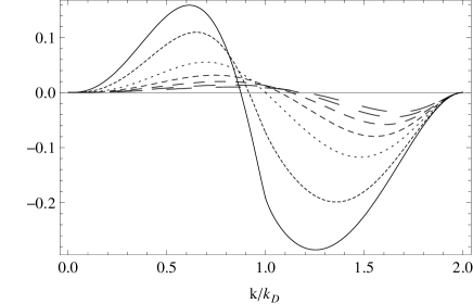
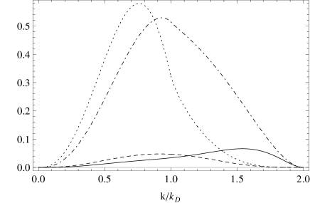
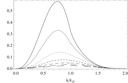
Figure 1: Non-helical (helical) contribution to $k^{3}\big{|}\rho(k)\big{|}^{2}$ in units of $\langle B^{2}\rangle^{2}/(4\pi)^{4}$ ($\langle\mathcal{B}^{2}\rangle^{2}/(4\pi)^{4}$) versus $k/k_{D}$ is plotted in the upper left (bottom left) panel. The total contribution is displayed in the bottom right panel for $\langle B^{2}\rangle^{2}=\langle\mathcal{B}^{2}\rangle^{2}$ and $n_{B}=n_{H}$. The different lines are for $n_{B}$ ($n_{H}$) = -3/2, -1, 0, 1, 2, 3, 4 ranging from the solid to the longest dashed. The panel in the upper right display the comparison between the non-helical case and the maximal helical case for $n_{B,\,H}=1$ (solid vs dashed) and $n_{B,\,H}=-3/2$ (dot-dashed vs dotted).

In this section we will describe the relevant terms of the scalar sector. The two-point correlation function of the energy density can be written in the Fourier space as:

$$\langle\rho(\mathbf{k})\rho^{*}(\mathbf{h})\rangle\equiv \,(2\pi)^{3}\delta^{(3)}(\mathbf{k}-\mathbf{h})\bigl{|}\rho(k)\bigr{|}^{2}\,,$$

$$= \,\delta_{ab}\delta_{cd}\langle\tau_{ab}(\mathbf{k})\tau^{*}_{cd}(\mathbf{h})\rangle\,.$$ (21)

Only the first two terms from Eq. (19), and their permutations, will contribute to this term and the energy density spectrum is therefore:

$$\bigl{|}\rho(k)\bigr{|}^{2} \equiv\bigl{|}\rho_{B}(k)\bigr{|}^{2}-2\bigl{|}\rho_{H}(k)\bigr{|}^{2}$$

$$=\int_{\Omega}\frac{d^{3}p}{(4\pi)^{5}}\Bigl{[}P_{B}(p)P_{B}(|\mathbf{k}-\mathbf{p}|)(1+\mu^{2})$$

$$\quad\quad\quad\quad\quad\quad-2P_{H}(p)P_{H}(|\mathbf{k}-\mathbf{p}|)\mu\Bigr{]}\,,$$ (22)

where $\mu\equiv\hat{p}\cdot\widehat{(\mathbf{k}-\mathbf{p})}=\frac{k\gamma-p}{\sqrt{k^{2}-2kp\gamma+p^{2}}}$ and $\gamma\equiv\hat{k}\cdot\hat{p}$.

For $k\ll k_{D}$ and $n_{B,\,H}>-3/2$ the energy density spectrum is:

$$\bigl{|}\rho(k)\bigr{|}^{2}\simeq\, \frac{A_{B}^{2}\,k_{D}^{2n_{B}+3}}{128\pi^{4}k_{*}^{2n_{B}}(2n_{B}+3)}$$

$$+\frac{A_{H}^{2}\,k_{D}^{2n_{H}+3}}{128\pi^{4}k_{*}^{2n_{H}}(2n_{H}+3)}\,.$$ (23)

For $n_{B,\,H}=-3/2$ we have a removable parametric divergence which is replaced by a logarithmic divergence in $k$, see the exact results in Appendix II.

See the panels in the left in Fig. 1 for the shape of $\bigl{|}\rho_{B}(k)\bigr{|}^{2}$ and $-2\bigl{|}\rho_{H}(k)\bigr{|}^{2}$ for different spectral indices. See the panel in the bottom right of Fig. 1 for the total contribution $\bigl{|}\rho(k)\bigr{|}^{2}$ in the maximal helical case, $A_{B}=A_{H}$, and $n_{B}=n_{H}$. The panel in the upper right of Fig. 1 displays the comparison of $\bigl{|}\rho(k)\bigr{|}^{2}$ in the non-helical case, $A_{H}=0$, and in the maximal helical case.

III.2 The scalar part of the Lorentz force

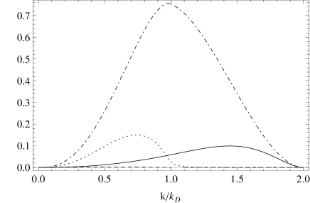
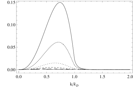
Figure 2: Non-helical (helical) contribution to $k^{3}\big{|}L(k)\big{|}^{2}$ in units of $\langle B^{2}\rangle^{2}/(4\pi)^{4}$ ($\langle\mathcal{B}^{2}\rangle^{2}/(4\pi)^{4}$) versus $k/k_{D}$ is plotted in the upper left (bottom left) panel. The different lines are for $n_{B}$ ($n_{H}$) = -3/2, -1, 0, 1, 2, 3, 4 ranging from the solid to the longest dashed. The panel in the upper right display the comparison between the non-helical case and the maximal helical case for $n_{B,\,H}=1$ (solid vs dashed) and $n_{B,\,H}=-3/2$ (dot-dashed vs dotted). The total contribution is displayed in the panel in the bottom right for $\langle B^{2}\rangle^{2}=\langle\mathcal{B}^{2}\rangle^{2}$ and $n_{B}=n_{H}$.

In order to compute the scalar contribution of a stochastic background of PMF to the cosmological perturbations, the convolution for the scalar part of the Lorentz force power spectrum is also necessary. In the MHD approximation, the Lorentz force is:

$$L(\mathbf{x})=-\frac{1}{4\pi}\Bigl{[}\mathbf{B}(\mathbf{x})\times\bigl{(}\nabla\times\mathbf{B}(\mathbf{x})\bigr{)}\Bigr{]}\,,$$ (24)

and so the two-point correlation function in Fourier space is:

$$\langle L(\mathbf{k})L^{*}(\mathbf{h})\rangle\equiv \,(2\pi)^{3}\delta^{(3)}(\mathbf{k}-\mathbf{h})\big{|}L(k)\big{|}^{2}$$

$$= \,\hat{k}_{a}\hat{k}_{b}\hat{k}_{c}\hat{k}_{d}\langle\tau_{ab}(\mathbf{k})\tau^{*}_{cd}(\mathbf{h})\rangle\,.$$ (25)

The spectrum of the Lorentz force is:

$$\big{|}L(k)\big{|}^{2} \equiv\big{|}L_{B}(k)\big{|}^{2}+\big{|}L_{H}(k)\big{|}^{2}$$

$$=\int_{\Omega}\frac{d^{3}p}{(4\,\pi)^{5}}\Bigl{[}P_{B}(p)P_{B}(|\mathbf{k}-\mathbf{p}|)\bigl{(}1+\mu^{2}+4\gamma^{2}\beta^{2}-4\gamma\beta\mu\bigr{)}+\,P_{H}(p)P_{H}(|\mathbf{k}-\mathbf{p}|)\bigl{(}2\mu-4\gamma\beta\bigr{)}\Bigr{]}\,,$$ (26)

where $\beta\equiv\hat{k}\cdot\widehat{(\mathbf{k}-\mathbf{p})}=\frac{k-p\gamma}{\sqrt{k^{2}-2kp\gamma+p^{2}}}$.

Also in this case the spectrum in the infrared limit, for $k\ll k_{D}$ and $n_{B,\,H}>-3/2$, behaves as:

$$\big{|}L(k)\big{|}^{2}\simeq\, \frac{11A_{B}^{2}\,k_{D}^{2n_{B}+3}}{1920\pi^{4}k_{*}^{2n_{B}}(2n_{B}+3)}$$

$$-\frac{A_{H}^{2}\,k_{D}^{2n_{H}+3}}{384\pi^{4}k_{*}^{2n_{H}}(2n_{H}+3)}\,.$$ (27)

See the panels on the left in Fig. 2 for the shape of $\bigl{|}L_{B}(k)\bigr{|}^{2}$ and $\bigl{|}L_{H}(k)\bigr{|}^{2}$ for different spectral indices. See the panel in the bottom right of Fig. 2 for the total contribution $\bigl{|}L(k)\bigr{|}^{2}$ in the maximal helical case, $A_{B}=A_{H}$, and $n_{B}=n_{H}$. Note from the panel in the upper right of Fig. 2 how the Lorentz force is decreased in the maximal helical case. The expression for the density-Lorentz force cross correlation shawlewis ; PF , including the helicity contribution, looks:

$$\langle\rho(k)L^{*}(k)\rangle=\int_{\Omega}\frac{d^{3}p}{(4\,\pi)^{5}}\left[P_{B}(p)P_{B}(|\mathbf{k}-\mathbf{p}|)\bigl{(}1-\mu^{2}-2\gamma^{2}-2\beta^{2}-2\gamma\beta\mu\bigr{)}-\,P_{H}(p)P_{H}(|\mathbf{k}-\mathbf{p}|)\left(\frac{2}{3}\mu-2\gamma\beta\right)\right]\,.$$ (28)

III.3 The scalar part of the anisotropic stress

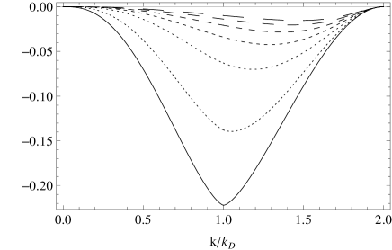
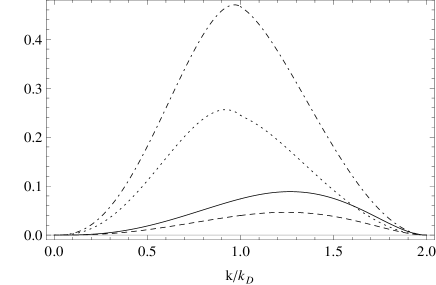
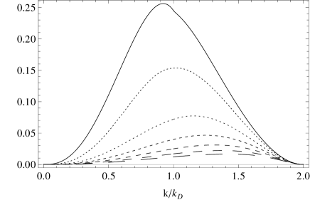
Figure 3: Non-helical (helical) contribution to $k^{3}\big{|}\sigma(k)\big{|}^{2}$ in units of $\langle B^{2}\rangle^{2}/(4\pi)^{4}$ ($\langle\mathcal{B}^{2}\rangle^{2}/(4\pi)^{4}$) versus $k/k_{D}$ is plotted in the upper left (bottom left) panel. The different lines are for $n_{B}$ ($n_{H}$) = -3/2, -1, 0, 1, 2, 3, 4 ranging from the solid to the longest dashed. The panel in the upper right display the comparison between the non-helical case and the maximal helical case for $n_{B,\,H}=1$ (solid vs dashed) and $n_{B,\,H}=-3/2$ (dot-dashed vs dotted). The total contribution is displayed in the bottom right panel for $\langle B^{2}\rangle^{2}=\langle\mathcal{B}^{2}\rangle^{2}$ and $n_{B}=n_{H}$.

For completeness we also write the scalar part of the anisotropic stress in function of the shear stress like Ma :

$$\sigma\equiv-\Bigl{(}\widehat{k}_{i}\widehat{k}_{j}-\frac{1}{3}\delta_{ij}\Bigr{)}\Sigma_{ij}\,,$$ (29)

where the stress shear is defined in our convention by:

$$\Sigma_{ij}=\tau_{ij}-\frac{1}{3}\delta_{ij}\tau_{ll}\,.$$ (30)

We are interested in the power spectrum of this quantity that is derived from the two-point correlator function as:

$$\langle\Pi^{(S)}_{ij}(\mathbf{k})\Pi^{(S)*}_{lm}(\mathbf{h})\rangle\equiv(2\pi)^{3}\delta^{(3)}(\mathbf{k}-\mathbf{h})\big{|}\sigma(k)\big{|}^{2}\,.$$ (31)

After a little algebra the spectrum reads:

$$\big{|}\sigma(k)\big{|}^{2} \equiv\big{|}\sigma_{B}(k)\big{|}^{2}+\big{|}\sigma_{H}(k)\big{|}^{2}$$

$$=\int_{\Omega}\frac{d^{3}p}{(4\pi)^{5}}\left\{P_{B}(p)P_{B}(|\mathbf{k}-\mathbf{p}|)\left[\frac{4}{9}(4+\mu^{2}-3\gamma^{2}-3\beta^{2}+9\gamma^{2}\beta^{2}-6\gamma\beta\mu)\right]+P_{H}(p)P_{H}(|\mathbf{k}-\mathbf{p}|)\left(\frac{16}{9}\mu-\frac{8}{3}\gamma\beta\right)\right\}\,.$$ (32)

See the panels on the right in Fig. 3 for the shape of $\bigl{|}\sigma_{B}(k)\bigr{|}^{2}$ and $\bigl{|}\sigma_{H}(k)\bigr{|}^{2}$ for different spectral indices. See the panel in the bottom right of Fig. 3 for the total contribution $\bigl{|}\sigma(k)\bigr{|}^{2}$ in the maximal helical case, $A_{B}=A_{H}$, and $n_{B}=n_{H}$.

IV The vector contribution

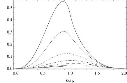
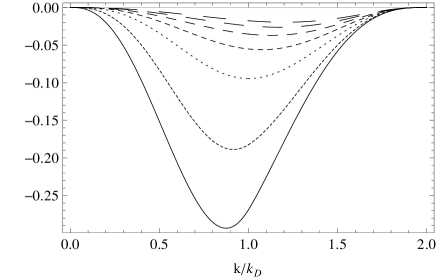
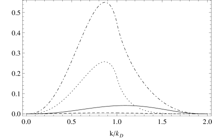
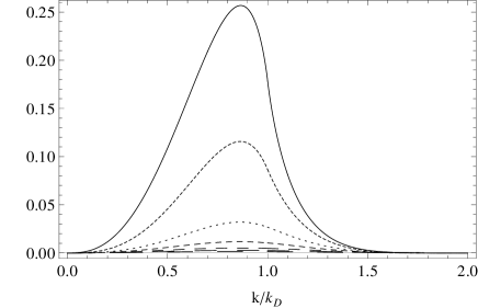
Figure 4: Non-helical (helical) contribution to $k^{3}\big{|}\Pi^{(V)}(k)\big{|}^{2}$ in units of $\langle B^{2}\rangle^{2}/(4\pi)^{4}$ ($\langle\mathcal{B}^{2}\rangle^{2}/(4\pi)^{4}$) versus $k/k_{D}$ is plotted in the upper left (bottom left) panel. The different lines are for $n_{B}$ ($n_{H}$) = -3/2, -1, 0, 1, 2, 3, 4 ranging from the solid to the longest dashed. The panel in the upper right display the comparison between the non-helical case and the maximal helical case for $n_{B,\,H}=1$ (solid vs dashed) and $n_{B,\,H}=-3/2$ (dot-dashed vs dotted). The total contribution is displayed in the bottom left panel for $\langle B^{2}\rangle^{2}=\langle\mathcal{B}^{2}\rangle^{2}$ and $n_{B}=n_{H}$.

In the standard $\Lambda$CDM model vector modes decay with the expansion of the Universe and have no observational signature at any significant level. However the associated temperature fluctuations, once generated, do not decay but in this case they have to be sourced by some shear, lewis:vector .

PMF carrying vector anisotropic stress generate a fully magnetized vector mode that is the dominant PMF compensated contribution to the CMB angular power spectra on small angular scales. On these scales the primary CMB is suppressed by Silk damping therefore magnetic vector mode dominates over CMB angular power spectrum as shown in PF_WMAP7SPT . The vector contribution to $\tau_{ab}$ is given by:

$$\Pi_{i}^{(V)}\equiv\hat{k}_{a}P_{ib}(k)\tau_{ab}\,.$$ (33)

We introduce the two-point correlation function for the vector source in the Fourier space, which can be parametrized as:

$$\langle\Pi^{(V)}_{i}(\mathbf{k})\Pi^{(V)*}_{j}(\mathbf{h})\rangle\equiv\frac{(2\pi)^{3}}{2}\delta^{(3)}(\mathbf{k}-\mathbf{h})\times$$

$$\qquad\qquad\times\Bigl{[}P_{ij}(k)\big{|}\Pi^{(V)}(k)\big{|}^{2}+\imath\epsilon_{ijl}\hat{k}_{l}X^{(V)}(k)\Bigr{]}\,.$$ (34)

Differently from the scalar case, the two-point correlation function for the vector source include an antisymmetric component. It is easy to separate the symmetric and the antisymmetric parts of the source spectra:

$$(2\pi)^{3}\delta^{(3)}(\mathbf{k}-\mathbf{h})\big{|}\Pi^{(V)}(k)\big{|}^{2}\equiv \,\frac{1}{2}\Bigl{[}P_{ai}(k)\hat{k}_{b}P_{ci}(h)\hat{h}_{d}+P_{bi}(k)\hat{k}_{a}P_{di}(h)\hat{h}_{c}\Bigr{]}\langle\tau_{ab}(\mathbf{k})\tau^{*}_{cd}(\mathbf{h})\rangle\,,$$ (35)

$$(2\pi)^{3}\delta^{(3)}(\mathbf{k}-\mathbf{h})X^{(V)}(k)\equiv -\frac{\imath}{2}\hat{k}_{i}\Bigl{[}\epsilon_{bdi}\hat{k}_{a}\hat{h}_{c}+\epsilon_{aci}\hat{k}_{b}\hat{h}_{d}\Bigr{]}\langle\tau_{ab}(\mathbf{k})\tau^{*}_{cd}(\mathbf{h})\rangle\,.$$ (36)

We obtain:

$$\big{|}\Pi^{(V)}(k)\big{|}^{2} \equiv\big{|}\Pi^{(V)}_{B}(k)\big{|}^{2}-\big{|}\Pi^{(V)}_{H}(k)\big{|}^{2}$$

$$=2\int_{\Omega}\frac{d^{3}p}{(4\pi)^{5}}\Bigl{\{}P_{B}(p)P_{B}(|\mathbf{k}-\mathbf{p}|)\bigl{[}(1+\beta^{2})(1-\gamma^{2})+\gamma\beta(\mu-\gamma\beta)\bigr{]}-P_{H}(p)P_{H}(|\mathbf{k}-\mathbf{p}|)(\gamma\beta-\mu)\Bigr{\}}\,,$$ (37)

$$X^{(V)}(k) =\int_{\Omega}\frac{d^{3}p}{(4\pi)^{5}}\biggl{\{}P_{B}(p)P_{H}(|\mathbf{k}-\mathbf{p}|)\bigl{[}\beta(1-\gamma^{2})-(\gamma\beta-\mu)\gamma\bigr{]}+P_{H}(p)P_{B}(|\mathbf{k}-\mathbf{p}|)\bigl{[}\gamma(1-\beta^{2})-(\gamma\beta-\mu)\beta\bigr{]}\biggr{\}}\,.$$ (38)

The behaviour of $\big{|}\Pi^{(V)}(k)\big{|}^{2}$ for $k\ll k_{D}$ and $n_{B,\,H}>-3/2$ has a white noise behaviour:

$$\big{|}\Pi^{(V)}(k)\big{|}^{2}\simeq\, \frac{7A_{B}^{2}\,k_{D}^{2n_{B}+3}}{960\pi^{4}k_{*}^{2n_{B}}(2n_{B}+3)}$$

$$-\frac{A_{H}^{2}\,k_{D}^{2n_{H}+3}}{192\pi^{4}k_{*}^{2n_{H}}(2n_{H}+3)}\,.$$ (39)

with a logarithmic divergence at $n_{B,\,H}=-3/2$. The antisymmetric spectrum has a different slope and is linear in $k$ for large wavelengths $k\ll k_{D}$ and for $n_{B}+n_{H}>-2$:

$$X^{(V)}(k)\simeq\frac{A_{B}\,A_{H}\,k_{D}^{n_{B}+n_{H}+2}}{960\pi^{4}k_{*}^{n_{B}+n_{H}}(n_{B}+n_{H}+2)}k\,.$$ (40)

The numerical coefficients obtained with semi-analytical approximation of the angular integral for the vector spectra in Kahniashvili:2005xe need to be multiplied, in our conventions, to 14/15 for $|\Pi^{(V)}_{B}(k)\big{|}^{2}$, as pointed in PFP ; the numerical coefficient for $|\Pi^{(V)}_{H}(k)\big{|}^{2}$ is in agreement with Ref. Kahniashvili:2005xe . A larger numerical coefficient $1/5$ is needed for previous calculations which neglected the angular integration to match our result $X^{(V)}(k)$ Kahniashvili:2005xe .
The pole at $n_{B}+n_{H}=-2$ in Eq. (IV) is removable and we find for this choice of parameters:

$$X^{(V)}(k)\simeq-\frac{A_{B}\,A_{H}\,k_{*}^{2}}{5760\pi^{4}}k\log(k/k_{D})\,.$$ (41)

For $n_{B,\,H}=-3/2$ we obtain:

$$X^{(V)}(k)\simeq\frac{A_{B}\,A_{H}\,k_{*}^{3}}{1536\pi^{3}}\,.$$ (42)

Note that the convolution integral for $X^{(V)}(k)$ in Eq. (38) in the maximal helical case does not require infrared cut-offs for $n_{B}+n_{H}>-3$.

As for the scalar parts, Fig. 4 displays on the left column the non-helical and helical part of the vector anisotropies $\big{|}\Pi^{(V)}(k)\big{|}^{2}$ when the spectral index is varied. The panel in the upper right displays the comparison between the non-helical and the helical case for the symmetric vector spectrum. The panel in the bottom right displays the total $\big{|}\Pi^{(V)}(k)\big{|}^{2}$.

V The tensor contribution

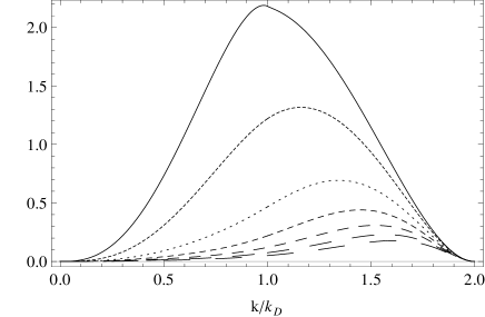
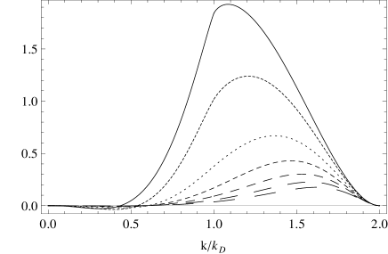
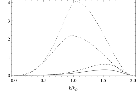
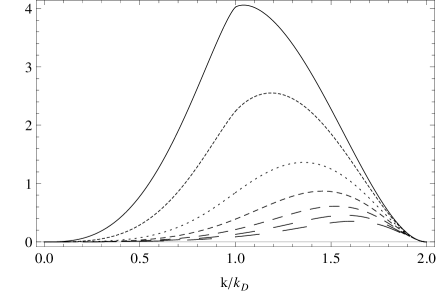
Figure 5: Non-helical (helical) contribution to $k^{3}\big{|}\Pi^{(T)}(k)\big{|}^{2}$ in units of $\langle B^{2}\rangle^{2}/(4\pi)^{4}$ ($\langle\mathcal{B}^{2}\rangle^{2}/(4\pi)^{4}$) versus $k/k_{D}$ is plotted in the upper left (bottom left) panel. The different lines are for $n_{B}$ ($n_{H}$) = -3/2, -1, 0, 1, 2, 3, 4 ranging from the solid to the longest dashed. The panel in the upper right display the comparison between the non-helical case and the maximal helical case for $n_{B,\,H}=1$ (solid vs dashed) and $n_{B,\,H}=-3/2$ (dot-dashed vs dotted). The total contribution is displayed in the bottom right panel for $\langle B^{2}\rangle^{2}=\langle\mathcal{B}^{2}\rangle^{2}$ and $n_{B}=n_{H}$.

PMF source tensor modes from tensor anisotropic pressure. The tensor part of the magnetic field EMT is given by:

$$\Pi_{ij}^{(T)}(\mathbf{k})\equiv\mathcal{P}_{ijab}(k)\tau_{ab}(\mathbf{k})\,,$$ (43)

with the tensor projector $\mathcal{P}_{ijab}$ as:

$$\mathcal{P}_{ijab}(k)=P_{ia}(k)P_{jb}(k)-\frac{1}{2}P_{ij}(k)P_{ab}(k)\,.$$ (44)

We define the tensor projector to apply on $\langle\tau_{ab}(\mathbf{k})\tau^{*}_{cd}(\mathbf{h})\rangle$ as:

$$\mathcal{P}^{abcd}_{ijlm}(k,h)\equiv\mathcal{P}_{ijab}(k)\mathcal{P}_{lmcd}(h)\,.$$ (45)

As for the vector case, we introduce the two-point correlation function for the tensor source as:

$$\langle\Pi^{(T)}_{ij}(\mathbf{k})\Pi^{(T)*}_{lm}(\mathbf{h})\rangle\equiv\frac{(2\pi)^{3}}{4}\delta^{(3)}(\mathbf{k}-\mathbf{h})\times$$ (46)

$$\qquad\qquad\times\Bigl{[}\mathcal{M}_{ijlm}\big{|}\Pi^{(T)}(k)\big{|}^{2}+\imath\mathcal{A}_{ijlm}X^{(T)}(k)\Bigr{]}\,,$$

where the tensors $\mathcal{M}_{ijlm}$ and $\mathcal{A}_{ijlm}$ are given by:

$$\mathcal{M}_{ijlm}\equiv P_{il} P_{jm}+P_{im}P_{jl}-P_{ij}P_{lm}\,,$$ (47)

$$\mathcal{A}_{ijlm}\equiv\frac{\hat{k}_{t}}{2}\bigl{(} P_{il}\epsilon_{jmt}+P_{im}\epsilon_{jlt}$$

$$+P_{jl}\epsilon_{imt}+P_{jm}\epsilon_{ilt}\bigr{)}\,.$$ (48)

Both $\mathcal{M}_{ijlm}$ and $\mathcal{A}_{ijlm}$ are symmetric under permutations $(i\leftrightarrow j)$ and $(l\leftrightarrow m)$; $\mathcal{M}_{ijlm}$ is also symmetric under the exchange of $(ij)\leftrightarrow(lm)$, whereas $\mathcal{A}_{ijlm}$ is antisymmetric under this permutation. We can summarize the previous rules with the properties:

$$\mathcal{M}_{ijij}=4\,,\quad\mathcal{M}_{iilm}=\mathcal{M}_{ijll}=0\,,$$ (49)

$$\mathcal{A}_{ijij}=\mathcal{A}_{iilm}=\mathcal{A}_{ijll}=0\,,$$ (50)

$$|\mathcal{M}|^{2}=|\mathcal{A}|^{2}=8\,,$$ (51)

$$\mathcal{M}_{ijlm}\mathcal{A}_{ijlm}=0\,.$$ (52)

The source terms for the tensor parts are:

$$(2\pi)^{3}\delta^{(3)}(\mathbf{k}-\mathbf{h})\big{|}\Pi^{(T)}(k)\big{|}^{2} \equiv\frac{1}{2}\mathcal{M}_{abcd}\langle\tau_{ab}(\mathbf{k})\tau^{*}_{cd}(\mathbf{h})\rangle\,,$$ (53)

$$(2\pi)^{3}\delta^{(3)}(\mathbf{k}-\mathbf{h})X^{(T)}(k) \equiv-\frac{\imath}{2}\mathcal{A}_{abcd}\langle\tau_{ab}(\mathbf{k})\tau^{*}_{cd}(\mathbf{h})\rangle\,.$$ (54)

We find for the source spectra:

$$\big{|}\Pi^{(T)}(k)\big{|}^{2} \equiv\big{|}\Pi^{(T)}_{B}(k)\big{|}^{2}+4\big{|}\Pi^{(T)}_{H}(k)\big{|}^{2}=2\int_{\Omega}\frac{d^{3}p}{(4\pi)^{5}}\Bigl{[}P_{B}(p)P_{B}(|\mathbf{k}-\mathbf{p}|)(1+\gamma^{2})(1+\beta^{2})+4P_{H}(p)P_{H}(|\mathbf{k}-\mathbf{p}|)\gamma\beta\Bigr{]}\,,$$ (55)

$$X^{(T)}(k) =4\int_{\Omega}\frac{d^{3}p}{(4\pi)^{5}}\biggl{[}P_{B}(p)P_{H}(|\mathbf{k}-\mathbf{p}|)(1+\gamma^{2})\beta+P_{H}(p)P_{B}(|\mathbf{k}-\mathbf{p}|)\gamma(1+\beta^{2})\biggr{]}\,.$$ (56)

As for the vector sector we obtain an antisymmetric power spectrum. The tensor anisotropic stress spectra is similar to the vector ones for $n_{B,\,H}>-3/2$:

$$\big{|}\Pi^{(T)}(k)\big{|}^{2}\simeq\, \frac{7A_{B}^{2}\,k_{D}^{2n_{B}+3}}{480\pi^{4}k_{*}^{2n_{B}}(2n_{B}+3)}$$

$$-\frac{A_{H}^{2}\,k_{D}^{2n_{H}+3}}{96\pi^{4}k_{*}^{2n_{H}}(2n_{H}+3)}\,,$$

$$X^{(T)}(k)\simeq\, \frac{A_{B}\,A_{H}\,k_{D}^{n_{B}+n_{H}+2}}{480\pi^{4}k_{*}^{n_{B}+n_{H}}(n_{B}+n_{H}+2)}k\,.$$ (57)

In this case the numerical coefficients obtained with semi-analytical approch in CDK differ from the exact result of a factor 28/15 for $|\Pi^{(T)}_{B}(k)\big{|}^{2}$ and 1/2 for $|\Pi^{(T)}_{H}(k)\big{|}^{2}$. Moreover the relation between the vector and tensor anisotropic stresses is different: we found that for the white noise spectra is still valid the relation $|\Pi^{(T)}(k)\big{|}^{2}\simeq 2|\Pi^{(V)}(k)\big{|}^{2}$ taking into account these new contributions to the even correlators. $X^{(T)}(k)$ is different by a factor 1/5.

The pole at $n_{B}+n_{H}=-2$ is removable and we find for the antisymmetric part:

$$X^{(T)}(k)\simeq-\frac{A_{B}\,A_{H}\,k_{*}^{2}}{120\pi^{4}}k\log(k/k_{D})\,.$$ (58)

For $n_{B,\,H}=-3/2$ we obtain:

$$X^{(T)}(k)\simeq\frac{7A_{B}\,A_{H}\,k_{*}^{3}}{768\pi^{3}}\,.$$ (59)

Note that the convolution integral for $X^{(T)}(k)$ in Eq. (38) in the maximal helical case does not require infrared cut-offs for $n_{B}+n_{H}>-3$.

Fig. 5 displays on the left column the non-helical, $\big{|}\Pi_{B}^{(T)}(k)\big{|}^{2}$, and helical part, $4\big{|}\Pi_{H}^{(T)}(k)\big{|}^{2}$, of the tensor anisotropies $\big{|}\Pi^{(T)}(k)\big{|}^{2}$ when the spectral index is varied. The panel in the bottom right displays the total $\big{|}\Pi^{(T)}(k)\big{|}^{2}$ for the maximal helical case when $n_{B}=n_{H}$ is varying.

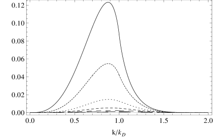
Figure 6: Comparison of antisymmetric correlators in units of $\langle B^{2}\rangle\langle\mathcal{B}^{2}\rangle/(4\pi)^{4}$, the different lines are for $n_{B}=n_{H}=-3/2,-1,0,1,2,3,4$ ranging from the solid to the longest dashed. The vector one, $k^{3}X^{(V)}(k)$, in the upper panel and the tensor one, $k^{3}X^{(T)}(k)$, in the bottom panel.

The left panel of Fig. 6 displays the antisymmetric $X^{(V)}(k)$ when varying $n_{B}=n_{H}$. The right panel correspond to the tensor one $X^{(T)}(k)$.

VI CMB anisotropies

We now investigate how helicity changes the PMF contribution to CMB power spectrum anisotropies in temperature and polarization. We included the helical contribution of the PMF EMT in our modified version of the public Einstein-Boltzmann code CAMB CAMB which was used based on the already existent one from FPP ; PFP to derive the angular power spectra.

VI.1 The scalar contribution to CMB anisotropies

The scalar contribution is the sum of the helical and non-helical terms in the density, Lorentz and corresponding cross-correlations.

In Fig. 7 we show the contributions to the total CMB temperature angular power spectra from the scalar pure magnetic mode for different fixed spectral indices and its comparison with the adiabatic mode.

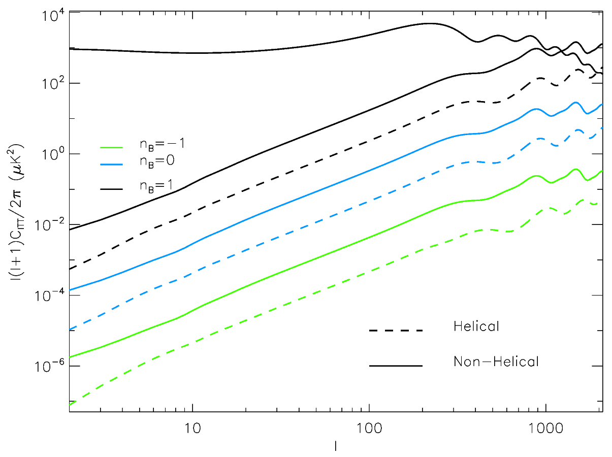
Figure 7: We show the scalar power spectrum with the cross-correlation between $\rho_{B}$ and $L_{B}$. The solid line is the adiabatic scalar contribution in comparison with the scalar contributions of a stochastic background of PMF for $\sqrt{\langle B^{2}_{\lambda}\rangle}=3.5\,nG$.

VI.2 The vector contribution to CMB anisotropies

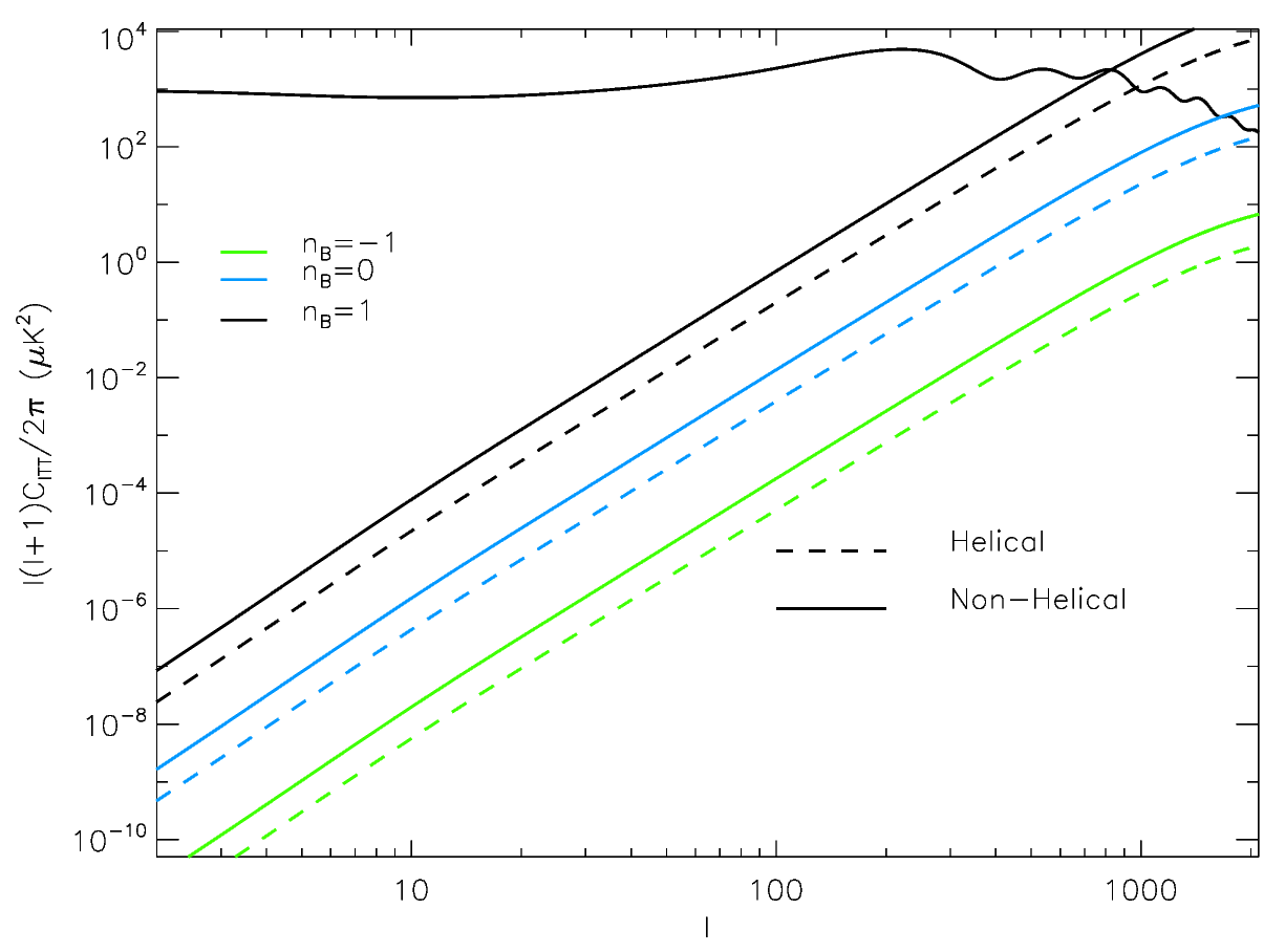
Figure 8: CMB anisotropies angular power spectrum for temperature. The solid line is the adiabatic scalar contribution in comparison with the vector contributions of a stochastic background of PMF for $\sqrt{\langle B^{2}_{\lambda}\rangle}=3.5\ nG$.

To understand how the antisymmetric component of the vector source term in Eq. (38) afflict the CMB power spectrum anisotropies it is useful to rewrite the spectrum in a polarization orthonormal base that for the helical case will be:

$$\mathbf{e}^{\pm}(\mathbf{k})=-\frac{\imath}{\sqrt{2}}(\mathbf{e}^{+}\pm\imath\mathbf{e}^{-})\,,$$ (60)

with the following properties:

$$\mathbf{e}^{\pm}\cdot\mathbf{e}^{\mp}=-1\,,$$ (61)

$$\mathbf{e}^{\pm}\cdot\mathbf{e}^{\pm}=0\,,$$ (62)

$$\mathbf{e}^{\pm}(\mathbf{k})=\mathbf{e}^{\mp}(-\mathbf{k})\,.$$ (63)

With this choice we obtain the decomposition:

$$\Pi^{(V)}_{i}(\mathbf{k})=e_{i}^{+}\Pi^{+}_{V}(\mathbf{k})+e_{i}^{-}\Pi^{-}_{V}(\mathbf{k})$$ (64)

that allow us to rewrite (35) and (36) into:

$$(2\pi)^{3}\delta^{(3)}(\mathbf{k}-\mathbf{h})\big{|}\Pi^{(V)}_{B}(k)\big{|}^{2}=$$

$$\qquad\langle\Pi^{+}_{V}(\mathbf{k})\Pi^{+*}_{V}(\mathbf{-h})+\Pi^{-}_{V}(\mathbf{k})\Pi^{-*}_{V}(\mathbf{-h})\rangle\,,$$ (65)

$$(2\pi)^{3}\delta^{(3)}(\mathbf{k}-\mathbf{h})X^{(V)}(k)=$$

$$\qquad-\langle\Pi^{+}_{V}(\mathbf{k})\Pi^{+*}_{V}(\mathbf{-h})-\Pi^{-}_{V}(\mathbf{k})\Pi^{-*}_{V}(\mathbf{-h})\rangle\,.$$ (66)

In conclusion for the vector sector we will have two independent metric perturbation modes which are sourced by combinations of $\big{|}\Pi^{(V)}\big{|}^{2}$ and $X^{(V)}$:

$$\dot{h}^{\pm}_{V}+2\mathcal{H}h^{\pm}_{V}=-16\pi Ga^{2}\frac{\Pi_{\nu}^{(V)}+\Pi_{\gamma}^{(V)}+\Pi_{V}^{\pm}}{k}\,.$$ (67)

We note that the angular power spectrum peaks around $l\sim 2000$ according to PFP ; lewis . The peak is in the region where primary CMB is suppressed by Silk damping, therefore magnetized vector anisotropies are the dominant compensated contribution on small scales. The vector part of the Lorentz force induced on baryons modifies the baryon vector velocity equation:

$$\dot{v}_{b}+\mathcal{H}v_{b}=-\frac{\rho_{\gamma}}{\rho_{b}}\Bigl{[}\frac{4}{3}n_{e}a\sigma_{T}(v_{b}-v_{\gamma})-\frac{L^{V}}{\rho_{\gamma}}\Bigr{]}\,.$$ (68)

Considering Eq. (III.2) we will have a slightly deviation from the non-helical case. Fig. 8 shows the vector contribution to the $TT$ spectrum and its dependence from the spectral indices.

Due to the helical contribution the parity odd CMB power spectra are non-zero. In particular their presence is due to the antisymmetric source Eq. (38) which emphasizes the difference between the two polarizations $+$ and $-$. As shown in PVW these antisymmetric sources generate the parity odd spectra $C_{l}^{TB},\,C_{l}^{EB}$, since they are given by momentum integrals of $X^{(V)}(k)$:

$$C_{l}^{TB}=\frac{2}{\pi}\int_{0}^{\infty}k^{2}dk\,X^{(V)}(k)\Delta_{l}(k)B_{l}(k)\,,$$ (69)

$$C_{l}^{EB}=\frac{2}{\pi}\int_{0}^{\infty}k^{2}dk\,X^{(V)}(k)E_{l}(k)B_{l}(k)\,,$$ (70)

where $\Delta_{l}(k)$, $E_{l}(k)$ and $B_{l}(k)$ contain all the information about the CMB transfer functions.

From Fig. 9, we can see that the resulting $\ell(\ell+1)C_{l}^{TB}/(2\pi)$ is of the order of ${\cal O}(10^{-1})$ $\mu$K² for $n_{B}=n_{H}=0$ at $\ell\sim 10^{3}$ for the maximal helical case with $\sqrt{\langle B_{\lambda}^{2}\rangle}=3.5\ nG$. For comparison, the vector contribution $\ell(\ell+1)C_{l}^{TT}/(2\pi)$ to the temperature anisotropies for a non-helical stochastic background is larger than ${\cal O}(10^{2})$ $\mu$K² for $\sqrt{\langle B_{\lambda}^{2}\rangle}=3.5\ nG$ and $n_{B}=0$ and is roughly ${\cal O}(10^{2})$ $\mu$K² in the maximal helical case at $\ell=10^{3}$. These values need to be compared with a typical value for the $\Lambda$CDM best-fit model of the order of ${\cal O}(10^{3})$ $\mu$K² at $\ell=10^{3}$.

In a recent paper Kahniashvili:2014dfa , WMAP 9 yr $TB$ data have been used to constrain the helical odd-parity vector contribution of a stochastic background of primordial magnetic fields.
In Kahniashvili:2014dfa the basic assumptions in terms of simple power spectra for the non-helical and helical contributions with a sharp cut-off at $k=k_{D}$ are the same as in this paper, however, there is a strong difference in the treatment of the maximum helical condition. They use the integrated measure ${\cal H}$ in Eq. (II) and therefore allows the range $n_{H}>-2$ without the use of an integrated cut-off; this results in a bound of ${\cal H}<10\ nG^{2}\ Gpc$ as a 95% CL for $\sqrt{\langle B^{2}\rangle}=3\ nG$ and $n_{B}=n_{H}-1=-2.9$ from WMAP 9 yr $TB$ data.

We first show that the bound quoted in Kahniashvili et al. Kahniashvili:2014dfa is much larger than what admitted by the Schwarz’s inequality for amplitudes of the non-helical part constrained by current CMB data. We obtain the maximum value for $A_{H}^{\mathrm{m}ax}=A_{B}(k_{*}/k_{D})$ by imposing the inequality in Eq. (5) to be valid at all $k\leq k_{D}$ for $n_{B}=n_{H}-1=-2.9$. As a maximum value for ${\cal H}$, we therefore obtain for the same values of the two spectral indices:

$${\cal H}^{\mathrm{m}ax}=\frac{\langle B^{2}\rangle}{16\pi k_{D}}\,.$$ (71)

The bounds coming from Eq. (71) for a typical value of the damping scale according to Refs. Jedamzik:1996wp ; stochastic background , i.e. in the range of $10^{2}\ Mpc^{-1}$ is about seven orders of magnitude smaller than the 95% bound $10\ nG^{2}\ Gpc$. In order to respect the maximum helical condition imposed by Eq. (71) it would be necessary to consider a damping scale of the order of $k_{D}\sim 2\times 10^{-2}\ Gpc^{-1}$ which would suppress all the contributions of primordial magnetic fields apart from the very large angular scales, namely only the very first multipoles of the CMB anisotropy angular power spectra.

In addition, there are values of parameters which are excluded by considering ${\cal H}$ instead of ${\cal B}$ for which $C_{\ell}^{TB}$ could be larger. Our treatment allows to compute the parity-odd $X^{(V)}(k)$ for spectral indices $n_{B}\neq n_{H}$. In Fig. 10, $X^{(V)}(k)$ with $n_{B}=n_{H}-1=-2.9$ is compared with the two maximal helical cases $n_{B}=n_{H}=-2.9$ and $n_{B}=n_{H}=-1.9$. As expected, $X^{(V)}(k)$ for the $n_{B}=n_{H}-1=-2.9$ lies between the two maximal helical cases with $n_{B}=n_{H}=-2.9$ and $n_{B}=n_{H}=-1.9$. For the wavenumbers relevant for CMB anisotropies, i.e. $k\ll k_{D}$, the maximal helical nearly scale-invariant case with $n_{B}=n_{H}=-2.9$ is larger than the $n_{B}=n_{H}-1=-2.9$.

The results of this analysis show how the currently publicly available WMAP 9 yr $TB$ data are hardly sensitive to constrain the helical odd-parity vector contribution at values comparable with those obtained by the inequality in Eq. (5) for amplitudes of the non-helical part at the level of $nG$ and values of the spectral indices as $n_{B}=n_{H}-1=-2.9$ . Different considerations would hold for the tensor contribution.

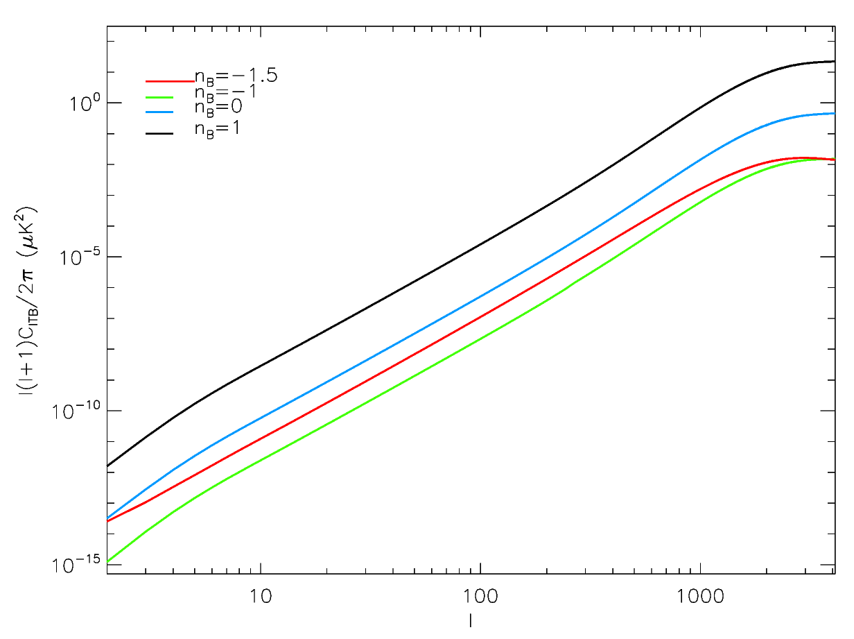
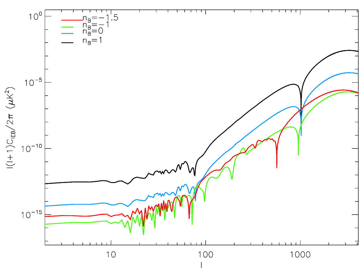
Figure 9: On the top panel we show the parity-odd vector power spectrum $TB$ and in the bottom panel the parity-odd correlator $EB$, with a magnetic field $\sqrt{\langle B^{2}_{\lambda}\rangle}=3.5\ nG$.

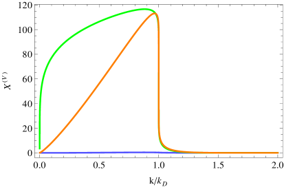
Figure 10: Comparison of $k^{3}X^{(V)}(k)$ (in units of $\langle B^{2}\rangle\langle\mathcal{B}^{2}\rangle/(4\pi)^{4}$), for $n_{B}=n_{H}=-1.9$ (blue line), $n_{B}=n_{H}-1=-2.9$ (orange line) and $n_{B}=n_{H}=-2.9$ (green line).

VI.3 The tensor contribution to CMB anisotropies

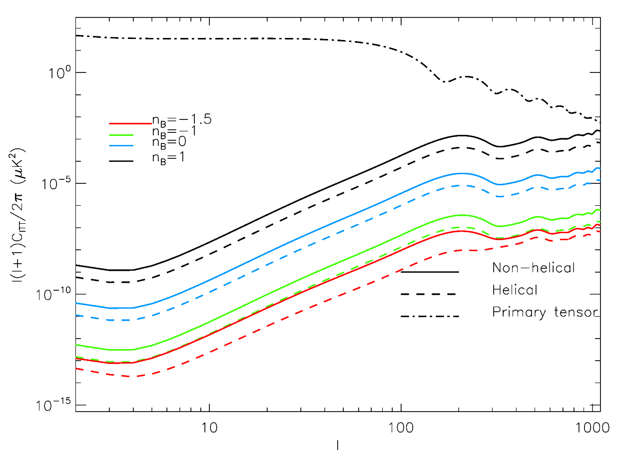
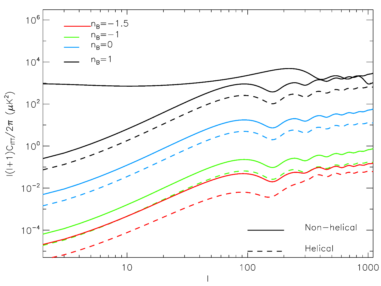
Figure 11: CMB anisotropies angular power spectrum for temperature. We include the tensor primary contribution from adiabatic inflation in comparison with the tensor contributions of a stochastic background of PMF for $\sqrt{\langle B^{2}_{\lambda}\rangle}=3.5\ nG$. In the top panel we show the compensated mode and in the bottom one the passive mode.

The evolution of tensor metric perturbations is described by Einstein equations where PMF contribution is again an additional source term, given by PMF stress tensor:

$$\ddot{h}_{ij}+2\mathcal{H}\dot{h}_{ij}+k^{2}h_{ij}=16\pi Ga^{2}\bigl{(}\rho_{\nu}\pi^{\nu}_{ij}+\Pi^{(T)}_{ij}\bigr{)}\,.$$ (72)

As in the vector case we can use a consistent tensor orthonormal polarization base to divide the metric solution respect to the two independent sources. Consider:

$$e_{ij}^{\pm}=-\sqrt{\frac{3}{8}}(\mathbf{e}_{1}\pm\imath\mathbf{e}_{2})_{i}\times(\mathbf{e}_{1}\pm\imath\mathbf{e}_{2})_{j}\,,$$ (73)

with the following properties:

$$e_{ij}^{\pm}e_{ij}^{\pm}=0\,,$$ (74)

$$e_{ij}^{\pm}e_{ij}^{\mp}=\frac{3}{2}\,,$$ (75)

$$(e_{ij}^{\pm})^{*}=e_{ij}^{\mp}\,.$$ (76)

In this basis the tensor part of the anisotropic stress is expressed as:

$$\Pi_{ij}^{(T)}(\mathbf{k})=e_{ij}^{+}\Pi^{+}_{T}(\mathbf{k})+e_{ij}^{-}\Pi^{-}_{T}(\mathbf{k})\,.$$ (77)

Now, we can rewrite the EMT source in terms of the component $\Pi^{\pm}_{T}$ and viceversa as:

$$(2\pi)^{3}\delta^{(3)}(\mathbf{k}-\mathbf{h})\big{|}\Pi^{(T)}_{B}(k)\big{|}^{2}=$$

$$\qquad\frac{3}{2}\langle\Pi^{-}_{T}(\mathbf{k})\Pi^{-\,*}_{T}(\mathbf{h})+\Pi^{+}_{T}(\mathbf{k})\Pi^{+\,*}_{T}(\mathbf{h})\rangle\,,$$ (78)

$$(2\pi)^{3}\delta^{(3)}(\mathbf{k}-\mathbf{h})X^{(T)}(k)=$$

$$\qquad-\frac{3}{2}\langle-\Pi^{-}_{T}(\mathbf{k})\Pi^{-\,*}_{T}(\mathbf{h})+\Pi^{+}_{T}(\mathbf{k})\Pi^{+\,*}_{T}(\mathbf{h})\rangle\,,$$ (79)

and so we can split the Eq. (72) in two polarization states $+$ and $-$, as we previously made for the vector case.

As for the vector case, tensor magnetic source spectrum has an helical contribution that gives non-vanishing odd CMB power spectra. In Figs. 11 and 12 are shown the angular power spectra of the temperature polarization CMB’s anisotropies due to the tensor modes for compensated and passive initial condition.

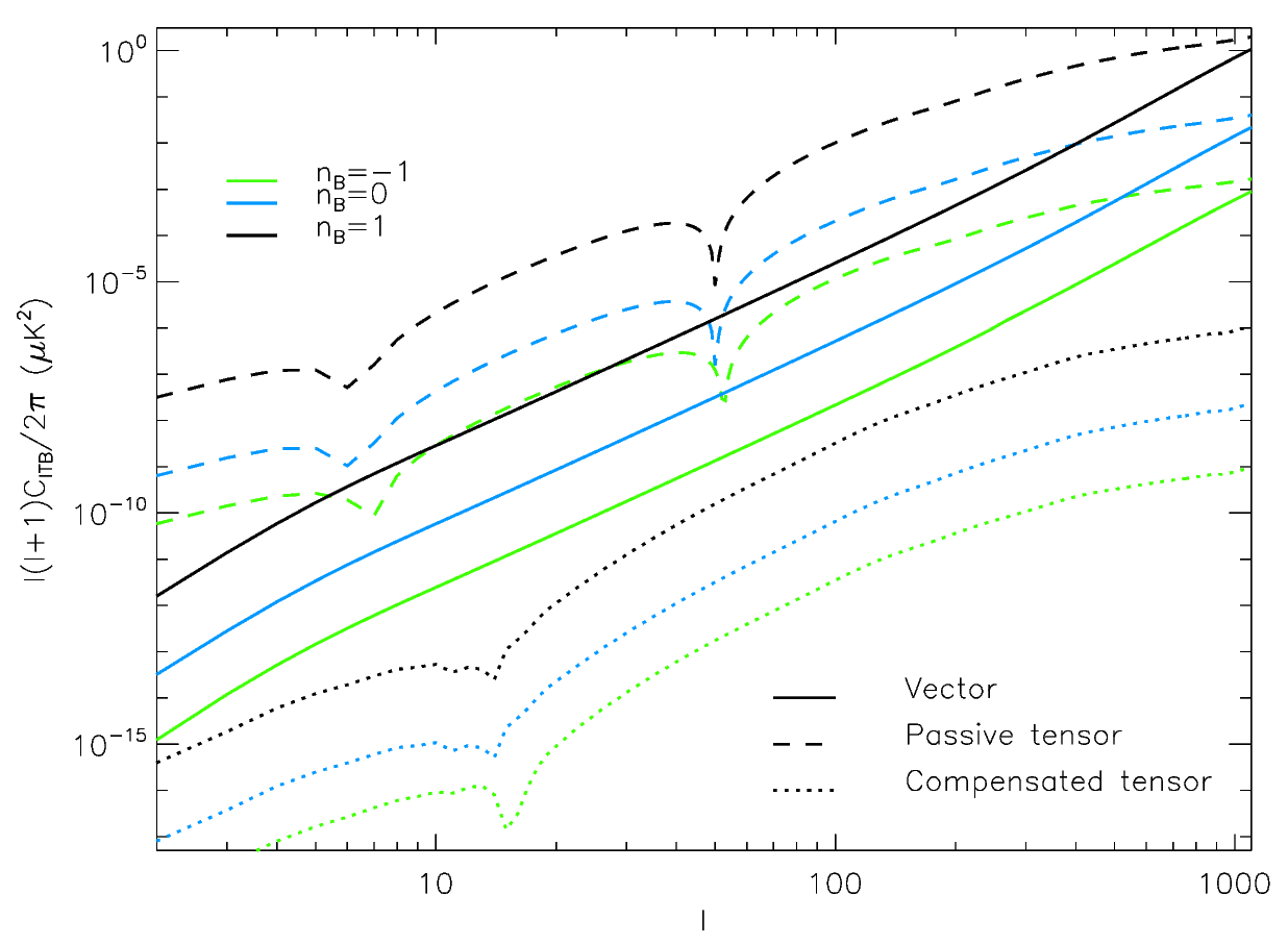
Figure 12: Comparison between the vector, compensated tensor and passive tensor $C_{l}^{TB}$ spectrum.

VII Conclusions

We have studied the helical contribution to the EMT of a stochastic primordial background of PMF extending the previous treatment in the non-helical case FPP ; PFP .

Under the assumption of a sharp cutoff for the damping scale, we gave the exact expressions of the Fourier convolutions of the EMT for the values of the selected spectral index $n_{H}$. The helical contribution to the EMT components is of a similar order of magnitude of the non-helical case. As for the non-helical case, the integration of the angular part leads to different numerical coefficient with respect to the previous results CDK ; Kahniashvili:2005xe .

We have then computed the CMB anisotropy power spectra in temperature and polarization of the stochastic background for $\ell<3000$. Such numerical computation for the power spectra to high $\ell$ allows the comparison of theoretical predictions with observations in the regime where the PMF contribution is higher.

There are two main effects when taking into account a possible helical contribution. The first effect is the modification of the parity even contribution to $C_{\ell}^{TT}\,,C_{\ell}^{EE}\,,C_{\ell}^{BB}\,,C_{\ell}^{TE}$. This contribution in the case of maximal helicity is negative for scalar, vector and tensor and decrease the $C_{\ell}$. Since the helical and non-helical parity-even contributions have a similar asymptotic dependence on $k$ for $k\ll k_{D}$, a maximal helical contribution is nearly degenerate to the non-helical one with smaller amplitude. The EMT Fourier spectra and the CMB predictions derived here are used in Ref. Adam:2015rua to derive the Planck 2015 constraints for the maximal helical case.

The second effect is the generation of the parity odd cross-correlation $C_{\ell}^{TB}$ and $C_{\ell}^{EB}$, which would otherwise vanish in absence of helicity. Current QUAD ; BICEP ; WMAP9 and future Planck data will be useful to help breaking this degeneracy.

Acknowledgements. We acknowledge discussions and suggestions by Chiara Caprini. We acknowledge support by PRIN MIUR 2009 grant n. 2009XZ54H2 and ASI through ASI/INAF Agreement I/072/09/0 for the Planck LFI Activity of Phase E2.

I Appendix

As for the non-helical EMT components studied in FPP ; PFP ; PF , our computations include a careful integration of the angular part, often neglected MKK ; KR ; CDK previous to Ref. FPP .

We use the convolutions for the PMF EMT spectra with the parametrization for the magnetic field PS given in Eqs. (6) and (7). Since $P_{B}(k)=0$ and $P_{H}(k)=0$ for $k>k_{D}$, two conditions need to be taken into account: $p<k_{D}$ and $\big{|}{\bf k}-{\bf p}\big{|}<k_{D}$.

The second condition introduces a $k$-dependence on the angular integration domain and the two allow the energy power spectrum to be non zero only for $0<k<2k_{D}$. Such conditions split the double integral (over $\gamma$ and over $p$) in three parts depending on the $\gamma$ and $p$ lower and upper limit of integration. A sketch of the integration is thus the following:

$$1) 0<k<k_{D}$$

$$\int_{0}^{k_{D}-k}dp\int_{-1}^{1}d\gamma\,\dots+\int_{1-k}^{1}dp\int_{\frac{k^{2}+p^{2}-k_{D}^{2}}{2kp}}^{1}d\gamma\,\dots\equiv\int_{0}^{k_{D}-k}dpI_{a}(p,k)+\int_{k_{D}-k}^{k_{D}}dpI_{S}(p,k)$$

$$2) k_{D}<k<2k_{D}$$ (80)

$$\int_{k-k_{D}}^{k_{D}}dp\int_{\frac{k^{2}+p^{2}-k_{D}^{2}}{2kp}}^{1}d\gamma\,\dots\equiv\int_{k-k_{D}}^{k_{D}}dpI_{c}(p,k)$$

Particular care must be used in the radial integrals. In particular, the presence of the term $|k-p|^{n+2}$ in both integrands, needs a further splitting of the integral domain for odd $n$:

$$\int_{0}^{(k_{D}-k)}dp\rightarrow\left\{\begin{array}[]{ll}k<k_{D}/2\left\{\begin{array}[]{ll}\int_{0}^{k}dp...&{\rm with}\quad p<k\\ \int_{k}^{(k_{D}-k)}dp...&{\rm with}\quad p>k\\ \end{array}\right.\\ k>k_{D}/2\quad\int_{0}^{(1-k)}dp...\quad{\rm with}\quad p<k\\ \end{array}\right.$$

$$\int_{(k_{D}-k)}^{1}dp\rightarrow\left\{\begin{array}[]{ll}k<k_{D}/2\quad\int_{(1-k)}^{1}dp...\qquad{\rm with}\quad p>k\\ k>k_{D}/2\left\{\begin{array}[]{ll}\int_{(k_{D}-k)}^{k}dp...&{\rm with}\quad p<k\\ \int_{k}^{1}dp...&{\rm with}\quad p>k\\ \end{array}\right.\end{array}\right.$$

$$\int_{k-k_{D}}^{1}dp\rightarrow\left\{\begin{array}[]{ll}1<k<2\quad\int_{k-k_{D}}^{1}dp...\quad{\rm with}\quad p<k\\ \end{array}\right.$$

II Appendix

Following the scheme in Appendix I we can now perform the integration over $\mathbf{p}$ for the selected correlators in Eqs. (III.1), (IV), (38), (55), (56), (III.2) and (III.3).

Correlators for scalar perturbations
Our exact results for $|\rho_{B}(k)|^{2}$ and $|\rho_{H}(k)|^{2}$ are given for particular values of $n_{B}$ and $n_{H}$.

II.0.1 $n_{B},\,n_{H}=4$

$$|\rho_{B}(k)|^{2}=\frac{A_{B}^{2}\,k_{D}^{11}}{512\,\pi^{4}\,k_{*}^{8}}\biggl{[}\frac{4}{11}-\tilde{k}+\frac{4\tilde{k}^{2}}{3}-\tilde{k}^{3}+\frac{8\tilde{k}^{4}}{21}-\frac{\tilde{k}^{5}}{24}-\frac{\tilde{k}^{7}}{192}+\frac{\tilde{k}^{11}}{9856}\biggl{]}\,,$$

$$|\rho_{H}(k)|^{2}=\frac{A_{H}^{2}\,k_{D}^{11}}{512\,\pi^{4}\,k_{*}^{8}}\left\{\begin{array}[]{ll}-\frac{2}{11}+\frac{\tilde{k}}{2}-\frac{2\tilde{k}^{2}}{3}+\frac{\tilde{k}^{3}}{2}-\frac{6\tilde{k}^{4}}{35}+\frac{2\tilde{k}^{6}}{175}-\frac{\tilde{k}^{11}}{7700}&{\rm for}\quad 0\leq\tilde{k}\leq 1\\ \frac{2}{11}-\frac{2}{35\tilde{k}}-\frac{23\tilde{k}}{50}+\frac{2\tilde{k}^{2}}{3}-\frac{\tilde{k}^{3}}{2}+\frac{6\tilde{k}^{4}}{35}-\frac{2\tilde{k}^{6}}{175}+\frac{\tilde{k}^{11}}{23100}&{\rm for}\quad 1\leq\tilde{k}\leq 2\end{array}\right.\,,$$

$$|L_{B}(k)|^{2}=\frac{A_{B}^{2}\,k_{D}^{11}}{512\,\pi^{4}\,k_{*}^{8}}\biggl{[}\frac{4}{15}-\frac{2\tilde{k}}{3}+\frac{44\tilde{k}^{2}}{45}-\frac{5\tilde{k}^{3}}{6}+\frac{8\tilde{k}^{4}}{21}-\frac{17\tilde{k}^{5}}{240}-\frac{\tilde{k}^{7}}{960}+\frac{\tilde{k}^{11}}{16128}\biggl{]}\,,$$

$$|L_{H}(k)|^{2}=\frac{A_{H}^{2}\,k_{D}^{11}}{512\,\pi^{4}\,k_{*}^{8}}\left\{\begin{array}[]{ll}-\frac{4}{33}+\frac{4\tilde{k}^{2}}{15}-\frac{\tilde{k}^{3}}{3}+\frac{36\tilde{k}^{4}}{245}-\frac{4\tilde{k}^{6}}{315}+\frac{\tilde{k}^{11}}{5390}&{\rm for}\quad 0\leq\tilde{k}\leq 1\\ \frac{4}{33}+\frac{16}{2205\tilde{k}^{3}}-\frac{4}{35\tilde{k}}-\frac{4\tilde{k}^{2}}{15}+\frac{\tilde{k}^{3}}{3}-\frac{36\tilde{k}^{4}}{245}+\frac{4\tilde{k}^{6}}{315}-\frac{\tilde{k}^{11}}{16170}&{\rm for}\quad 1\leq\tilde{k}\leq 2\end{array}\right.\,,$$

$$|\sigma_{B}(k)|^{2}=\frac{A_{B}^{2}\,k_{D}^{11}}{1152\,\pi^{4}\,k_{*}^{8}}\biggl{[}\frac{28}{55}-\tilde{k}+\frac{52\tilde{k}^{2}}{45}-\frac{7\tilde{k}^{3}}{8}+\frac{8\tilde{k}^{4}}{21}-\frac{17\tilde{k}^{5}}{240}-\frac{\tilde{k}^{7}}{1920}+\frac{37\tilde{k}^{11}}{709632}\biggl{]}\,,$$

$$|\sigma_{H}(k)|^{2}=\frac{A_{H}^{2}\,k_{D}^{11}}{512\,\pi^{4}\,k_{*}^{8}}\left\{\begin{array}[]{ll}-\frac{4}{99}+\frac{\tilde{k}}{18}-\frac{4\tilde{k}^{2}}{135}+\frac{4\tilde{k}^{4}}{735}-\frac{4\tilde{k}^{6}}{4725}+\frac{2\tilde{k}^{11}}{121275}&{\rm for}\quad 0\leq\tilde{k}\leq 1\\ \frac{4}{99}+\frac{8}{6615\tilde{k}^{3}}-\frac{8}{315\tilde{k}}-\frac{23\tilde{k}}{450}+\frac{4\tilde{k}^{2}}{135}-\frac{4\tilde{k}^{4}}{735}+\frac{4\tilde{k}^{6}}{4725}-\frac{2\tilde{k}^{11}}{363825}&{\rm for}\quad 1\leq\tilde{k}\leq 2\end{array}\right.\,.$$

II.0.2 $n_{B},\,n_{H}=3$

$$|\rho_{B}(k)|^{2}=\frac{A_{B}^{2}\,k_{D}^{9}}{512\,\pi^{4}\,k_{*}^{6}}\left\{\begin{array}[]{ll}\frac{4}{9}-\tilde{k}+\frac{20\tilde{k}^{2}}{21}-\frac{5\tilde{k}^{3}}{12}+\frac{4\tilde{k}^{4}}{75}+\frac{4\tilde{k}^{6}}{315}-\frac{\tilde{k}^{9}}{525}&{\rm for}\quad 0\leq\tilde{k}\leq 1\\ -\frac{4}{9}+\frac{88}{525\tilde{k}}+\frac{13\tilde{k}}{15}-\frac{20\tilde{k}^{2}}{21}+\frac{17\tilde{k}^{3}}{36}-\frac{4\tilde{k}^{4}}{75}-\frac{4\tilde{k}^{6}}{315}+\frac{\tilde{k}^{9}}{1575}&{\rm for}\quad 1\leq\tilde{k}\leq 2\end{array}\right.\,,$$

$$|\rho_{H}(k)|^{2}=\frac{A_{H}^{2}\,k_{D}^{9}}{512\,\pi^{4}\,k_{*}^{6}}\biggl{[}-\frac{2}{9}+\frac{\tilde{k}}{2}-\frac{10\tilde{k}^{2}}{21}+\frac{5\tilde{k}^{3}}{24}-\frac{\tilde{k}^{5}}{48}+\frac{\tilde{k}^{9}}{4032}\biggr{]}\,,$$

$$|L_{B}(k)|^{2}=\frac{A_{H}^{2}\,k_{D}^{9}}{512\,\pi^{4}\,k_{*}^{6}}\left\{\begin{array}[]{ll}\frac{44}{135}-\frac{2\tilde{k}}{3}+\frac{556\tilde{k}^{2}}{735}-\frac{4\tilde{k}^{3}}{9}+\frac{164\tilde{k}^{4}}{1575}+\frac{4\tilde{k}^{6}}{2079}-\frac{11\tilde{k}^{9}}{11025}&{\rm for}\quad 0\leq\tilde{k}\leq 1\\ -\frac{44}{135}+\frac{64}{24255\tilde{k}^{5}}-\frac{16}{945\tilde{k}^{3}}+\frac{88}{525\tilde{k}}+\frac{2\tilde{k}}{3}-\frac{556\tilde{k}^{2}}{735}\\ +\frac{4\tilde{k}^{3}}{9}-\frac{164\tilde{k}^{4}}{1575}-\frac{4\tilde{k}^{6}}{2079}+\frac{11\tilde{k}^{9}}{33075}&{\rm for}\quad 1\leq\tilde{k}\leq 2\end{array}\right.\,,$$

$$|L_{H}(k)|^{2}=\frac{A_{B}^{2}\,k_{D}^{9}}{512\,\pi^{4}\,k_{*}^{6}}\biggl{[}-\frac{4}{27}+\frac{4\tilde{k}^{2}}{21}-\frac{5\tilde{k}^{3}}{36}+\frac{\tilde{k}^{5}}{48}-\frac{\tilde{k}^{9}}{3024}\biggl{]}\,,$$

$$|\sigma_{B}(k)|^{2}=\frac{A_{H}^{2}\,k_{D}^{9}}{1152\,\pi^{4}\,k_{*}^{6}}\left\{\begin{array}[]{ll}\frac{28}{45}-\tilde{k}+\frac{628\tilde{k}^{2}}{735}-\frac{7\tilde{k}^{3}}{16}+\frac{52\tilde{k}^{4}}{525}+\frac{4\tilde{k}^{6}}{3465}-\frac{\tilde{k}^{9}}{1225}&{\rm for}\quad 0\leq\tilde{k}\leq 1\\ -\frac{28}{45}+\frac{16}{2695\tilde{k}^{5}}-\frac{16}{315\tilde{k}^{3}}+\frac{232}{525\tilde{k}}+\frac{13\tilde{k}}{15}-\frac{628\tilde{k}^{2}}{735}\\ +\frac{65\tilde{k}^{3}}{144}-\frac{52\tilde{k}^{4}}{525}-\frac{4\tilde{k}^{6}}{3465}+\frac{\tilde{k}^{9}}{3675}&{\rm for}\quad 1\leq\tilde{k}\leq 2\end{array}\right.\,,$$

$$|\sigma_{H}(k)|^{2}=\frac{A_{B}^{2}\,k_{D}^{9}}{512\,\pi^{4}\,k_{*}^{6}}\biggl{[}-\frac{4}{81}+\frac{\tilde{k}}{18}-\frac{4\tilde{k}^{2}}{189}+\frac{\tilde{k}^{5}}{864}-\frac{\tilde{k}^{9}}{36288}\biggl{]}\,.$$

II.0.3 $n_{B},\,n_{H}=2$

$$|\rho_{B}(k)|^{2}=\frac{A_{B}^{2}\,k_{D}^{7}}{512\,\pi^{4}\,k_{*}^{4}}\biggl{[}\frac{4}{7}-\tilde{k}+\frac{8\tilde{k}^{2}}{15}-\frac{\tilde{k}^{5}}{24}+\frac{11\tilde{k}^{7}}{2240}\biggl{]}\,,$$

$$|\rho_{H}(k)|^{2}=\frac{A_{H}^{2}\,k_{D}^{7}}{512\,\pi^{4}\,k_{*}^{4}}\left\{\begin{array}[]{ll}-\frac{2}{7}+\frac{\tilde{k}}{2}-\frac{4\tilde{k}^{2}}{15}+\frac{2\tilde{k}^{4}}{45}-\frac{\tilde{k}^{7}}{210}&{\rm for}\quad 0\leq\tilde{k}\leq 1\\ \frac{2}{7}-\frac{2}{15\tilde{k}}-\frac{7\tilde{k}}{18}+\frac{4\tilde{k}^{2}}{15}-\frac{2\tilde{k}^{4}}{45}+\frac{\tilde{k}^{7}}{630}&{\rm for}\quad 1\leq\tilde{k}\leq 2\end{array}\right.\,,$$

$$|L_{B}(k)|^{2}=\frac{A_{B}^{2}\,k_{D}^{7}}{512\,\pi^{4}\,k_{*}^{4}}\biggl{[}\frac{44}{105}-\frac{2\tilde{k}}{3}+\frac{8\tilde{k}^{2}}{15}-\frac{\tilde{k}^{3}}{6}-\frac{\tilde{k}^{5}}{240}+\frac{13\tilde{k}^{7}}{6720}\biggl{]}\,,$$

$$|L_{H}(k)|^{2}=\frac{A_{H}^{2}\,k_{D}^{7}}{512\,\pi^{4}\,k_{*}^{4}}\left\{\begin{array}[]{ll}-\frac{4}{21}+\frac{8\tilde{k}^{2}}{75}-\frac{4\tilde{k}^{4}}{105}+\frac{\tilde{k}^{7}}{175}&{\rm for}\quad 0\leq\tilde{k}\leq 1\\ \frac{4}{21}+\frac{16}{525\tilde{k}^{3}}-\frac{4}{15\tilde{k}}-\frac{8\tilde{k}^{2}}{75}+\frac{4\tilde{k}^{4}}{105}-\frac{\tilde{k}^{7}}{525}&{\rm for}\quad 1\leq\tilde{k}\leq 2\end{array}\right.\,,$$

$$|\sigma_{B}(k)|^{2}=\frac{A_{B}^{2}\,k_{D}^{7}}{1152\,\pi^{4}\,k_{*}^{4}}\biggl{[}\frac{4}{5}-\tilde{k}+\frac{8\tilde{k}^{2}}{15}-\frac{\tilde{k}^{3}}{8}-\frac{\tilde{k}^{5}}{240}+\frac{\tilde{k}^{7}}{640}\biggl{]}\,,$$

$$|\sigma_{H}(k)|^{2}=\frac{A_{H}^{2}\,k_{D}^{7}}{512\,\pi^{4}\,k_{*}^{4}}\left\{\begin{array}[]{ll}-\frac{4}{63}+\frac{\tilde{k}}{18}-\frac{8\tilde{k}^{2}}{675}-\frac{4\tilde{k}^{4}}{2835}+\frac{2\tilde{k}^{7}}{4725}&{\rm for}\quad 0\leq\tilde{k}\leq 1\\ \frac{4}{63}+\frac{8}{1575\tilde{k}^{3}}-\frac{8}{135\tilde{k}}-\frac{7\tilde{k}}{162}+\frac{8\tilde{k}^{2}}{675}+\frac{4\tilde{k}^{4}}{2835}-\frac{2\tilde{k}^{7}}{14175}&{\rm for}\quad 1\leq\tilde{k}\leq 2\end{array}\right.\,.$$

II.0.4 $n_{B},\,n_{H}=1$

$$|\rho_{B}(k)|^{2}=\frac{A_{B}^{2}\,k_{D}^{5}}{512\,\pi^{4}\,k_{*}^{2}}\left\{\begin{array}[]{ll}\frac{4}{5}-\tilde{k}+\frac{\tilde{k}^{3}}{4}+\frac{4\tilde{k}^{4}}{15}-\frac{\tilde{k}^{5}}{5}&{\rm for}\quad 0\leq\tilde{k}\leq 1\\ -\frac{4}{5}+\frac{8}{15\tilde{k}}+\frac{\tilde{k}}{3}+\frac{\tilde{k}^{3}}{4}-\frac{4\tilde{k}^{4}}{15}+\frac{\tilde{k}^{5}}{15}&{\rm for}\quad 1\leq\tilde{k}\leq 2\\ \end{array}\right.\,,$$

$$|\rho_{H}(k)|^{2}=\frac{A_{H}^{2}\,k_{D}^{5}}{512\,\pi^{4}\,k_{*}^{2}}\biggl{[}-\frac{2}{5}+\frac{\tilde{k}}{2}-\frac{\tilde{k}^{3}}{8}+\frac{\tilde{k}^{5}}{80}\biggl{]}\,,$$

$$|L_{B}(k)|^{2}=\frac{A_{H}^{2}\,k_{D}^{5}}{512\,\pi^{4}\,k_{*}^{2}}\left\{\begin{array}[]{ll}\frac{44}{75}-\frac{2\tilde{k}}{3}+\frac{32\tilde{k}^{2}}{105}+\frac{4\tilde{k}^{4}}{315}-\frac{\tilde{k}^{5}}{25}&{\rm for}\quad 0\leq\tilde{k}\leq 1\\ -\frac{44}{75}+\frac{64}{1575\tilde{k}^{5}}-\frac{16}{105\tilde{k}^{3}}+\frac{8}{15\tilde{k}}+\frac{2\tilde{k}}{3}-\frac{32\tilde{k}^{2}}{105}-\frac{4\tilde{k}^{4}}{315}+\frac{\tilde{k}^{5}}{75}&{\rm for}\quad 1\leq\tilde{k}\leq 2\end{array}\right.\,,$$

$$|L_{H}(k)|^{2}=\frac{A_{B}^{2}\,k_{D}^{5}}{512\,\pi^{4}\,k_{*}^{2}}\biggl{[}-\frac{4}{15}+\frac{\tilde{k}^{3}}{12}-\frac{\tilde{k}^{5}}{80}\biggl{]}\,,$$

$$|\sigma_{B}(k)|^{2}=\frac{A_{H}^{2}\,k_{D}^{5}}{1152\,\pi^{4}\,k_{*}^{2}}\left\{\begin{array}[]{ll}\frac{28}{25}-\tilde{k}+\frac{16\tilde{k}^{2}}{105}+\frac{\tilde{k}^{3}}{16}+\frac{4\tilde{k}^{4}}{105}-\frac{\tilde{k}^{5}}{25}&{\rm for}\quad 0\leq\tilde{k}\leq 1\\ -\frac{28}{25}+\frac{16}{175\tilde{k}^{5}}-\frac{16}{35\tilde{k}^{3}}+\frac{8}{5\tilde{k}}+\frac{\tilde{k}}{3}-\frac{16\tilde{k}^{2}}{105}+\frac{\tilde{k}^{3}}{16}-\frac{4\tilde{k}^{4}}{105}+\frac{\tilde{k}^{5}}{75}&{\rm for}\quad 1\leq\tilde{k}\leq 2\end{array}\right.\,,$$

$$|\sigma_{H}(k)|^{2}=\frac{A_{B}^{2}\,k_{D}^{5}}{512\,\pi^{4}\,k_{*}^{2}}\biggl{[}-\frac{4}{45}+\frac{\tilde{k}}{18}-\frac{\tilde{k}^{5}}{1440}\biggl{]}\,.$$

II.0.5 $n_{B},\,n_{H}=0$

$$|\rho_{B}(k)|^{2}=\frac{A_{B}^{2}\,k_{D}^{3}}{512\,\pi^{4}}\left\{\begin{array}[]{ll}\frac{29}{24}-\frac{17\tilde{k}}{16}-\frac{7\tilde{k}^{2}}{8}+\frac{53\tilde{k}^{3}}{96}+\frac{\tilde{k}^{3}\pi^{2}}{24}-\frac{\text{Log}[1-\tilde{k}]}{8\tilde{k}}+\frac{1}{2}\tilde{k}\text{Log}[1-\tilde{k}]\\ -\frac{3}{8}\tilde{k}^{3}\text{Log}[1-\tilde{k}]+\frac{1}{2}\tilde{k}^{3}\text{Log}[1-\tilde{k}]\text{Log}[\tilde{k}]-\frac{1}{2}\tilde{k}^{3}\text{PolyLog}\left[2,\frac{-1+\tilde{k}}{\tilde{k}}\right]&{\rm for}\quad 0\leq\tilde{k}\leq 1\\ \frac{29}{24}-\frac{17\tilde{k}}{16}-\frac{7\tilde{k}^{2}}{8}+\frac{53\tilde{k}^{3}}{96}-\frac{\text{Log}[-1+\tilde{k}]}{8\tilde{k}}+\frac{1}{2}\tilde{k}\text{Log}[-1+\tilde{k}]\\ -\frac{3}{8}\tilde{k}^{3}\text{Log}[-1+\tilde{k}]+\frac{1}{4}\tilde{k}^{3}\text{Log}[-1+\tilde{k}]\text{Log}[\tilde{k}]+\frac{1}{4}\tilde{k}^{3}\text{PolyLog}\left[2,\frac{1}{\tilde{k}}\right]\\ -\frac{1}{4}\tilde{k}^{3}\text{PolyLog}\left[2,\frac{-1+\tilde{k}}{\tilde{k}}\right]&{\rm for}\quad 1\leq\tilde{k}\leq 2\end{array}\right.\,,$$

$$|\rho_{H}(k)|^{2}=\frac{A_{H}^{2}\,k_{D}^{3}}{512\,\pi^{4}}\left\{\begin{array}[]{ll}-\frac{2}{3}+\frac{\tilde{k}}{2}+\frac{2\tilde{k}^{2}}{3}-\frac{\tilde{k}^{3}}{2}&{\rm for}\quad 0\leq\tilde{k}\leq 1\\ \frac{2}{3}-\frac{2}{3\tilde{k}}+\frac{\tilde{k}}{2}-\frac{2\tilde{k}^{2}}{3}+\frac{\tilde{k}^{3}}{6}&{\rm for}\quad 1\leq\tilde{k}\leq 2\end{array}\right.\,,$$

$$|L_{B}(k)|^{2}=\frac{A_{H}^{2}\,k_{D}^{3}}{512\,\pi^{4}}\biggl{[} \frac{43}{48}-\frac{1}{16\tilde{k}^{4}}-\frac{1}{32\tilde{k}^{3}}+\frac{7}{48\tilde{k}^{2}}+\frac{13}{192\tilde{k}}-\frac{67\tilde{k}}{96}+\frac{\tilde{k}^{2}}{48}+\frac{17\tilde{k}^{3}}{384}-\frac{\text{Log}[\lvert 1-\tilde{k}\rvert]}{16\tilde{k}^{5}}$$

$$+\frac{\text{Log}[\lvert 1-\tilde{k}\rvert]}{6\tilde{k}^{3}}-\frac{\text{Log}[\lvert 1-\tilde{k}\rvert]}{8\tilde{k}}+\frac{1}{48}\tilde{k}^{3}\text{Log}[\lvert 1-\tilde{k}\rvert]\biggl{]}\,,$$

$$|L_{H}(k)|^{2}=\frac{A_{H}^{2}\,k_{D}^{3}}{512\,\pi^{4}}\left\{\begin{array}[]{ll}-\frac{4}{9}-\frac{4\tilde{k}^{2}}{15}+\frac{\tilde{k}^{3}}{3}&{\rm for}\quad 0\leq\tilde{k}\leq 1\\ \frac{4}{9}+\frac{16}{45\tilde{k}^{3}}-\frac{4}{3\tilde{k}}+\frac{4\tilde{k}^{2}}{15}-\frac{\tilde{k}^{3}}{9}&{\rm for}\quad 1\leq\tilde{k}\leq 2\end{array}\right.\,,$$

$$|\sigma_{B}(k)|^{2}=\frac{A_{H}^{2}\,k_{D}^{3}}{1152\,\pi^{4}}\left\{\begin{array}[]{ll}\frac{253}{192}-\frac{9}{64\tilde{k}^{4}}-\frac{9}{128\tilde{k}^{3}}+\frac{29}{64\tilde{k}^{2}}+\frac{55}{256\tilde{k}}-\frac{159\tilde{k}}{128}-\frac{19\tilde{k}^{2}}{64}+\frac{413\tilde{k}^{3}}{1536}\\ +\frac{\tilde{k}^{3}\pi^{2}}{96}-\frac{9\text{Log}[1-\tilde{k}]}{64\tilde{k}^{5}}+\frac{\text{Log}[1-\tilde{k}]}{2\tilde{k}^{3}}-\frac{11\text{Log}[1-\tilde{k}]}{16\tilde{k}}+\frac{1}{2}\tilde{k}\text{Log}[1-\tilde{k}]\\ -\frac{11}{64}\tilde{k}^{3}\text{Log}[1-\tilde{k}]+\frac{1}{8}\tilde{k}^{3}\text{Log}[1-\tilde{k}]\text{Log}[\tilde{k}]-\frac{1}{16}\tilde{k}^{3}\text{Log}[\tilde{k}]^{2}\\ -\frac{1}{8}\tilde{k}^{3}\text{PolyLog}\left[2,\frac{-1+\tilde{k}}{\tilde{k}}\right]&{\rm for}\quad 0\leq\tilde{k}\leq 1\\ \frac{253}{192}-\frac{9}{64\tilde{k}^{4}}-\frac{9}{128\tilde{k}^{3}}+\frac{29}{64\tilde{k}^{2}}+\frac{55}{256\tilde{k}}-\frac{159\tilde{k}}{128}-\frac{19\tilde{k}^{2}}{64}+\frac{413\tilde{k}^{3}}{1536}\\ -\frac{9\text{Log}[-1+\tilde{k}]}{64\tilde{k}^{5}}+\frac{\text{Log}[-1+\tilde{k}]}{2\tilde{k}^{3}}-\frac{11\text{Log}[-1+\tilde{k}]}{16\tilde{k}}+\frac{1}{2}\tilde{k}\text{Log}[-1+\tilde{k}]\\ -\frac{11}{64}\tilde{k}^{3}\text{Log}[-1+\tilde{k}]-\frac{1}{16}\tilde{k}^{3}\text{Log}[-1+\tilde{k}]\text{Log}\left[\frac{1}{\tilde{k}}\right]\\ +\frac{1}{16}\tilde{k}^{3}\text{PolyLog}\left[2,\frac{1}{\tilde{k}}\right]-\frac{1}{16}\tilde{k}^{3}\text{PolyLog}\left[2,\frac{-1+\tilde{k}}{\tilde{k}}\right]&{\rm for}\quad 1\leq\tilde{k}\leq 2\end{array}\right.\,,$$

$$|\sigma_{H}(k)|^{2}=\frac{A_{H}^{2}\,k_{D}^{3}}{512\,\pi^{4}}\left\{\begin{array}[]{ll}-\frac{4}{27}+\frac{\tilde{k}}{18}+\frac{4\tilde{k}^{2}}{135}&{\rm for}\quad 0\leq\tilde{k}\leq 1\\ \frac{4}{27}+\frac{8}{135\tilde{k}^{3}}-\frac{8}{27\tilde{k}}+\frac{\tilde{k}}{18}-\frac{4\tilde{k}^{2}}{135}&{\rm for}\quad 1\leq\tilde{k}\leq 2\end{array}\right.\,.$$

II.0.6 $n_{B},\,n_{H}=-1$

$$|\rho_{B}(k)|^{2}=\frac{A_{B}^{2}\,k_{D}\,k_{*}^{2}}{512\,\pi^{4}}\left\{\begin{array}[]{ll}4-5\tilde{k}+\frac{4\tilde{k}^{2}}{3}+\frac{\tilde{k}^{3}}{4}&{\rm for}\quad 0\leq\tilde{k}\leq 1\\ -4+\frac{8}{3\tilde{k}}+3\tilde{k}-\frac{4\tilde{k}^{2}}{3}+\frac{\tilde{k}^{3}}{4}&{\rm for}\quad 1\leq\tilde{k}\leq 2\\ \end{array}\right.\,,$$

$$|\rho_{H}(k)|^{2}=\frac{A_{H}^{2}\,k_{D}\,k_{*}^{2}}{512\,\pi^{4}}\left\{\begin{array}[]{ll}-\frac{3}{2}+\frac{3\tilde{k}}{4}+\frac{\tilde{k}\pi^{2}}{12}+\frac{\text{Log}[1-\tilde{k}]}{2\tilde{k}}-\frac{1}{2}\tilde{k}\text{Log}[1-\tilde{k}]-\frac{1}{2}\tilde{k}\text{Log}[1-\tilde{k}]\text{Log}\left[\frac{1}{\tilde{k}}\right]\\ +\frac{1}{2}\tilde{k}\text{Log}[1-\tilde{k}]\text{Log}[\tilde{k}]-\frac{1}{2}\tilde{k}\text{Log}[\tilde{k}]^{2}-\tilde{k}\text{PolyLog}\left[2,\frac{-1+\tilde{k}}{\tilde{k}}\right]&{\rm for}\quad 0\leq\tilde{k}\leq 1\\ -\frac{3}{2}+\frac{3\tilde{k}}{4}+\frac{\text{Log}[-1+\tilde{k}]}{2\tilde{k}}-\frac{1}{2}\tilde{k}\text{Log}[-1+\tilde{k}]-\frac{1}{2}\tilde{k}\text{Log}[-1+\tilde{k}]\text{Log}\left[\frac{1}{\tilde{k}}\right]\\ +\frac{1}{2}\tilde{k}\text{PolyLog}\left[2,\frac{1}{\tilde{k}}\right]-\frac{1}{2}\tilde{k}\text{PolyLog}\left[2,\frac{-1+\tilde{k}}{\tilde{k}}\right]&{\rm for}\quad 1\leq\tilde{k}\leq 2\\ \end{array}\right.\,,$$

$$|L_{B}(k)|^{2}=\frac{A_{H}^{2}\,k_{D}\,k_{*}^{2}}{512\,\pi^{4}}\left\{\begin{array}[]{ll}\frac{44}{15}-2\tilde{k}-\frac{4\tilde{k}^{2}}{105}&{\rm for}\quad 0\leq\tilde{k}\leq 1\\ -\frac{44}{15}-\frac{64}{105\tilde{k}^{5}}+\frac{16}{15\tilde{k}^{3}}+\frac{8}{3\tilde{k}}+\frac{2\tilde{k}}{3}+\frac{4\tilde{k}^{2}}{105}&{\rm for}\quad 1\leq\tilde{k}\leq 2\end{array}\right.\,,$$

$$|L_{H}(k)|^{2}=\frac{A_{H}^{2}\,k_{*}^{2}\,k_{D}}{512\,\pi^{4}}\left\{\begin{array}[]{ll}-\frac{1}{2}-\frac{1}{2\tilde{k}^{2}}-\frac{1}{4\tilde{k}}+\frac{3\tilde{k}}{8}-\frac{\text{Log}[1-\tilde{k}]}{2\tilde{k}^{3}}+\frac{\text{Log}[1-\tilde{k}]}{\tilde{k}}-\frac{1}{2}\tilde{k}\text{Log}[1-\tilde{k}]&{\rm for}\quad 0\leq\tilde{k}\leq 1\\ -\frac{1}{2}-\frac{1}{2\tilde{k}^{2}}-\frac{1}{4\tilde{k}}+\frac{3\tilde{k}}{8}-\frac{\text{Log}[-1+\tilde{k}]}{2\tilde{k}^{3}}+\frac{\text{Log}[-1+\tilde{k}]}{\tilde{k}}-\frac{1}{2}\tilde{k}\text{Log}[-1+\tilde{k}]&{\rm for}\quad 1\leq\tilde{k}\leq 2\end{array}\right.\,,$$

$$|\sigma_{B}(k)|^{2}=\frac{A_{H}^{2}\,k_{D}\,k_{*}^{2}}{1152\,\pi^{4}}\left\{\begin{array}[]{ll}\frac{28}{5}-5\tilde{k}+\frac{68\tilde{k}^{2}}{105}+\frac{\tilde{k}^{3}}{16}&{\rm for}\quad 0\leq\tilde{k}\leq 1\\ -\frac{28}{5}-\frac{48}{35\tilde{k}^{5}}+\frac{16}{5\tilde{k}^{3}}+\frac{8}{3\tilde{k}}+3\tilde{k}-\frac{68\tilde{k}^{2}}{105}+\frac{\tilde{k}^{3}}{16}&{\rm for}\quad 1\leq\tilde{k}\leq 2\end{array}\right.\,,$$

$$|\sigma_{H}(k)|^{2}=\frac{A_{H}^{2}\,k_{D}\,k_{*}^{2}}{512\,\pi^{4}}\left\{\begin{array}[]{ll}-\frac{1}{4}-\frac{1}{12k^{2}}-\frac{1}{24k}+\frac{7k}{48}+\frac{k\pi^{2}}{108}+\frac{5}{72}k\text{Log}\left[\frac{1}{1-k}\right]-\frac{\text{Log}[1-k]}{12k^{3}}\\ +\frac{2\text{Log}[1-k]}{9k}-\frac{5}{72}k\text{Log}[1-k]-\frac{1}{9}k\text{Log}[1-k]\text{Log}\left[\frac{1}{k}\right]-\frac{1}{9}k\text{Log}[k]^{2}\\ -\frac{1}{9}k\text{PolyLog}\left[2,\frac{-1+k}{k}\right]&{\rm for}\quad 0\leq\tilde{k}\leq 1\\ -\frac{1}{4}-\frac{1}{12\tilde{k}^{2}}-\frac{1}{24\tilde{k}}+\frac{7\tilde{k}}{48}+\frac{5}{72}\tilde{k}\text{Log}\left[\frac{1}{-1+\tilde{k}}\right]-\frac{\text{Log}[-1+\tilde{k}]}{12\tilde{k}^{3}}\\ +\frac{2\text{Log}[-1+\tilde{k}]}{9\tilde{k}}-\frac{5}{72}\tilde{k}\text{Log}[-1+\tilde{k}]-\frac{1}{18}\tilde{k}\text{Log}[-1+\tilde{k}]\text{Log}\left[\frac{1}{\tilde{k}}\right]\\ +\frac{1}{18}\tilde{k}\text{PolyLog}\left[2,\frac{1}{\tilde{k}}\right]-\frac{1}{18}\tilde{k}\text{PolyLog}\left[2,\frac{-1+\tilde{k}}{\tilde{k}}\right]&{\rm for}\quad 1\leq\tilde{k}\leq 2\end{array}\right.\,.$$

II.0.7 $n_{B},\,n_{H}=-3/2$

$$|\rho_{B}(k)|^{2}=\frac{A_{B}^{2}\,k_{*}^{3}}{512\,\pi^{4}}\left\{\begin{array}[]{ll}\frac{232}{45\sqrt{1-\tilde{k}}}+\frac{88}{15\tilde{k}}-\frac{88}{15\sqrt{1-\tilde{k}}\tilde{k}}+\frac{4\tilde{k}}{3}-\frac{32\tilde{k}}{45\sqrt{1-\tilde{k}}}+\frac{64\tilde{k}^{2}}{45\sqrt{1-\tilde{k}}}+\frac{\tilde{k}^{3}}{9}\\ -2\pi+8\text{Log}\left[1+\sqrt{1-\tilde{k}}\right]-4\text{Log}[\tilde{k}]&{\rm for}\quad 0\leq\tilde{k}\leq 1\\ -\frac{232}{45\sqrt{-1+\tilde{k}}}+\frac{88}{15\tilde{k}}+\frac{88}{15\sqrt{-1+\tilde{k}}\tilde{k}}+\frac{4\tilde{k}}{3}+\frac{32\tilde{k}}{45\sqrt{-1+\tilde{k}}}-\frac{64\tilde{k}^{2}}{45\sqrt{-1+\tilde{k}}}\\ +\frac{\tilde{k}^{3}}{9}-4\text{ArcTan}\left[\frac{1}{\sqrt{-1+\tilde{k}}}\right]+4\text{ArcTan}\left[\sqrt{-1+\tilde{k}}\right]&{\rm for}\quad 1\leq\tilde{k}\leq 2\\ \end{array}\right.\,,$$

$$|\rho_{H}(k)|^{2}=\frac{A_{H}^{2}\,k_{*}^{3}}{512\,\pi^{4}}\left\{\begin{array}[]{ll}\frac{20}{3\sqrt{1-\tilde{k}}}+\frac{4}{3\tilde{k}}-\frac{4}{3\sqrt{1-\tilde{k}}\tilde{k}}+2\tilde{k}-\frac{16\tilde{k}}{3\sqrt{1-\tilde{k}}}-\pi-4\text{Log}\left[1+\sqrt{1-\tilde{k}}\right]+2\text{Log}[\tilde{k}]&{\rm for}\quad 0\leq\tilde{k}\leq 1\\ -\frac{16}{3}\sqrt{-1+\tilde{k}}+\frac{4}{3\tilde{k}}+\frac{4\sqrt{-1+\tilde{k}}}{3\tilde{k}}+2\tilde{k}-2\text{ArcTan}\left[\sqrt{\frac{1}{-1+\tilde{k}}}\right]+2\text{ArcTan}\left[\sqrt{-1+\tilde{k}}\right]&{\rm for}\quad 1\leq\tilde{k}\leq 2\\ \end{array}\right.\,,$$

$$|L_{B}(k)|^{2}=\frac{A_{H}^{2}\,k_{*}^{3}}{512\,\pi^{4}}\left\{\begin{array}[]{ll}\frac{10616}{1755\sqrt{1-\tilde{k}}}-\frac{2048}{2925\tilde{k}^{5}}+\frac{2048}{2925\sqrt{1-\tilde{k}}\tilde{k}^{5}}-\frac{1024}{2925\sqrt{1-\tilde{k}}\tilde{k}^{4}}+\frac{128}{135\tilde{k}^{3}}\\ -\frac{9088}{8775\sqrt{1-\tilde{k}}\tilde{k}^{3}}+\frac{3776}{8775\sqrt{1-\tilde{k}}\tilde{k}^{2}}+\frac{88}{15\tilde{k}}-\frac{10136}{1755\sqrt{1-\tilde{k}}\tilde{k}}+\frac{32\tilde{k}}{1755\sqrt{1-\tilde{k}}}\\ -\frac{64\tilde{k}^{2}}{1755\sqrt{1-\tilde{k}}}-\frac{22\pi}{15}+\frac{88}{15}\text{Log}\left[1+\sqrt{1-\tilde{k}}\right]-\frac{44\text{Log}[\tilde{k}]}{15}&{\rm for}\quad 0\leq\tilde{k}\leq 1\\ -\frac{10616}{1755\sqrt{-1+\tilde{k}}}-\frac{2048}{2925\tilde{k}^{5}}-\frac{2048}{2925\sqrt{-1+\tilde{k}}\tilde{k}^{5}}+\frac{1024}{2925\sqrt{-1+\tilde{k}}\tilde{k}^{4}}+\frac{128}{135\tilde{k}^{3}}\\ +\frac{9088}{8775\sqrt{-1+\tilde{k}}\tilde{k}^{3}}-\frac{3776}{8775\sqrt{-1+\tilde{k}}\tilde{k}^{2}}+\frac{88}{15\tilde{k}}+\frac{10136}{1755\sqrt{-1+\tilde{k}}\tilde{k}}-\frac{32\tilde{k}}{1755\sqrt{-1+\tilde{k}}}\\ +\frac{64\tilde{k}^{2}}{1755\sqrt{-1+\tilde{k}}}-\frac{44}{15}\text{ArcTan}\left[\frac{1}{\sqrt{-1+\tilde{k}}}\right]+\frac{44}{15}\text{ArcTan}\left[\sqrt{-1+\tilde{k}}\right]&{\rm for}\quad 1\leq\tilde{k}\leq 2\end{array}\right.\,,$$

$$|L_{H}(k)|^{2}=\frac{A_{H}^{2}\,k_{*}^{3}}{512\,\pi^{4}}\left\{\begin{array}[]{ll}\frac{24}{7\sqrt{1-\tilde{k}}}-\frac{128}{63\tilde{k}^{3}}+\frac{128}{63\sqrt{1-\tilde{k}}\tilde{k}^{3}}-\frac{64}{63\sqrt{1-\tilde{k}}\tilde{k}^{2}}+\frac{8}{3\tilde{k}}-\frac{184}{63\sqrt{1-\tilde{k}}\tilde{k}}-\frac{32\tilde{k}}{21\sqrt{1-\tilde{k}}}\\ -\frac{2\pi}{3}-\frac{8}{3}\text{Log}\left[1+\sqrt{1-\tilde{k}}\right]+\frac{4\text{Log}[\tilde{k}]}{3}&{\rm for}\quad 0\leq\tilde{k}\leq 1\\ -\frac{208}{21\sqrt{-1+\tilde{k}}}-\frac{32\sqrt{-1+\tilde{k}}}{3}-\frac{128}{63\tilde{k}^{3}}+\frac{128}{63\sqrt{-1+\tilde{k}}\tilde{k}^{3}}-\frac{64}{63\sqrt{-1+\tilde{k}}\tilde{k}^{2}}+\frac{8}{3\tilde{k}}\\ -\frac{16}{63\sqrt{-1+\tilde{k}}\tilde{k}}+\frac{8\sqrt{-1+\tilde{k}}}{3\tilde{k}}+\frac{64\tilde{k}}{7\sqrt{-1+\tilde{k}}}-4\text{ArcTan}\left[\sqrt{\frac{1}{-1+\tilde{k}}}\right]\\ +\frac{8}{3}\text{ArcTan}\left[\frac{1}{\sqrt{-1+\tilde{k}}}\right]+\frac{4}{3}\text{ArcTan}\left[\sqrt{-1+\tilde{k}}\right]&{\rm for}\quad 1\leq\tilde{k}\leq 2\end{array}\right.\,,$$

$$|\sigma_{B}(k)|^{2}=\frac{A_{H}^{2}\,k_{*}^{3}}{1152\,\pi^{4}}\left\{\begin{array}[]{ll}\frac{328}{39\sqrt{1-\tilde{k}}}-\frac{512}{325\tilde{k}^{5}}+\frac{512}{325\sqrt{1-\tilde{k}}\tilde{k}^{5}}-\frac{256}{325\sqrt{1-\tilde{k}}\tilde{k}^{4}}+\frac{128}{45\tilde{k}^{3}}-\frac{8896}{2925\sqrt{1-\tilde{k}}\tilde{k}^{3}}\\ +\frac{3872}{2925\sqrt{1-\tilde{k}}\tilde{k}^{2}}+\frac{124}{15\tilde{k}}-\frac{4664}{585\sqrt{1-\tilde{k}}\tilde{k}}+\frac{4\tilde{k}}{3}-\frac{32\tilde{k}}{65\sqrt{1-\tilde{k}}}+\frac{64\tilde{k}^{2}}{65\sqrt{1-\tilde{k}}}+\frac{\tilde{k}^{3}}{36}\\ -\frac{14\pi}{5}+\frac{56}{5}\text{Log}\left[1+\sqrt{1-\tilde{k}}\right]-\frac{28\text{Log}[\tilde{k}]}{5}&{\rm for}\quad 0\leq\tilde{k}\leq 1\\ -\frac{32}{65}\sqrt{-1+\tilde{k}}-\frac{512}{325\tilde{k}^{5}}+\frac{512\sqrt{-1+\tilde{k}}}{325\tilde{k}^{5}}+\frac{256\sqrt{-1+\tilde{k}}}{325\tilde{k}^{4}}+\frac{128}{45\tilde{k}^{3}}-\frac{6592\sqrt{-1+\tilde{k}}}{2925\tilde{k}^{3}}\\ -\frac{544\sqrt{-1+\tilde{k}}}{585\tilde{k}^{2}}+\frac{124}{15\tilde{k}}-\frac{1736\sqrt{-1+\tilde{k}}}{195\tilde{k}}+\frac{4\tilde{k}}{3}-\frac{64}{65}\sqrt{-1+\tilde{k}}\tilde{k}+\frac{\tilde{k}^{3}}{36}\\ -\frac{28}{5}\text{ArcTan}\left[\sqrt{\frac{1}{-1+\tilde{k}}}\right]+\frac{28}{5}\text{ArcTan}\left[\sqrt{-1+\tilde{k}}\right]&{\rm for}\quad 1\leq\tilde{k}\leq 2\end{array}\right.\,,$$

$$|\sigma_{H}(k)|^{2}=\frac{A_{H}^{2}\,k_{*}^{3}}{512\,\pi^{4}}\left\{\begin{array}[]{ll}\frac{160\sqrt{1-\tilde{k}}}{189}-\frac{64}{189\tilde{k}^{3}}+\frac{64\sqrt{1-\tilde{k}}}{189\tilde{k}^{3}}+\frac{32\sqrt{1-\tilde{k}}}{189\tilde{k}^{2}}+\frac{16}{27\tilde{k}}-\frac{88\sqrt{1-\tilde{k}}}{189\tilde{k}}+\frac{2\tilde{k}}{9}\\ -\frac{2\pi}{9}-\frac{8}{9}\text{Log}\left[1+\sqrt{1-\tilde{k}}\right]+\frac{4\text{Log}[\tilde{k}]}{9}&{\rm for}\quad 0\leq\tilde{k}\leq 1\\ \frac{248}{189\sqrt{-1+\tilde{k}}}-\frac{64}{189\tilde{k}^{3}}+\frac{64}{189\sqrt{-1+\tilde{k}}\tilde{k}^{3}}-\frac{32}{189\sqrt{-1+\tilde{k}}\tilde{k}^{2}}+\frac{16}{27\tilde{k}}-\frac{40}{63\sqrt{-1+k}\tilde{k}}+\frac{2\tilde{k}}{9}\\ -\frac{160\tilde{k}}{189\sqrt{-1+\tilde{k}}}-\frac{4}{9}\text{ArcTan}\left[\sqrt{\frac{1}{-1+\tilde{k}}}\right]+\frac{4}{9}\text{ArcTan}\left[\sqrt{-1+\tilde{k}}\right]&{\rm for}\quad 1\leq\tilde{k}\leq 2\end{array}\right.\,.$$

Correlators for vector perturbations
Our exact results for $|\Pi_{B}^{(V)}(k)|^{2}$, $|\Pi_{H}^{(V)}(k)|^{2}$ and $X^{(V)}(k)$ are given for selected values of $n_{B}$ and $n_{H}$.

II.0.1 $n_{B},\,n_{H}=4$

$$|\Pi_{B}^{(V)}(k)|^{2}=\frac{A_{B}^{2}\,k_{D}^{11}}{256\,\pi^{4}\,k_{*}^{8}}\biggl{[}\frac{28}{165}-\frac{5\tilde{k}}{12}+\frac{8\tilde{k}^{2}}{15}-\frac{5\tilde{k}^{3}}{12}+\frac{4\tilde{k}^{4}}{21}-\frac{41\tilde{k}^{5}}{960}+\frac{\tilde{k}^{7}}{640}-\frac{\tilde{k}^{11}}{118272}\biggl{]}\,,$$

$$|\Pi_{H}^{(V)}(k)|^{2}=\frac{A_{H}^{2}\,k_{D}^{11}}{256\,\pi^{4}\,k_{*}^{8}}\left\{\begin{array}[]{ll}\frac{4}{33}-\frac{\tilde{k}}{4}+\frac{4\tilde{k}^{2}}{15}-\frac{\tilde{k}^{3}}{6}+\frac{12\tilde{k}^{4}}{245}-\frac{4\tilde{k}^{6}}{1575}+\frac{\tilde{k}^{11}}{53900}&{\rm for}\quad 0\leq\tilde{k}\leq 1\\ -\frac{4}{33}-\frac{4}{2205\tilde{k}^{3}}+\frac{2}{35\tilde{k}}+\frac{23\tilde{k}}{100}-\frac{4\tilde{k}^{2}}{15}+\frac{\tilde{k}^{3}}{6}-\frac{12\tilde{k}^{4}}{245}+\frac{4\tilde{k}^{6}}{1575}-\frac{\tilde{k}^{11}}{161700}&{\rm for}\quad 1\leq\tilde{k}\leq 2\end{array}\right.\,,$$

$$X^{(V)}(k)=\frac{A_{B}\,A_{H}\,k_{D}^{11}}{512\,\pi^{4}\,k_{*}^{8}}\left\{\begin{array}[]{ll}\frac{4\tilde{k}}{75}-\frac{\tilde{k}^{2}}{6}+\frac{23\tilde{k}^{3}}{105}-\frac{7\tilde{k}^{4}}{48}+\frac{2\tilde{k}^{5}}{45}-\frac{\tilde{k}^{6}}{600}-\frac{\tilde{k}^{7}}{693}+\frac{\tilde{k}^{11}}{450450}&{\rm for}\quad 0\leq\tilde{k}\leq 1\\ \frac{72}{385}+\frac{16}{17325\tilde{k}^{4}}-\frac{8}{585\tilde{k}^{2}}-\frac{8\tilde{k}}{15}+\frac{13\tilde{k}^{2}}{18}-\frac{58\tilde{k}^{3}}{105}+\frac{79\tilde{k}^{4}}{336}\\ -\frac{2\tilde{k}^{5}}{45}-\frac{\tilde{k}^{6}}{600}+\frac{\tilde{k}^{7}}{693}-\frac{\tilde{k}^{11}}{450450}&{\rm for}\quad 1\leq\tilde{k}\leq 2\end{array}\right.\,.$$

II.0.2 $n_{B},\,n_{H}=3$

$$|\Pi_{B}^{(V)}(k)|^{2}=\frac{A_{B}^{2}\,k_{D}^{9}}{256\,\pi^{4}\,k_{*}^{6}}\left\{\begin{array}[]{ll}\frac{28}{135}-\frac{5\tilde{k}}{12}+\frac{296\tilde{k}^{2}}{735}-\frac{2\tilde{k}^{3}}{9}+\frac{92\tilde{k}^{4}}{1575}-\frac{32\tilde{k}^{6}}{10395}+\frac{2\tilde{k}^{9}}{11025}&{\rm for}\quad 0\leq\tilde{k}\leq 1\\ -\frac{28}{135}-\frac{32}{24255\tilde{k}^{5}}+\frac{4}{945\tilde{k}^{3}}+\frac{44}{525\tilde{k}}+\frac{23\tilde{k}}{60}-\frac{296\tilde{k}^{2}}{735}\\ +\frac{2\tilde{k}^{3}}{9}-\frac{92\tilde{k}^{4}}{1575}+\frac{32\tilde{k}^{6}}{10395}-\frac{2\tilde{k}^{9}}{33075}&{\rm for}\quad 1\leq\tilde{k}\leq 2\end{array}\right.\,,$$

$$|\Pi_{H}^{(V)}(k)|^{2}=\frac{A_{H}^{2}\,k_{D}^{9}}{256\,\pi^{4}\,k_{*}^{6}}\biggl{[}\frac{4}{27}-\frac{\tilde{k}}{4}+\frac{4\tilde{k}^{2}}{21}-\frac{5\tilde{k}^{3}}{72}+\frac{\tilde{k}^{5}}{192}-\frac{\tilde{k}^{9}}{24192}\biggr{]}\,,$$

$$X^{(V)}(k)=\frac{A_{B}\,A_{H}\,k_{D}^{9}}{512\,\pi^{4}\,k_{*}^{6}}\left\{\begin{array}[]{ll}\frac{\tilde{k}}{15}-\frac{\tilde{k}^{2}}{6}+\frac{10\tilde{k}^{3}}{63}-\frac{\tilde{k}^{4}}{16}+\frac{\tilde{k}^{5}}{315}+\frac{\tilde{k}^{6}}{360}+\frac{k^{9}}{54054}&{\rm for}\quad 0\leq\tilde{k}\leq 1\\ -\frac{32}{135}-\frac{16}{4095\tilde{k}^{4}}+\frac{8}{231\tilde{k}^{2}}+\frac{8\tilde{k}}{15}-\frac{23\tilde{k}^{2}}{42}+\frac{2\tilde{k}^{3}}{7}\\ -\frac{\tilde{k}^{4}}{16}-\frac{\tilde{k}^{5}}{315}+\frac{\tilde{k}^{6}}{360}-\frac{\tilde{k}^{9}}{54054}&{\rm for}\quad 1\leq\tilde{k}\leq 2\end{array}\right.\,.$$

II.0.3 $n_{B},\,n_{H}=2$

$$|\Pi_{B}^{(V)}(k)|^{2}=\frac{A_{B}^{2}\,k_{D}^{7}}{256\,\pi^{4}\,k_{*}^{4}}\biggl{[}\frac{4}{15}-\frac{5\tilde{k}}{12}+\frac{4\tilde{k}^{2}}{15}-\frac{\tilde{k}^{3}}{12}+\frac{7\tilde{k}^{5}}{960}-\frac{\tilde{k}^{7}}{1920}\biggl{]}\,,$$

$$|\Pi_{H}^{(V)}(k)|^{2}=\frac{A_{H}^{2}\,k_{D}^{7}}{256\,\pi^{4}\,k_{*}^{4}}\left\{\begin{array}[]{ll}\frac{4}{21}-\frac{\tilde{k}}{4}+\frac{8\tilde{k}^{2}}{75}-\frac{4\tilde{k}^{4}}{315}+\frac{\tilde{k}^{7}}{1050}&{\rm for}\quad 0\leq\tilde{k}\leq 1\\ -\frac{4}{21}-\frac{4}{525\tilde{k}^{3}}+\frac{2}{15\tilde{k}}+\frac{7\tilde{k}}{36}-\frac{8\tilde{k}^{2}}{75}+\frac{4\tilde{k}^{4}}{315}-\frac{\tilde{k}^{7}}{3150}&{\rm for}\quad 1\leq\tilde{k}\leq 2\end{array}\right.\,,$$

$$X^{(V)}(k)=\frac{A_{B}\,A_{H}\,k_{D}^{7}}{512\,\pi^{4}\,k_{*}^{4}}\left\{\begin{array}[]{ll}\frac{4\tilde{k}}{45}-\frac{\tilde{k}^{2}}{6}+\frac{2\tilde{k}^{3}}{21}-\frac{\tilde{k}^{4}}{144}-\frac{2\tilde{k}^{5}}{315}+\frac{2\tilde{k}^{7}}{10395}&{\rm for}\quad 0\leq\tilde{k}\leq 1\\ \frac{32}{105}+\frac{16}{3465\tilde{k}^{4}}-\frac{8}{189\tilde{k}^{2}}-\frac{8\tilde{k}}{15}+\frac{11\tilde{k}^{2}}{30}-\frac{2\tilde{k}^{3}}{21}-\frac{\tilde{k}^{4}}{144}+\frac{2\tilde{k}^{5}}{315}-\frac{2\tilde{k}^{7}}{10395}&{\rm for}\quad 1\leq\tilde{k}\leq 2\end{array}\right.\,.$$

II.0.4 $n_{B},\,n_{H}=1$

$$|\Pi_{B}^{(V)}(k)|^{2}=\frac{A_{B}^{2}\,k_{D}^{5}}{256\,\pi^{4}\,k_{*}^{2}}\left\{\begin{array}[]{ll}\frac{28}{75}-\frac{5\tilde{k}}{12}+\frac{4\tilde{k}^{2}}{35}-\frac{8\tilde{k}^{4}}{315}+\frac{\tilde{k}^{5}}{50}&{\rm for}\quad 0\leq\tilde{k}\leq 1\\ -\frac{28}{75}-\frac{32}{1575\tilde{k}^{5}}+\frac{4}{105\tilde{k}^{3}}+\frac{4}{15\tilde{k}}+\frac{\tilde{k}}{4}-\frac{4\tilde{k}^{2}}{35}+\frac{8\tilde{k}^{4}}{315}-\frac{\tilde{k}^{5}}{150}&{\rm for}\quad 1\leq\tilde{k}\leq 2\\ \end{array}\right.\,,$$

$$|\Pi_{H}^{(V)}(k)|^{2}=\frac{A_{H}^{2}\,k_{D}^{5}}{256\,\pi^{4}\,k_{*}^{2}}\biggl{[}\frac{4}{15}-\frac{\tilde{k}}{4}+\frac{\tilde{k}^{3}}{24}-\frac{\tilde{k}^{5}}{320}\biggl{]}\,,$$

$$X^{(V)}(k)=\frac{A_{B}\,A_{H}\,k_{D}^{5}}{512\,\pi^{4}\,k_{*}^{2}}\left\{\begin{array}[]{ll}\frac{2\tilde{k}}{15}-\frac{\tilde{k}^{2}}{6}+\frac{2\tilde{k}^{3}}{105}+\frac{\tilde{k}^{4}}{48}+\frac{\tilde{k}^{5}}{315}&{\rm for}\quad 0\leq\tilde{k}\leq 1\\ -\frac{8}{15}-\frac{16}{315\tilde{k}^{4}}+\frac{8}{35\tilde{k}^{2}}+\frac{8\tilde{k}}{15}-\frac{\tilde{k}^{2}}{6}-\frac{2\tilde{k}^{3}}{105}+\frac{\tilde{k}^{4}}{48}-\frac{\tilde{k}^{5}}{315}&{\rm for}\quad 1\leq\tilde{k}\leq 2\end{array}\right.\,.$$

II.0.5 $n_{B},\,n_{H}=0$

$$|\Pi_{B}^{(V)}(k)|^{2}=\frac{A_{B}^{2}\,k_{D}^{3}}{256\,\pi^{4}}\biggl{[} \frac{53}{96}+\frac{1}{32\tilde{k}^{4}}+\frac{1}{64\tilde{k}^{3}}-\frac{1}{32\tilde{k}^{2}}-\frac{5}{384\tilde{k}}-\frac{29\tilde{k}}{64}-\frac{5\tilde{k}^{2}}{96}+\frac{55\tilde{k}^{3}}{768}+\frac{\log[\lvert 1-\tilde{k}\rvert]}{32\tilde{k}^{5}}-\frac{\log[\lvert 1-\tilde{k}\rvert]}{24\tilde{k}^{3}}$$

$$-\frac{\log[\lvert 1-\tilde{k}\rvert]}{16\tilde{k}}+\frac{1}{8}\tilde{k}\log[\lvert 1-\tilde{k}\rvert]-\frac{5}{96}\tilde{k}^{3}\log[\lvert 1-\tilde{k}\rvert]\biggr{]}\,,$$

$$|\Pi_{H}^{(V)}(k)|^{2}=\frac{A_{H}^{2}\,k_{D}^{3}}{256\,\pi^{4}}\left\{\begin{array}[]{ll}\frac{4}{9}-\frac{\tilde{k}}{4}-\frac{4\tilde{k}^{2}}{15}+\frac{\tilde{k}^{3}}{6}&{\rm for}\quad 0\leq\tilde{k}\leq 1\\ -\frac{4}{9}-\frac{4}{45\tilde{k}^{3}}+\frac{2}{3\tilde{k}}-\frac{\tilde{k}}{4}+\frac{4\tilde{k}^{2}}{15}-\frac{\tilde{k}^{3}}{18}&{\rm for}\quad 1\leq\tilde{k}\leq 2\end{array}\right.\,,$$

$$X^{(V)}(k)=\frac{A_{B}\,A_{H}\,k_{D}^{3}}{512\,\pi^{4}}\left\{\begin{array}[]{ll}-\frac{23}{280}+\frac{1}{14\tilde{k}^{3}}+\frac{1}{28\tilde{k}^{2}}-\frac{37}{210\tilde{k}}+\frac{8\tilde{k}}{21}-\frac{17\tilde{k}^{2}}{140}-\frac{914\tilde{k}^{3}}{11025}\\ +\frac{1}{6}\text{Log}[1-\tilde{k}]+\frac{\text{Log}[1-\tilde{k}]}{14\tilde{k}^{4}}-\frac{\text{Log}[1-\tilde{k}]}{5\tilde{k}^{2}}-\frac{4}{105}\tilde{k}^{3}\text{Log}[1-\tilde{k}]+\frac{8}{105}\tilde{k}^{3}\text{Log}[\tilde{k}]&{\rm for}\quad 0\leq\tilde{k}\leq 1\\ \frac{2033}{2520}+\frac{16}{245\tilde{k}^{4}}+\frac{1}{14\tilde{k}^{3}}-\frac{199}{700\tilde{k}^{2}}-\frac{37}{210\tilde{k}}-\frac{44\tilde{k}}{105}-\frac{17\tilde{k}^{2}}{140}\\ +\frac{914\tilde{k}^{3}}{11025}+\frac{1}{6}\text{Log}[-1+\tilde{k}]+\frac{\text{Log}[-1+\tilde{k}]}{14\tilde{k}^{4}}-\frac{\text{Log}[-1+\tilde{k}]}{5\tilde{k}^{2}}-\frac{4}{105}\tilde{k}^{3}\text{Log}[-1+\tilde{k}]&{\rm for}\quad 1\leq\tilde{k}\leq 2\end{array}\right.\,.$$

II.0.6 $n_{B},\,n_{H}=-1$

$$|\Pi_{B}^{(V)}(k)|^{2}=\frac{A_{B}^{2}\,k_{D}\,k_{*}}{256\,\pi^{4}}\left\{\begin{array}[]{ll}\frac{28}{15}-\frac{7\tilde{k}}{4}+\frac{16\tilde{k}^{2}}{105}&{\rm for}\quad 0\leq\tilde{k}\leq 1\\ -\frac{28}{15}+\frac{32}{105\tilde{k}^{5}}-\frac{4}{15\tilde{k}^{3}}+\frac{4}{3\tilde{k}}+\frac{11\tilde{k}}{12}-\frac{16\tilde{k}^{2}}{105}&{\rm for}\quad 1\leq\tilde{k}\leq 2\\ \end{array}\right.\,,$$

$$|\Pi_{H}^{(V)}(k)|^{2}=\frac{A_{H}^{2}\,k_{D}\,k_{*}}{256\,\pi^{4}}\left\{\begin{array}[]{ll}\frac{7}{8}+\frac{1}{8\tilde{k}^{2}}+\frac{1}{16\tilde{k}}-\frac{15\tilde{k}}{32}-\frac{\tilde{k}\pi^{2}}{24}+\frac{\text{Log}[1-\tilde{k}]}{8\tilde{k}^{3}}-\frac{\text{Log}[1-\tilde{k}]}{2\tilde{k}}+\frac{3}{8}\tilde{k}\text{Log}[1-\tilde{k}]\\ +\frac{1}{4}\tilde{k}\text{Log}[1-\tilde{k}]\text{Log}\left[\frac{1}{\tilde{k}}\right]-\frac{1}{4}\tilde{k}\text{Log}[1-\tilde{k}]\text{Log}[\tilde{k}]+\frac{1}{4}\tilde{k}\text{Log}[\tilde{k}]^{2}\\ +\frac{1}{2}\tilde{k}\text{PolyLog}\left[2,\frac{-1+\tilde{k}}{\tilde{k}}\right]&{\rm for}\quad 0\leq\tilde{k}\leq 1\\ \frac{7}{8}+\frac{1}{8\tilde{k}^{2}}+\frac{1}{16\tilde{k}}-\frac{15\tilde{k}}{32}+\frac{\log[-1+\tilde{k}]}{8\tilde{k}^{3}}-\frac{\log[-1+\tilde{k}]}{2\tilde{k}}+\frac{3}{8}\tilde{k}\log[-1+\tilde{k}]\\ +\frac{1}{4}\tilde{k}\log[-1+\tilde{k}]\log\left[\frac{1}{\tilde{k}}\right]-\frac{1}{4}\tilde{k}\text{PolyLog}\left[2,\frac{1}{\tilde{k}}\right]+\frac{1}{4}\tilde{k}\text{PolyLog}\left[2,\frac{-1+\tilde{k}}{\tilde{k}}\right]&{\rm for}\quad 1\leq\tilde{k}\leq 2\\ \end{array}\right.\,,$$

$$X^{(V)}(k)=\frac{A_{B}\,A_{H}\,k_{D}\,k_{*}}{512\,\pi^{4}}\left\{\begin{array}[]{ll}\frac{17}{120}-\frac{1}{10\tilde{k}^{3}}-\frac{1}{20\tilde{k}^{2}}+\frac{3}{10\tilde{k}}-\frac{28\tilde{k}}{225}-\frac{\tilde{k}^{2}}{12}-\frac{1}{2}\text{Log}[1-\tilde{k}]-\frac{\text{Log}[1-\tilde{k}]}{10\tilde{k}^{4}}\\ +\frac{\text{Log}[1-\tilde{k}]}{3\tilde{k}^{2}}+\frac{4}{15}\tilde{k}\text{Log}[1-\tilde{k}]-\frac{8}{15}\tilde{k}\text{Log}[\tilde{k}]&{\rm for}\quad 0\leq\tilde{k}\leq 1\\ \frac{17}{120}+\frac{16}{25\tilde{k}^{4}}-\frac{1}{10\tilde{k}^{3}}-\frac{169}{180\tilde{k}^{2}}+\frac{3}{10\tilde{k}}+\frac{28\tilde{k}}{225}-\frac{\tilde{k}^{2}}{12}-\frac{1}{2}\text{Log}[-1+\tilde{k}]\\ -\frac{\text{Log}[-1+\tilde{k}]}{10\tilde{k}^{4}}+\frac{\text{Log}[-1+\tilde{k}]}{3\tilde{k}^{2}}+\frac{4}{15}\tilde{k}\text{Log}[-1+\tilde{k}]&{\rm for}\quad 1\leq\tilde{k}\leq 2\end{array}\right.\,.$$

II.0.7 $n_{B},\,n_{H}=-3/2$

$$|\Pi_{B}^{(V)}(k)|^{2}=\frac{A_{B}^{2}\,k_{*}^{3}}{256\,\pi^{4}}\left\{\begin{array}[]{ll}\frac{4936}{1755\sqrt{1-\tilde{k}}}+\frac{1024}{2925\tilde{k}^{5}}-\frac{1024}{2925\sqrt{1-\tilde{k}}\tilde{k}^{5}}+\frac{512}{2925\sqrt{1-\tilde{k}}\tilde{k}^{4}}-\frac{32}{135\tilde{k}^{3}}+\frac{2464}{8775\sqrt{1-\tilde{k}}\tilde{k}^{3}}\\ -\frac{848}{8775\sqrt{1-\tilde{k}}\tilde{k}^{2}}+\frac{44}{15\tilde{k}}-\frac{5176}{1755\sqrt{1-\tilde{k}}\tilde{k}}+\frac{\tilde{k}}{3}-\frac{224\tilde{k}}{1755\sqrt{1-\tilde{k}}}+\frac{448\tilde{k}^{2}}{1755\sqrt{1-\tilde{k}}}-\frac{14\pi}{15}\\ +\frac{56}{15}\text{Log}\left[1+\sqrt{1-\tilde{k}}\right]-\frac{28\text{Log}[\tilde{k}]}{15}&{\rm for}\quad 0\leq\tilde{k}\leq 1\\ -\frac{4936}{1755\sqrt{-1+\tilde{k}}}+\frac{1024}{2925\tilde{k}^{5}}+\frac{1024}{2925\sqrt{-1+\tilde{k}}\tilde{k}^{5}}-\frac{512}{2925\sqrt{-1+\tilde{k}}\tilde{k}^{4}}-\frac{32}{135\tilde{k}^{3}}-\frac{2464}{8775\sqrt{-1+\tilde{k}}\tilde{k}^{3}}\\ +\frac{848}{8775\sqrt{-1+\tilde{k}}\tilde{k}^{2}}+\frac{44}{15\tilde{k}}+\frac{5176}{1755\sqrt{-1+\tilde{k}}\tilde{k}}+\frac{\tilde{k}}{3}+\frac{224\tilde{k}}{1755\sqrt{-1+\tilde{k}}}-\frac{448\tilde{k}^{2}}{1755\sqrt{-1+\tilde{k}}}\\ -\frac{28}{15}\text{ArcTan}\left[\sqrt{\frac{1}{-1+\tilde{k}}}\right]+\frac{28}{15}\text{ArcTan}\left[\sqrt{-1+\tilde{k}}\right]&{\rm for}\quad 1\leq\tilde{k}\leq 2\\ \end{array}\right.\,,$$

$$|\Pi_{H}^{(V)}(k)|^{2}=\frac{A_{H}^{2}\,k_{*}^{3}}{256\,\pi^{4}}\left\{\begin{array}[]{ll}-\frac{64\sqrt{1-\tilde{k}}}{21}+\frac{32}{63\tilde{k}^{3}}-\frac{32\sqrt{1-\tilde{k}}}{63\tilde{k}^{3}}-\frac{16\sqrt{1-\tilde{k}}}{63\tilde{k}^{2}}-\frac{4}{3\tilde{k}}+\frac{8\sqrt{1-\tilde{k}}}{7\tilde{k}}-\tilde{k}\\ +\frac{2\pi}{3}+\frac{8}{3}\text{Log}\left[1+\sqrt{1-\tilde{k}}\right]-\frac{4\text{Log}[\tilde{k}]}{3}&{\rm for}\quad 0\leq\tilde{k}\leq 1\\ \frac{64\sqrt{-1+\tilde{k}}}{21}+\frac{32}{63\tilde{k}^{3}}+\frac{32\sqrt{-1+\tilde{k}}}{63\tilde{k}^{3}}+\frac{16\sqrt{-1+\tilde{k}}}{63\tilde{k}^{2}}-\frac{4}{3\tilde{k}}-\frac{8\sqrt{-1+\tilde{k}}}{7\tilde{k}}-\tilde{k}\\ +\frac{4}{3}\text{ArcTan}\left[\sqrt{\frac{1}{-1+\tilde{k}}}\right]-\frac{4}{3}\text{ArcTan}\left[\sqrt{-1+\tilde{k}}\right]&{\rm for}\quad 1\leq\tilde{k}\leq 2\\ \end{array}\right.\,,$$

$$X^{(V)}(k)=\frac{A_{B}\,A_{H}\,k_{*}^{3}}{512\,\pi^{4}}\left\{\begin{array}[]{ll}-\frac{16}{9}+\frac{6464}{3465\sqrt{1-\tilde{k}}}+\frac{1024}{3465\tilde{k}^{4}}-\frac{1024}{3465\sqrt{1-\tilde{k}}\tilde{k}^{4}}+\frac{512}{3465\sqrt{1-\tilde{k}}\tilde{k}^{3}}\\ +\frac{64}{105\tilde{k}^{2}}-\frac{1984}{3465\sqrt{1-\tilde{k}}\tilde{k}^{2}}+\frac{32}{99\sqrt{1-\tilde{k}}\tilde{k}}-\frac{4768\tilde{k}}{3465\sqrt{1-\tilde{k}}}-\frac{64\tilde{k}^{2}}{693\sqrt{1-\tilde{k}}}+\frac{\pi}{3}&{\rm for}\quad 0\leq\tilde{k}\leq 1\\ -\frac{16}{9}-\frac{1028}{1155\sqrt{-1+\tilde{k}}}+\frac{1024}{3465\tilde{k}^{4}}+\frac{3904}{3465\sqrt{-1+\tilde{k}}\tilde{k}^{4}}-\frac{1952}{3465\sqrt{-1+\tilde{k}}\tilde{k}^{3}}\\ +\frac{64}{105\tilde{k}^{2}}-\frac{6296}{3465\sqrt{-1+\tilde{k}}\tilde{k}^{2}}+\frac{76}{99\sqrt{-1+\tilde{k}}\tilde{k}}+\frac{1696\tilde{k}}{1155\sqrt{-1+\tilde{k}}}-\frac{64\tilde{k}^{2}}{693\sqrt{-1+\tilde{k}}}\\ +\frac{2}{3}\text{ArcTan}\left[\frac{1}{\sqrt{-1+\tilde{k}}}\right]-\frac{2}{3}\text{ArcTan}\left[\sqrt{-1+\tilde{k}}\right]&{\rm for}\quad 1\leq\tilde{k}\leq 2\\ \end{array}\right.\,.$$

Correlators for tensor perturbations
Our exact results for $|\Pi_{B}^{(T)}(k)|^{2}$, $|\Pi_{H}^{(T)}(k)|^{2}$ and $X^{(T)}(k)$ are given for selected values of $n_{B}$ and $n_{H}$.

II.0.1 $n_{B},\,n_{H}=4$

$$|\Pi_{B}^{(T)}(k)|^{2}=\frac{A_{B}^{2}\,k_{D}^{11}}{256\,\pi^{4}\,k_{*}^{8}}\biggl{[}\frac{56}{165}-\frac{7\tilde{k}}{6}+\frac{88\tilde{k}^{2}}{45}-\frac{41\tilde{k}^{3}}{24}+\frac{16\tilde{k}^{4}}{21}-\frac{61\tilde{k}^{5}}{480}-\frac{3\tilde{k}^{7}}{640}+\frac{109\tilde{k}^{11}}{709632}\biggl{]}\,,$$

$$|\Pi_{H}^{(T)}(k)|^{2}=\frac{A_{H}^{2}\,k_{D}^{11}}{1024\,\pi^{4}\,k_{*}^{8}}\left\{\begin{array}[]{ll}-\frac{8}{33}+\tilde{k}-\frac{8\tilde{k}^{2}}{5}+\frac{4\tilde{k}^{3}}{3}-\frac{24\tilde{k}^{4}}{49}+\frac{8\tilde{k}^{6}}{225}-\frac{6\tilde{k}^{11}}{13475}&{\rm for}\quad 0\leq\tilde{k}\leq 1\\ \frac{8}{33}-\frac{16}{2205\tilde{k}^{3}}-\frac{23\tilde{k}}{25}+\frac{8\tilde{k}^{2}}{5}-\frac{4\tilde{k}^{3}}{3}+\frac{24\tilde{k}^{4}}{49}-\frac{8\tilde{k}^{6}}{225}+\frac{2\tilde{k}^{11}}{13475}&{\rm for}\quad 1\leq\tilde{k}\leq 2\end{array}\right.\,,$$

$$X^{(T)}(k)=\frac{A_{B}\,A_{H}\,k_{D}^{11}}{256\,\pi^{4}\,k_{*}^{8}}\left\{\begin{array}[]{ll}\frac{16\tilde{k}}{75}-\frac{\tilde{k}^{2}}{3}+\frac{8\tilde{k}^{3}}{21}-\frac{13\tilde{k}^{4}}{48}+\frac{8\tilde{k}^{5}}{63}-\frac{43\tilde{k}^{6}}{1200}+\frac{16\tilde{k}^{7}}{3465}-\frac{68\tilde{k}^{11}}{225225}&{\rm for}\quad 0\leq\tilde{k}\leq 1\\ \frac{48}{77}-\frac{16}{17325\tilde{k}^{4}}-\frac{16}{819\tilde{k}^{2}}-\frac{32\tilde{k}}{15}+\frac{161\tilde{k}^{2}}{45}-\frac{64\tilde{k}^{3}}{21}+\frac{421\tilde{k}^{4}}{336}\\ -\frac{8\tilde{k}^{5}}{63}-\frac{43\tilde{k}^{6}}{1200}-\frac{16\tilde{k}^{7}}{3465}+\frac{68\tilde{k}^{11}}{225225}&{\rm for}\quad 1\leq\tilde{k}\leq 2\end{array}\right.\,.$$

II.0.2 $n_{B},\,n_{H}=3$

$$|\Pi_{B}^{(T)}(k)|^{2}=\frac{A_{B}^{2}\,k_{D}^{9}}{256\,\pi^{4}\,k_{*}^{6}}\left\{\begin{array}[]{ll}\frac{56}{135}-\frac{7\tilde{k}}{6}+\frac{1112\tilde{k}^{2}}{735}-\frac{127\tilde{k}^{3}}{144}+\frac{296\tilde{k}^{4}}{1575}+\frac{104\tilde{k}^{6}}{10395}-\frac{29\tilde{k}^{9}}{11025}&{\rm for}\quad 0\leq\tilde{k}\leq 1\\ -\frac{56}{135}+\frac{16}{24255\tilde{k}^{5}}+\frac{8}{945\tilde{k}^{3}}+\frac{32}{525\tilde{k}}+\frac{37\tilde{k}}{30}-\frac{1112\tilde{k}^{2}}{735}+\frac{43\tilde{k}^{3}}{48}\\ -\frac{296\tilde{k}^{4}}{1575}-\frac{104\tilde{k}^{6}}{10395}+\frac{29\tilde{k}^{9}}{33075}&{\rm for}\quad 1\leq\tilde{k}\leq 2\end{array}\right.\,,$$

$$|\Pi_{H}^{(T)}(k)|^{2}=\frac{A_{H}^{2}\,k_{D}^{9}}{1024\,\pi^{4}\,k_{*}^{6}}\biggl{[}-\frac{8}{27}+\tilde{k}-\frac{8\tilde{k}^{2}}{7}+\frac{5\tilde{k}^{3}}{9}-\frac{\tilde{k}^{5}}{16}+\frac{5\tilde{k}^{9}}{6048}\biggr{]}\,,$$

$$X^{(T)}(k)=\frac{A_{B}\,A_{H}\,k_{D}^{9}}{256\,\pi^{4}\,k_{*}^{6}}\left\{\begin{array}[]{ll}\frac{4k}{15}-\frac{\tilde{k}^{2}}{3}+\frac{104\tilde{k}^{3}}{315}-\frac{3\tilde{k}^{4}}{16}+\frac{4\tilde{k}^{5}}{63}-\frac{7\tilde{k}^{6}}{720}-\frac{46\tilde{k}^{9}}{27027}&{\rm for}\quad 0\leq\tilde{k}\leq 1\\ -\frac{16}{27}+\frac{16}{4095\tilde{k}^{4}}+\frac{16}{1155\tilde{k}^{2}}+\frac{32\tilde{k}}{15}-\frac{55\tilde{k}^{2}}{21}+\frac{152\tilde{k}^{3}}{105}\\ -\frac{3\tilde{k}^{4}}{16}-\frac{4\tilde{k}^{5}}{63}-\frac{7\tilde{k}^{6}}{720}+\frac{46\tilde{k}^{9}}{27027}&{\rm for}\quad 1\leq\tilde{k}\leq 2\end{array}\right.\,.$$

II.0.3 $n_{B},\,n_{H}=2$

$$|\Pi_{B}^{(T)}(k)|^{2}=\frac{A_{B}^{2}\,k_{D}^{7}}{256\,\pi^{4}\,k_{*}^{4}}\biggl{[}\frac{8}{15}-\frac{7\tilde{k}}{6}+\frac{16\tilde{k}^{2}}{15}-\frac{7\tilde{k}^{3}}{24}-\frac{13\tilde{k}^{5}}{480}+\frac{11\tilde{k}^{7}}{1920}\biggl{]}\,,$$

$$|\Pi_{H}^{(T)}(k)|^{2}=\frac{A_{H}^{2}\,k_{D}^{7}}{1024\,\pi^{4}\,k_{*}^{4}}\left\{\begin{array}[]{ll}-\frac{8}{21}+\tilde{k}-\frac{16\tilde{k}^{2}}{25}+\frac{8\tilde{k}^{4}}{63}-\frac{8\tilde{k}^{7}}{525}&{\rm for}\quad 0\leq\tilde{k}\leq 1\\ \frac{8}{21}-\frac{16}{525\tilde{k}^{3}}-\frac{7\tilde{k}}{9}+\frac{16\tilde{k}^{2}}{25}-\frac{8\tilde{k}^{4}}{63}+\frac{8\tilde{k}^{7}}{1575}&{\rm for}\quad 1\leq\tilde{k}\leq 2\end{array}\right.\,,$$

$$X^{(T)}(k)=\frac{A_{B}\,A_{H}\,k_{D}^{7}}{256\,\pi^{4}\,k_{*}^{4}}\left\{\begin{array}[]{ll}\frac{16\tilde{k}}{45}-\frac{\tilde{k}^{2}}{3}+\frac{32\tilde{k}^{3}}{105}-\frac{19\tilde{k}^{4}}{144}+\frac{8\tilde{k}^{5}}{315}-\frac{16\tilde{k}^{7}}{1485}&{\rm for}\quad 0\leq\tilde{k}\leq 1\\ \frac{16}{15}-\frac{16}{3465\tilde{k}^{4}}-\frac{64}{945\tilde{k}^{2}}-\frac{32\tilde{k}}{15}+\frac{9\tilde{k}^{2}}{5}-\frac{32\tilde{k}^{3}}{105}-\frac{19\tilde{k}^{4}}{144}-\frac{8\tilde{k}^{5}}{315}+\frac{16\tilde{k}^{7}}{1485}&{\rm for}\quad 1\leq\tilde{k}\leq 2\end{array}\right.\,.$$

II.0.4 $n_{B},\,n_{H}=1$

$$|\Pi_{B}^{(T)}(k)|^{2}=\frac{A_{B}^{2}\,k_{D}^{5}}{256\,\pi^{4}\,k_{*}^{2}}\left\{\begin{array}[]{ll}\frac{56}{75}-\frac{7\tilde{k}}{6}+\frac{64\tilde{k}^{2}}{105}+\frac{\tilde{k}^{3}}{16}+\frac{8\tilde{k}^{4}}{63}-\frac{4\tilde{k}^{5}}{25}&{\rm for}\quad 0\leq\tilde{k}\leq 1\\ -\frac{56}{75}+\frac{16}{1575\tilde{k}^{5}}+\frac{8}{105\tilde{k}^{3}}+\frac{3\tilde{k}}{2}-\frac{64\tilde{k}^{2}}{105}+\frac{\tilde{k}^{3}}{16}-\frac{8\tilde{k}^{4}}{63}+\frac{4\tilde{k}^{5}}{75}&{\rm for}\quad 1\leq\tilde{k}\leq 2\\ \end{array}\right.\,,$$

$$|\Pi_{H}^{(T)}(k)|^{2}=\frac{A_{H}^{2}\,k_{D}^{5}}{1024\,\pi^{4}\,k_{*}^{2}}\biggl{[}-\frac{8}{15}+\tilde{k}-\frac{\tilde{k}^{3}}{3}+\frac{3\tilde{k}^{5}}{80}\biggl{]}\,,$$

$$X^{(T)}(k)=\frac{A_{B}\,A_{H}\,k_{D}^{5}}{256\,\pi^{4}\,k_{*}^{2}}\left\{\begin{array}[]{ll}\frac{8\tilde{k}}{15}-\frac{\tilde{k}^{2}}{3}+\frac{8\tilde{k}^{3}}{21}-\frac{5\tilde{k}^{4}}{48}-\frac{4\tilde{k}^{5}}{45}&{\rm for}\quad 0\leq\tilde{k}\leq 1\\ -\frac{16}{15}+\frac{16}{315\tilde{k}^{4}}+\frac{32\tilde{k}}{15}-\frac{\tilde{k}^{2}}{3}-\frac{8\tilde{k}^{3}}{21}-\frac{5\tilde{k}^{4}}{48}+\frac{4\tilde{k}^{5}}{45}&{\rm for}\quad 1\leq\tilde{k}\leq 2\end{array}\right.\,.$$

II.0.5 $n_{B},\,n_{H}=0$

$$|\Pi_{B}^{(T)}(k)|^{2}=\frac{A_{B}^{2}\,k_{D}^{3}}{256\,\pi^{4}}\left\{\begin{array}[]{ll}\frac{293}{192}-\frac{1}{64\tilde{k}^{4}}-\frac{1}{128\tilde{k}^{3}}-\frac{17}{192\tilde{k}^{2}}-\frac{35}{768\tilde{k}}-\frac{397\tilde{k}}{384}-\frac{17\tilde{k}^{2}}{192}+\frac{181\tilde{k}^{3}}{1536}\\ +\frac{\tilde{k}^{3}\pi^{2}}{96}-\frac{\text{Log}[1-\tilde{k}]}{64\tilde{k}^{5}}-\frac{\text{Log}[1-\tilde{k}]}{12\tilde{k}^{3}}+\frac{5\text{Log}[1-\tilde{k}]}{16\tilde{k}}-\frac{1}{4}\tilde{k}\text{Log}[1-\tilde{k}]\\ +\frac{7}{192}\tilde{k}^{3}\text{Log}[1-\tilde{k}]+\frac{1}{8}\tilde{k}^{3}\text{Log}[1-\tilde{k}]\text{Log}[\tilde{k}]-\frac{1}{16}\tilde{k}^{3}\text{Log}[\tilde{k}]^{2}\\ -\frac{1}{8}\tilde{k}^{3}\text{PolyLog}\left[2,\frac{-1+\tilde{k}}{\tilde{k}}\right]&{\rm for}\quad 0\leq\tilde{k}\leq 1\\ \frac{293}{192}-\frac{1}{64\tilde{k}^{4}}-\frac{1}{128\tilde{k}^{3}}-\frac{17}{192\tilde{k}^{2}}-\frac{35}{768\tilde{k}}-\frac{397\tilde{k}}{384}-\frac{17\tilde{k}^{2}}{192}+\frac{181\tilde{k}^{3}}{1536}\\ -\frac{\text{Log}[-1+\tilde{k}]}{64\tilde{k}^{5}}-\frac{\text{Log}[-1+\tilde{k}]}{12\tilde{k}^{3}}+\frac{5\text{Log}[-1+\tilde{k}]}{16\tilde{k}}-\frac{1}{4}\tilde{k}\text{Log}[-1+\tilde{k}]\\ +\frac{7}{192}\tilde{k}^{3}\text{Log}[-1+\tilde{k}]-\frac{1}{16}\tilde{k}^{3}\text{Log}[-1+\tilde{k}]\text{Log}\left[\frac{1}{\tilde{k}}\right]\\ +\frac{1}{16}\tilde{k}^{3}\text{PolyLog}\left[2,\frac{1}{\tilde{k}}\right]-\frac{1}{16}\tilde{k}^{3}\text{PolyLog}\left[2,\frac{-1+\tilde{k}}{\tilde{k}}\right]&{\rm for}\quad 1\leq\tilde{k}\leq 2\end{array}\right.\,,$$

$$|\Pi_{H}^{(T)}(k)|^{2}=\frac{A_{H}^{2}\,k_{D}^{3}}{1024\,\pi^{4}}\left\{\begin{array}[]{ll}-\frac{8}{9}+\tilde{k}+\frac{8\tilde{k}^{2}}{5}-\frac{4\tilde{k}^{3}}{3}&{\rm for}\quad 0\leq\tilde{k}\leq 1\\ \frac{8}{9}-\frac{16}{45\tilde{k}^{3}}+\tilde{k}-\frac{8\tilde{k}^{2}}{5}+\frac{4\tilde{k}^{3}}{9}&{\rm for}\quad 1\leq\tilde{k}\leq 2\end{array}\right.\,,$$

$$X^{(T)}(k)=\frac{A_{B}\,A_{H}\,k_{D}^{3}}{256\,\pi^{4}}\left\{\begin{array}[]{ll}\frac{9}{280}-\frac{1}{14\tilde{k}^{3}}-\frac{1}{28\tilde{k}^{2}}+\frac{8}{105\tilde{k}}+\frac{263\tilde{k}}{210}-\frac{199\tilde{k}^{2}}{840}-\frac{1928\tilde{k}^{3}}{11025}\\ +\frac{1}{6}\text{Log}[1-\tilde{k}]-\frac{\text{Log}[1-\tilde{k}]}{14\tilde{k}^{4}}+\frac{\text{Log}[1-\tilde{k}]}{10\tilde{k}^{2}}-\frac{1}{2}\tilde{k}^{2}\text{Log}[1-\tilde{k}]\\ +\frac{32}{105}\tilde{k}^{3}\text{Log}[1-\tilde{k}]-\frac{64}{105}\tilde{k}^{3}\text{Log}[k]&{\rm for}\quad 0\leq\tilde{k}\leq 1\\ \frac{9041}{2520}-\frac{16}{245\tilde{k}^{4}}-\frac{1}{14\tilde{k}^{3}}-\frac{473}{700\tilde{k}^{2}}+\frac{8}{105\tilde{k}}-\frac{409\tilde{k}}{210}-\frac{199\tilde{k}^{2}}{840}\\ +\frac{1928\tilde{k}^{3}}{11025}+\frac{1}{6}\text{Log}[-1+\tilde{k}]-\frac{\text{Log}[-1+\tilde{k}]}{14\tilde{k}^{4}}+\frac{\text{Log}[-1+\tilde{k}]}{10\tilde{k}^{2}}\\ -\frac{1}{2}\tilde{k}^{2}\text{Log}[-1+\tilde{k}]+\frac{32}{105}\tilde{k}^{3}\text{Log}[-1+\tilde{k}]&{\rm for}\quad 1\leq\tilde{k}\leq 2\end{array}\right.\,.$$

II.0.6 $n_{B},\,n_{H}=-1$

$$|\Pi_{B}^{(T)}(k)|^{2}=\frac{A_{B}^{2}\,k_{D}\,k_{*}}{256\,\pi^{4}}\left\{\begin{array}[]{ll}\frac{56}{15}-\frac{5\tilde{k}}{2}-\frac{8\tilde{k}^{2}}{105}+\frac{\tilde{k}^{3}}{16}&{\rm for}\quad 0\leq\tilde{k}\leq 1\\ -\frac{56}{15}-\frac{16}{105\tilde{k}^{5}}-\frac{8}{15\tilde{k}^{3}}+\frac{16}{3\tilde{k}}+\frac{\tilde{k}}{6}+\frac{8\tilde{k}^{2}}{105}+\frac{\tilde{k}^{3}}{16}&{\rm for}\quad 1\leq\tilde{k}\leq 2\\ \end{array}\right.\,,$$

$$|\Pi_{H}^{(T)}(k)|^{2}=\frac{A_{H}^{2}\,k_{D}\,k_{*}}{1024\,\pi^{4}}\left\{\begin{array}[]{ll}-\frac{5}{2}+\frac{1}{2\tilde{k}^{2}}+\frac{1}{4\tilde{k}}+\frac{9\tilde{k}}{8}+\frac{\tilde{k}\pi^{2}}{6}+\frac{\text{Log}[1-\tilde{k}]}{2\tilde{k}^{3}}-\frac{1}{2}\tilde{k}\text{Log}[1-\tilde{k}]\\ +2\tilde{k}\text{Log}[1-\tilde{k}]\text{Log}[\tilde{k}]-\tilde{k}\text{Log}[\tilde{k}]^{2}-2\tilde{k}\text{PolyLog}\left[2,\frac{-1+\tilde{k}}{\tilde{k}}\right]&{\rm for}\quad 0\leq\tilde{k}\leq 1\\ -\frac{5}{2}+\frac{1}{2\tilde{k}^{2}}+\frac{1}{4\tilde{k}}+\frac{9\tilde{k}}{8}+\frac{\text{Log}[-1+\tilde{k}]}{2\tilde{k}^{3}}-\frac{1}{2}\tilde{k}\text{Log}[-1+\tilde{k}]\\ -\tilde{k}\text{Log}[-1+\tilde{k}]\text{Log}\left[\frac{1}{\tilde{k}}\right]+\tilde{k}\text{PolyLog}\left[2,\frac{1}{\tilde{k}}\right]-\tilde{k}\text{PolyLog}\left[2,\frac{-1+\tilde{k}}{\tilde{k}}\right]&{\rm for}\quad 1\leq\tilde{k}\leq 2\\ \end{array}\right.\,,$$

$$X^{(T)}(k)=\frac{A_{B}\,A_{H}\,k_{D}\,k_{*}}{256\,\pi^{4}}\left\{\begin{array}[]{ll}\frac{53}{120}+\frac{1}{10\tilde{k}^{3}}+\frac{1}{20\tilde{k}^{2}}+\frac{13}{15\tilde{k}}+\frac{481\tilde{k}}{450}-\frac{7\tilde{k}^{2}}{24}-\frac{5}{2}\text{Log}[1-\tilde{k}]\\ +\frac{\text{Log}[1-\tilde{k}]}{10\tilde{k}^{4}}+\frac{5\text{Log}[1-\tilde{k}]}{6\tilde{k}^{2}}+\frac{16}{15}\tilde{k}\text{Log}[1-\tilde{k}]+\frac{1}{2}\tilde{k}^{2}\text{Log}[1-\tilde{k}]-\frac{32}{15}\tilde{k}\text{Log}[\tilde{k}]&{\rm for}\quad 0\leq\tilde{k}\leq 1\\ \frac{53}{120}-\frac{16}{25\tilde{k}^{4}}+\frac{1}{10\tilde{k}^{3}}+\frac{329}{180\tilde{k}^{2}}+\frac{13}{15\tilde{k}}-\frac{31\tilde{k}}{450}-\frac{7\tilde{k}^{2}}{24}-\frac{5}{2}\text{Log}[-1+\tilde{k}]\\ +\frac{\text{Log}[-1+\tilde{k}]}{10\tilde{k}^{4}}+\frac{5\text{Log}[-1+\tilde{k}]}{6\tilde{k}^{2}}+\frac{16}{15}\tilde{k}\text{Log}[-1+\tilde{k}]+\frac{1}{2}\tilde{k}^{2}\text{Log}[-1+\tilde{k}]&{\rm for}\quad 1\leq\tilde{k}\leq 2\end{array}\right.\,.$$

II.0.7 $n_{B},\,n_{H}=-3/2$

$$|\Pi_{B}^{(T)}(k)|^{2}=\frac{A_{B}^{2}\,k_{*}^{3}}{256\,\pi^{4}}\left\{\begin{array}[]{ll}\frac{16304}{1755\sqrt{1-\tilde{k}}}-\frac{512}{2925\tilde{k}^{5}}+\frac{512}{2925\sqrt{1-\tilde{k}}\tilde{k}^{5}}-\frac{256}{2925\sqrt{1-\tilde{k}}\tilde{k}^{4}}-\frac{64}{135\tilde{k}^{3}}+\frac{3968}{8775\sqrt{1-\tilde{k}}\tilde{k}^{3}}\\ -\frac{2176}{8775\sqrt{1-\tilde{k}}\tilde{k}^{2}}+\frac{28}{3\tilde{k}}-\frac{16496}{1755\sqrt{1-\tilde{k}}\tilde{k}}-\frac{2\tilde{k}}{3}+\frac{64\tilde{k}}{351\sqrt{1-\tilde{k}}}-\frac{128\tilde{k}^{2}}{351\sqrt{1-\tilde{k}}}+\frac{\tilde{k}^{3}}{36}-\frac{28\pi}{15}\\ +\frac{112}{15}\text{Log}\left[1+\sqrt{1-\tilde{k}}\right]-\frac{56\text{Log}[\tilde{k}]}{15}&{\rm for}\quad 0\leq\tilde{k}\leq 1\\ -\frac{16304}{1755\sqrt{-1+\tilde{k}}}-\frac{512}{2925\tilde{k}^{5}}-\frac{512}{2925\sqrt{-1+\tilde{k}}\tilde{k}^{5}}+\frac{256}{2925\sqrt{-1+\tilde{k}}\tilde{k}^{4}}-\frac{64}{135\tilde{k}^{3}}-\frac{3968}{8775\sqrt{-1+\tilde{k}}\tilde{k}^{3}}\\ +\frac{2176}{8775\sqrt{-1+\tilde{k}}\tilde{k}^{2}}+\frac{28}{3\tilde{k}}+\frac{16496}{1755\sqrt{-1+\tilde{k}}\tilde{k}}-\frac{2\tilde{k}}{3}-\frac{64\tilde{k}}{351\sqrt{-1+\tilde{k}}}+\frac{128\tilde{k}^{2}}{351\sqrt{-1+\tilde{k}}}+\frac{\tilde{k}^{3}}{36}\\ -\frac{56}{15}\text{ArcTan}\left[\sqrt{\frac{1}{-1+\tilde{k}}}\right]+\frac{56}{15}\text{ArcTan}\left[\sqrt{-1+\tilde{k}}\right]&{\rm for}\quad 1\leq\tilde{k}\leq 2\\ \end{array}\right.\,,$$

$$|\Pi_{H}^{(T)}(k)|^{2}=\frac{A_{H}^{2}\,k_{*}^{3}}{1024\,\pi^{4}}\left\{\begin{array}[]{ll}\frac{208}{21\sqrt{1-\tilde{k}}}+\frac{128}{63\tilde{k}^{3}}-\frac{128}{63\sqrt{1-\tilde{k}}\tilde{k}^{3}}+\frac{64}{63\sqrt{1-\tilde{k}}\tilde{k}^{2}}+\frac{16}{63\sqrt{1-\tilde{k}}\tilde{k}}+4\tilde{k}\\ -\frac{64\tilde{k}}{7\sqrt{1-\tilde{k}}}-\frac{4\pi}{3}-\frac{16}{3}\text{Log}\left[1+\sqrt{1-\tilde{k}}\right]+\frac{8\text{Log}[\tilde{k}]}{3}&{\rm for}\quad 0\leq\tilde{k}\leq 1\\ \frac{208}{21\sqrt{-1+\tilde{k}}}+\frac{128}{63\tilde{k}^{3}}-\frac{128}{63\sqrt{-1+\tilde{k}}\tilde{k}^{3}}+\frac{64}{63\sqrt{-1+\tilde{k}}\tilde{k}^{2}}+\frac{16}{63\sqrt{-1+\tilde{k}}\tilde{k}}+4\tilde{k}\\ -\frac{64\tilde{k}}{7\sqrt{-1+\tilde{k}}}-\frac{8}{3}\text{ArcTan}\left[\frac{1}{\sqrt{-1+\tilde{k}}}\right]+\frac{8}{3}\text{ArcTan}\left[\sqrt{-1+\tilde{k}}\right]&{\rm for}\quad 1\leq\tilde{k}\leq 2\\ \end{array}\right.\,,$$

$$X^{(T)}(k)=\frac{A_{B}\,A_{H}\,k_{*}^{3}}{256\,\pi^{4}}\left\{\begin{array}[]{ll}-\frac{88}{9}+\frac{5248\sqrt{1-\tilde{k}}}{693}-\frac{1024}{3465\tilde{k}^{4}}+\frac{1024\sqrt{1-\tilde{k}}}{3465\tilde{k}^{4}}+\frac{512\sqrt{1-\tilde{k}}}{3465\tilde{k}^{3}}+\frac{128}{21\tilde{k}^{2}}-\frac{2304\sqrt{1-\tilde{k}}}{385\tilde{k}^{2}}\\ -\frac{2048\sqrt{1-\tilde{k}}}{693\tilde{k}}+\frac{640}{693}\sqrt{1-\tilde{k}}\tilde{k}+\frac{2\tilde{k}^{2}}{3}+\frac{7\pi}{3}&{\rm for}\quad 0\leq\tilde{k}\leq 1\\ -\frac{88}{9}-\frac{4100}{693\sqrt{-1+\tilde{k}}}-\frac{1024}{3465\tilde{k}^{4}}-\frac{3904}{3465\sqrt{-1+\tilde{k}}\tilde{k}^{4}}+\frac{1952}{3465\sqrt{-1+\tilde{k}}\tilde{k}^{3}}\\ +\frac{128}{21\tilde{k}^{2}}-\frac{2152}{3465\sqrt{-1+\tilde{k}}\tilde{k}^{2}}+\frac{1564}{3465\sqrt{-1+\tilde{k}}\tilde{k}}+\frac{5248\tilde{k}}{693\sqrt{-1+\tilde{k}}}+\frac{2\tilde{k}^{2}}{3}\\ -\frac{640\tilde{k}^{2}}{693\sqrt{-1+\tilde{k}}}+\frac{14}{3}\text{ArcTan}\left[\frac{1}{\sqrt{-1+\tilde{k}}}\right]-\frac{14}{3}\text{ArcTan}\left[\sqrt{-1+\tilde{k}}\right]&{\rm for}\quad 1\leq\tilde{k}\leq 2\\ \end{array}\right.\,.$$

References

- (1) R. Durrer and A. Neronov, Astron. Astrophys. Rev. 21, 62 (2013) [arXiv:astro-ph/13037121].
- (2) K. Subramanian and J. D. Barrow, Phys. Rev. D 58, 083502 (1998) [arXiv:astro-ph/9712083].
- (3) M. Giovannini, Phys. Rev. D 70, 123507 (2004) [arXiv:astro-ph/0409594].
- (4) T. Kahniashvili and B. Ratra, Phys. Rev. D 75, 023002 (2007) [arXiv:astro-ph/0611247].
- (5) F. Finelli, F. Paci and D. Paoletti, Phys. Rev. D 78, 023510 (2008) [arXiv:astro-ph/08031246].
- (6) K. E. Kunze, Phys. Rev. D 83, 023006 (2011) [arXiv:1007.3163 [astro-ph.CO]].
- (7) D. G. Yamazaki, Phys. Rev. D 89, no. 8, 083528 (2014) [arXiv:1404.5310 [astro-ph.CO]].
- (8) R. Durrer, P. G. Ferreira and T. Kahniashvili, Phys. Rev. D 61, 043001 (2000) [arXiv:astro-ph/9911040].
- (9) A. Mack, T. Kahniashvili and A. Kosowsky, Phys. Rev. D 65, 123004 (2002) [arXiv:astro-ph/0105504].
- (10) A. Lewis, Phys. Rev. D 70, 043011 (2004) [arXiv:astro-ph/0406096].
- (11) M. Giovannini, Phys. Lett. D 74, 063002 (2006) [arXiv:hep-th/0609136].
- (12) D. Paoletti, F. Finelli and F. Paci, Mon. Not. Roy. Astron. Soc. 396, 523 (2009) [arXiv:astro-ph/08110230].
- (13) D. Paoletti and F. Finelli, Phys. Rev. D 83, 123533 (2011) [arXiv:astro-ph/10050148].
- (14) D. Paoletti and F. Finelli, Phys. Lett. B 726, 45 (2013) [arXiv:astro-ph/12082625].
- (15) P.A.R. Ade et al. [Planck Collaboration], Astron. Astrophys. 571, A16 (2014) [arXiv:astrp-ph/13035076].
- (16) I. Brown and R. Crittenden, Phys. Rev. D 72, 063002 (2005) [arXiv:astro-ph/0506570].
- (17) T. R. Seshadri and K. Subramanian, Phys. Rev. Lett. 103, 081303 (2009) [arXiv:astro-ph/0504007].
- (18) C. Caprini, F. Finelli, D. Paoletti and A. Riotto, JCAP 0906, 021 (2009) [arXiv:astro-ph/09031420].
- (19) P.A.R. Ade et al. [Planck Collaboration], Astron. Astrophys. 571, A24 (2014) [arXiv:astro-ph/13035084].
- (20) R. G. Cai, B. Hu and H. B. Zhang, JCAP 1008, 025 (2010) [arXiv:aspro-ph/10062985].
- (21) P. Trivedi, K. Subramanian and T. R. Seshadri, Phys. Rev. D 82, 123006 (2010) [arXiv:astro-ph/10092724].
- (22) P. Trivedi, T. R. Seshadri and K. Subramanian, Phys. Rev. Lett. 108, 231301 (2012) [arXiv:astro-ph/11110744].
- (23) P. Trivedi, K. Subramanian and T. R. Seshadri, Phys. Rev. D 89, 043523 (2014) [arXiv:astro-ph/13125308].
- (24) M. Giovannini and M. E. Shaposhnikov, Phys. Rev. D 62, 103512 (2000) [arXiv:hep-ph/0004269].
- (25) R. Durrer, L. Hollenstein and R. K. Jain, JCAP 1103, 037 (2011) [arXiv:astro-ph/10055322].
- (26) J. R. Shaw and A. Lewis, Phys. Rev. D 81, 043517 (2010) [arXiv:astro-ph/0406096].
- (27) A. Kosowsky, T. Kahniashvili, T. Lavrelashvili and B. Ratra, Phys. Rev. D 71, 043006 (2005) [arXiv:astro-ph/0409767].
- (28) W. D. Garretson, G. B. Field and S. M. Carroll, Phys. Rev. D 46, 5346 (1992) [arXiv:hep-ph/9209238].
- (29) M. M. Anber and L. Sorbo, JCAP 0610, 018 (2006) [arXiv:astro-ph/0606534].
- (30) C. Caprini and L. Sorbo, JCAP 1410, 056 (2014) [arXiv:astro-ph/14072809].
- (31) K. Atmjeet, T. R. Seshadri and K. Subramanian, [arXiv:astro-ph/14096840].
- (32) A. Boyarsky, J. Frohlich and O. Ruchayskiy, Phys. Rev. Lett. 108, 031301 (2012) [arXiv:astro-ph/11093350].
- (33) L. Pogosian, T. Vachaspati and S. Winitzki, Phys. Rev. D 65, 083502 (2002) [arXiv:astro-ph/0112536].
- (34) C. Caprini, R. Durrer and T. Kahniashvili, Phys. Rev. D 69, 063006 (2004) [arXiv:astro-ph/0304556].
- (35) T. Kahniashvili and B. Ratra, Phys. Rev. D 71, 103006 (2005) [arXiv:astro-ph/0503709].
- (36) K. E. Kunze, Phys. Rev. D 85, 083004 (2012) [arXiv:astro-ph/11124797].
- (37) T. Kahniashvili, Y. Maravin, G. Lavrelashvili and A. Kosowsky, Phys. Rev. D 90, no. 8, 083004 (2014) [arXiv:1408.0351 [astro-ph.CO]].
- (38) M. Shiraishi, JCAP 1206, 015 (2012) [arXiv:1202.2847 [astro-ph.CO]].
- (39) L. Campanelli, A. D. Dolgov, M. Giannotti and F. L. Villante, Astrophys. J. 616, 1 (2004) [astro-ph/0405420].
- (40) A. Lewis, A. Challinor and A. Lasenby, Astrophys. J. 538, 473 (2000) [arXiv:astro-ph/9911177].
- (41) R. Durrer and C. Caprini, JCAP 0311, 010 (2003) [astro-ph/0305059].
- (42) K. Jedamzik, V. Katalinic and A. V. Olinto, Phys. Rev. D 57, 3264 (1998) [arXiv:astro-ph/9606080].
- (43) L. Malyshkin and S. Boldyrev, Astrophys. J. 671, L185 (2007) [arXiv:astro-ph/11124797].
- (44) C.P. Ma and E. Bertschinger, Astrophys. J. 455, 7 (1995) [arXiv:astro-ph/9506072].
- (45) A. Lewis, Phys. Rev. D 70, 043510 (2004) [arXiv:astro-ph/10064242].
- (46) P.A.R. Ade et al. [Planck Collaboration], Planck 2015 results. XIX. Constraints on primordial magnetic fields, (2015), arXiv:1502.01594 [astro-ph.CO].
- (47) M.L. Brown et al. [QUaD collaboration], Astrophys. J. 705, 978 (2009) [arXiv:astro-ph/09061003].
- (48) H.C. Chiang et al., Astrophys. J. 711, 1123 (2010) [arXiv:asptro-ph/09061181].
- (49) C.L. Bennett et al., J. Suppl. 2008, 20 (2013) [arXiv:astro-ph/12125225].