Interaction effects on a Majorana zero mode leaking into a quantum dot

Abstract

We have recently shown [Phys. Rev. B 89, 165314 (2014)] that a non–interacting quantum dot coupled to a one–dimensional topological superconductor and to normal leads can sustain a Majorana mode even when the dot is expected to be empty, i.e., when the dot energy level is far above the Fermi level of he leads. This is due to the Majorana bound state of the wire leaking into the quantum dot. Here we extend this previous work by investigating the low–temperature quantum transport through an interacting quantum dot connected to source and drain leads and side–coupled to a topological wire. We explore the signatures of a Majorana zero–mode leaking into the quantum dot for a wide range of dot parameters, using a recursive Green’s function approach. We then study the Kondo regime using numerical renormalization group calculations. We observe the interplay between the Majorana mode and the Kondo effect for different dot-wire coupling strengths, gate voltages and Zeeman fields. Our results show that a “0.5” conductance signature appears in the dot despite the interplay between the leaked Majorana mode and the Kondo effect. This robust feature persists for a wide range of dot parameters, even when the Kondo correlations are suppressed by Zeeman fields and/or gate voltages. The Kondo effect, on the other hand, is suppressed by both Zeeman fields and gate voltages. We show that the zero–bias conductance as a function of the magnetic field follows a well–known universality curve. This can be measured experimentally, and we propose that the universal conductance drop followed by a persistent conductance of $0.5\,e^{2}/h$ is evidence of the presence of Majorana–Kondo physics. These results confirm that this “0.5” Majorana signature in the dot remains even in the presence of the Kondo effect.

I introduction

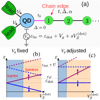
Figure 1: (Color online) (a) Schematic representation of a QD coupled to one end of a topological quantum wire. The quantum wire is described by a tight–binding chain with hopping parameter $t$, Rashba spin–orbit interaction $\alpha$, and induced superconducting pairing $\Delta$. The QD is modeled as a single orbital of energy $\varepsilon_{\text{dot}}$ with local Coulomb interaction $U$, coupled to metallic leads with a coupling $V_{\bf k}$. The energy shift in the QD level from the applied local gate voltage is given by $V_{g}$. An applied magnetic field induces a Zeeman splitting $V_{Z}$ in the wire and $V_{Z}^{(\text{dot})}$ in the QD, where $V_{Z}\neq V_{Z}^{(\text{dot})}$ because of different $g$–factors, $g_{\text{wire}}\neq g_{\text{dot}}$. (b) Single–particle energy level structure of the QD as a function of $V_{Z}^{(\text{dot})}$ for a fixed gate voltage. (c) A spinless regime can be accessed through the application of a large magnetic field in the QD. For comparison with the spinful case $(V_{Z}^{(\text{dot})}=0)$, the spin–down QD level $\varepsilon_{0,\downarrow}$ can be fixed at the energy $\varepsilon_{\text{dot}}$ by simultaneously applying a gate voltage $V_{g}=V_{Z}^{(\text{dot})}$ for positive $V_{Z}^{(\text{dot})}$.

The search for Majorana bound states in condensed matter systems has attracted significant attention in recent years. Most of these investigations have focused on a geometry involving a spin–orbit coupled semiconducting wire with proximity–induced topological ($p$–wave) superconductivity, tunnel coupled to a metallic lead.Alicea (2012) As it is well established theoretically, a finite one–dimensional (1D) topological superconductor sustains zero–energy mid–gap Majorana bound states at its ends.Kitaev (2001) Theory has predicted that these unpaired Majorana bound states—when the hosting superconductor is coupled to normal Fermi liquid leads—can give rise to a zero–bias anomaly in the linear conductance of the system. Mourik et al.Mourik et al. (2012) were the first to report experimental signatures supporting this prediction in conductance measurements through superconductor-normal interfaces. Other theoretical and experimental studiesDeng et al. (2012); Anindya Dasand Ronen et al. (2012); Lee et al. (2012); Churchill et al. (2013); Prada et al. (2012); Rainis et al. (2013); Cook et al. (2012); Liu and Lobos (2013); Stanescu et al. (2011); Lee et al. (2014) have corroborated these findings and, more importantly, have also pointed out a number of alternative possibilities for the appearance of zero–bias anomalies in transport measurements, not at all related to Majorana bound states (e.g., the Kondo effect). A review of these interesting possibilities is provided by Franz in Ref. Franz, 2013.

Alternate routes to realizing Majorana bound states have been proposed, involving magnetic atomic chains with spatially modulated spin textures on the surface of $s$–wave superconductors.Nadj-Perge et al. (2013); Pientka et al. (2013); Klinovaja et al. (2013); Braunecker and Simon (2013); Vazifeh and Franz (2013); Nakosai et al. (2013) In this case, a helical texture emulates the effects of the Zeeman plus spin–orbit fields in the earlier proposals,Fu and Kane (2008); Alicea (2010); Chung et al. (2011); Das Sarma et al. (2012) thus giving rise to Majorana bound states. More recently, a simpler ferromagnetic configuration using self–assembled Fe chains on top of the strongly spin–orbit coupled superconductor Pb has been realized experimentally.Nadj-Perge et al. (2014) The chain ends were probed locally using STM in order to directly visualize the localized modes at the ends of the chain. This experiment is a major step forward in the Majorana search, as compared to previous experimental studies, because it provides the first spatially–resolved possible signature of this elusive state. Note, however, that this experiment, similarly to all previous experiments, cannot unambiguously associate the observed zero–bias feature to the presence of Majorana quasiparticles.Dumitrescu et al. (2015)

A quantum dot (QD) attached to the extremity of a topological wire can also be used to locally probe the emergent Majorana end states, as proposed by Liu and Baranger.Liu and Baranger (2011) These authors considered a setup similar to Fig. 1(a) and found a conductance peak at $0.5e^{2}/h$ for a noninteracting resonant QD (i.e., the dot energy level $\varepsilon_{\rm dot}$ is aligned with the Fermi level $\varepsilon_{F}$ of the leads). Motivated by Ref. Liu and Baranger, 2011, some of us established in Ref. Vernek et al., 2014 that this feature in the QD conductance remains for a wide range of gate voltages $V_{g}$ controlling $\varepsilon_{\rm dot}$, due to the appearance of a resonance pinned at zero bias (i.e., at the Fermi level). This produces a conductance plateau at $0.5\,e^{2}/h$ spanning resonant and off–resonance dot level energies, far above or below $\varepsilon_{F}$.

We argued in Ref. Vernek et al., 2014 that this “0.5” conductance feature was quite distinct from the Kondo effect in quantum dots, as it would appear even for an “empty” dot [$\varepsilon_{dot}(V_{g})>\varepsilon_{F}$]. In that study, however, we had restricted our calculations to a non–interacting spinless model similar to that of Ref. Liu and Baranger, 2011. The natural question is then: How robust are those results, i.e., the “0.5” plateau in the conductance, in the presence of the Coulomb repulsion in the dot? In particular, how is the conductance plateau produced solely by a Majorana mode in the noninteracting dot of our earlier work modified by the Coulomb interaction in the dot, especially in the Kondo regime?

Recent studies have addressed the Kondo regime of a quantum dot coupled to a topological wire and to normal Fermi liquid leadsGolub176802 ; Liu et al. (2015); Lee et al. (2013); Chirla et al. (2014) and to Luttinger leads.Cheng et al. (2014) An important distinction among these studies is whether the topological superconducting wire is grounded or “floating”.footx Our present work and that of Lee et al. in Ref. Lee et al., 2013 consider a floating wire and, with the Majorana mode coupled to the QD spin down degree of freedom, obtain $G_{\downarrow}=0.5\,e^{2}/h$ and $G_{\uparrow}=e^{2}/h$, giving a total conductance of $1.5\,e^{2}/h$ in the Kondo-Majorana regime. In Ref. Liu et al., 2015 the authors also find $G=1.5\,e^{2}/h$ in a similar setup and further calculate the zero–frequency shot noise as an additional probe for the Kondo-Majorana resonance. As we discuss later, the robust pinning $G_{\downarrow}=0.5e^{2}/h$ that we find in the present work for the interacting case corroborates the results of our previous workVernek et al. (2014) and establishes their validity in the interacting case. None of the previous studies have focused on the pinning at “0.5” of the QD conductance as the signature of the leaked Majorana mode in the interacting dot or on the the influence of gate voltages and external magnetic fields on the Majorana-Kondo physics. These are the central goals of our present work.

To address the questions in the previous paragraphs, in this paper we perform a thorough study of the normal-lead–QD–quantum wire system shown schematically in Fig. 1(a). We start off with a realistic model for the wire that explicitly accounts for the Rashba spin–orbit interaction, proximity $s$-wave superconductivity, and a Zeeman term used to drive the wire from its trivial to its topological phase. We study this model with a recursive Green’s function method, using a decoupling procedure known as Hubbard I approximation.Hubbard (1963) This scheme allows us to describe the behavior of the QD for a wide range of parameters in both the trivial and topological phases of the wire. However, the Hubbard I approximation is known to fail when describing the low–temperature regime,Lacroix (1981) hence a nonperturbative treatment is needed. For this purpose we employ the numerical renormalization group (NRG). Because treating the full quantum wire within the NRG is inviable, we adopt a low–energy effective Hamiltonian,Flensberg (2010) in which the realistic wire in its topological phase is replaced by only two Majorana end modes.

We find that in the interacting case, within the Hubbard I approximation, the pinning of the Majorana peak persists for a wide range of gate voltages as long as the dot is empty. However, in the single–occupancy regime of the dot, our mean–field calculations predict that the pinning will be suppressed by Coulomb blockade when the spin up/down states are degenerate. By applying a large Zeeman field in the QD, we drive it into a spinless regime in which Coulomb blockade does not take place and the non–interacting character of the dot is restored with the pinning appearing for both occupied and unoccupied dot as described by our results in Fig. 1(g) of Ref. Vernek et al., 2014.

At low temperatures, in the absence of external Zeeman splitting in the dot, our NRG results show that the Majorana peak in fact appears also in the single–occupancy regime, in agreement with previous NRG studies.Lee et al. (2013) The “leaked” Majorana mode coexists with the Kondo effect for a QD at the particle–hole symmetric point, giving a total zero–bias conductance of $1.5\,e^{2}/h$.Lee et al. (2013) In this situation, we also find that the Majorana–QD coupling strongly enhances the Kondo temperature. In contrast, detuning from the particle–hole symmetric point strongly suppresses the Kondo peak because of an effective Zeeman splitting induced in the QD by the Majorana mode.Lee et al. (2013); Cheng et al. (2014) However, the “0.5” Majorana signature is immune to the Zeeman splitting in the QD, so, far from the particle-hole symmetric point the “0.5” conductance plateau is restored. Further, the Kondo effect can be progressively quenched (even at the particle–hole symmetric point) by an external magnetic field. In this case the resulting zero–bias conductance versus Zeeman energy follows a well–known universal curve. This universal behavior of the conductance for low magnetic fields and the persistent $0.5~{}e^{2}/h$ zero–bias conductance at large magnetic fields are unique pieces of evidence of the Majorana–Kondo physics in the hybrid QD–wire system. We emphasize that even though the phenomenology of interacting dots is much richer than that of their non–interacting counterparts, the QD Majorana resonance pinned to the Fermi level of the leads we have predicted in Ref. Vernek et al., 2014 appears in both cases.

This paper is organized as follows: In Sec. II we introduce the model for the QD–topological quantum wire system. The recursive Green’s function method is explained in Sec. III, and numerical results away from the Kondo regime are shown in Secs. III.2 and III.3. We introduce a low–temperature effective model in Sec. IV and numerically demonstrate its equivalence to the full model in the topological phase. The properties of this model are then investigated using the NRG method in Sec. V. In Sec. VI we discuss the interplay between Majorana and Kondo physics at low temperatures. Finally, an experimental test for this interplay is proposed in Sec. VII. Our conclusions are presented in Sec. VIII.

II Model

Our model consists of a single–level QD, modeled as an atomic site coupled to a finite tight–binding chain that represents the one–dimensional degrees of freedom of the quantum wire [Fig. 1(a)]. The corresponding Hamiltonian is

$$H=H_{\mathrm{dot}}+H_{\mathrm{leads}}+H_{\mathrm{wire}}+H_{\mathrm{dot-leads}}+H_{\mathrm{dot-wire}},$$ (1)

where $H_{\mathrm{dot}}$ describes the isolated QD, $H_{\mathrm{wire}}$ is the Hamiltonian of the wire, and $H_{\mathrm{dot-wire}}$ couples them at one end of the wire. The operator $H_{\mathrm{dot-leads}}$ represents the tunnel coupling of the QD to source and drain metallic leads, which are necessary for transport measurements. The terms describing the QD and the metallic leads are given by

$$H_{\mathrm{dot}}=\sum_{s}\varepsilon_{0,s}c^{\dagger}_{0,s}c_{0,s}+U\,n_{0,\uparrow}n_{0,\downarrow},$$ (2a)

$$H_{\mathrm{leads}}=\sum_{\ell\mathbf{k},s}\varepsilon_{\ell\mathbf{k},s}c^{\dagger}_{\ell\mathbf{k},s}c_{\ell\mathbf{k},s},$$ (2b)

$$H_{\mathrm{dot-leads}}=\sum_{\ell\mathbf{k},s}\left(V_{\ell\mathbf{k}}c^{\dagger}_{0,s}c_{\ell\mathbf{k},s}+V^{*}_{\ell\mathbf{k}}c^{\dagger}_{\ell\mathbf{k},s}c_{0,s}\right),$$ (2c)

where the operator $c^{\dagger}_{0,s}$ ($c_{0,s}$) creates (annihilates) an electron of spin $s$ in the QD; $\varepsilon_{0,\uparrow}=\varepsilon_{\rm dot}+V_{g}+V_{Z}^{({\rm dot})}$ and $\varepsilon_{0,\downarrow}=\varepsilon_{\rm dot}+V_{g}-V_{Z}^{({\rm dot})}$, where $\varepsilon_{\rm dot}$ is the QD energy level; $V_{g}$ represents the level shift by an applied gate voltage; and $V_{Z}^{({\rm dot})}$ is the Zeeman energy induced in the QD by an external magnetic field. Orbital effects from the magnetic field are neglected. The parameter $U$ represents the energy cost for double occupancy of the QD due to Coulomb repulsion, and $n_{0,s}=c^{\dagger}_{0,s}c_{0,s}$ is the QD number operator for spin $s$. The operator $c^{\dagger}_{\ell\mathbf{k},s}$ ($c_{\ell\mathbf{k},s}$) creates (annihilates) an electron with spin $s$, momentum $\mathbf{k}$, and energy $\varepsilon_{\ell\mathbf{k},s}$ in the left ($\ell=L$) or right ($\ell=R$) lead. The coupling constant between the QD and lead $\ell$ is given by $V_{\ell\mathbf{k}}$, and the hybridization function is given by

$$\Gamma(\varepsilon)=\pi\sum_{\ell\mathbf{k},s}\left|V_{\ell\mathbf{k}}\right|^{2}\delta(\varepsilon-\varepsilon_{\mathbf{k}}).$$ (3)

The terms describing the quantum wire and the QD–wire coupling are

$$H_{\mathrm{wire}}=H_{0}+H_{R}+H_{SC},$$ (4a)

$$H_{\mathrm{dot-wire}}=-t_{0}\sum_{s}\left(c^{\dagger}_{0,s}c_{1,s}+c^{\dagger}_{1,s}c_{0,s}\right).$$ (4b)

The chain operator $c^{\dagger}_{j,s}$ ($c_{j,s}$), for $j\geq 1$, creates (annihilates) an electron of spin $s$ at site $j$, and the hopping constant $t_{0}$ couples the QD to the first site of the wire. The terms in $H_{\mathrm{wire}}$ are

$$\begin{split}H_{0}=&\sum_{j=1,s}^{N}\left(-\mu+V_{Z}\sigma^{z}_{ss}\right)c^{\dagger}_{js}c_{js}\\ &-\frac{t}{2}\sum_{j=1,s}^{N-1}\left(c^{\dagger}_{j+1,s}c_{j,s}+c^{\dagger}_{j,s}c_{j+1,s}\right),\end{split}$$ (5)

where $\mu$ is the chemical potential, $\sigma^{z}$ is a Pauli matrix, $t$ is the nearest–neighbor hopping between the sites of the tight–binding chain, and $t_{0}$ is the hopping between the QD and the first chain site. The Zeeman splitting $V_{Z}$ from an external magnetic field (orbital effects are neglected in the wire as well) is assumed to be applied along the $z$ axis, with the wire oriented along the $x$ axis. In principle, $V_{Z}$ can be different from $V_{Z}^{({\rm dot})}$ because of different effective $g$ factors in the wire and the QD.de Sousa and Das Sarma (2003) The length of the wire is given by $aN$, where $N$ is the number of sites and $a$ the lattice constant.

The Rashba spin–orbit Hamiltonian is

$$H_{R}=\sum_{j=1}^{N-1}\sum_{ss^{\prime}}(-it_{\rm SO})c^{\dagger}_{j+1,s}\hat{z}\cdot\left(\vec{\sigma}_{ss^{\prime}}\times\hat{x}\right)c_{j,s^{\prime}}+\text{H.c.},$$ (6)

where $t_{\rm SO}=\sqrt{E_{\rm SO}t}$, $E_{\rm SO}=m^{*}\alpha^{2}/2\hbar^{2}$, $m^{*}$ is the effective electron mass, and $\alpha$ the Rashba spin–orbit strength in the wire.Potter and Lee (2011); Rainis et al. (2013) The proximity–induced $s$–wave superconductivity is described by

$$H_{\mathrm{SC}}=\Delta\sum_{j=1}^{N}\left(c^{\dagger}_{j,\uparrow}c^{\dagger}_{j,\downarrow}+c_{j,\downarrow}c_{j,\uparrow}\right),$$ (7)

where $\Delta$ is the (renormalized) superconducting pairing amplitude, assumed to be real and constant along the wire for simplicity.footy

III Recursive Green’s function calculation

The physical quantity central to our results is the spin–resolved local density of states at any given site (including the QD site), defined as

$$\rho_{j,s}(\varepsilon)=-\frac{1}{\pi}\text{Im}\langle\langle c_{j,s};\,c_{j,s}^{\dagger}\rangle\rangle_{\varepsilon},$$ (8)

where $\langle\langle A;\,B\rangle\rangle_{\varepsilon}$ is the retarded Green’s function of operators $A$ and $B$ in the spectral representation. We now present an iterative procedure for calculating this Green’s function for the Hamiltonian Eq. (4a), using the equation of motion method.Zubarev (1960)

Because of the spin-orbit coupling and the superconducting pairing in $H_{\rm wire}$ [Eq. (4a)], the equation of motion for Eq. (8) couples it to other types of correlation functions involving two creation operators. To accommodate all the needed Green’s functions we define the matrix

$$\begin{split}&{\bf G}_{i,j}(\varepsilon)=\\ &\begin{pmatrix}\langle\langle c_{i,\uparrow};\,c^{\dagger}_{j,\uparrow}\rangle\rangle_{\varepsilon}&\langle\langle c_{i,\uparrow};\,c_{j,\downarrow}^{\dagger}\rangle\rangle_{\varepsilon}&\langle\langle c_{i,\uparrow};\,c_{j,\uparrow}\rangle\rangle_{\varepsilon}&\langle\langle c_{i,\uparrow};\,c_{j,\downarrow}\rangle\rangle_{\varepsilon}\\ \langle\langle c_{i,\downarrow};\,c^{\dagger}_{j,\uparrow}\rangle\rangle_{\varepsilon}&\langle\langle c_{i,\downarrow};\,c^{\dagger}_{j,\downarrow}\rangle\rangle_{\varepsilon}&\langle\langle c_{i,\downarrow};\,c_{j,\uparrow}\rangle\rangle_{\varepsilon}&\langle\langle c_{i,\downarrow};\,c_{j,\downarrow}\rangle\rangle_{\varepsilon}\\ \langle\langle c_{i,\uparrow}^{\dagger};\,c^{\dagger}_{j,\uparrow}\rangle\rangle_{\varepsilon}&\langle\langle c_{i,\uparrow}^{\dagger};\,c_{j,\downarrow}^{\dagger}\rangle\rangle_{\varepsilon}&\langle\langle c_{i,\uparrow}^{\dagger};\,c_{j,\uparrow}\rangle\rangle_{\varepsilon}&\langle\langle c^{\dagger}_{i,\uparrow};\,c_{j,\downarrow}\rangle\rangle_{\varepsilon}\\ \langle\langle c^{\dagger}_{i,\downarrow};\,c^{\dagger}_{j,\uparrow}\rangle\rangle_{\varepsilon}&\langle\langle c^{\dagger}_{i,\downarrow};\,c^{\dagger}_{j,\downarrow}\rangle\rangle_{\varepsilon}&\langle\langle c^{\dagger}_{i,\downarrow};\,c_{j,\uparrow}\rangle\rangle_{\varepsilon}&\langle\langle c^{\dagger}_{i,\downarrow};\,c_{j,\downarrow}\rangle\rangle_{\varepsilon}\end{pmatrix}.\end{split}$$ (9)

We start our iterative procedure by assuming that our system has only the two sites $N$ and $N-1$. Applying the equation of motion to the Green’s function ${\bf G}_{N-1,N-1}(\varepsilon)$ we obtain the Dyson equation (see detailed derivation in Appendix A)

$$\begin{split}{\bf G}_{N-1,N-1}(\varepsilon)=&\,\tilde{\bf g}_{N-1,N-1}(\varepsilon)\\ &+\tilde{\bf g}_{N-1,N-1}(\varepsilon){\bf t}{\bf G}_{N,N-1}(\varepsilon),\end{split}$$ (10)

whose solution is

$${\bf G}_{N-1,N-1}(\varepsilon) = \left[1-\tilde{\bf g}_{N-1,N-1}(\varepsilon){\bf t}\tilde{\bf g}_{N,N}(\varepsilon){\bf t}^{\dagger}\right]^{-1}$$ (11)

$$\times\tilde{\bf g}_{N-1,N-1}(\varepsilon).$$

In Eqs. (10) and (11),

$$\tilde{\bf g}_{N-1,N-1}(\varepsilon)=[1-{\bf g}_{N-1,N-1}(\varepsilon){\bf V}]^{-1}{\bf g}_{N-1,N-1}(\varepsilon),$$

where ${\bf g}_{N-1,N-1}(\varepsilon)$ is the bare Green’s function defined in Eq. (34), while ${\bf V}$ and $\bf t$ are the couplings given in Eqs. (35a) and (35b), respectively.

The Green’s function (11) describes the “effective” site $N-1$ that carries all the information about the site $N$. We are interested, however, in the Green’s function ${\bf G}_{1,1}(\varepsilon)$ that describes an “effective” site $i=1$ carrying the information from all the other $N-1$ sites of the chain (with $N\rightarrow\infty$). To this end, a site $N-2$ is added to the chain and its Green’s function can be evaluated using Eq. (11), with the substitutions $\textbf{G}_{N-1,N-1}\longrightarrow\textbf{G}_{N-2,N-2}$, $\tilde{\textbf{g}}_{N-1,N-1}\longrightarrow\tilde{\textbf{g}}_{N-2,N-2}$, and $\tilde{\textbf{g}}_{N,N}\longrightarrow\textbf{G}_{N-1,N-1}$. The correct description for the quantum wire is reached in the limit $N\gg 1$. This iterative process converges to the large–$N$ limit once the Green’s functions of two subsequent sites $i-1$ and $i$ are identical. In our calculations this was strongly dependent on parameters, but the typical number of sites required for convergence was $N\sim 5\times 10^{4}$.

Once we have reached convergence, the QD is added to the chain as site $i=0$, and the metallic leads are coupled to the QD. The infinite degrees of freedom of the lead electrons are correlated through the local Coulomb interaction in the QD, giving rise to an infinite hierarchy of equations of motion. Therefore, calculating the properties of an interacting QD within the Green’s function formalism unavoidably requires certain approximations in order to truncate this system at finite order. We evaluate the Green’s functions using a method inspired by the Hubbard I decoupling procedure,Hubbard (1963) which allows us to close the recursive system of equations. The resulting Green’s function for the QD is given by (see detailed derivation in Appendix B)

$${\bf g}_{0,0}(\varepsilon)=\begin{bmatrix}\tilde{g}_{0\uparrow,0\uparrow}(\varepsilon)&\frac{A_{g,\uparrow}(\varepsilon)U\langle c^{\dagger}_{0,\downarrow}c_{0,\uparrow}\rangle}{(\varepsilon-\varepsilon_{0,\uparrow})(\varepsilon-\varepsilon_{0,\uparrow}-U)}&0&\frac{A_{g,\uparrow}(\varepsilon)U\langle c_{0,\downarrow}c_{0,\uparrow}\rangle}{(\varepsilon-\varepsilon_{0,\uparrow})(\varepsilon-\varepsilon_{0,\uparrow}-U)}\\ \frac{A_{g,\downarrow}(\varepsilon)U\langle c^{\dagger}_{0,\uparrow}c_{0,\downarrow}\rangle}{(\varepsilon-\varepsilon_{0,\downarrow})(\varepsilon-\varepsilon_{0,\downarrow}-U)}&\tilde{g}_{0\downarrow,0\downarrow}(\varepsilon)&\frac{A_{g,\downarrow}(\varepsilon)U\langle c_{0,\uparrow}c_{0,\downarrow}\rangle}{(\varepsilon-\varepsilon_{0,\downarrow})(\varepsilon-\varepsilon_{0,\downarrow}-U)}&0\\ 0&\frac{A_{h,\uparrow}(\varepsilon)U\langle c^{\dagger}_{0,\uparrow}c^{\dagger}_{0,\downarrow}\rangle}{(\varepsilon+\varepsilon_{0,\uparrow})(\varepsilon+\varepsilon_{0,\uparrow}+U)}&\tilde{h}_{0\uparrow,0\uparrow}(\varepsilon)&\frac{A_{h,\uparrow}(\varepsilon)U\langle c_{0,\downarrow}c^{\dagger}_{0,\uparrow}\rangle}{(\varepsilon+\varepsilon_{0,\uparrow})(\varepsilon+\varepsilon_{0,\uparrow}+U)}\\ \frac{A_{h,\downarrow}(\varepsilon)U\langle c^{\dagger}_{0,\downarrow}c^{\dagger}_{0,\uparrow}\rangle}{(\varepsilon+\varepsilon_{0,\downarrow})(\varepsilon+\varepsilon_{0,\downarrow}+U)}&0&\frac{A_{h,\downarrow}(\varepsilon)U\langle c_{0,\uparrow}c^{\dagger}_{0,\downarrow}\rangle}{(\varepsilon+\varepsilon_{0,\downarrow})(\varepsilon+\varepsilon_{0,\downarrow}+U)}&\tilde{h}_{0\downarrow,0\downarrow}(\varepsilon)\end{bmatrix},$$ (13)

with the definitions $A_{g,s}(\varepsilon)=[1+i\Gamma g_{0s,0s}(\varepsilon)]^{-1}$, $A_{h,s}(\varepsilon)=[1+i\Gamma h_{0s,0s}(\varepsilon)]^{-1}$, $\tilde{g}_{0s,0s}(\varepsilon)=A_{g,s}(\varepsilon)g_{0s,0s}(\varepsilon)$, and $\tilde{h}_{0s,0s}(\varepsilon)=A_{h,s}(\varepsilon)h_{0s,0s}(\varepsilon)$, where

$$g_{0s,0s}(\varepsilon)=\frac{1-\langle n_{0,\bar{s}}\rangle}{\varepsilon-\varepsilon_{0,s}}+\frac{\langle n_{0,\bar{s}}\rangle}{\varepsilon-\varepsilon_{0,s}-U},$$ (14)

and

$$h_{0s,0s}(\varepsilon)=\frac{1+\langle n_{0,\bar{s}}\rangle}{\varepsilon+\varepsilon_{0,s}}-\frac{\langle n_{0,\bar{s}}\rangle}{\varepsilon+\varepsilon_{0,s}+U}.$$ (15)

Note that this approach requires the self–consistent calculation of the various local expectation values appearing in Eq. (13), such as the occupation of the QD $\langle n_{0,s}\rangle$, the spin–flip expectation value $\langle c^{\dagger}_{0,s}c_{0,\bar{s}}\rangle$, and the pairing fraction $\langle c^{\dagger}_{0,s}c^{\dagger}_{0,\bar{s}}\rangle$. The last two quantities result from the spin–flip processes induced by the spin–orbit interaction and the $s$-wave pairing in the wire, respectively. Since these quantities are indirectly induced on the QD via its coupling to the wire, compared to the occupations of the dot, they are small quantities and can be neglected. To confirm this we have numerically evaluated their contributions for a wide range of parameters. The main effect of these terms is to delay the convergence of the self–consistent calculation.

III.1 Topological phase transition for the quantum wire

For our numerical calculations we follow previous studiesMourik et al. (2012); Rainis et al. (2013) and use the following parameters for the quantum wire: $t=10~{}{\rm meV}$, $E_{\rm SO}=50~{}\mu{\rm eV}$, $\Delta=250~{}\mu{\rm eV}$, and $\tilde{\mu}=-0.01t$. As discussed in detail in Ref. Alicea, 2012, the condition for the topological phase, where the wire sustains Majorana end states, is $|V_{Z}|>\sqrt{\tilde{\mu}^{2}+\Delta^{2}}\equiv|V_{Z}^{c}|$. For our parameters the topological phase transition occurs for $V_{Z}\approx\pm 250\,\mu{\rm eV}$.

In the remainder of this section, as well as in Secs. III.2 and III.3, we maintain this set of parameters and work exclusively in the topological phase by setting the Zeeman splitting in the wire to $V_{Z}=500\,\mu{\rm eV}$. The QD–leads hybridization is assumed constant and set to $\Gamma=1~{}\mu{\rm eV}$, and the QD–wire coupling is set to $t_{0}=40\,\Gamma$. This choice of $t_{0}>\Gamma$ ensures that the hybridization to the leads does not smear out any features of the density of states introduced by the coupling to the wire. The Fermi level of the leads is set as the energy reference, $\varepsilon_{F}=0$.

Let us begin with a general survey of the QD density of states (DOS) when the wire is driven from its trivial to its topological phase, by increasing $V_{Z}>0$. Figure 2 shows a color map of the total QD DOS ($\rho_{\uparrow}+\rho_{\downarrow}$) versus the energy $\varepsilon$, and the Zeeman energy in the wire $V_{Z}$. Henceforth we use the abbreviation $\rho_{s}\equiv\rho_{0,s}$ for the QD DOS. The left [Figs. 2(a) and 2(b)] and right [Figs. 2(c) and 2(d)] panels correspond to $U=0$ and $U=12.5\Gamma$, respectively. The top and bottom panels are, respectively, the DOS for $V_{Z}^{\rm(dot)}=0$ and $V_{Z}^{\rm dot}=0.1V_{Z}$. For a clear comparison among the four different cases we fix the lowest energy QD level—in this case $\varepsilon_{0,\downarrow}$, due to the positive Zeeman splitting—to an energy $\varepsilon_{\text{dot}}=-6.25\,\Gamma$ (see Sec. III.3). This is achieved with the application of a gate voltage $V_{g}=V_{Z}^{(\text{dot})}$, as shown in Fig. 1(c).

The general features of the DOS are as follows: In Fig. 2(a) the colored band fixed at $\varepsilon=-6.25\,\Gamma$ corresponds to the spin–degenerate QD levels $\varepsilon_{0,s}$. When $V_{Z}^{(\text{dot})}=0.1\,V_{Z}$ [Fig. 2(b)] this degeneracy is broken, and the spin–up level $\varepsilon_{0,\uparrow}$ is seen moving to higher energies as the bright diagonal band on the left of the panel. The spin–down level is, as mentioned before, kept in place by a gate voltage $V_{g}=V_{Z}^{(\text{dot})}$. For $U=12.5\,\Gamma$ and $V_{Z}^{(\text{dot})}=0$ [Fig. 2(c)] the spin degeneracy is restored, and so is the bright feature at $\varepsilon\approx-6.25\,\Gamma$. In addition, a second bright band appears at $\varepsilon\approx\varepsilon_{0,s}+U=6.25\,\Gamma$, corresponding to the doubly occupied state of the QD. When a large Zeeman field is introduced [Fig. 2(d)] both bands split, shifting both the spin–up and the doubly occupied states to high energies, effectively eliminating them from the picture.

A sharp peak (indicated with arrows) appears at the Fermi level after the topological transition $V_{Z}>V_{Z}^{c}$ (indicated with the vertical dashed line) in Figs. 2(a), 2(b) and 2(d). That is, the zero–bias signature appears for a non–interacting QD ($U=0$) for both a zero and a large magnetic field [$V_{Z}^{(\text{dot})}=0$ and $V_{Z}^{(\text{dot})}=0.1\,V_{Z}$] and for an interacting QD ($U=12.5\,\Gamma$) in the case of a large magnetic field. Note, however, that for $U=12.5\,\Gamma$ and $V_{Z}^{\rm(dot)}=0$ [Fig. 2(c)] the topological phase transition appears to occur at higher $V_{Z}\approx 0.4\,{\rm meV}$. Moreover, after this apparent transition the central peak is strongly suppressed and shifted to negative energies.

The parameters used in Fig. 2(c) suggest that these effects may be a consequence of the Coulomb blockade within the QD. As mentioned above, when a large $V_{Z}^{(\text{dot})}$ is applied the spin–up and the doubly occupied states are pushed to high energies. For $V_{Z}\gtrsim V_{Z}^{c}$ these states no longer partake in the low–energy physics of the problem, and we are left with a spinless, noninteracting model. In this situation the zero–bias peak reappears.

As we discuss below, this peak is associated with the formation of Majorana zero modes $\gamma_{1}$ and $\gamma_{2}$ at the ends of the wire. The mode $\gamma_{1}$ located close to the QD “leaks” into the dot, producing a spectral signature pinned to the Fermi level for a wide variety of QD parameters, in agreement with our previous resultsVernek et al. (2014) for a non-interacting model. The results of Fig. 2(d) might suggest that the Coulomb interaction prevents the Majorana mode from entering the QD for small values of $V_{Z}$. As we discuss in the following sections, this picture changes when Kondo correlations are correctly taken into account within the NRG approach.

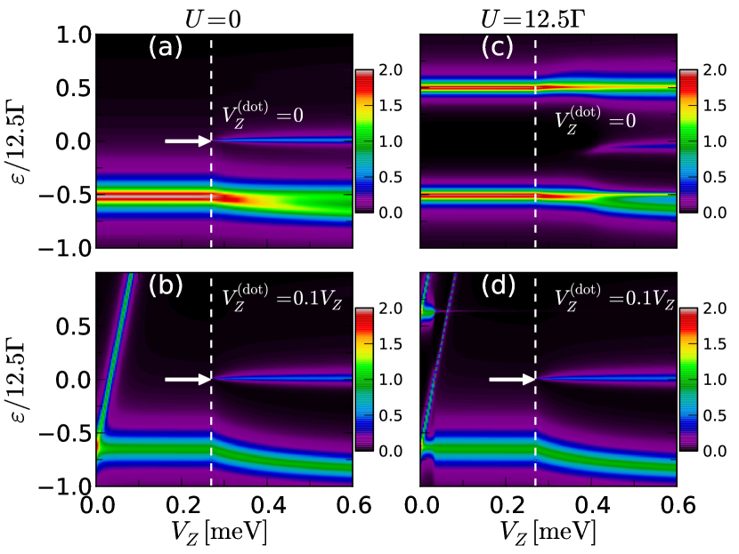
Figure 2: (Color online) Density of states at the QD site as a function of the Zeeman splitting in the wire, calculated using the Hubbard I method. The top panels [(a) and (c)] are for the QD factor $g_{\text{dot}}=0$, whereas the bottom panels [(b) and (d)] correspond to $g_{\text{dot}}=0.1\,g_{\text{wire}}$. Results for the noninteracting case ($U=0$) are presented in panels (a) and (b); results for the interacting case are shown in panels (c) and (d). These calculations are carried out with the QD spin–down level fixed at $\varepsilon_{0,\downarrow}=\varepsilon_{\text{dot}}$. For this purpose, a compensating gate voltage $V_{g}=V_{Z}^{(\text{dot})}$ is applied (see the discussion in Sec.  III.3). Parameters: $t=10~{}{\rm meV}$, $E_{\rm SO}=50~{}\mu{\rm eV}$, $\Delta=250~{}\mu{\rm eV}$, $\tilde{\mu}=-0.01t$; $\Gamma=1~{}\mu{\rm eV}$, $\varepsilon_{\text{dot}}=-6.25\,\Gamma$, and $t_{0}=40\,\Gamma$.

III.2 Numerical results for $V_{Z}^{(\text{dot})}=0$

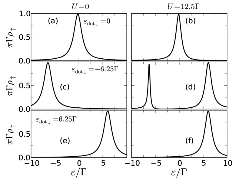
Figure 3: Spin–up local density of states of the QD for the wire in the topological phase, with $t=10~{}{\rm meV}$, $E_{\rm SO}=50~{}\mu{\rm eV}$, $V_{Z}=500~{}\mu{\rm eV}$, and $\tilde{\mu}=-0.01t$. QD parameters are $\Gamma=1~{}\mu{\rm eV}$ and $t_{0}=40\Gamma$.

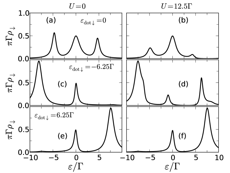
Figure 4: Spin–down local density of states of the QD for the wire in the topological phase, for the same parameters of Fig. 4. Note the reduced amplitude and the shift toward negative energies of the central peak in panel (d), for finite $U$ and $\varepsilon_{0,s}<0$.

Figures 4 and 4 show the spin–up and spin–down local DOS at the QD site, respectively, with the wire in the topological regime, and in the absence of a Zeeman splitting in the QD [$V_{Z}^{(\mathrm{dot})}=0$]. The results for an interacting ($U=12.5\Gamma$) and a noninteracting ($U=0$) QD are presented side by side for comparison.

The spin–up density of states in Fig. 4 shows the usual structure of a QD level: In the non–interacting case there is a single Lorentzian peak of width $\Gamma$ and centered at $\varepsilon=\varepsilon_{\mathrm{dot}}$, produced by the dot level dressed by the electrons of the leads. Two Hubbard bands appear in the interacting case, at $\varepsilon\approx\varepsilon_{\text{dot}}$ and $\varepsilon\approx\varepsilon_{\text{dot}}+U$ (the double occupancy excitation), but there are no additional features from the coupling to the quantum wire in either case. This is a consequence of the large, positive Zeeman field $V_{Z}$ in the wire, which effectively decouples it from the spin–up level in the QD. Had we chosen a negative field $V_{Z}$, the spin–up level in the QD would decouple instead.

The signature of the Majorana zero mode forming at the end of the quantum wire appears in the QD spin–down density of states $\rho_{\downarrow}$ (Fig. 4), as an additional resonance of amplitude $0.5$ (in units of $1/\pi\Gamma$) pinned to the Fermi level. In the noninteracting case, this resonance is robust to the applied gate voltage [Figs. 4(a), 4(c) and 4(e)], in agreement with our results for a spinless model presented in Ref. Vernek et al., 2014 and also with Ref. Liu and Baranger, 2011. The “0.5” signature remains in the interacting case for $\varepsilon_{0,s}\geq 0$ [Figs. 4(b) and 4(f)], and no additional features are observed in $\rho_{\downarrow}$ (apart from the two usual Hubbard bands). However, for $\varepsilon_{0,s}=-U/2$ [Fig. 4(d)], and in general for $\varepsilon_{0,s}<0$, with $|\varepsilon_{0,s}|\gg\Gamma$ (not shown), the central peak appears with a reduced amplitude ($<0.5$) and shifted toward negative energies. For $V_{Z}<0.4\mu{\rm eV}$ [e.g., Fig. 2(c)], the peak can in fact be completely suppressed because of the Coulomb blockade in the dot. Again, we remark that this is an artifact of the Hubbard I approximation that is unable to correctly describe the ground state of the system.

III.3 Numerical results for $V_{Z}^{(\text{dot})}\gg U$

The only difference between the cases of Fig. 4(c) (where the “0.5” resonance appears) and Fig. 4(d) (where it does not) is the Coulomb interaction at the QD site. Indeed, the Coulomb interaction plays a role only when the dot is singly occupied, and there is the possibility for a second electron to hop into the dot (with an energy cost $U$). This is the situation when $\epsilon_{0,s}<\varepsilon_{F}$ and $\epsilon_{0,s}+U>\varepsilon_{F}$. The Coulomb blockade effect is suppressed, for instance, when the Zeeman energy prevents one of the spin species to hop into the dot, for example, if $\varepsilon_{0,\downarrow}<\varepsilon_{F}$ and $\varepsilon_{0,\uparrow}>\varepsilon_{F}$ [see Figs. 1(b) and 1(c)]. In this case, the second electron (with spin $\uparrow$) is prevented from hopping into the dot, not because of the Coulomb repulsion, but because of the Zeeman energy.

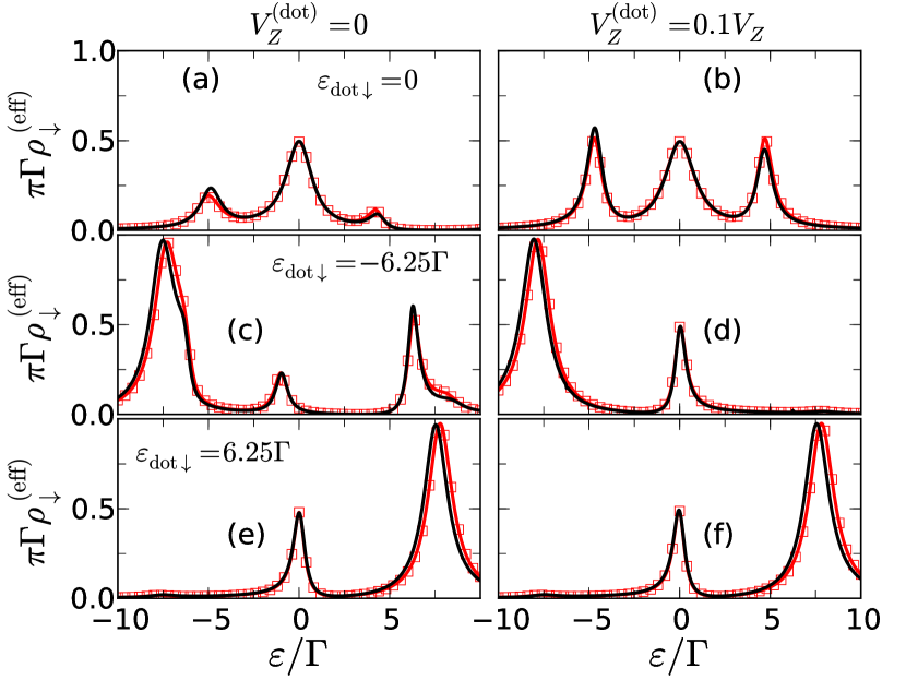
Figure 5: (Color online) Spin–down local density of states at the QD site for the microscopic model Eq. (2) (solid line) and for the effective model Eq. (16) (squares). The parameters are the same as in Fig. 4 but with a finite Zeeman energy $V_{Z}^{({\rm dot})}=0.1V_{Z}=50\mu{\rm eV}$. A gate voltage $V_{g}=V_{Z}^{(\text{dot})}$ is also applied in order to fix $\varepsilon_{0,\downarrow}=\varepsilon_{\text{dot}}$ for comparison with Fig. 4.

In Fig. 5 we shown the spin–down density of states with an applied Zeeman field $V_{Z}^{(\mathrm{dot})}=0.1\,V_{Z}$ within the QD, introduced to suppress the Coulomb blockade within the single–occupancy regime. The field raises (lowers) the spin–up (spin–down) level to $\varepsilon_{0,\uparrow}=\varepsilon_{\mathrm{dot}}+V_{Z}^{(\mathrm{dot})}$ ($\varepsilon_{0,\downarrow}=\varepsilon_{\mathrm{dot}}-V_{Z}^{(\mathrm{dot})}$), producing a total Zeeman splitting of $2V_{Z}^{(\mathrm{dot})}$. We want to compare the results for the $\rho_{\downarrow}$ with finite $V_{Z}^{(\mathrm{dot})}$ with those for $V_{Z}^{(\mathrm{dot})}=0$ shown in Fig. 4. Since now $\varepsilon_{0,\downarrow}$ is shifted by $-V_{Z}^{\rm(dot)}$, we adjust the gate voltage for every value of $V_{Z}^{(\mathrm{dot})}$ as $V_{g}=V_{Z}^{(\mathrm{dot})}$, so the peak of $\rho_{\downarrow}$ at $\varepsilon=\varepsilon_{0,\downarrow}$ appears always in the same place, regardless of the Zeeman energy strength in the QD. This same procedure, which does not pose any major experimental difficulties, was followed in Fig. 2, and is sketched in Figs. 1(b) and (c).

The large magnetic field and gate voltage ($V_{g}=V_{Z}^{(\mathrm{dot})}>U$) push the spin–up level and the doubly occupied state to much higher energies. These are the bright diagonal lines seen in Figs. 2(b) and 2(d) moving out of the frame. This makes $\rho_{\uparrow}=0$ in the relevant energy range and renders the electron–electron interaction irrelevant. At this point we are left with an effectively spinless model [Fig. 1(c)]. As expected, the large magnetic field brings the central peak to the Fermi level and restores its amplitude. This can be seen by comparing Figs. 5(d) and 4(d).

These results indicate that the suppression of the “0.5” peak in the case of Fig. 4(d) is related to the Coulomb blockade effect, at a Hartree level. This, however, should be taken with caution: As we mentioned above, the evaluation of the Green’s function for the interacting QD requires an approximation in order to close the hierarchy of equations of motion. For this purpose, the Hubbard I method uses a mean–field approach, which by definition neglects important many–body correlations introduced by the Coulomb interaction. Thus, the observed behavior of the central peak in the Coulomb blockade regime may well be an artifact of the method. In Sec. V we demonstrate that this is, in fact, the case. To properly take into account the many–body correlations we use the NRG method for the low-temperature regime. However, within the NRG approach we cannot handle the full realistic model for the wire. We then use an effective low-energy model capable of describing the wire in its topological phase. This effective model is described next.

IV Effective model

In this section we discuss the equivalence of the full model Eq. (1) in the topological phase to an effective Hamiltonian in which only the emergent Majorana end state is directly coupled to the QD. This effective model has been used in the literature to describe hybrid QD–topological quantum wire systems, representing the wire only in terms of its Majorana end states.Golub176802 ; Lee et al. (2013); Cheng et al. (2014) To our knowledge, its equivalence to the full microscopic model has never been demonstrated.

The effective model has been employed recently in the non–interacting QD limit, in which case its DOS and transport properties can be calculated analytically.Liu and Baranger (2011) Here, we include the Coulomb interaction in the QD site and use the Hubbard I approximation to close the infinite hyerarchy of equations of motion resulting from it. We evaluate its corresponding DOS $\rho_{s}^{\text{eff}}(\varepsilon)$ and compare it with the results of Secs. III.2 and III.3, showing that all QD spectral features are correctly reproduced for an appropriate choice of the QD–Majorana parameter $\lambda$ (Fig. 5).

The results of Sec. III.2 demonstrate that only the QD spin–down channel couples to the quantum wire in the topological phase when $V_{Z}>0$. In this situation the effective model is given by

$$\begin{split}H_{\rm eff}=&\sum_{s}\varepsilon_{0,s}c^{\dagger}_{0,s}c_{0,s}+U\,n_{0,\uparrow}n_{0,\downarrow}+\lambda\left(c_{0,\downarrow}-c^{\dagger}_{0,\downarrow}\right)\gamma_{1}\\ &+H_{\mathrm{leads}}+H_{\mathrm{dot-leads}},\end{split}$$ (16)

where $\gamma_{1}$ is the operator for the Majorana bound state at the end of the wire, $\lambda$ is the coupling between the dot and the Majorana end mode and $H_{\mathrm{leads}}$ and $H_{\mathrm{dot-leads}}$ are defined in Eqs. (2b) and (2c), respectively.

By using the equation of motion technique we derive the following closed expression for the spin–down Green’s function at the QD site, within the Hubbard I approximation (Appendix B):

$$\langle\langle c_{0\downarrow};\,c^{\dagger}_{0\downarrow}\rangle\rangle_{\varepsilon}=\frac{\tilde{g}_{0\downarrow,0\downarrow}(\varepsilon)\left[\varepsilon-2\lambda^{2}\tilde{h}_{0\downarrow,0\downarrow}(\varepsilon)\right]}{\varepsilon-2\lambda^{2}\tilde{g}_{0\downarrow,0\downarrow}(\varepsilon)-2\lambda^{2}\tilde{h}_{0\downarrow,0\downarrow}(\varepsilon)}.$$ (17)

The peak structure of the density of states $\rho^{(\rm eff)}_{\downarrow}(\varepsilon)$ is the same as that from the microscopic model. For the set of parameters used in Fig. 4 we found that $\lambda=t_{0}/17$ quantitatively reproduces the results of the full chain in both the interacting (Hubbard-I) and the non–interacting (not shown) cases. This is presented in Fig. 5, where the density of states of the effective model is plotted in squares.

In the specific case of a large Zeeman field $V_{Z}^{(\mathrm{dot})}$ [Figs. 5(b), 5(d) and 5(f)], the recovery of the central peak in the microscopic model is also reproduced by the effective model, as can be seen in Fig. 5(d). Moreover, the Green’s function Eq. (17) gives further insight into the behavior of the “0.5” resonance in the Coulomb blockade regime.

As the spin–up density of states $\rho_{\uparrow}^{(\text{eff})}$ vanishes due to the large Zeeman splitting, so does the ground–state spin–up occupancy, given by

$$\langle n_{0,\uparrow}\rangle=\int_{-\infty}^{\infty}\mathrm{d}\omega\,\rho_{\uparrow}(\omega)f(\omega,\,T),$$ (18)

with $f(\omega,\,T)$ the Fermi function. This directly relates to the “0.5” resonance in the spin–down density of states. At $\varepsilon=0$, Eq. (17) can be written as

$$\begin{split}\langle\langle c_{0\downarrow};\,c^{\dagger}_{0\downarrow}\rangle\rangle_{\varepsilon=0}=\frac{1}{[g_{\downarrow}(0)]^{-1}+[h_{\downarrow}(0)]^{-1}+2i\Gamma},\end{split}$$ (19)

whose density of states is a Lorentzian peak centered at the Fermi level only if $[g_{\downarrow}(0)]^{-1}+[h_{\downarrow}(0)]^{-1}=0$, that is, if

$$\frac{\varepsilon_{0,\downarrow}(\varepsilon_{0,\downarrow}+U)}{\varepsilon_{0,\downarrow}+U(1+\langle n_{0,\uparrow}\rangle)}-\frac{\varepsilon_{0,\downarrow}(\varepsilon_{0,\downarrow}+U)}{\varepsilon_{0,\downarrow}+U(1-\langle n_{0,\uparrow}\rangle)}=0.$$ (20)

Equation (20) is satisfied for arbitrary $\varepsilon_{0,\downarrow}$ only when $U=0$, or $\langle n_{0,\uparrow}\rangle=0$. The latter is precisely the case in Fig. 5(d).

The excellent agreement between the effective model and the results of Secs. III.2 and III.3 shows that the effective model captures the Majorana feature both in the non–interacting and in the interacting regime within the Hubbard I approximation. In Sec. V we study the Kondo regime of the Majorana–QD system with NRG method.Wilson (1975); Krishna-murthy et al. (1980a, b)

For a typical QD–lead system, not coupled to the quantum wire, the NRG method relies on the mapping of the itinerant electron degrees of freedom into a tight–binding chain, where each site represents a given energy scale. This energy scale decreases exponentially with the “distance” between the QD and the chain site.Wilson (1975); Krishna-murthy et al. (1980a) For our hybrid QD–quantum wire sytem, however, the gapped nature of the topological superconducting wire prevents us from doing this mapping, which is fundamental for treating the leads and the wire on equal footing. This is not a problem for the effective model, where the topological property of the quantum wire is represented simply as a Majorana state.

V Kondo Regime

As mentioned in Sec. III.2, the Hubbard I method makes use of a mean–field approximation [Eq. 44] which systematically neglects the many–body correlations introduced by the local Coulomb interaction within the QD. This is a good approximation at high temperatures, and it allows us to describe the system both in and out of the topological phase, as a function of all of the quantum wire parameters. However, for the parameters of Figs. 4(d) and 4(d), these correlations are known to give rise to the Kondo effect,Goldhaber-Gordon et al. (1998) which in a typical QD (not coupled to the quantum wire) dominates the behavior of the system below a characteristic temperature scale $T_{K}$, known as the Kondo temperature.Abrikosov (1965) In this low–temperature regime the Hubbard I approximation is at a loss, and the study of the Majorana–QD system requires a method which can fully describe these low–energy correlations.

In this section we employ the NRG to study the effective Hamiltonian Eq. (16), which describes the relevant degrees of freedom of the quantum wire in terms only of the emergent Majorana zero mode at its end and its coupling to the QD, $\lambda$.

The NRG is a fully nonperturbative technique tailor–made to treat many–body correlations in quantum impurity problems.Krishna-murthy et al. (1980a, b) It makes use of a logarithmic discretization of the leads’ energy continuum to thoroughly sample the energy scales closest to the Fermi level, which are the most relevant for the Kondo effect.Wilson (1975); Bulla et al. (2008) However, a well–known limitation of this discretization scheme is the relatively poor description of high–energy spectral features, such as Hubbard bands. Thus the NRG and the Hubbard I results complement each other for a full description of the system at hand.

The effective model can be written as a two–site interacting quantum impurity with a local superconducting pairing term, coupled to metallic leads

$$\begin{split}H_{\rm eff}=&H_{\text{dot}}+H_{\mathrm{leads}}+H_{\mathrm{dot-leads}}\\ &+\lambda\left(c^{\dagger}_{0,\downarrow}f_{\downarrow}+c^{\dagger}_{0,\downarrow}f^{\dagger}_{\downarrow}+\text{H.c.}\right),\end{split}$$ (21)

where $H_{\text{dot}}$, $H_{\mathrm{leads}}$, and $H_{\mathrm{dot-leads}}$ are defined in Eq. (2), and the operator $f_{\downarrow}=\left(\gamma_{1}+i\gamma_{2}\right)/\sqrt{2}$ represents a regular fermion associated with the Majorana bound states in the wire. Its number operator is given by $n_{f,\downarrow}=f_{\downarrow}^{\dagger}f_{\downarrow}$.

One can readily see that the last term in the Hamiltonian Eq. (21) does not preserve the total charge $\hat{N}=n_{0,\uparrow}+n_{0,\downarrow}+n_{f}$, or the total spin projection $S_{z}=(n_{0,\uparrow}-n_{0,\downarrow}-n_{f,\downarrow})/2$. However, defining $\hat{N}_{s}$ as the total number of fermions with spin index $s$, we see that Eq. (21) preserves $\hat{N}_{\uparrow}$ and the parity defined by the operator $\hat{P}_{\downarrow}\equiv(-1)^{\hat{N}_{\downarrow}}$. That is, the even or odd ($+1$ or $-1$) parity of the number of spin–down fermions in the Majorana–QD–leads system. This choice of quantum numbers considerably simplifies the NRG calculations, as noted in Ref. Lee et al., 2013. In order to calculate the spectral properties of the model, we use the density matrix NRG (DM–NRG) method.Hofstetter (2000)

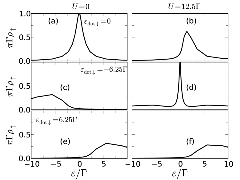
Figure 6: NRG calculations of the zero–temperature spin–up local density of states at the QD site, in the absence of a magnetic field ($V_{Z}^{(\text{dot})}=0$). The interacting (noninteracting) case is presented in the right (left) panels, where the Coulomb interaction is $U=12.5\Gamma$ ($U=0$). The QD level position is indicated in the panels, and the Majorana–QD coupling is $\lambda=0.707\,\Gamma$.

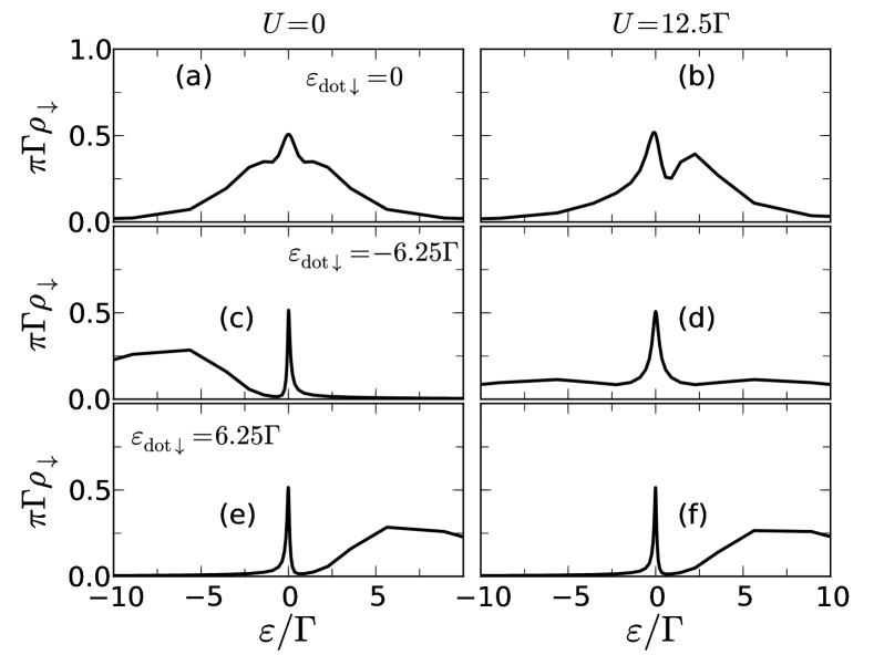
Figure 7: NRG calculations of the zero–temperature spin–down local density of states at the QD site, in the absence of a magnetic field ($V_{Z}^{(\text{dot})}=0$). The interacting (noninteracting) case is presented in the right (left) panels, where the Coulomb interaction is $U=12.5\Gamma$ ($U=0$). The QD level position is indicated in the panels, and the Majorana–QD coupling is $\lambda=0.707\,\Gamma$.

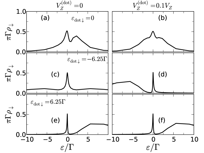
Figure 8: NRG calculations of the zero–temperature spin–down local density of states at the QD site, in the presence of a strong Zeeman field $V_{Z}^{(\text{dot})}$ within the QD. Parameters: $U=12.5\,\Gamma$, $\lambda=\Gamma$.

The spin–resolved DOS $\rho_{\uparrow}(\varepsilon)$ and $\rho_{\downarrow}(\varepsilon)$ are shown in Figs. 7 and 7, respectively. For comparison with Figs. 4 and 4, the left panels of each figure show the results for the noninteracting case ($U=0$), whereas the interacting case ($U>0$) is presented in the right panels.

By construction, the spin–up channel has no direct coupling to the Majorana degrees of freedom. As a consequence, the spin–up spectral density in the noninteracting case (Figs. 7, left panels) shows only the usual Hubbard band at $\varepsilon_{0,\uparrow}$. Comparing to the corresponding panels of Fig. 4, we can see that the position of the Hubbard band for each case is consistent in both calculations, although the peak is somewhat excessively broadened in the DM-NRG calculations, a known limitation of the broadening procedure from the discrete NRG spectral data.Žitko (2011)

The most important differences appear in the interacting case (Fig. 7, right panels). For $\varepsilon_{0,\uparrow}=0$, the Hubbard I approximation predicts a peak in the density of states at the Fermi energy ($\varepsilon=0$), as can be seen in Fig. 4(b). This corresponds to the QD spin–up level, dressed by the electrons from the leads. That is not the case for the NRG results, where the QD energy level appears shifted away from $\varepsilon=0$ and toward positive energies [Fig. 7(b)] due to the particle–hole asymmetry introduced by the Coulomb interaction in the case of $\varepsilon_{0,\sigma}=0$.

For $\varepsilon_{0,\uparrow}=-6.25\,\Gamma$ the QD is in the single–occupancy regime, where the Kondo effect occurs at temperatures below $T_{K}$. This is signaled by the appearance of a sharp peak of amplitude $(\pi\Gamma)^{-1}$ and width $\sim T_{K}$ at the Fermi level in Fig. 7(d), typical of the Kondo ground state. It should be noted that these results correspond to $\varepsilon_{0,s}=-U/2$, where the QD has particle–hole symmetry. When there is some detuning $\delta$ from the particle–hole symmetric point, such that $\varepsilon_{0,s}=-U/2+\delta$, an effective Zeeman splitting of strength $8|\delta|\lambda^{2}/U^{2}$ is known to arise in the QD because the Majorana mode couples exclusively to one spin channel.Lee et al. (2013) The Kondo effect is quenched when this splitting is larger than the Kondo temperature. This is in stark contrast to the results of Fig. 4(d), where the Hubbard I approximation predicts simply a Coulomb blockade gap for all $-U<\varepsilon_{0,s}<0$.

We now turn to the spin–down DOS, presented in Fig. 7. The signature of the Majorana mode “leaking” into the QD can be seen both in the interacting and in the non–interacting case, and for all values of $\varepsilon_{0,\downarrow}$. In the absence of interactions, the NRG calculation confirms the results from the Hubbard I approximation: For $\varepsilon_{0,\downarrow}=0$, shown in Fig. 7(a), the same three–peak structure of Fig. 4(a) is observed, albeit with wider side peaks. Our reasons for using a smaller value of $\lambda$ become clear in this case: The side bands in Fig. 7(a) appear at positionsLiu and Baranger (2011) $\varepsilon=\pm\lambda$. By using a small $\lambda$ we keep them closer to the Fermi level, where they are better resolved by our NRG results. In Figs. 7(c) and 7(e) we observe the expected Hubbard bands centered at $\varepsilon=\pm 6.5\,\Gamma$, but, more importantly, the “0.5” peak pinned at the Fermi level. This is also in good agreement with the results of Figs. 4(c) and 4(e).

As in the case of the spin–up density of states, there are important differences between the results from the two methods in the interacting case. For $\varepsilon_{0,\downarrow}=0$, the Hubbard I results predict that the three–peak structure seen in the noninteracting case remains in the presence of the Coulomb interaction; the “0.5” peak remains intact and the amplitudes for both side bands are reduced [Fig. 4(b)]. In contrast, the NRG results of Fig. 7(b) demonstrate that the side bands are shifted to positive energies, as in the case of the spin up level in Fig. 7(b). The left side band is strongly reduced and mixes with the tail of the “0.5” central peak, which remains pinned to the Fermi level in the presence of the Coulomb interaction.

Figure 7(d) shows that the “0.5” peak persists even in the single–occupancy regime ($\varepsilon_{0,\downarrow}=-6.5\,\Gamma$), where in a typical QD (in the absence of the wire) the Kondo peak would be expected. We emphasize that the NRG method is particularly accurate at energies close to the Fermi level, and that it correctly describes this signature of the Majorana mode. This important result has also been found by Lee et al.;Lee et al. (2013) it demonstrates that the Majorana ground state dominates over the Kondo effect at zero temperature and that the signature is robust to the effects of the Coulomb interaction in the QD. This was recently discussed in Ref. Cheng et al., 2014, using an analytical renormalization group analysis of a similar system in the weak QD–Majorana coupling limit. There it was suggested that a new low–energy Majorana fixed point emerges, which dominates over the usual (Kondo) strong–coupling fixed point. This picture is certainly supported by our results.

For completeness, we evaluate also the spin–down density of states in the limit of a large Zeeman field in the interacting QD [$V_{Z}^{(\text{dot})}\gg U>0$] for comparison with the results presented in Fig. 5. As discussed in Sec. III.3, the combination of the positive Zeeman splitting and the gate voltage holding the spin–down level in place raises the spin–up level to high energies. This effectively freezes the spin–up and the double occupancy states, restoring the noninteracting picture and eliminating the possibility for the Kondo effect. This is shown in the right panels of Fig. 8. Figures 8(a), 8(c) and 8(e) show the same results as the corresponding panels of Fig. 7 for side by side comparison. As expected, the large magnetic field restores the results for a noninteracting QD, presented in the left panels of Fig. 7. This is consistent with the Hubbard I results of Fig. 5.

VI Separating the Kondo–Majorana ground state

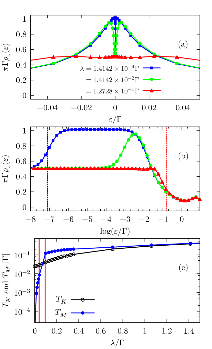
Figure 9: (Color online) Extracting the Majorana energy scale $T_{M}$ from the spin–down density of states, for three values of $\lambda$. The spin–down DOS is shown close to the Fermi level in panel (a). In panel (b) it is shown with the energy axis in logarithmic scale. For $T_{M}\gg T_{K}$ (triangles), $T_{M}$ is given by the width at half–maximum of the “0.5” peak. In that case, $T_{M}\sim 10^{-1}\,\Gamma$. When $T_{M}\ll T_{K}$ (squares), $T_{M}$ is given by the width of the dip that indicates the onset of the Majorana–dominated regime, in this case giving $T_{M}\sim 10^{-7}\,\Gamma$. In the Kondo–Majorana crossover (circles) $T_{M}$ cannot be clearly distinguished. (c) $T_{K}$ and $T_{M}$ in units of $\Gamma$, as functions of $\lambda$. The Kondo temperature was extracted from the spin–up density of states as the width at half–maximum of the Kondo peak.

The results of Figs. 7 and 7 have established that the DOS of the interacting QD near particle–hole symmetry features mixed Kondo and Majorana signatures. According to a recent study,Cheng et al. (2014) the QD spin–down channel is strongly entangled with the Majorana mode and the lead electrons through the conservation of the parity $\hat{P}_{\downarrow}$ defined in Sec. V. As a consequence, the “0.5” peak is strongly renormalized by the QD–lead hybridization $\Gamma$. This was demonstrated in Ref. Lee et al., 2013, where the Majorana energy scale was shown to depend on the hydridization as $\lambda/\Gamma$.

The QD spin–up channel, on the other hand, exhibits Kondo correlations which arise through virtual spin–flip processes between the lead electrons and the QD spin–up and spin–down levels. The persistence of the Kondo effect suggests that, despite its entanglement with the Majorana mode, the spin–down degree of freedom of the singly occupied QD takes part in these processes. It follows that the Kondo temperature—the width of the zero–bias peak in $\rho_{\uparrow}$—must be renormalized by the Majorana–QD coupling $\lambda$.

In Fig. 9 we present the dependence of the Kondo ($T_{K}$) and Majorana ($T_{M}$) energy scales on $\lambda$, as extracted numerically from the density of states. The Kondo temperature was calculated as the width at half–maximum of the zero–bias peak in $\rho_{\uparrow}$. As for $T_{M}$, the process was somewhat subtler and requires some clarification.

Consider the top curve (squares) in Fig. 9(a), where $\lambda\ll\Gamma$. In this case the Kondo temperature is $T_{K}\sim 10^{-2}\,\Gamma$, and the Majorana scale is $T_{M}\sim 10^{-7}\,\Gamma$. The former is obtained from $\rho_{\uparrow}$ (not shown), but for this value of $\lambda$ it can also be seen in $\rho_{\downarrow}$, as shown in Fig. 9(b): With $\varepsilon$ presented in a logarithmic scale, the positive–energy half of the Kondo peak looks simply as a climb to the $(\pi\Gamma)^{-1}$ plateau, going from right to left (higher to lower energies). This climb corresponds to the crossover to the (Kondo) strong–coupling fixed point, and its width at half–maximum gives $T_{K}$. Then, there is a drop to a $0.5(\pi\Gamma)^{-1}$ plateau, which represents a dip in the middle of the Kondo peak [Fig. 9(a)]. This corresponds to the crossover to the Majorana fixed point, and $T_{M}$ (marked by the vertical line on the left) is given by the energy half–way into the drop.

Consider now the bottom curve (triangles) in Fig. 9(a), where $\lambda\gtrsim\Gamma$ and $T_{M}\gg T_{K}$. In this situation the crossover to the Majorana fixed point is a climb instead of a drop, and $T_{M}\sim 10^{-1}\,\Gamma$ can be obtained as the width of the “0.5” peak at half–maximum [right vertical line in Fig. 9(b)]. For intermediate cases such as that of the middle curve (circles), where $T_{M}\sim T_{K}$, the crossover to the Majorana fixed point mixes with the crossover to the Kondo fixed point, and we are unable to clearly resolve it.

The full dependence of $T_{M}$ and $T_{K}$ on $\lambda$ is shown in Fig. 9(c). The energy scale $T_{M}$ (solid circles) is seen to sharply increase until exceeding the Kondo temperature for $\lambda<0.1\,\Gamma$. It then enters a stage of much slower growth, until matching—somewhat counterintuitively—the value of $T_{K}$ for $\lambda\gtrsim\Gamma$. The two curves continue together for larger values of $\lambda$.

The Kondo temperature (empty circles) is smallest for $\lambda=0$, where it depends exclusively on the QD parameters, and is significantly enhanced by increasing the Majorana–QD coupling. This can be explained in terms of the spin–flip processes that give rise to the Kondo effect: In the absence of the Majorana mode, the spin of the singly occupied QD is flipped by virtual charge excitations to zero and double occupancy. The coupling to the Majorana mode introduces additional spin–flip processes that renormalize the Kondo scale, accompanied by parity exchange between the Majorana mode and the lead electrons.

VII Experimental test for the presence of a Majorana zero mode

We now address the problem of distinguishing the Majorana zero mode from the Kondo resonance through transport measurements on the QD. The zero–bias conductance through the QD is given by the Landauer–type formulaMeir and Wingreen (1992)

$$G(T)=\pi\Gamma G_{0}\sum_{\sigma}\int\mathrm{d}\omega\,\rho_{\sigma}(\omega)\left(-\frac{\partial f(\omega,\,T)}{\partial\omega}\right),$$ (22)

with $f(\omega,\,T)$ the Fermi function and $G_{0}=e^{2}/h$ the quantum of conductance. At low temperatures ($T\lesssim T_{K}$) Eq. (22) can be approximated by

$$G=\pi\Gamma G_{0}\sum_{\sigma}\rho_{\sigma}(0),$$ (23)

which is directly proportional to the sum of the spectral density amplitudes of both spin channels at the Fermi level. For a singly–occupied, particle–hole symmetric QD, and in the absence of a Zeeman splitting $V_{Z}^{(\text{dot})}$, Figs. 7(d) and 7(d) predict a low–temperature conductance $G=1.5\,G_{0}$.

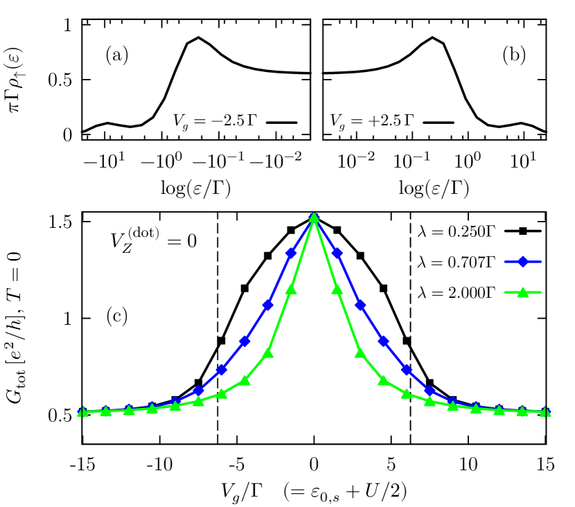
Figure 10: (Color online) Conductance effects of the detuning from particle–hole symmetry produced by a gate voltage $V_{g}$. For $|V_{Z}^{({\rm M})}|\lesssim T_{K}$, the spin–up DOS at the Fermi level drops as the Kondo peak is shifted to positive (negative) values for $V_{g}>0$ ($V_{g}<0$), due to the Majorana–induced Zeeman splitting $V_{Z}^{(\text{M})}$. This is shown in panels (a) and (b), respectively. The Kondo effect finally disappears for $|V_{g}|\gtrsim U/2$ due to the charge fluctuations of the mixed–valence regime. The conductance effects of the Kondo quench are shown in panel (c). The enhanced conductance at zero detuning ($V_{g}=0$) comes from both the “0.5” and the Kondo peaks, whereas after the suppression of the Kondo effect the persistent $0.5\,G_{0}$ conductance comes only from the “0.5” peak. Parameters: $\varepsilon_{\text{dot}}=-U/2=-6.25\,\Gamma$; $V_{Z}^{(\text{dot})}=0$.

While establishing such a specific value in a transport experiment is far from trivial, a much simpler test for the presence of the Majorana mode can be carried out by quenching the Kondo effect using gate voltages or magnetic fields. A conductance drop will be observed as the Kondo resonance disappears but the conductance signature of $G=0.5\,G_{0}$ from the Majorana mode remains. The ratio of the conductance before and after the Kondo quench can be used as an indicator of the Majorana physics.

The Kondo effect occurs when the QD is close to particle–hole symmetry. When the QD level is detuned from the symmetric point by a gate voltage $V_{g}$, an effective Zeeman splitting arises from the spin–symmetry breaking induced by the Majorana mode, which couples exclusively to the spin–down degree of freedom. For a small gate voltage $V_{g}\ll|\varepsilon_{\text{dot}}|$ this splitting is given to first order in $V_{g}$ asLee et al. (2013)

$$V_{Z}^{(\text{M})}=V_{g}\frac{8\lambda^{2}}{U^{2}}.$$ (24)

In terms of the minimal effective model, this field appears because only the spin–down electron of the dot is coupled to the Majorana mode. This spin asymmetry is explicitly introduced in the underlying microscopic tight–binding model by the magnetic field in the nanowire. Virtual processes involving the Majorana mode, the QD, and the band electrons lower the energy of the spin–down level through holelike excitations and that of the spin–up level indirectly through particle–like excitations. Thus, within the low–energy effective model, the Majorana mode gives rise to a Zeeman splitting within the QD when the dot is not particle–hole symmetric ($\varepsilon_{0,s}\neq-U/2$).

The effective Zeeman splitting (24) has an important effect on the spin–up spectral density shown in Figs. 10(a) and 10(b) for $|V_{Z}^{(\text{M})}|\lesssim T_{K}$. As this Zeeman splitting increases, the amplitude of the spin–up density of states at the Fermi level is reduced, and the Kondo effect is quenched; this reduces the low–temperature conductance, as shown in Fig. 10(c). In contrast and more importantly, the $0.5$ peak of the spin–down density of states remains pinned at the Fermi level (not shown). For $\lambda=2\,\Gamma$ (triangles) the effective Zeeman splitting $V_{Z}^{(\text{M})}$ strongly suppresses the Kondo effect, even for small $V_{g}$, well within the single–occupancy regime. In the case of $\lambda=0.25\,\Gamma$ the splitting $V_{Z}^{(\text{M})}$ is weaker, and the Kondo effect is ultimately quenched when the QD enters the mixed–valence regime—that is, when its charge begins fluctuating between single and double occupancy ($V_{g}\approx-U/2$) or between single and zero occupancy ($V_{g}\approx U/2$)—as indicated by the vertical dashed lines (see Appendix C). Note, however, that the spin–down contribution to the conductance is fixed at $0.5(\pi\Gamma)^{-1}$ for all values of $V_{g}$ due to the robustness of the “0.5” peak.

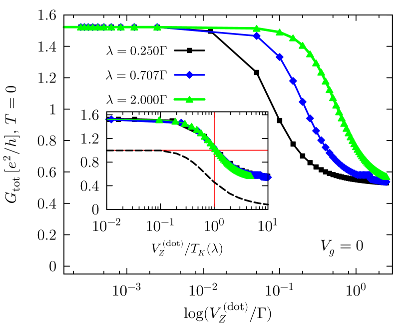
Figure 11: (Color online) Low–temperature zero–bias conductance of the QD as a function of the Zeeman splitting $V_{Z}^{(\text{dot})}$. Inset: Universality curve resulting from the rescaling $V_{Z}^{(\text{dot})}/T_{K}(\lambda)$. $T_{K}(\lambda)$ was obtained from Fig. 9. The dashed curve corresponds to the spin–up conductance for $\lambda=0$, and is given as a reference. Parameters: $\varepsilon_{\text{dot}}=-U/2=-6.25\,\Gamma$.

Perhaps more illuminating are the effects of an induced magnetic field, which breaks the spin degeneracy that is indispensable for the formation of the Kondo ground state. A Zeeman field of strength $V_{Z}^{(\text{dot})}\gtrsim T_{K}$ will suppress the Kondo zero–bias peak, and hence reduce the low–temperature conductance. This conductance suppression follows a well–known universality curve when the Zeeman splitting is rescaled by the Kondo temperature.Hewson (1993); Costi (2000) This is shown in Fig. 11, where three different values of the coupling $\lambda$ are considered. The same behavior is observed for all three cases: a conductance plateau of $G=1.5\,G_{0}$ for $V_{Z}^{(\text{dot})}\ll T_{K}$, followed by a monotonic decrease with $V_{Z}^{(\text{dot})}$ until reaching another plateau of $G=0.5\,G_{0}$ when $V_{Z}^{(\text{dot})}\gg T_{K}$, due solely to the Majorana mode. Moreover, the conductance versus $V_{Z}^{(\text{dot})}$ curve for a Kondo QD is known to be universal.Logan and Dickens (2001) The three curves in Fig. 11 collapse onto a single universal curve by rescaling the Zeeman splitting in terms of the Kondo temperature $T_{K}(\lambda)$ corresponding to each value of $\lambda$, which we obtained from Fig. 9. The experimental observation of this curve provides certainty that the Kondo effect was present in the QD, and that the applied magnetic field has eliminated it from the picture, leaving only the Majorana zero–bias peak.

All of the results presented in this section can be measured experimentally and may provide a method for detecting the emergence of the Majorana zero mode at the end of the topological quantum wire. When the QD is near its particle–hole symmetric point and the Kondo signature mixes with the Majorana peak, a finite zero–bias conductance can be measured. The Kondo effect can then be removed with the introduction of a gate–compensated magnetic field, leaving a finite zero–bias conductance coming from the “0.5” Majorana peak. The “1.5 to 0.5” ratio of the initial and final conductances is a clear sign of Majorana physics. The Kondo quench can be verified from the universal behavior of the conductance as a function of the applied magnetic field.

We emphasize the importance of fixing the QD spin–down energy level by means of a gate voltage, since both relevant energy scales for transport in the QD, $T_{K}$ and $T_{M}$, are strongly dependent on its value. It is also important that these experiments be carried out at a sufficiently low temperature, $T\ll T_{K},\,T_{M}$. It is desirable that the Majorana energy scale be of the order of the Kondo temperature ($T_{M}\sim T_{K}$), because in the case of $T_{M}\ll T_{K}$ it may be difficult to resolve the “0.5” dip in the Kondo resonance at the Fermi level from the conductance measurements, especially if it is somewhat broadened by thermal effects. Using the wire parameters from Sec. III.2, and with $\Gamma\sim 100\,\mu\text{eV}$, the Kondo and Majorana temperature scales are approximately $300\,\text{mK}$.

VIII Conclusions

We have studied the low–temperature transport properties of a hybrid QD–topological quantum wire system, using a model that explicitly includes Rashba spin–orbit coupling and induced $s$–wave superconductivity in the quantum wire, and the local Coulomb interaction within the QD. Using recursive Green’s function calculations, we showed that only one of the QD spin degrees of freedom couples to the Majorana zero mode emerging at the end of the wire, whereas the other fully decouples. This is signaled by a zero–bias peak in the spin–resolved conductance of the QD, which is robust to the application of arbitrarily large gate voltages and Zeeman fields.

Through numerical calculations, we show that the low-energy physics of this full model can be captured by a minimally coupled effective Hamiltonian for both a noninteracting and an interacting quantum dot. These models have been extensively used in the literature to describe the interaction between a quantum impurity and a Majorana fermion.

The effective model was investigated using the numerical renormalization group. We studied the interacting regime of the QD, where the Kondo effect appears and the mean–field Green’s function calculations are no longer valid. Our results show that the Majorana signature persists and suggest a QD ground state where Majorana and Kondo physics coexist.

Finally, we proposed a method for identifying the interplay between Majorana and Kondo physics in the system. The QD zero–bias conductance should be measured close to particle–hole symmetry, where the Majorana and the Kondo physics coexist; this value is taken as a reference. The Kondo effect should be quenched by a Zeeman field in the QD, and the field–dependent conductance measured. For a large Zeeman splitting the conductance will be determined by the “0.5” peak, giving a value of $0.5\,e^{2}/h$—a third of the reference conductance—corresponding only to the Majorana signature. The quenching of the Kondo effect can be verified from the universality properties of the conductance versus Zeeman field curves.

Appendix A Iterative equations for the Green’s function of the quantum wire

We make use of the spectral representation of the retarded Green’s functionZubarev (1960)

$$\langle\langle A;\,B\rangle\rangle_{\varepsilon}\equiv-i\int e^{i\varepsilon\tau}\Theta(\tau)\langle\left[A(\tau),\,B(0)\right]_{+}\rangle d\tau,$$ (25)

where $A(\tau)$ and $B(\tau)$ are the operators $A$ and $B$ in the Heisenberg picture, and $A$ and $B$ represent any combination of fermion operators in the Hamiltonian. The (anti–)commutator is written as $[A,\,B]_{\pm}=AB\pm BA$, and $\langle\cdots\rangle$ is the thermodynamic average at finite temperature, or the ground–state expectation value in the case of zero temperature. From the standard equation of motion technique we have the recursion relationZubarev (1960)

$$\varepsilon\langle\langle A;\,B\rangle\rangle_{\varepsilon}=\langle\left[A,\,B\right]_{+}\rangle+\langle\langle\left[A,\,H\right]_{-};\,B\rangle\rangle_{\varepsilon}.$$ (26)

In order to show how we obtained the iterative procedure in a pedagogical fashion, let us start by calculating the local Green’s function for the site $N-1$. We assume for the time being that the wire has only two other sites: the sites $N-2$ and $N$. This will allow us to see how the structure of the iterative procedure for arbitrary $N$ emerges. Given that we are ultimately interested in the local density of states

$$\rho_{j,s}(\varepsilon)=-\frac{1}{\pi}{\rm Im}\langle\langle c_{j,s};\,c^{\dagger}_{j,s}\rangle\rangle_{\varepsilon},$$ (27)

we will start by calculating the Green’s function $\langle\langle c_{j,s};\,c_{j,s}\rangle\rangle_{\varepsilon}$. Using Eq. (26) we can write the expressions for $\langle\langle c_{j,\uparrow};\,c_{j,s^{\prime}}\rangle\rangle_{\varepsilon}$ and $\langle\langle c_{j,\downarrow};\,c_{j,s^{\prime}}\rangle\rangle_{\varepsilon}$ as

$$\begin{split}&(\varepsilon-\varepsilon_{N-1,\uparrow})\langle\langle c_{N-1,\uparrow};\,c^{\dagger}_{N-1,s^{\prime}}\rangle\rangle_{\varepsilon}\\ &\quad=\delta_{s^{\prime}\uparrow}-\frac{t}{2}\langle\langle c_{N,\uparrow};\,c^{\dagger}_{N-1,s^{\prime}}\rangle\rangle_{\varepsilon}+\Delta\langle\langle c^{\dagger}_{N-1,\downarrow};\,c^{\dagger}_{N-1,s^{\prime}}\rangle\rangle_{\varepsilon}\\ &\qquad-t_{\rm SO}\langle\langle c_{N,\downarrow};\,c^{\dagger}_{N-1,s^{\prime}}\rangle\rangle_{\varepsilon},\end{split}$$ (28)

and

$$\begin{split}&(\varepsilon-\varepsilon_{N-1,\downarrow})\langle\langle c_{N-1,\downarrow};\,c^{\dagger}_{N-1,s^{\prime}}\rangle\rangle_{\varepsilon}\\ &\quad=\delta_{s^{\prime}\downarrow}-\frac{t}{2}\langle\langle c_{N,\downarrow};\,c^{\dagger}_{N-1,s^{\prime}}\rangle\rangle_{\varepsilon}-\Delta\langle\langle c^{\dagger}_{N-1,\uparrow};\,c^{\dagger}_{N-1,s^{\prime}}\rangle\rangle_{\varepsilon}\\ &\qquad+t_{\rm SO}\langle\langle c_{N,\uparrow};\,c^{\dagger}_{N-1,s^{\prime}}\rangle\rangle_{\varepsilon}.\end{split}$$ (29)

In Eqs. (28) and (29) we have defined $\varepsilon_{j,s}=-\mu+\sigma^{z}_{ss}V_{Z}$ in order to simplify the notation. The second term on the right–hand side of each equation describes simply the hopping between adjacent sites of the wire. The third term describes a hopping between adjacent sites, accompanied by a spin flip due to the Rashba spin–orbit coupling. Finally, the fourth term pairs electrons of opposite spin within a given site due to the $s$–wave superconductivity. We now need to calculate the equations of motion for these additional correlation functions. For instance, for the pairing correlation function we obtain

$$\begin{split}&(\varepsilon+\varepsilon_{N-1,\downarrow})\langle\langle c^{\dagger}_{N-1,\downarrow};\,c^{\dagger}_{N-1,s^{\prime}}\rangle\rangle_{\varepsilon}\\ &\quad=\Delta\langle\langle c_{N-1,\uparrow};\,c^{\dagger}_{N-1,s^{\prime}}\rangle\rangle_{\varepsilon}+\frac{t}{2}\langle\langle c^{\dagger}_{N,\downarrow};\,c^{\dagger}_{N-1,s^{\prime}}\rangle\rangle_{\varepsilon}\\ &\qquad-t_{\rm SO}\langle\langle c^{\dagger}_{N,\uparrow};\,c^{\dagger}_{N-1,s^{\prime}}\rangle\rangle_{\varepsilon},\end{split}$$ (30)

and

$$\begin{split}&(\varepsilon+\varepsilon_{N-1,\uparrow})\langle\langle c^{\dagger}_{N-1,\uparrow};\,c^{\dagger}_{N-1,s^{\prime}}\rangle\rangle_{\varepsilon}\\ &\quad=-\Delta\langle\langle c_{N-1,\downarrow};\,c^{\dagger}_{N-1,s^{\prime}}\rangle\rangle_{\varepsilon}+\frac{t}{2}\langle\langle c^{\dagger}_{N,\uparrow};\,c^{\dagger}_{N-1,s^{\prime}}\rangle\rangle_{\varepsilon}\\ &\qquad+t_{\rm SO}\langle\langle c^{\dagger}_{N,\downarrow};\,c^{\dagger}_{N-1,s^{\prime}}\rangle\rangle_{\varepsilon}.\end{split}$$ (31)

From the structure of the equations above it becomes clear that we can define a matrix for each chain site, which contains all of the correlation functions at that site:

$$\begin{split}&{\bf G}_{i,j}(\varepsilon)=\\ &\begin{pmatrix}\langle\langle c_{i,\uparrow};\,c^{\dagger}_{j,\uparrow}\rangle\rangle_{\varepsilon}&\langle\langle c_{i,\uparrow};\,c_{j,\downarrow}^{\dagger}\rangle\rangle_{\varepsilon}&\langle\langle c_{i,\uparrow};\,c_{j,\uparrow}\rangle\rangle_{\varepsilon}&\langle\langle c_{i,\uparrow};\,c_{j,\downarrow}\rangle\rangle_{\varepsilon}\\ \langle\langle c_{i,\downarrow};\,c^{\dagger}_{j,\uparrow}\rangle\rangle_{\varepsilon}&\langle\langle c_{i,\downarrow};\,c^{\dagger}_{j,\downarrow}\rangle\rangle_{\varepsilon}&\langle\langle c_{i,\downarrow};\,c_{j,\uparrow}\rangle\rangle_{\varepsilon}&\langle\langle c_{i,\downarrow};\,c_{j,\downarrow}\rangle\rangle_{\varepsilon}\\ \langle\langle c_{i,\uparrow}^{\dagger};\,c^{\dagger}_{j,\uparrow}\rangle\rangle_{\varepsilon}&\langle\langle c_{i,\uparrow}^{\dagger};\,c_{j,\downarrow}^{\dagger}\rangle\rangle_{\varepsilon}&\langle\langle c_{i,\uparrow}^{\dagger};\,c_{j,\uparrow}\rangle\rangle_{\varepsilon}&\langle\langle c^{\dagger}_{i,\uparrow};\,c_{j,\downarrow}\rangle\rangle_{\varepsilon}\\ \langle\langle c^{\dagger}_{i,\downarrow};\,c^{\dagger}_{j,\uparrow}\rangle\rangle_{\varepsilon}&\langle\langle c^{\dagger}_{i,\downarrow};\,c^{\dagger}_{j,\downarrow}\rangle\rangle_{\varepsilon}&\langle\langle c^{\dagger}_{i,\downarrow};\,c_{j,\uparrow}\rangle\rangle_{\varepsilon}&\langle\langle c^{\dagger}_{i,\downarrow};\,c_{j,\downarrow}\rangle\rangle_{\varepsilon}\end{pmatrix}.\end{split}$$ (32)

With this notation, the system of equations can be written as

$$\begin{split}{\bf G}_{N-1,N-1}(\varepsilon)=&\,\,{\bf g}_{N-1,N-1}(\varepsilon)\\ &+{\bf g}_{N-1,N-1}(\varepsilon){\bf V}{\bf G}_{N-1,N-1}(\varepsilon)\\ &+{\bf g}_{N-1,N-1}(\varepsilon){\bf t}{\bf G}_{N,N-1}(\varepsilon),\end{split}$$ (33)

where we have defined the bare local Green’s function for a generic site,

$${\bf g}_{j,j}(\varepsilon)=\begin{pmatrix}\frac{1}{\varepsilon-\varepsilon_{\uparrow}}&0&0&0\\ 0&\frac{1}{\varepsilon-\varepsilon_{\downarrow}}&0&0\\ 0&0&\frac{1}{\varepsilon+\varepsilon_{\uparrow}}&0\\ 0&0&0&\frac{1}{\varepsilon+\varepsilon_{\downarrow}}\end{pmatrix},$$ (34)

and the matrices

$${\bf V}=\begin{pmatrix}0&0&0&\Delta\\ 0&0&-\Delta&0\\ 0&-\Delta&0&0\\ \Delta&0&0&0\end{pmatrix},$$ (35a)

$${\bf t}=\begin{pmatrix}\frac{-t}{2}&-t_{\rm SO}&0&0\\ -t_{\rm SO}&\frac{-t}{2}&0&0\\ 0&0&\frac{-t}{2}&t_{\rm SO}\\ 0&0&-t_{\rm SO}&\frac{-t}{2}\end{pmatrix},$$ (35b)

which, respectively, pair the electrons in each site of the chain and allow for the electrons to hop between adjacent sites, either preserving the spin projection or flipping it. Moreover, we can write Eq. (33) in the more compact Dyson equation form

$$\begin{split}{\bf G}_{N-1,N-1}(\varepsilon)=&\,\tilde{\bf g}_{N-1,N-1}(\varepsilon)\\ &+\tilde{\bf g}_{N-1,N-1}(\varepsilon){\bf t}{\bf G}_{N,N-1}(\varepsilon),\end{split}$$ (36)

with the definition

$$\tilde{\bf g}_{j,j}(\varepsilon)=(1-{\bf V})^{-1}{\bf g}_{j,j}(\varepsilon).$$ (37)

Repeating these steps for the nonlocal Green’s function ${\bf G}_{N,N-1}(\varepsilon)$, we obtain

$${\bf G}_{N,N-1}(\varepsilon)=\tilde{\bf g}_{N,N}(\varepsilon)\hat{\bf t}^{\dagger}{\bf G}_{N-1,N-1}(\varepsilon).$$ (38)

Finally, substituting Eq. (38) into (36) we find

$$\begin{split}{\bf G}_{N-1,N-1}(\varepsilon)=&\left[1-\tilde{\bf g}_{N-1,N-1}(\varepsilon){\bf t}\tilde{\bf g}_{N,N}(\varepsilon){\bf t}^{\dagger}\right]^{-1}\\ &\times\tilde{\bf g}_{N-1,N-1}(\varepsilon).\end{split}$$ (39)

Equation (39) establishes the iterative procedure, in which for site $N-1$ we simply replace $\tilde{\bf g}_{N-1,N-1}(\varepsilon)$ by ${\bf G}_{N-1,N-1}(\varepsilon)$, which was calculated in the very first iteration. This procedure can be repeated $N$ times in order to obtain the full numerical Green’s function at one end of the wire. For very large $N$, ${\bf G}_{1,1}(\varepsilon)$ will be indistinguishable from ${\bf G}_{2,2}(\varepsilon)$; at that point the semi-infinite chain limit will have been reached.

Appendix B The Green’s function of the quantum dot

For the derivation of the local Green’s function of the QD, we assume that the QD is symmetrically coupled to the right and left terminals and replace them by a symmetrized band with a coupling $\tilde{V}_{\mathbf{k}}=\sqrt{2}V_{\ell\mathbf{k}}$. The total hybridization function for the symmetric band is given by $\Gamma(\omega)=\pi\sum_{\mathbf{k}}\,|\tilde{V}_{\mathbf{k}}|^{2}\delta(\omega-\varepsilon_{\mathbf{k}})$, with $\varepsilon_{\mathbf{k}}$ the band dispersion. The complementary asymmetric band, on the other hand, is decoupled from the QD, and contributes only a constant energy to the Hamiltonian which can be neglected.

The local Green’s function at the QD site is given by the equation of motion

$$\langle\langle c_{0,s};\,c_{0,s^{\prime}}^{\dagger}\rangle\rangle_{\varepsilon}=\delta_{ss^{\prime}}+\langle\langle\left[c_{0,s},\,H\right]_{-};\,c_{0,s^{\prime}}^{\dagger}\rangle\rangle_{\varepsilon}.$$ (40)

Evaluating the commutator

$$\begin{split}\left[c_{0,s},\,H\right]_{-}=&\varepsilon_{0,s}c_{0,s}+U\,n_{0,\bar{s}}c_{0,s}\\ &-t_{0}c_{1,s}+\sum_{\mathbf{k}}\tilde{V}_{\mathbf{k}}c_{\mathbf{k},s},\end{split}$$ (41)

we obtain

$$\begin{split}&\left(\varepsilon-\varepsilon_{0,s}\right)\langle\langle c_{0,s};\,c_{0,s^{\prime}}^{\dagger}\rangle\rangle_{\varepsilon}=\delta_{ss^{\prime}}+U\langle\langle n_{0,\bar{s}}c_{0,s};\,c_{0,s^{\prime}}^{\dagger}\rangle\rangle_{\varepsilon}\\ &-t_{0}\langle\langle c_{1,s};\,c_{0,s^{\prime}}^{\dagger}\rangle\rangle_{\varepsilon}-\sum_{\mathbf{k}}\tilde{V}_{\mathbf{k}}\langle\langle c_{\mathbf{k},s};\,c_{0,s^{\prime}}^{\dagger}\rangle\rangle_{\varepsilon}.\end{split}$$ (42)

The three new correlation functions on the right–hand side must be evaluated as well. The first and last obey the equation of motion

$$\begin{split}&\left(\varepsilon-\varepsilon_{0,s}-U\right)\langle\langle n_{0,\bar{s}}c_{0,s};\,c_{0,s^{\prime}}^{\dagger}\rangle\rangle_{\varepsilon}=\langle n_{0,\bar{s}}\rangle\delta_{ss\prime}+\langle c^{\dagger}_{0,\bar{s}}c_{0,s}\rangle\delta_{s^{\prime},\bar{s}}+\sum_{\mathbf{k}}\tilde{V}_{\mathbf{k}}\langle\langle n_{0,\bar{s}}c_{\mathbf{k},s};\,c^{\dagger}_{0,s^{\prime}}\rangle\rangle_{\varepsilon}+\sum_{\mathbf{k}}\tilde{V}_{\mathbf{k}}\langle\langle c^{\dagger}_{0,\bar{s}}c_{\mathbf{k},\bar{s}}c_{0,s};\,c^{\dagger}_{0,s^{\prime}}\rangle\rangle_{\varepsilon}\\ &-\sum_{\mathbf{k}}\tilde{V}^{*}_{\mathbf{k}}\langle\langle c^{\dagger}_{\mathbf{k},\bar{s}}c_{0,\bar{s}}c_{0,s};\,c^{\dagger}_{0,s^{\prime}}\rangle\rangle_{\varepsilon}-t_{0}\langle\langle n_{0,\bar{s}}c_{1,s};\,c^{\dagger}_{0,s^{\prime}}\rangle\rangle_{\varepsilon}-t_{0}\langle\langle c^{\dagger}_{0,\bar{s}}c_{1,\bar{s}}c_{0,s};\,c^{\dagger}_{0,s^{\prime}}\rangle\rangle_{\varepsilon}+t_{0}\langle\langle c^{\dagger}_{1,\bar{s}}c_{0,\bar{s}}c_{0,s};\,c^{\dagger}_{0,s^{\prime}}\rangle\rangle_{\varepsilon}.\end{split}$$ (43)

At this point we use the Hubbard I decoupling procedure, introducing the following approximations:

$$\langle\langle n_{0,\bar{s}}c_{1,s};\,c^{\dagger}_{0,s^{\prime}}\rangle\rangle_{\varepsilon}\approx\langle n_{0,\bar{s}}\rangle\langle\langle c_{1,s};\,c^{\dagger}_{0,s^{\prime}}\rangle\rangle_{\varepsilon},$$ (44a)

$$\begin{split}&\sum_{\mathbf{k}}\tilde{V}_{\mathbf{k}}\langle\langle n_{0,\bar{s}}c_{\mathbf{k},s};\,c^{\dagger}_{0,s^{\prime}}\rangle\rangle_{\varepsilon}\\ &\quad\approx\langle n_{0,\bar{s}}\rangle\sum_{\mathbf{k}}\tilde{V}_{\mathbf{k}}\langle\langle n_{0,\bar{s}}c_{\mathbf{k},s};\,c^{\dagger}_{0,s^{\prime}}\rangle\rangle_{\varepsilon},\end{split}$$ (44b)

$$\begin{split}&\sum_{\mathbf{k}}\tilde{V}_{\mathbf{k}}\langle\langle c^{\dagger}_{0,\bar{s}}c_{\mathbf{k},\bar{s}}c_{0,s};\,c^{\dagger}_{0,s^{\prime}}\rangle\rangle_{\varepsilon}\\ &\quad\approx\sum_{\mathbf{k}}\tilde{V}_{\mathbf{k}}\langle c^{\dagger}_{0,\bar{s}}c_{\mathbf{k},\bar{s}}\rangle\langle\langle c_{0,s};\,c^{\dagger}_{0,s^{\prime}}\rangle\rangle_{\varepsilon},\end{split}$$ (44c)

$$\begin{split}&\sum_{\mathbf{k}}\tilde{V}^{*}_{\mathbf{k}}\langle\langle c^{\dagger}_{\mathbf{k},\bar{s}}c_{0,\bar{s}}c_{0,s};\,c^{\dagger}_{0,s^{\prime}}\rangle\rangle_{\varepsilon}\\ &\quad\approx\sum_{\mathbf{k}}\tilde{V}^{*}_{\mathbf{k}}\langle c^{\dagger}_{\mathbf{k},\bar{s}}c_{0,\bar{s}}\rangle\langle\langle c_{0,s};\,c^{\dagger}_{0,s^{\prime}}\rangle\rangle_{\varepsilon},\end{split}$$ (44d)

$$\langle\langle c^{\dagger}_{0,\bar{s}}c_{1,\bar{s}}c_{0,s};\,c^{\dagger}_{0,s^{\prime}}\rangle\rangle_{\varepsilon}\approx\langle c^{\dagger}_{0,\bar{s}}c_{1,\bar{s}}\rangle\langle\langle c_{0,s};\,c^{\dagger}_{0,s^{\prime}}\rangle\rangle_{\varepsilon},$$ (44e)

$$\langle\langle c^{\dagger}_{1,\bar{s}}c_{0,\bar{s}}c_{0,s};\,c^{\dagger}_{0,s^{\prime}}\rangle\rangle_{\varepsilon}\approx\langle c^{\dagger}_{1,\bar{s}}c_{0,\bar{s}}\rangle\langle\langle c_{0,s};\,c^{\dagger}_{0,s^{\prime}}\rangle\rangle_{\varepsilon}.$$ (44f)

Moreover, we assume that $\sum_{\mathbf{k}}\tilde{V}^{*}_{\mathbf{k}}\langle c^{\dagger}_{\mathbf{k},\bar{s}}c_{0,\bar{s}}\rangle\!=\!\sum_{\mathbf{k}}\tilde{V}_{\mathbf{k}}\langle c^{\dagger}_{0,\bar{s}}c_{\mathbf{k},\bar{s}}\rangle$, and that $\langle c^{\dagger}_{0,\bar{s}}c_{1,\bar{s}}\rangle\!=\!\langle c^{\dagger}_{1,\bar{s}}c_{0,\bar{s}}\rangle$. With these assumptions we get

$$\begin{split}&\left(\varepsilon-\varepsilon_{0,s}-U\right)\langle\langle n_{0,\bar{s}}c_{0,s};\,c_{0,s^{\prime}}^{\dagger}\rangle\rangle_{\varepsilon}=\\ &\quad\langle n_{0,\bar{s}}\rangle\delta_{ss^{\prime}}+\langle c^{\dagger}_{0,\bar{s}}c_{0,s}\rangle\delta_{s^{\prime},\bar{s}}+\langle n_{0,\bar{s}}\rangle\sum_{\mathbf{k}}\tilde{V}_{\mathbf{k}}\langle\langle c_{\mathbf{k},s};\,c^{\dagger}_{0,s^{\prime}}\rangle\rangle_{\varepsilon}\\ &\quad-t_{0}\langle n_{0,\bar{s}}\rangle\langle\langle c_{1,s};\,c^{\dagger}_{0,s^{\prime}}\rangle\rangle_{\varepsilon}.\end{split}$$ (45)

It is now straightforward to obtain the following expression for $\langle\langle c_{\mathbf{k},s};\,c^{\dagger}_{0,s^{\prime}}\rangle\rangle_{\varepsilon}$:

$$\langle\langle c_{\mathbf{k},s};\,c^{\dagger}_{0,s^{\prime}}\rangle\rangle_{\varepsilon}=-\frac{\tilde{V}_{\mathbf{k}}^{*}}{\varepsilon-\varepsilon_{\mathbf{k}}}\langle\langle c_{0,s};\,c^{\dagger}_{0,s^{\prime}}\rangle\rangle_{\varepsilon}.$$ (46)

Substituting Eq. (46) into Eq. (45), and then the resulting expression into (42), we obtain

$$\begin{split}\left[\varepsilon-\varepsilon_{0,s}-\left(1+\frac{U\langle n_{0,\bar{s}}\rangle}{\varepsilon-\varepsilon_{0,s}-U}\right)\sum_{\mathbf{k}}\frac{|\tilde{V}_{\mathbf{k}}|^{2}}{\varepsilon-\varepsilon_{\mathbf{k}}}\right]\langle\langle c_{0,s};\,c_{0,s^{\prime}}^{\dagger}\rangle\rangle_{\varepsilon}=&\,\,\delta_{ss^{\prime}}+\frac{U\langle n_{0,\bar{s}}\rangle\delta_{ss^{\prime}}+U\langle c^{\dagger}_{0,\bar{s}}c_{0,s}\rangle\delta_{\bar{s}s^{\prime}}}{\varepsilon-\varepsilon_{0,s}-U}\\ &-\left(1+\frac{U\langle n_{0,\bar{s}}\rangle}{\varepsilon-\varepsilon_{0,s}-U}\right)t_{0}\langle\langle c_{1,s};\,c^{\dagger}_{0,s^{\prime}}\rangle\rangle_{\varepsilon}.\end{split}$$ (47)

The expression above is simplified in the wide–band limit for the electronic band, in which case $\sum_{\mathbf{k}}|\tilde{V}_{\mathbf{k}}|^{2}/(\varepsilon-\varepsilon_{\mathbf{k}})=-i\,\Gamma(\varepsilon)$. We can simplify this even further by assuming a “flat” density of states, so that $\Gamma(\varepsilon)\equiv\Gamma$ is a constant.

Some algebraic manipulation leads to the compact form

$$\begin{split}\langle\langle c_{0,s};\,c_{0,s^{\prime}}^{\dagger}\rangle\rangle_{\varepsilon}=&\,\tilde{g}_{0s,0s}(\varepsilon)\delta_{ss^{\prime}}+\frac{A_{g,s}(\varepsilon)U\langle c^{\dagger}_{0,\bar{s}}c_{0,s}\rangle\delta_{\bar{s}s^{\prime}}}{(\varepsilon-\varepsilon_{0,s})(\varepsilon-\varepsilon_{0,s}-U)}\\ &-\tilde{g}_{0s,0s}(\varepsilon)t_{0}\langle\langle c_{1,s};\,c^{\dagger}_{0,s^{\prime}}\rangle\rangle_{\varepsilon},\end{split}$$ (48)

with

$$A_{g,s}(\varepsilon)=\frac{1}{1+i\Gamma g_{0s,0s}(\varepsilon)},$$ (49)

and

$$g_{0s,0s}(\varepsilon)=\frac{1-\langle n_{0,\bar{s}}\rangle}{\varepsilon-\varepsilon_{0,s}}+\frac{\langle n_{0,\bar{s}}\rangle}{\varepsilon-\varepsilon_{0,s}-U}.$$ (50)

Eqution (50) is the exact Green’s function for the QD in the atomic limit ($\tilde{V}_{\mathbf{k}}=t_{0}=0$).

We now need to evaluate the Green’s function $\langle\langle c^{\dagger}_{0,s};\,c^{\dagger}_{0,s^{\prime}}\rangle\rangle_{\varepsilon}$. We have

$$\begin{split}\langle\langle c^{\dagger}_{0,s};\,c_{0,s^{\prime}}^{\dagger}\rangle\rangle_{\varepsilon}=&\,\frac{-A_{h,s}(\varepsilon)U\langle c^{\dagger}_{0,\bar{s}}c^{\dagger}_{0,s}\rangle\delta_{s^{\prime}\bar{s}}}{(\varepsilon+\varepsilon_{0,s})(\varepsilon+\varepsilon_{0,s}+U)}\\ &+\tilde{h}_{0s,0s}t_{0}\langle\langle c^{\dagger}_{1,s};\,c^{\dagger}_{0,s^{\prime}}\rangle\rangle_{\varepsilon},\end{split}$$ (51)

where

$$\tilde{h}_{0s,0s}(\varepsilon)=A_{h,s}(\varepsilon)h_{0s,0s}(\varepsilon),$$ (52)

$$A_{h,s}(\varepsilon)=\frac{1}{1+i\Gamma h_{0s,0s}(\varepsilon)},$$ (53)

and

$$h_{0s,0s}(\varepsilon)=\frac{1+\langle n_{0,\bar{s}}\rangle}{\varepsilon+\varepsilon_{0,s}}-\frac{\langle n_{0,\bar{s}}\rangle}{\varepsilon+\varepsilon_{0,s}+U}.$$ (54)

Finally, we can write the Green’s function for the QD in the limit of $t_{0}=0$, within the Hubbard I approximation, as

$${\bf g}_{0,0}(\varepsilon)=\begin{bmatrix}\tilde{g}_{0\uparrow,0\uparrow}(\varepsilon)&\frac{A_{g,\uparrow}(\varepsilon)U\langle c^{\dagger}_{0,\downarrow}c_{0,\uparrow}\rangle}{(\varepsilon-\varepsilon_{0,\uparrow})(\varepsilon-\varepsilon_{0,\uparrow}-U)}&0&\frac{A_{g,\uparrow}(\varepsilon)U\langle c_{0,\downarrow}c_{0,\uparrow}\rangle}{(\varepsilon-\varepsilon_{0,\uparrow})(\varepsilon-\varepsilon_{0,\uparrow}-U)}\\ \frac{A_{g,\downarrow}(\varepsilon)U\langle c^{\dagger}_{0,\uparrow}c_{0,\downarrow}\rangle}{(\varepsilon-\varepsilon_{0,\downarrow})(\varepsilon-\varepsilon_{0,\downarrow}-U)}&\tilde{g}_{0\downarrow,0\downarrow}(\varepsilon)&\frac{A_{g,\downarrow}(\varepsilon)U\langle c_{0,\uparrow}c_{0,\downarrow}\rangle}{(\varepsilon-\varepsilon_{0,\downarrow})(\varepsilon-\varepsilon_{0,\downarrow}-U)}&0\\ 0&\frac{A_{h,\uparrow}(\varepsilon)U\langle c^{\dagger}_{0,\uparrow}c^{\dagger}_{0,\downarrow}\rangle}{(\varepsilon+\varepsilon_{0,\uparrow})(\varepsilon+\varepsilon_{0,\uparrow}+U)}&\tilde{h}_{0\uparrow,0\uparrow}(\varepsilon)&\frac{A_{h,\uparrow}(\varepsilon)U\langle c_{0,\downarrow}c^{\dagger}_{0,\uparrow}\rangle}{(\varepsilon+\varepsilon_{0,\uparrow})(\varepsilon+\varepsilon_{0,\uparrow}+U)}\\ \frac{A_{h,\downarrow}(\varepsilon)U\langle c^{\dagger}_{0,\downarrow}c^{\dagger}_{0,\uparrow}\rangle}{(\varepsilon+\varepsilon_{0,\downarrow})(\varepsilon+\varepsilon_{0,\downarrow}+U)}&0&\frac{A_{h,\downarrow}(\varepsilon)U\langle c_{0,\uparrow}c^{\dagger}_{0,\downarrow}\rangle}{(\varepsilon+\varepsilon_{0,\downarrow})(\varepsilon+\varepsilon_{0,\downarrow}+U)}&\tilde{h}_{0\downarrow,0\downarrow}(\varepsilon)\end{bmatrix}.$$ (55)

The coupling of the QD with the first site of the wire is given by the matrix

$${\bf t}_{0}=\begin{pmatrix}-t_{0}&0&0&0\\ 0&-t_{0}&0&0\\ 0&0&t_{0}&0\\ 0&0&0&t_{0}\end{pmatrix}.$$ (56)

Note that the Green’s function matrix (55) depends on various expectation values. The two occupations $\langle n_{0,\uparrow}\rangle$ and $\langle n_{0,\downarrow}\rangle$, appearing in the diagonal elements of ${\bf g}_{0,0}(\varepsilon)$, are given at finite temperature by

$$\langle n_{0,\uparrow}\rangle=-\frac{1}{\pi}\int_{-\infty}^{\infty}\mathrm{d}\varepsilon\,f(\varepsilon,\,T){\rm Im}~{}[{\bf G}_{0,0}(\varepsilon)]_{1,1},$$ (57)

and

$$\langle n_{0,\downarrow}\rangle=-\frac{1}{\pi}\int_{-\infty}^{\infty}\mathrm{d}\varepsilon\,f(\varepsilon,\,T){\rm Im}~{}[{\bf G}_{0,0}(\varepsilon)]_{2,2},$$ (58)

where $f(\varepsilon,\,T)=\left[1+\exp\left(\varepsilon/T\right)\right]^{-1}$ is the Fermi function. There are eight other expectation values appearing in the off–diagonal terms of the matrix (55). However, due to the anticommutation relations between fermionic operators, only four of them are independent:

$$\begin{split}\langle c^{\dagger}_{0,\downarrow}c_{0,\uparrow}\rangle&=-\langle c_{0,\uparrow}c^{\dagger}_{0,\downarrow}\rangle\\ &=-\frac{1}{\pi}\int_{-\infty}^{\infty}\mathrm{d}\varepsilon\,f(\varepsilon,\,T){\rm Im}~{}[{\bf G}_{0,0}(\varepsilon)]_{1,2},\end{split}$$ (59a)

$$\begin{split}\langle c^{\dagger}_{0,\uparrow}c_{0,\downarrow}\rangle&=-\langle c_{0,\downarrow}c^{\dagger}_{0,\uparrow}\rangle\\ &=-\frac{1}{\pi}\int_{-\infty}^{\infty}\mathrm{d}\varepsilon\,f(\varepsilon,\,T){\rm Im}~{}[{\bf G}_{0,0}(\varepsilon)]_{2,1},\end{split}$$ (59b)

$$\begin{split}\langle c_{0,\downarrow}c_{0,\uparrow}\rangle&=-\langle c_{0,\uparrow}c_{0,\downarrow}\rangle\\ &=-\frac{1}{\pi}\int_{-\infty}^{\infty}\mathrm{d}\varepsilon\,f(\varepsilon,\,T){\rm Im}~{}[{\bf G}_{0,0}(\varepsilon)]_{1,4},\end{split}$$ (59c)

and

$$\begin{split}\langle c^{\dagger}_{0,\uparrow}c^{\dagger}_{0,\downarrow}\rangle&=-\langle c^{\dagger}_{0,\downarrow}c^{\dagger}_{0,\uparrow}\rangle\\ &=-\frac{1}{\pi}\int_{-\infty}^{\infty}\mathrm{d}\varepsilon\,f(\varepsilon,\,T){\rm Im}~{}[{\bf G}_{0,0}(\varepsilon)]_{4,1}.\end{split}$$ (59d)

These expectation values depend on the Green’s functions themselves, and thus have to be computed self–consistently.

Appendix C Charge and spin polarization of the gated quantum dot coupled to a Majorana mode

In this appendix we justify our interpretation of the results presented in Fig. 10, Sec. VII. Equation (24) gives the Majorana–induced effective Zeeman splitting $V_{Z}^{(M)}$ for a small detuning from particle–hole symmetry, $|V_{g}|\ll|\varepsilon_{\text{dot}}|$.

For large enough $\lambda$, a small $V_{g}$ will quench the Kondo effect by breaking the spin symmetry. For $\lambda=2\,\Gamma$ (triangles), Figure 12(a) shows a rapid change in charge for both positive and negative $V_{g}$. For $|V_{g}|$ as small as $2.5\,\Gamma$, Fig. 10(c) demonstrates that the conductance enhancement due to the Kondo effect has decreased as much as $50\%$, even though the system is far from the mixed–valence regime. The negative (positive) spin polarization of the QD for positive (negative) $V_{g}$ shown in Fig. 12(b) demonstrates it is a Zeeman splitting accompanying the level shift by the gate voltage that kills the Kondo effect.

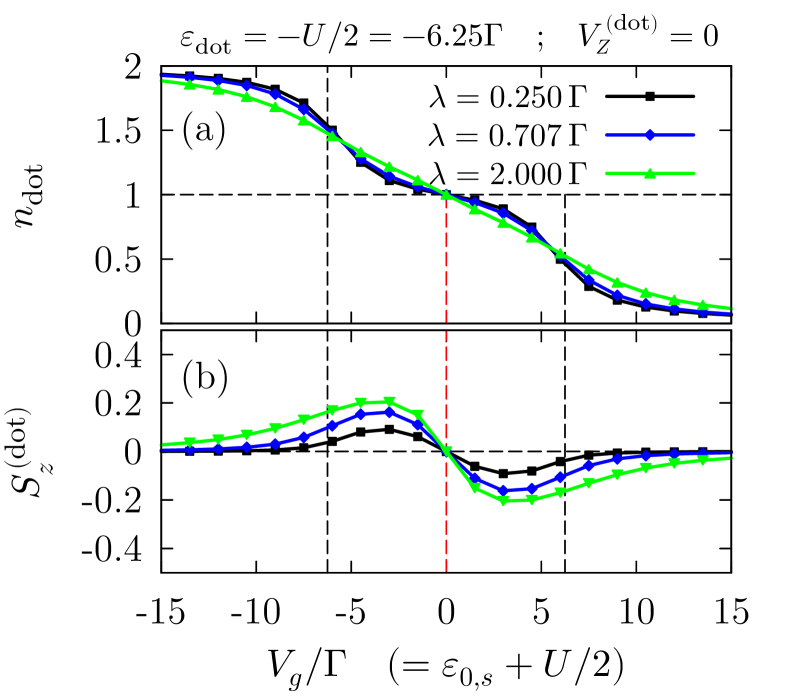
Figure 12: (Color online) Quantum dot occupancy (charge) and spin polarization for the parameters of Fig. 10.

On the other hand, for small enough $\lambda$ the Majorana–induced Zeeman splitting may be weak enough for the Kondo effect to survive until the mixed valence regime is reached, at which point it is quenched by charge fluctuations within the QD. For $\lambda=0.25\,\Gamma$ (squares), Fig. 10(c) shows a much slower decay of the enhanced conductance, where only for $|V_{g}|\sim|\varepsilon_{\text{dot}}|$ has the conductance contribution from the Kondo effect been reduced by half. At this point, indicated in Fig. 12 by the lateral vertical dashed lines, Fig. 12(a) shows that the QD is far away from single occupancy, this time with a negligible spin polarization presented in Fig. 12(b). This is clear indication that the mixed–valence regime has been reached, and the Kondo effect finally disappears due to charge fluctuations in the QD.

References

- Alicea (2012) J. Alicea, Reports on Progress in Physics 75, 076501 (2012).
- Kitaev (2001) A. Y. Kitaev, Phys.-Usp. 44, 131 (2001).
- Mourik et al. (2012) V. Mourik, K. Zuo, S. M. Frolov, S. R. Plissard, E. P. A. M. Bakkers, and L. P. Kouwenhoven, Science 336, 1003 (2012).
- Deng et al. (2012) M. T. Deng, C. L. Yu, G. Y. Huang, M. Larsson, P. Caroff, and H. Q. Xu, Nano Letters 12, 6414 (2012).
- Anindya Dasand Ronen et al. (2012) Y. Anindya Dasand Ronen, Y. Most, Y. Oreg, M. Heiblum, and H. Shtrikman, Nature Physics 8, 887 (2012).
- Lee et al. (2012) E. J. H. Lee, X. Jiang, R. Aguado, G. Katsaros, C. M. Lieber, and S. De Franceschi, Phys. Rev. Lett. 109, 186802 (2012).
- Churchill et al. (2013) H. O. H. Churchill, V. Fatemi, K. Grove-Rasmussen, M. T. Deng, P. Caroff, H. Q. Xu, and C. M. Marcus, Phys. Rev. B 87, 241401 (2013).
- Prada et al. (2012) E. Prada, P. San-Jose, and R. Aguado, Phys. Rev. B 86, 180503 (2012).
- Rainis et al. (2013) D. Rainis, L. Trifunovic, J. Klinovaja, and D. Loss, Phys. Rev. B 87, 024515 (2013).
- Cook et al. (2012) A. M. Cook, M. M. Vazifeh, and M. Franz, Phys. Rev. B 86, 155431 (2012).
- Liu and Lobos (2013) X.-J. Liu and A. M. Lobos, Phys. Rev. B 87, 060504 (2013).
- Stanescu et al. (2011) T. D. Stanescu, R. M. Lutchyn, and S. Das Sarma, Phys. Rev. B 84, 144522 (2011).
- Lee et al. (2014) E. J. H. Lee, X. Jiang, M. Houzet, R. Aguado, C. M. Lieber, and S. De Franceschi, Nature Nanotechnology 9, 79–84 (2014).
- Franz (2013) M. Franz, Nat. Nano. 8, 149 (2013).
- Nadj-Perge et al. (2013) S. Nadj-Perge, I. K. Drozdov, B. A. Bernevig, and A. Yazdani, Phys. Rev. B 88, 020407 (2013).
- Pientka et al. (2013) F. Pientka, L. I. Glazman, and F. von Oppen, Phys. Rev. B 88, 155420 (2013).
- Klinovaja et al. (2013) J. Klinovaja, P. Stano, A. Yazdani, and D. Loss, Phys. Rev. Lett. 111, 186805 (2013).
- Braunecker and Simon (2013) B. Braunecker and P. Simon, Phys. Rev. Lett. 111, 147202 (2013).
- Vazifeh and Franz (2013) M. M. Vazifeh and M. Franz, Phys. Rev. Lett. 111, 206802 (2013).
- Nakosai et al. (2013) S. Nakosai, Y. Tanaka, and N. Nagaosa, Phys. Rev. B 88, 180503 (2013).
- Fu and Kane (2008) L. Fu and C. L. Kane, Phys. Rev. Lett. 100, 096407 (2008).
- Alicea (2010) J. Alicea, Phys. Rev. B 81, 125318 (2010).
- Chung et al. (2011) S. B. Chung, H.-J. Zhang, X.-L. Qi, and S.-C. Zhang, Phys. Rev. B 84, 060510 (2011).
- Das Sarma et al. (2012) S. Das Sarma, J. D. Sau, and T. D. Stanescu, Phys. Rev. B 86, 220506 (2012).
- Nadj-Perge et al. (2014) S. Nadj-Perge, I. K. Drozdov, J. Li, H. Chen, S. Jeon, J. Seo, A. H. MacDonald, B. A. Bernevig, and A. Yazdani, Science 346, 602 (2014).
- Dumitrescu et al. (2015) Eugene Dumitrescu, Brenden Roberts, Sumanta Tewari, Jay D. Sau, S. Das Sarma, Phys. Rev. B 91, 094505 (2015).
- Liu and Baranger (2011) D. E. Liu and H. U. Baranger, Phys. Rev. B 84, 201308 (2011).
- Vernek et al. (2014) E. Vernek, P. H. Penteado, A. C. Seridonio, and J. C. Egues, Phys. Rev. B 89, 165314 (2014).
- (29) A. Golub, I. Kuzmenko, and Y. Avishai, Phys. Rev. Lett. 107, 176802 (2011).
- Lee et al. (2013) M. Lee, J. S. Lim, and R. López, Phys. Rev. B 87, 241402 (2013).
- Liu et al. (2015) Dong E. Liu, Meng Cheng, Roman M. Lutchyn, Phys. Rev. B 91, 081405 (2015).
- Chirla et al. (2014) R. Chirla, I. V. Dinu, V. Moldoveanu, and C. P. Moca, Phys. Rev. B 90, 195108 (2014).
- Cheng et al. (2014) M. Cheng, M. Becker, B. Bauer, and R. M. Lutchyn, Phys. Rev. X 4, 031051 (2014).
- (34) The systems discussed in Refs. Liu et al., 2015 and Lee et al., 2013 consist of a quantum dot coupled to a single lead, whereas Refs. Chirla et al., 2014 and Cheng et al., 2014 study a dot coupled to two leads, a source and a drain. However, in the case of identical source and drain leads, the system can be mapped onto a single lead setup through an appropriate rotation of their electron operators.
- Hubbard (1963) J. Hubbard, Proc. Roy. Soc. (London) A276, 238 (1963).
- Lacroix (1981) C. Lacroix, J. Phys. F: Metal Phys. 11, 2389 (1981).
- Flensberg (2010) K. Flensberg, Phys. Rev. B 82, 180516 (2010).
- de Sousa and Das Sarma (2003) R. de Sousa and S. Das Sarma, Phys. Rev. B 68, 155330 (2003).
- Potter and Lee (2011) A. C. Potter and P. A. Lee, Phys. Rev. B 83, 094525 (2011).
- (40) For a spatially varying see, for instance, Y. Oreg, G. Refel, and F. von Oppen, Phys. Rev. Lett. 105, 177002 (2010). See also some general discussions on the proximity effect by O. T. Valls, M. Bryan, and I. Žutić, Phys. Rev. B 82, 134534 (2010) and references therein.
- Zubarev (1960) D. N. Zubarev, Sov. Phys. Usp. 3, 320 (1960).
- Note (1) The results of Fig. 2(c) were correctly reproduced by the effective model Eq. (16), with an appropriate choice of . This indicates that the apparent delayed transition and the appearance of a suppressed and shifted central peak are not related to the wire degrees of freedom. Then, we considered the same parameters of the figure, except with a small Zeeman splitting in the dot , which quenches the Kondo effect (see Fig. 11) while keeping the system in a Coulomb blockade (). We also found the appropriate value of for this case to reproduce the results of the full model, and used it for NRG calculations. This allowed us to verify that (i) the shifted and suppressed central peak is an artifact of the Hubbard I approximation, and (ii) that the “0.5” peak in fact remains pinned to the Fermi level for that set of parameters, in agreement with our interpretation of the results throughout the paper.
- Note (2) See Appendix B, specifically Eq. (44).
- Note (3) In principle, it is possible to express the coupling in terms of and the parameters of the wire. However, as far as we know, there is no derivation of such an expression. Here we justify the use of this simplified model by numerically finding the value of in which the results from the effective model (16\@@italiccorr) coincide with those of the full model (4a\@@italiccorr). We checked, for example, that for a given set of parameters of the wire and , in the full model, the equivalent in the effective model does not depend on .
- Wilson (1975) K. G. Wilson, Rev. Mod. Phys. 47, 773 (1975).
- Krishna-murthy et al. (1980a) H. R. Krishna-murthy, J. W. Wilkins, and K. G. Wilson, Phys. Rev. B 21, 1003 (1980a).
- Krishna-murthy et al. (1980b) H. R. Krishna-murthy, J. W. Wilkins, and K. G. Wilson, Phys. Rev. B 21, 1044 (1980b).
- Goldhaber-Gordon et al. (1998) D. Goldhaber-Gordon, H. Shtrikman, D. Mahalu, D. Abusch-Magder, U. Meirav, and M. A. Kastner, Nature 391, 156 (1998).
- Abrikosov (1965) A. A. Abrikosov, Physics 2, 5 (1965).
- Bulla et al. (2008) R. Bulla, T. A. Costi, and T. Pruschke, Rev. Mod. Phys. 80, 395 (2008).
- Hofstetter (2000) W. Hofstetter, Phys. Rev. Lett. 85, 1508 (2000).
- Žitko (2011) R. Žitko, Phys. Rev. B 84, 085142 (2011).
- Note (4) This becomes apparent when the Hamiltonian Eq. (21) is projected onto an effective Kondo Hamiltonian using a Schrieffer–WolffSchrieffer and Wolff (1966) transformation. We do not present this calculation here, since it has been shown previously in Refs. [\rev@citealpnumPhysRevB.87.241402] (supplementary material) and [\rev@citealpnumcheng_prx_2014].
- Schrieffer and Wolff (1966) J. R. Schrieffer and P. A. Wolff, Phys. Rev. 149, 491 (1966).
- Meir and Wingreen (1992) Y. Meir and N. S. Wingreen, Phys. Rev. Lett. 68, 2512 (1992).
- Hewson (1993) A. C. Hewson, The Kondo problem to heavy fermions (Cambridge University Press, 1993).
- Costi (2000) T. A. Costi, Phys. Rev. Lett. 85, 1504 (2000).
- Logan and Dickens (2001) D. E. Logan and N. L. Dickens, J. Phys.: Condens. Matter 13, 9713 (2001).