New N-bearing species towards OH 231.8$+$4.2:

Circumstellar envelopes (CSEs) around asymptotic giant branch (AGB) are the main sites of molecular formation. OH 231.8$+$4.2 is a well studied oxygen-rich CSE around an intermediate-mass evolved star that, in dramatic contrast to most AGB CSEs, displays bipolar molecular outflows accelerated up to $\sim$400 km s^-1. OH 231.8$+$4.2 also presents an exceptional molecular richness probably due to shock-induced chemical processes. We report the first detection in this source of four nitrogen-bearing species, HNCO, HNCS, HC₃N, and NO, which have been observed with the IRAM-30 m radiotelescope in a sensitive mm-wavelength survey towards this target. HNCO and HNCS are also first detections in CSEs. The observed line profiles show that the emission arises in the massive ($\sim$0.6 $M_{\odot}$) central component of the envelope, expanding with low velocities of $V_{\mathrm{exp}}$$\sim$15-30 km s^-1, and at the base of the fast lobes. The NO profiles (with FWHM$\sim$40-50 km s^-1) are broader than those of HNCO, HNCS, and HC₃N and, most importantly, broader than the line profiles of ¹³CO, which is a good mass tracer. This indicates that the NO abundance is enhanced in the fast lobes relative to the slow, central parts. From LTE and non-LTE excitation analysis, we estimate beam-average rotational temperatures of $T_{\mathrm{rot}}$$\sim$15-30 K (and, maybe, up to $\sim$55 K for HC₃N) and fractional abundances of $X$(HNCO)$\sim$[0.8-1]$\times$10^-7, $X$(HNCS)$\sim$[0.9-1]$\times$10^-8, $X$(HC₃N)$\sim$[5-7]$\times$10^-9, and $X$(NO)$\sim$[1-2]$\times$10^-6. NO is, therefore, amongst the most abundant N-bearing species in OH 231.8$+$4.2. We performed thermodynamical chemical equilibrium and chemical kinetics models to investigate the formation of these N-bearing species in OH 231.8$+$4.2. The model underestimates the observed abundances for HNCO, HNCS, and HC₃N by several orders of magnitude, which indicates that these molecules can hardly be products of standard UV-photon and/or cosmic-ray induced chemistry in OH 231.8$+$4.2and that other processes (e.g. shocks) play a major role in their formation. For NO, the model abundance, $\approx$10^-6, is compatible with the observed average value; however, the model fails to reproduce the NO abundance enhancement in the high-velocity lobes (relative to the slow core) inferred from the broad NO profiles. The new detections presented in this work corroborate the particularly rich chemistry of OH 231.8$+$4.2, which is likely to be profoundly influenced by shock-induced processes, as proposed in earlier works.

1 Introduction

For about 40 years, circumstellar chemistry has been a fertile field as a source of new molecular discoveries and the development of physical and chemical models. Circumstellar envelopes (CSEs) around asymptotic giant branch (AGB) stars are formed as the result of the intense mass loss process undergone by these objects. AGB CSEs are composed of molecular gas and dust, standing among the most complex chemical environments in space (Cernicharo et al., 2000; Ziurys, 2006, and references therein).

Circumstellar envelopes are classified according to their elemental [C]/[O] ratio, which are carbon-rich or oxygen-rich if the ratio is $\textgreater$ 1 or $\textless$ 1, respectively (objects with [C]/[O]$\sim$1 are designed as S-type stars). The chemistry of CSEs is very dependent on the relative abundances of oxygen and carbon. In the case of oxygen-rich CSEs, carbon plays the role of “limiting reactant” and is supposed to be almost fully locked up in CO, which is a very abundant and stable species, while the remaining oxygen is free to react with other atoms, thereby forming additional oxygen-bearing molecules. This is why O-rich envelopes are relatively poor in C-bearing molecules other than CO, while C-rich ones show low abundances of O-bearing species (e.g. Bujarrabal et al., 1994).

To date, most of the observational efforts to detect new circumstellar molecules have focused on C-rich sources, which are believed to have a more complex and rich chemistry than their oxygen counterparts. The most studied object of this kind is the carbon-rich evolved star IRC$+$10216 in whose envelope $\sim$80 molecules have been discovered (e.g. Solomon et al., 1971; Morris et al., 1975; Cernicharo & Guelin, 1987; Cernicharo et al., 2000; Cabezas et al., 2013). Recent works suggest, however, that O-rich shells may be more chemically diverse than originally thought. For example, some unexpected chemical compounds (e.g. HNC, HCO⁺, CS, CN) have been identified in a number of O-rich late-type stars, including the object OH 231.8$+$4.2 studied in this work (Sánchez Contreras et al., 1997; Ziurys et al., 2009). The chemical processes that lead to the formation of these and other species in O-rich CSEs remain poorly known.

In this paper, we present our recent results for the study of OH 231.8$+$4.2: an O-rich CSE around an intermediate-mass evolved star that, to date, displays the richest chemistry amongst the objects in its class. We report the detection of HNCO, HNCS, HC₃N, and NO as part of a sensitive molecular line survey of this object in the mm-wavelength range with the IRAM-30 m  telescope (Velilla Prieto et al., 2013, full survey data to be published soon by Velilla et al., in prep.). We have detected hundreds of molecular transitions, discovering $>$30 new species (including different isotopologues) and enlarging the sequence of rotational transitions detected for many others, in this source. This has led to very detailed information on the physico-chemical global structure of this envelope.

OH 231.8$+$4.2 (Fig. 1), discovered by Turner (1971), is a well-studied bipolar nebula around an OH/IR source. Although its evolutionary stage is not clear owing to its many unusual properties, it is believed to be a planetary nebula (PN) precursor probably caught in a short-lived transitional phase. The obscured central star, named QX Pup, is classified as M9-10 III and has a Mira-like variability consistent with an evolved AGB star (Cohen, 1981; Feast et al., 1983; Kastner et al., 1992; Sánchez Contreras et al., 2004). The late evolution of this object may have been complex since it has a binary companion star (of type A0 V) that has been indirectly identified from analysis of the spectrum of the hidden central source reflected by the nebular dust (Cohen et al., 1985; Sánchez Contreras et al., 2004). The system, located at $\sim$ 1500 pc (Choi et al., 2012), has a total luminosity of $\sim$10⁴$L_{\odot}$,  and its systemic velocity relative to the Local Standard of Rest is $V_{\mathrm{LSR}}$$\sim$34 km s^-1. OH 231.8$+$4.2 is very likely a member of the open cluster M 46 with a progenitor mass of $\sim$3 $M_{\odot}$ (Jura & Morris, 1985).

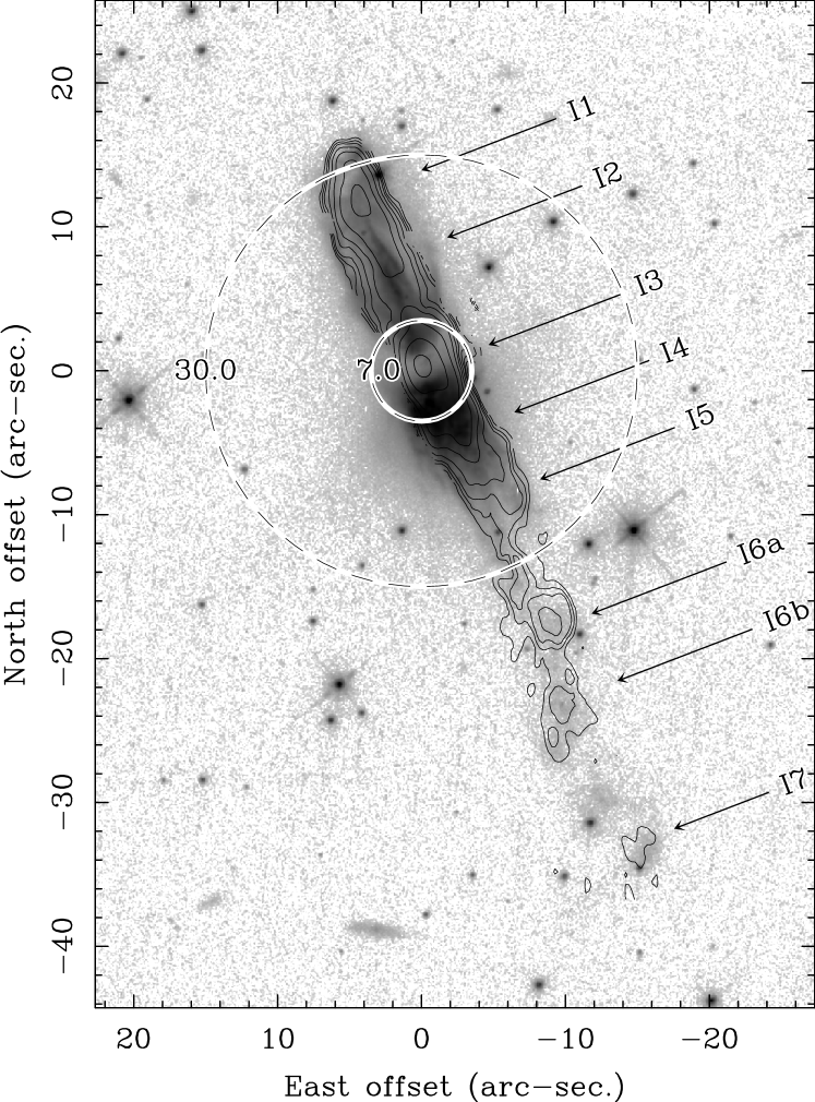
Figure 1: Composite image of OH 231.8$+$4.2 displaying: (grey scale) the dust distribution as observed with $HST$/WFPC2 and the broad-band F791W filter (Bujarrabal et al., 2002); (contours) the molecular outflow as traced by the ¹²CO (2–1) emission (velocity integrated) mapped with 1$\aas@@fstack{\prime\prime}$5$\times$0$\aas@@fstack{\prime\prime}$7-resolution (see Fig. 4 in Alcolea et al., 2001). The dashed circles show the area covered by the largest and smallest telescope beams (HPBW) of the IRAM-30 m observations presented in this work. The different emitting clumps, I1-I7, are labelled as in Alcolea et al. (2001). The $V_{\mathrm{LSR}}$ range (in km s^-1) of each clump is I1) [$-$80:$-$30], I2) [$-$30:$+$10], I3) [$+$10:$+$55], I4) [$+$55:$+$80], I5) [$+$80:$+$150], I6a) [$+$150:$+$205], I6b) [$+$205:$+$230], and I7) [$+$230:$+$285] (see Table 2 in Alcolea et al., 2001, for more details on the physical properies of the clumps).

Most of the nebular material of OH 231.8$+$4.2 is in the form of dust and molecular gas, which are best traced by scattered starlight and by the emission from rotational transitions of CO, respectively (see e.g. Sánchez Contreras et al., 1997; Alcolea et al., 2001; Bujarrabal et al., 2002). The molecular gas is cool ($\sim$10–40 K over the bulk of the nebula) and massive ($\sim$1 $M_{\odot}$). With a spatial distribution similar to that of dust, this gas is located in a very elongated and clumpy structure with two major components (Fig. 1): ($i$) a central core (clump I3) with an angular diameter of $\sim$6-8″, a total mass of $\sim$0.64 $M_{\odot}$, and low expansion velocity ($\sim$6-35 km s^-1), and ($ii$) a highly collimated $\la$6^′′$\times$57^′′ bipolar outflow, with a total mass of $\sim$0.3$M_{\odot}$ and expansion velocities that increase linearly with the distance from the centre, reaching values of up to $\sim$200 and 430 km s^-1 at the tip of the northern and southern lobes, respectively. The temperature in the lobes is notably low, $\sim$10-20 K (Sánchez Contreras et al., 1997; Alcolea et al., 2001). A shock-excited atomic/ionized gas nebulosity, hotter ($\sim$10,000 K) but far less massive ($\sim$2$\times$10^-3 $M_{\odot}$), surrounds the front edges of the molecular outflow delineating two inflated bubble-like, asymmetric lobes (not shown in Fig. 1; see Reipurth, 1987; Sánchez Contreras et al., 2000a; Bujarrabal et al., 2002; Sánchez Contreras et al., 2004).

The molecular envelope of OH 231.8$+$4.2 is remarkably different from the slow, roughly round winds of most AGB stars; however, its pronounced axial symmetry, high expansion velocities, and the presence of shocks are common in objects that have left the AGB phase and are evolving to the PN stage, so-called pre-PNs (Neri et al., 1998; Bujarrabal et al., 2001; Castro-Carrizo et al., 2010; Sánchez Contreras & Sahai, 2012). It is believed that the nebula of OH 231.8$+$4.2 was created as the result of a huge mass loss that occurred during the late-AGB evolution of the primary at a rate of $\dot{M}$$\approx$10^-4 $M_{\odot}$ yr^-1. With a total linear momentum of $\sim$27 $M_{\odot}$km s^-1, the bipolar flow is interpreted as the result of a sudden axial acceleration of the envelope. It is probable that such an acceleration resulted from the violent collision between underlying jets (probably emanating from the stellar companion) on the slowly expanding AGB envelope (Sánchez Contreras et al., 2000b; Alcolea et al., 2001; Bujarrabal et al., 2002; Sánchez Contreras et al., 2004); this is one plausible scenario that has been proposed to explain the shaping and acceleration of bipolar pre-PNs and PNs (e.g. Sahai & Trauger, 1998; Balick & Frank, 2002). Recently, Sabin et al. (2014) have found indications of a well-organized magnetic field parallel to the major axis of the CO-outflow that could point to a magnetic-outflow launching mechanism. As mentioned by these authors, the magnetic field could have, alternatively, been dragged by the fast outflow, which may have been launched by a different mechanism. The linear distance-velocity relation observed in the CO-outflow (with a projected velocity gradient of $\nabla V$$\sim$6.5 km s^-1 arcsec^-1) suggests that the acceleration of the lobes took place $\sim$ 800 yr ago in less than $\sim$150 yr. The low-velocity central core is thought to be the fossil remnant of the AGB CSE.

OH 231.8$+$4.2 is the chemically richest CSE around an O-rich low/intermediate mass evolved star. In addition to the typical oxygen-rich content, with molecules such as H₂O, OH, or SiO (Bowers & Morris, 1984; Morris et al., 1987; Zijlstra et al., 2001; Sánchez Contreras et al., 2002; Desmurs et al., 2007), it displays strong lines of many different molecular species, including many containing carbon. The full inventory of the molecules reported in OH 231.8$+$4.2 prior to our survey are ¹²CO, ¹³CO, SO, SO₂, H₂O, OH, SiO, H₂S, HCN, H¹³CN, HNC, CS, HCO⁺, H¹³CO⁺,OCS, H₂CO, NH₃, and NS (Ukita & Morris, 1983; Guilloteau et al., 1986; Morris et al., 1987; Omont et al., 1993; Sánchez Contreras et al., 1997; Lindqvist et al., 1992; Sánchez Contreras et al., 2000b, and references therein). High-angular resolution mapping of the HCO⁺ ($J$=1–0) emission indicates that this ion is present in abundance in the fast lobes (Sánchez Contreras et al., 2000b). Based on single-dish maps of the SiO ($J$=5–4) emission, the abundance of this molecule could also be enhanced in the lobes (Sánchez Contreras et al., 1997). The spectrum of OH 231.8$+$4.2 is unusually rich, even for O-rich CSEs’ standards, in lines from S- and N-bearing molecules (for example, it was the first O-rich CSE in which H₂S, NS, CS, and OCS were detected.) Some of these S- and N-compounds are present in the envelope at relatively high levels, for example, SO₂ and HNC (see references above). It is believed that extra Si and S are released into the gas phase from dust grains by shocks. Shocks might also initiate (endothermic) reactions that trigger the N and S chemistry and could also be additional suppliers of free atoms and ions (Morris et al., 1987).

2 Observations

The observations presented in this paper are part of a sensitive mm-wavelength ($\sim$79-356 GHz) survey carried out with the IRAM-30 m  telescope (Pico Veleta, Granada, Spain) towards the CSEs of two O-rich evolved stars: OH 231.8$+$4.2  and IK Tau. Preliminary results from this survey are reported in Sánchez Contreras et al. (2011) and Velilla Prieto et al. (2013).

We used the new-generation heterodyne Eight MIxer Receiver (EMIR), which works at four different mm-wavelength bands, E090=3 mm, E150=2 mm, E230=1 mm, and E330=0.9 mm (Carter et al., 2012). EMIR was operated in single-sideband (SSB) mode for band E150 and in dual sideband (2SB) mode for bands E090, E230, and E330. E090 and E150 were observed simultaneously providing 8 GHz and 4 GHz instantaneous bandwidths, respectively. E330 was also observed simultaneously with E150, providing 16 GHz of instantaneous bandwidth, and E230 was observed alone, providing 16 GHz of instantaneous bandwidth.

Each receiver band was connected to different spectrometers; here we report data observed with the WILMA autocorrelator, which provides a spectral resolution of 2 MHz (i.e. 7.5-1.7 km s^-1 in the observed frequency range, 79-356 GHz), and the fast Fourier transform spectrometer (FTS) in its 195 kHz spectral resolution mode (i.e. 0.7-0.2 km s^-1). Both spectrometers provide full coverage of the instantaneously available frequencies.

For each band, the two orthogonal polarizations were observed simultaneously for a series of tuning steps until we covered the total frequency range accessible to each band. The central frequencies of the different tuning steps were chosen to provide a small frequency overlap between adjacent tunings. The average rejection of the image band signal was measured to be $\sim$14 dB, in agreement with the typical values for EMIR; this implies that the peak intensity of a line entering through the image band is only $\sim$4 % of its real value.

Observations were performed towards the centre of the nebula (R.A.2000=$07^{h}42^{m}16^{s}.93$, Dec.2000=$-14^{\circ}42^{{}^{\prime}}50^{{}^{\prime\prime}}.20$). We used the wobbler switching mode, with a wobbler throw of 120″ in azimuth. The beamwidth of the antenna is in the range $\sim$30″-7″at the observed frequencies (Table 1). These observations thus provide spectra that are spatially integrated over the slow central core of OH 231.8$+$4.2 (clump I3, from which the bulk of the molecular emission arises), and more or less depending on the observed frequency, from the fast bipolar outflows, always leaving out the emission from the most distant and, thus, fastest and most tenuous clumps (I6-I7) in the southern lobe (see Fig. 1).

Table 1: Main parameters of the IRAM-30 m EMIR receiver at representative frequencies.

Frequency	Beam eff.	Forward eff.	HPBW	S/T${}_{a}^{*}$
(GHz)	(%)	(%)	(”)	(Jy/K)
86	81	95	29	5.9
145	74	93	17	6.4
210	63	94	12	7.5
340	35	81	7	10.9

Pointing and focus were checked regularly (every $\sim$1.5 and $\sim$4 h, respectively) on strong nearby sources. On-source integration times per tuning step were $\sim$1 h. Additional information on the observations is provided in Table 2.

Table 2: Relevant observational information.

Band	Mode	IBW	$\nu_{obs}$	rms	Opacity
		(GHz)	(GHz)	(mK)
E090	2SB	8	79.3 - 115.7	1 - 3	0.07 - 0.38
E150	SSB	4	128.4 - 174.8	2 - 8	0.03 - 0.39
E230	2SB	16	202.1 - 270.7	5 - 10	0.12 - 0.30
E330	2SB	16	258.4 - 356.2	6 - 24	0.07 - 0.76

Calibration scans on the standard two load + sky system were taken every $\sim$18 min; the atmospheric transmission is modelled at IRAM-30 m using ATM (Cernicharo et al., 1985; Pardo et al., 2001). All spectra have been calibrated on the antenna temperature (T${}^{*}_{\rm A}$) scale, which is related to the mean brightness temperature of the source ($T_{\rm B}$) via the equation

$$T_{\rm B}=T^{*}_{\rm A}\;\frac{F_{\rm eff}}{B_{\rm eff}}\;\delta^{-1}=T_{\rm mb}\;\delta^{-1}$$ (1)

where T_mb is the main-beam temperature, $F_{eff}$ and $B_{eff}$ are the forward efficiency and the main-beam efficiency of the telescope, respectively, and $\delta$ is the beam-filling factor. The ratio between $F_{eff}$ and $B_{eff}$ is described by the equation

$$\frac{F_{\rm eff}}{B_{\rm eff}}=1.1e^{\,(\nu(GHz)/398.5)^{2}}.$$ (2)

The molecular outflow of OH 231.8$+$4.2 has been assumed to be a uniform elliptical source with major and minor axes $\theta_{\rm a}$ and $\theta_{\rm b}$. In this case, the beam-filling factor is given by (see e.g. Kramer, 1997):

$$\delta=1-e^{-\ln 2\frac{\theta_{\rm a}\times\theta_{\rm b}}{HPBW^{2}}}$$ (3)

where $HPBW$ is the half power beam width of an elliptical Gaussian beam. Based on previous maps of CO and other molecules, we adopt an angular source size of $\theta_{\rm a}$$\times$$\theta_{\rm b}$=4″$\times$12″.

We have checked the relative calibration between adjacent frequency tunings by comparing the intensities of the lines in the overlap regions and in frequency tunings that were observed in different epochs. An extra check of the calibration has been made by comparing the intensities of the ¹²CO and ¹³CO lines from this survey with those measured in previous observations (Morris et al., 1987; Sánchez Contreras et al., 1997). Errors in the absolute flux calibration are expected to be $\la$25%.

Data were reduced using CLASS to obtain the final spectra. We followed the standard procedure, which includes flagging of bad channels, flagging of low-quality scans, baseline substracting, averaging individual scans, and channel smoothing to a typical spectral resolution of ($\sim$2 MHz).

Table 3: Parameters of the lines detected in OH 231.8$+$4.2 reported in this work.

Molecule	Transition	$\nu_{\mathrm{rest}}$	$E_{\mathrm{u}}$	$A_{\mathrm{ul}}$	$\int T_{\mathrm{mb}}^{*}\,d\mathrm{v}$	FWHM	Tmb,peak
	quantum numbers	(MHz)	(K)	s-1	(K km s-1)	(km s-1)	(mK)
13CO	1 $\rightarrow$ 0	110201.35	5.3	6.336$\times$10-8	12.81(0.05)	36.1(0.4)	324(2)
$J$	2 $\rightarrow$ 1	220398.68	15.9	6.082$\times$10-7	69.63(0.13)	32.4(0.4)	1818(9)
	3 $\rightarrow$ 2	330587.96	31.7	2.199$\times$10-6	87.6(0.6)	29.5(0.4)	2420(50)
HNCO	40,4 $\rightarrow$ 30,3	87925.24	10.5	9.025$\times$10-6	1.31(0.05)	32.0(1.3)	32.8(1.6)
$J_{K_{\mathrm{a}},K_{\mathrm{c}}}$	50,5 $\rightarrow$ 40,4	109905.75	15.8	1.802$\times$10-5	2.54(0.06)	33.2(0.7)	61.3(1.8)
	60,6 $\rightarrow$ 50,5	131885.73	22.2	3.163$\times$10-5	3.64(0.05)	29.4(0.5)	93.7(2.1)
	70,7 $\rightarrow$ 60,6	153865.09	29.5	5.078$\times$10-5	4.83(0.06)	28.6(0.4)	140(3)
	100,10 $\rightarrow$ 90,9	219798.27	58.0	1.510$\times$10-4	6.67(0.14)	24.5(0.9)	200(9)
	110,11 $\rightarrow$ 100,10	241774.03	69.6	2.019$\times$10-4	7.32(0.14)	21.5(0.5)	260(8)
	120,12 $\rightarrow$ 110,11	263748.62	82.3	2.630$\times$10-4	4.73(0.22)	21.3(1.0)	179(14)
	130,13 $\rightarrow$ 120,12	285721.95	96.0	3.355$\times$10-4	6.3(0.4)
	140,14 $\rightarrow$ 130,13	307693.90	110.8	4.200$\times$10-4	2.48(0.20)	19.9(1.6)	114(16)
	51,5 $\rightarrow$ 41,4	109495.99	59.0	1.692$\times$10-5	0.08(0.04)	13(6)	4.8(2.1)
	61,6 $\rightarrow$ 51,5	131394.23	65.3	3.006$\times$10-5	0.22(0.02)	14(4)	7.6(1.4)
	61,5 $\rightarrow$ 51,4	132356.70	65.5	3.072$\times$10-5	0.16(0.03)	14(9)	5.5(1.8)
	71,7 $\rightarrow$ 61,6	153291.94	72.7	4.863$\times$10-5	0.25(0.04)	9(4)	15.8(2.2)
	71,6 $\rightarrow$ 61,5	154414.76	72.9	4.971$\times$10-5	0.28(0.03)	18(7)	6.5(2.1)
	111,11 $\rightarrow$ 101,10	240875.73	112.6	1.957$\times$10-4	0.35(0.10)	12(2)	34(8)
	121,12 $\rightarrow$ 111,11	262769.48	125.3	2.554$\times$10-4	0.31(0.09)	12(3)	22(11)
	131,13 $\rightarrow$ 121,12	284662.17	138.9	3.261$\times$10-4	0.28(0.07)	14(3)	20(10)
HNCS	80,8 $\rightarrow$ 70,7	93830.07	20.3	1.217$\times$10-5	0.19(0.04)	27(9)	4.4(2.0)
$J_{K_{\mathrm{a}},K_{\mathrm{c}}}$	90,9 $\rightarrow$ 80,8	105558.08	25.3	1.744$\times$10-5	0.23(0.04)		4.0(1.6)
	110,11 $\rightarrow$ 100,10	129013.26	37.2	3.215$\times$10-5	0.32(0.04)	33(5)	8.5(2.2)
	120,12 $\rightarrow$ 110,11	140740.38	43.9	4.189$\times$10-5	0.26(0.04)	34(9)	4.7(2.3)
	130,13 $\rightarrow$ 120,12	152467.14	51.2	5.342$\times$10-5	0.30(0.04)	18(2)	14.8(2.1)
	140,14 $\rightarrow$ 130,13	164193.52	59.1	6.690$\times$10-5	0.34(0.02)	21(1)	15.1(1.4)
HC3N	9 $\rightarrow$ 8	81881.46	19.6	4.215$\times$10-5	0.30(0.06)	27(6)	7.5(2.3)
$J$	10 $\rightarrow$ 9	90978.99	24.0	5.812$\times$10-5	0.38(0.03)	26(5)	8.5(1.5)
	11 $\rightarrow$ 10	100076.38	28.8	7.770$\times$10-5	0.44(0.04)	28(3)	12.4(1.7)
	12 $\rightarrow$ 11	109173.64	34.1	1.012$\times$10-4	0.15(0.03)
	15 $\rightarrow$ 14	136464.40	52.4	1.993$\times$10-4	0.35(0.03)	16(2)	17.8(1.9)
	16 $\rightarrow$ 15	145560.95	59.4	2.424$\times$10-4	0.29(0.04)	17(3)	12(3)
	17 $\rightarrow$ 16	154657.29	66.8	2.912$\times$10-4	0.20(0.04)	20(4)	9.6(2.3)
	18 $\rightarrow$ 17	163753.40	74.7	3.463$\times$10-4	0.25(0.03)	22(5)	10.7(2.1)
NO	$\Pi^{+}$(3/2,5/2) $\rightarrow$ (1/2,3/2)	150176.48	7.2	3.310$\times$10-7 }50.1pt[]	1.15(0.08)	55(10)	9(3)
$\Pi^{\mathrm{band}}(J,F)$	$\Pi^{+}$(3/2,3/2) $\rightarrow$ (1/2,1/2)	150198.76	7.2	1.839$\times$10-7
	$\Pi^{+}$(3/2,3/2) $\rightarrow$ (1/2,3/2)	150218.73	7.2	1.471$\times$10-7
	$\Pi^{+}$(3/2,1/2) $\rightarrow$ (1/2,1/2)	150225.66	7.2	2.943$\times$10-7
	$\Pi^{+}$(3/2,1/2) $\rightarrow$ (1/2,3/2)	150245.64	7.2	3.679$\times$10-8
	$\Pi^{-}$(3/2,3/2) $\rightarrow$ (1/2,1/2)	150644.34	7.2	1.853$\times$10-7	0.20(0.03)	39(9)	4.9(2.1)
	$\Pi^{+}$(5/2,7/2) $\rightarrow$ (3/2,5/2)	250436.85	19.2	1.841$\times$10-6 }50.1pt[]	5.08(0.16)	54(2)	82(9)
	$\Pi^{+}$(5/2,5/2) $\rightarrow$ (3/2,3/2)	250440.66	19.2	1.547$\times$10-6
	$\Pi^{+}$(5/2,3/2) $\rightarrow$ (3/2,1/2)	250448.53	19.2	1.381$\times$10-6
	$\Pi^{+}$(5/2,3/2) $\rightarrow$ (3/2,3/2)	250475.41	19.2	4.420$\times$10-7
	$\Pi^{+}$(5/2,5/2) $\rightarrow$ (3/2,5/2)	250482.94	19.2	2.947$\times$10-7
	$\Pi^{-}$(5/2,7/2) $\rightarrow$ (3/2,5/2)	250796.44	19.3	1.849$\times$10-6 }30.1pt[]	4.77(0.15)	64(2)	68(9)
	$\Pi^{-}$(5/2,5/2) $\rightarrow$ (3/2,3/2)	250815.59	19.3	1.554$\times$10-6
	$\Pi^{-}$(5/2,3/2) $\rightarrow$ (3/2,1/2)	250816.95	19.3	1.387$\times$10-6
	$\Pi^{+}$(7/2,9/2) $\rightarrow$ (5/2,7/2)	350689.49	36.1	5.418$\times$10-6 }50.1pt[]	7.2(0.5)	40(4)	149(40)
	$\Pi^{+}$(7/2,7/2) $\rightarrow$ (5/2,5/2)	350690.77	36.1	4.976$\times$10-6
	$\Pi^{+}$(7/2,5/2) $\rightarrow$ (5/2,3/2)	350694.77	36.1	4.815$\times$10-6
	$\Pi^{+}$(7/2,5/2) $\rightarrow$ (5/2,5/2)	350729.58	36.1	5.897$\times$10-7
	$\Pi^{+}$(7/2,7/2) $\rightarrow$ (5/2,7/2)	350736.78	36.1	4.423$\times$10-7
	$\Pi^{-}$(7/2,9/2) $\rightarrow$ (5/2,7/2)	351043.52	36.1	5.433$\times$10-6 }30.1pt[]	5.2(0.5)	41(5)	122(40)
	$\Pi^{-}$(7/2,7/2) $\rightarrow$ (5/2,5/2)	351051.47	36.1	4.990$\times$10-6
	$\Pi^{-}$(7/2,5/2) $\rightarrow$ (5/2,3/2)	351051.70	36.1	4.830$\times$10-6

3 Observational results

Line identification over the full frequency range covered in this survey was done using the public line catalogues from the Cologne Database for Molecular Spectroscopy (CDMS, Müller et al., 2005) and the Jet Propulsion Laboratory (JPL, Pickett et al., 1998), together with a private spectroscopic catalogue that assembles information for almost five thousand spectral entries (molecules and atoms), including isotopologues and vibrationally excited states, compiled from extensive laboratory and theoretical works by independent teams (Cernicharo, 2012).

We have identified hundreds of transitions from more than 50 different molecular species including their main isotopologues (¹³C-, ¹⁸O-, ¹⁷O-, ³³S-, ³⁴S-, ³⁰Si, and ²⁹Si) in OH 231.8$+$4.2, confirming the chemical richness of this source, which is unprecedented amongst O-rich AGB and post-AGB stars.

First detections from this survey include the N-bearing species HNCO, HNCS, HC₃N, and NO, which are the focus of this paper. Together with these, we present the spectra of the ¹³CO $J$=1–0, $J$=2–1, and $J$=3–2 transitions, which are excellent tracers of the mass distribution and dynamics in OH 231.8$+$4.2: ¹³CO lines are optically thin (or, at most, moderately opaque towards the nebula centre) and are expected to be thermalised over the bulk of the outflow and, certainly, in the regions that lie within the telescope beam in these observations, characterized by average densities always above 10⁴ cm^-3 (Sánchez Contreras et al., 1997; Alcolea et al., 2001). Spectra of different rotational transitions from the ground vibrational state ($v=0$) of ¹³CO, HNCO, HNCS, HC₃N, and NO are shown in Figs. 2-7, and main line parameters are reported in Table 3.

Figure 2: ¹³CO mm-wavelength transitions in OH 231.8$+$4.2. We labelled the different spectral features in the ¹³CO profiles as I1-I5 to identify them with the corresponding regions/clumps of CO-outflow where the emission features mainly arise (see Fig. 1). In the top panel, the ¹³CO $J$=1–0 spectrum is also plotted using a larger T_mb scale for an improved view of the weak broad wings.

3.1 ¹³CO spectra

The ¹³CO lines (Fig. 2) show broad, structured profiles with two main components: (1) the intense, relatively narrow (FWHM$\sim$30-35 km s^-1) core centred at $V_{\mathrm{LSR}}$=33.4$\pm$0.9km s^-1, which arises in the slow, dense central parts of the nebula (clump I3); and (2) weak broad wings, with full widths of up to $\sim$220 km s^-1 in the $J$=1–0 line, which originate in the fast bipolar lobes clumps I1-I2 and I4-I5). The most intense spectral component in the ¹³CO wings arises at clump I4, i.e. the base of the southern lobe, and the I4/I3 feature peak-intensity ratio is I4/I3$\sim$0.3. The single-dish profiles of the $J$=1–0 and 2–1 lines are already known from previous observations (Morris et al., 1987; Sánchez Contreras et al., 1997) and, within the expected calibration errors, are consistent with those observed in this survey.

The full width of the wings is largest for the ¹³CO ($J$=1$-$0) transition, which is observed over a velocity range of $V_{\mathrm{LSR}}$=[$-$80:$+$140] km s^-1, and decreases for higher-$J$ transitions down to $V_{\mathrm{LSR}}$=[$-$10:$+$90] km s^-1  for the $J$=3–2 line. The different width of the wings is partially explained by the increase in the expansion velocity with the distance to the centre along the CO outflow and the smaller beam for higher frequencies. Also, as can be observed (Fig. 2 and Table 3), the FWHM of the ¹³CO  transitions decrease as the upper energy level increases. This suggests that the envelope layers with higher excitation conditions (i.e. warmer and, thus, presumably closer to the central star) are characterized by lower expansion velocities. This trend is confirmed by higher frequency transitions of ¹³CO (and of most molecules) observed with Herschel with a larger telescope beam (e.g. Bujarrabal et al., 2012; Sánchez Contreras et al., 2014).

3.2 New N-bearing molecules

Isocyanic acid (HNCO) is a quasi-linear asymmetric rotor whose structure was first determined by Jones et al. (1950). It contains a nitrogen atom that has a nuclear spin ($I$=1) leading to a splitting of each rotational level. This hyperfine (hpf) structure is not resolved since the maximum separation in velocity of the hpf components from the most intense one is $\la$2 km s^-1, that is, much less than the expansion velocity of the envelope (and, in some cases, even smaller than the spectral resolution of our observations). The rotational levels of HNCO are expressed in terms of three quantum numbers: $J$ the rotational quantum number, $K_{\mathrm{a}}$ and $K_{\mathrm{c}}$, which are the projections of $J$ onto the A and C molecular axes, respectively. We have detected several a-type transitions (i.e. with $\Delta K_{\mathrm{a}}$=0 and $\Delta K_{\mathrm{c}}$=$\pm$1) in the $K_{\mathrm{a}}$=0 and $K_{\mathrm{a}}$=1 ladders (Figs. 3,4); the difference between the $K_{\mathrm{a}}$=0 zero level and the $1_{1,1}$ level is $\Delta E$=44.33 K. The profiles of the HNCO transitions detected of the $K_{\mathrm{a}}$=0 and $K_{\mathrm{a}}$=1 ladders show notable differences: the $K_{\mathrm{a}}$=0 transitions, which are stronger than the $K_{\mathrm{a}}$=1 ones, show an intense central core component centred at $V_{\mathrm{LSR}}$=29.5$\pm$1.5 km s^-1 and with a line width of FWHM$\sim$20-33 km s^-1; as for ¹³CO, the linewidth decreases as the transition upper level energy increases. In addition to the line core (arising in the central parts of the nebula, clump I3), the HNCO $K_{\mathrm{a}}$=0 profiles show red-wing emission from the base of the southern lobe, clump I4; the I4/I3 feature peak-intensity ratio is $\sim$0.3. The HNCO $K_{\mathrm{a}}$=1 transitions, centred on $V_{\mathrm{LSR}}$=29.5$\pm$1.1km s^-1, are not only weaker but narrower (FWHM$\sim$13 km s^-1) than the $K_{\mathrm{a}}$=0 lines.

Figure 3: HNCO transitions of the $K_{\mathrm{a}}$=0 ladder detected in OH 231.8$+$4.2. Spectral features have been labelled as in Fig. 2. The HNCO $13_{0,13}-12_{0,12}$ transition is blended with the SO₂ $17_{3,15}-17_{2,16}$ line (central, bottom panel).

Figure 4: Same as in Fig. 3 but for the $K_{\mathrm{a}}=1$ ladder. The S/N of some of these transitions is low, so they may be considered as tentative detections; however, in spite of the large errobars, the intensity, centroid $V_{\mathrm{LSR}}$, and FWHM of the tentative lines are consistent with the trend and values deduced for transitions detected with higher S/N.

Isothiocyanic acid (HNCS) presents a structure similar to HNCO; i.e.,  it is a slightly asymmetric rotor (Jones & Badger, 1950). Its hpf structure due to the nitrogen nuclear spin is not spectrally resolved in our data. We have detected several a-type (i.e. with $\Delta K_{\mathrm{a}}$=0 and $\Delta K_{\mathrm{c}}$=$\pm$1) transitions of the $K_{\mathrm{a}}$=0 ladder (Fig. 5). These lines are weak and narrow, with a median FWHM$\sim$25 km s^-1, and are centred at $V_{\mathrm{LSR}}$=28.2$\pm$0.4 km s^-1, indicating that the emission observed arises mainly in the slow central parts of the nebula. HNCS wing emission from the fast flow (if present) is below the noise level. We have not detected any of the $K_{\mathrm{a}}$=1 transitions of HNCS in the frequency range covered by us. These transitions have upper-level state energies $E_{\mathrm{u}}$$\ga$78 K and expected intensities well below our detection limit.

Cyanoacetylene (HC₃N) is a linear molecule that belongs to the nitriles family. We do not resolve its hpf structure spectrally (which is due to the nitrogen nuclear spin), so its rotational levels are described only by the rotational number $J$ (Westenberg & Wilson, 1950). The spectra of the HC₃N transitions detected in OH 231.8$+$4.2 are shown in Fig. 6. The line profiles are centred at $V_{\mathrm{LSR}}$=28.0$\pm$0.9 km s^-1 and are relatively narrow, with typical line widths of FWHM$\sim$22 km s^-1. Tentative emission from clump I4 (at $V_{\mathrm{LSR}}$$\sim$60-65 km s^-1) is observed in most profiles, with a I4/I3 feature peak-intensity ratio of $\sim$0.2-0.4.

Nitric oxide (NO) is a radical with a ${}^{2}\Pi$ ground state that splits into two different ladders, $\Omega$=1/2 (${}^{2}\Pi_{1/2}$) and $\Omega$=3/2 (${}^{2}\Pi_{3/2}$), owing to the unpaired electron by spin-orbit coupling. Additionally, $\Lambda$-doubling means that each transition is split into two different bands of opposite parity $\Pi^{+}$ and $\Pi^{-}$. NO also presents hpf structure owing to the nitrogen nuclear spin that interacts with the total angular momentum, thereby splitting each single rotational level into $2(I,J)_{\rm min}$+1 levels described by the quantum number $F$ (for a complete description of the structure and spectroscopy of the NO rotational transitions see Lique et al., 2009, and references therein). We have detected several transitions of the ${}^{2}\Pi_{1/2}$ ladder around 150, 250, and 350 GHz (see Fig. 7). Transitions of the ${}^{2}\Pi_{3/2}$ ladder, with upper level state energies above 180 K, are not detected. As shown in Fig. 7, each of the $\Lambda$-doublets ($\Pi^{+}$ and $\Pi^{-}$) of NO is composed of several hpf components that are blended in our spectra, except for the $\Pi^{-}$ $(3/2,3/2)-(1/2,1/2)$ line at 150.644 GHz, which is isolated.

The NO blends appear on average redshifted by a few km s^-1 from the source systemic velocity and are broader than the profiles of the other N-bearing species discussed in this work. The broadening is partially (but not only) due to the hpf structure of the NO transitions. To constrain the intrinsic linewidth and centroid of the individual hpf components contributing to the observed profile, we have calculated and added together the emergent spectrum of the hpf components. The synthetic spectrum was calculated using our code MADEX (Cernicharo, 2012, see also Appendix A) and also the task MODSOURCE of CLASS, both giving similar results at LTE (non-LTE calculations are available in MADEX but not in MODSOURCE). We adopted a Gaussian profile for the hpf lines.

Figure 5: Same as in Fig. 3 but for HNCS.

We find that, first, the shape of the NO blends cannot be reproduced by adopting sharply centrally peaked profiles such as those of HNCO, HNCS, and HC₃N, with line centroids at $V_{\mathrm{LSR}}$$\sim$28-29 km s^-1 and widths of FWHM$\sim$15-30 km s^-1 (dotted line in Fig. 7). In order to match the profiles of the NO blends, the individual hpf components must have a larger width of FWHM$\sim$40-50 km s^-1 and must be centered at $V_{\mathrm{LSR}}$$\sim$35-40 km s^-1 (Fig. 7). In support of this conclusion, a Gaussian fit to the $\Pi^{-}$ $(3/2,3/2)-(1/2,1/2)$ line at 150.644 GHz, which is unblended, also indicates a broad profile, with a FWHM=40$\pm$8 km s^-1, centred at $V_{\mathrm{LSR}}$=41$\pm$4 km s^-1. Although the intrinsic linewidth is uncertain, the broad profiles of NO indicate that this molecule is present in abundance in the high-velocity lobes and that the wing-to-core emission contribution is greater for NO than for HNCO, HNCS, and HC₃N. In particular, an important part of the NO emission profile arises at clump I4. The emission from feature I4 is indeed comparable to that of the narrow core (I3), with an estimated I4/I3 feature peak-intensity ratio of $\sim$1 at 150 GHz, $\sim$0.6-0.8 at 250 GHz, and $\sim$0.5-0.6 at 350 GHz. This significant NO emission contribution from clump I4 to the total profile is one explanation for the apparent overall redshift of the NO lines to an intermediate velocity between that of I3 and I4.

Figure 6: Same as in Fig. 3 but for HC₃N. The poor baseline in the spectrum of the $J$=12–11 line makes the detection of this transition tentative.

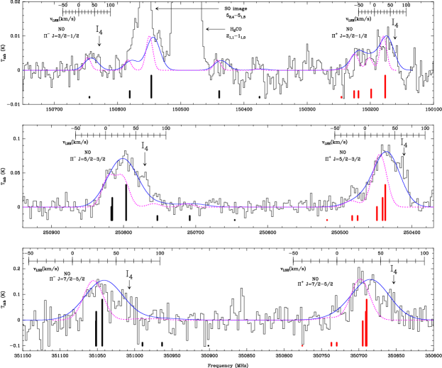
Figure 7: Spectra of the NO transitions detected in OH 231.8$+$4.2. The quantum numbers indicated in this plot for NO are $\Pi$ and $J$ (Table 3). Vertical thick segments indicate the rest frequency and relative strength of the individual hyperfine (hpf) components within each $\Pi^{+}$ and $\Pi^{-}$ blend (red and black, respectively). The LSR velocity scale is shown on top of the NO transitions that have been detected (the velocity scale refers to the strongest hpf component in each case). The LSR velocity of the emission feature associated to clump I4, at the base of the southern lobe, is indicated. The dotted line is the model spectrum (§ 3.2 and Table 4) assuming that the individual hpf components are centred at $V_{\mathrm{LSR}}$=28 km s^-1, and have an intrinsic width of FWHM=25 km s^-1, similar to the dominant narrow component of the HNCO, HNCS, and HC₃N profiles (Figs. 3-6). These line parameters cannot explain the broad profiles and the apparent overall redshift of the NO blends, which are reproduced better by adopting larger FWHM and $V_{\mathrm{LSR}}$ (solid blue line: representative model with FWHM=50 km s^-1 and $V_{\mathrm{LSR}}$=40 km s^-1).

4 Data analysis: molecular abundances

In the following sections, beam-averaged column densities ($N_{\mathrm{tot}}$) and rotational temperatures ($T_{\mathrm{rot}}$) are obtained from the population diagram method (§ 4.1) and from non-LTE excitation calculations (§ 4.2). We derive fractional abundances ($X$) relative to molecular hydrogen (H₂) for the different molecular species detected in OH 231.8$+$4.2. As a reference, we have used the fractional abundance of ¹³CO, for which we adopt $X$(¹³CO)=5$\times$10^-5 as calculated by Morris et al. (1987). The ¹³CO abundance adopted is in the high end of the typical range of values for O-rich stars; in the case of OH 231.8$+$4.2, it reflects the particularly low ¹²C/¹³C isotopic ratio, $\sim$5-10, measured in this object (and other O-rich CSEs; Sánchez Contreras et al., 2000b; Teyssier et al., 2006; Milam et al., 2009; Ramstedt & Olofsson, 2014, and references therein).

The fractional abundances of the N-bearing species reported in this work have been calculated as

$$\frac{X(m)}{X(^{13}CO)}\,=\,\frac{\mbox{$N_{\mathrm{tot}}$}(m)}{\mbox{$N_{\mathrm{tot}}$}(^{13}CO)},$$ (4)

where $m$ represents the name of the analysed molecule.

4.1 Population diagram analysis

Population (or rotation) diagrams are used to obtain first-order, beam-averaged column densities ($N_{\mathrm{tot}}$) and rotational temperatures ($T_{\mathrm{rot}}$) from the integrated intensities of multiple rotational transitions of a given molecule in the same vibrational state. This method, which is described in detail and extensively discussed by Goldsmith & Langer (1999), among others, relies on two main assumptions: $i$) lines are optically thin, and $ii$) all levels involved in the transitions used are under local thermodynamical equilibrium (LTE) conditions. This assumption implies that the level populations are described by the Boltzmann distribution with a single rotational temperature, $T_{\mathrm{rot}}$, which is equal to the kinetic temperature of the gas ($T_{\mathrm{kin}}$=$T_{\mathrm{rot}}$). Under these assumptions, the line integrated intensity or line flux ($W$) is related to $N_{\mathrm{tot}}$ and $T_{\mathrm{rot}}$ by the following expression:

$$\ln\,\left(\frac{N_{u}}{g_{u}}\right)=\ln\,\left(\frac{3k_{B}W}{8\pi^{3}\,\nu\,S_{ul}\,\mu^{2}}\right)=\ln\,\left(\frac{N}{Z}\right)-\frac{E_{u}}{k_{B}T_{rot}}$$ (5)

where $N_{\mathrm{u}}$ is the column density of the upper level, $g_{\mathrm{u}}$ the degeneracy of the upper level, $W$ the velocity-integrated intensity of the transition, $k_{\mathrm{B}}$ the Boltzmann constant, $\nu$ the rest frequency of the line, $S_{\mathrm{ul}}$ the line strength of the transition, $\mu$ the dipole moment of the corresponding transition, $Z$ the partition function, and $E_{\mathrm{u}}$ is the upper level energy of the transition.

The partition function, Z_rot has been computed for each molecule by explicit summation of

$$Z_{\rm rot}=\displaystyle\sum_{i=0}^{\infty}g_{i}e^{\frac{-E_{i}}{kT}},$$ (6)

for enough levels to obtain accurate values, using the code MADEX (Appendix A). At low temperatures ($\lesssim$50 K), this ensures moderate uncertainties in the column density ($<$5%) as derived from the low-$E_{\mathrm{u}}$ transitions detected, since the contribution of high-energy levels to the partition function is negligible.

The line flux ($W$) has been obtained by integrating the area below the emission profile, typically within the range $V_{\mathrm{LSR}}$$\sim$[0-100] km s^-1, and is given in a source brightness temperature scale ($W$=$\int$T_bdv), obtained from T${}^{*}_{a}$ via Eq. 1. In the case of ¹³CO, $W$ does not include the weak emission from the wings beyond $V_{\mathrm{LSR}}$$\pm$70 km s^-1 since this high-velocity component is not detected in the other molecules. The values for $W$ used to build the population diagrams are given in Table 3.

The beam-filling factor ($\delta$; see Eq. 3) has been computed by adopting a characteristic size for the emitting region of $\Omega_{\mathrm{s}}$=4″$\times$12″ for all molecules. This size is comparable to but slightly less than the angular size (at half intensity) of the CO-outflow measured by Alcolea et al. (2001) – see Fig. 1. In any case, we have checked that the parameters derived from the population diagram do not vary significantly for a range of reasonable values of $\theta_{\rm a}$$\times$$\theta_{\rm b}$$\sim$(3-6)″$\times$(10-18)″.

Figure 8: Population diagram for ¹³CO and best linear fit (dashed line) to the data (filled symbols). Triangles and squares represent data points with and without the opacity correction $C_{\tau}$ applied, respectively (§ 4.1). The values of $T_{\mathrm{rot}}$ and $N_{\mathrm{tot}}$ derived from the fits are indicated in the bottom left corner of the box for the optically thin (lower) and optical depth corrected (upper) approximations. The error bars of the data points include flux uncertainties due to the rms of the spectra and absolute flux calibration, up to $\sim$25% (§ 2).

The population diagrams for the molecules reported in this work and the derived results are shown in Figures 8-9 and Table 4. For ¹³CO we obtain $T_{\mathrm{rot}}$$\sim$13 K and $N_{\mathrm{tot}}$(¹³CO)$\sim$2$\times$10¹⁷ cm^-2. For these values of $T_{\mathrm{rot}}$ and $N_{\mathrm{tot}}$, we expect moderate optical depths at the line centre ($\tau_{\mathrm{110\,GHz}}$$\sim$0.5, $\tau_{\mathrm{220\,GHz}}$$\sim$1.1, and $\tau_{\mathrm{330\,GHz}}$$\sim$0.9, for a typical linewidth of FWHM$\sim$35 km s^-1), which would lead to underestimating both $T_{\mathrm{rot}}$ and $N_{\mathrm{tot}}$. According to this, an opacity correction factor $C_{\tau}$=$\ln$($\tau$/(1-e^-τ)), as defined by, for instance, Goldsmith & Langer (1999), has been introduced in the population diagram, and a new best fit was obtained. This process (of fitting opacity corrected data points and re-computing $C_{\tau}$) was performed iteratively until convergence was reached. The opacity-corrected values derived are $T_{\mathrm{rot}}$$\sim$16 K and $N_{\mathrm{tot}}$(¹³CO)$\sim$3$\times$10¹⁷ cm^-2.

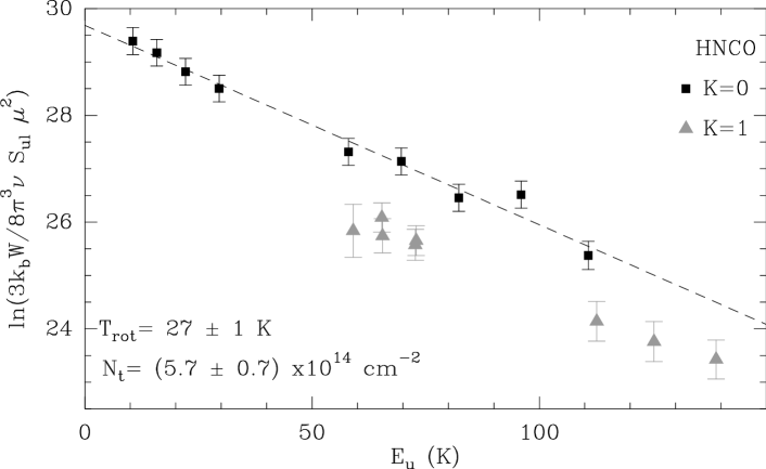
Figure 9: Population diagrams of HNCO, HNCS, HC₃N, and NO (from top to bottom) and best linear fit (dashed line) to the data points (filled symbols; from Table 3). In the case of HNCO, black squares represent transitions with $K_{\mathrm{a}}$=0 and grey triangles the $K_{\mathrm{a}}$=1 transitions. The values of $T_{\mathrm{rot}}$ and $N_{\mathrm{tot}}$ derived from the fit are indicated in the bottom left corner of each box. An opacity correction is not applied in these cases because all the transitions are optically thin. Error bars as in Fig. 8.

In the rotational diagram of HNCO (top panel in Fig. 9), we can clearly see that the transitions of the $K_{a}$=0 and $K_{a}$=1 ladders follow two different trends. Both trends have similar slopes; that is, the $K_{\mathrm{a}}$=0 and $K_{\mathrm{a}}$=1 data points are arranged in two almost parallel straight lines representing similar rotational temperatures. As we show in § 4.2 and Appendix A, the $y$-offset between both lines can be explained by non-LTE excitation effects, which are most prominent in the $K_{\mathrm{a}}$=1 transitions. Using only the HNCO transitions of the $K_{\mathrm{a}}$=0 ladder, we derive $T_{\mathrm{rot}}$$\sim$27 K and $N_{\mathrm{tot}}$(HNCO)$\sim$6$\times$10¹⁴ cm^-2. Following the Eq. (4) and using the ¹³CO opacity corrected column density, we derive a fractional abundance of $X$(HNCO) $\sim$ 1$\times$10^-7.

The rotational diagrams of HNCS, HC₃N, and NO (Fig. 9) show a linear trend, which is consistent with a unique temperature component of $T_{\mathrm{rot}}$$\sim$15-25 K, in agreement with the relatively low value obtained from ¹³CO. There is also good agreement with estimates of $T_{\mathrm{rot}}$ from other molecules such as SO₂ and NH₃ from earlier works (Guilloteau et al., 1986; Morris et al., 1987; Sánchez Contreras et al., 1997). The column densities and fractional abundances derived range between $N_{\mathrm{tot}}$=3$\times$10¹³ cm^-2 and 9$\times$10¹⁵ and $X$=7$\times$10^-9 and 2$\times$10^-6, respectively (see Table 4).

Given the relatively low column densities obtained for HNCO, HNCS, HC₃N, and NO, all the transitions detected are optically thin, so no opacity correction is needed. We note that the high abundance of NO inferred from our data ($\approx$10^-6) is comparable to that of SO₂ and SO, standing amongst the most abundant molecules detected to date in this object (see e.g.  Morris et al., 1987; Sánchez Contreras et al., 2000b, 2014). The second-most abundant molecule reported in this work is HNCO, which is a factor $\sim$20 less abundant than NO and comparable in abundance to HCN and HNC (Morris et al., 1987; Sánchez Contreras et al., 1997, 2000b). The abundance of HNCO is a factor $\sim$10 larger than that of its sulfur analogue, HNCS.

Table 4: Column densities ($N_{\mathrm{tot}}$), rotational temperatures ($T_{\mathrm{rot}}$), and fractional abundances relative to H₂ ($X$) for the molecules detected in OH 231.8$+$4.2 as derived using the population diagram method (§ 4.1) and from non-LTE excitation analysis (§ 4.2). The characteristic angular size for the emitting region adopted is $\Omega_{\mathrm{s}}$=4″$\times$12″.

Molecule	$N_{\mathrm{tot}}$	Trot	$X$
	(cm-2)	(K)
	($i$) LTE RESULTS
13CO	2.6(0.3)$\times$1017	16(1)	5$\times$10-5
HNCO	5.7(0.7)$\times$1014	27(1)	1$\times$10-7
HNCS	7.2(1.2)$\times$1013	23(2)	1$\times$10-8
HC3N	3.5(0.5)$\times$1013	17(1)	7$\times$10-9
NO	8.8(0.7)$\times$1015	22(2)	2$\times$10-6
	($ii$) NON-LTE RESULTS
HNCO	[4.0-5.2]$\times$1014	[26-28]	[0.8-1]$\times$10-7
HNCS	[4.9-7.4]$\times$1013	[23-28]	[0.9-1]$\times$10-8
HC3N	[2.4-3.3]$\times$1013	[45-55]	[5-6]$\times$10-9
NO	[7.5-8.9]$\times$1015	[28-33]	[1-2]$\times$10-6

4.2 Non-LTE excitation

When the local density of molecular hydrogen ($n_{\mathrm{H_{2}}}$) is insufficient to thermalize the transitions of a given molecule, departures from a linear relation in the population diagram are expected. For example, different values of $T_{\mathrm{rot}}$ may be deduced from different transitions, leading to a curvature (or multiple slopes) in the distribution of the data points in the population diagram, which also affects the total column density inferred. Non-LTE excitation effects on the population diagrams of the N-bearing molecules detected in OH 231.8$+$4.2 are investigated and discussed in Appendix A. The high nebular densities in the dominant emitting regions of the outflow ($\sim$10⁵-10⁶  cm^-3) indicate that the ¹³CO lines are thermalized over the bulk of the outflow; however, the transitions observed from HNCO, HNCS, HC₃N, and NO, have critical densities of up to $\sim$10⁶ cm^-3 and, therefore, some LTE deviations may occur. In these cases, the level propulations of the different species are numerically computed (for given input values of $T_{\mathrm{kin}}$, $N_{\mathrm{tot}}$, and $n_{\mathrm{H_{2}}}$) considering both collisional and radiative proceses and the well known LVG approximation – see Appendix A.

In this section, we investigate whether the observations could also be reproduced by values of $T_{\mathrm{kin}}$ and $N_{\mathrm{tot}}$ that are different from those deduced from LTE calculations using moderate $n_{\mathrm{H_{2}}}$ for which LTE does not apply. The results from our non-LTE excitation models have been represented in a population diagram (i.e. N_u/g_u vs. $E_{\mathrm{u}}$) together with the observed data-points. The best data-model fits are shown in Fig. 10, and the range of input values for $T_{\mathrm{kin}}$ and $N_{\mathrm{tot}}$ consistent with the observations are given in Table 4.

Except for HNCO (see below), in our non-LTE models we have adopted a mean characteristic density in the emitting regions of the outflow of $n_{\mathrm{H_{2}}}$$\sim$10⁵ cm^-3. The lowest densities in OH 231.8$+$4.2, $n_{\mathrm{H_{2}}}$$\sim$10³-10⁴ cm^-3, are only found at large distances from the star in the southern lobe (clumps I5 and beyond) that do not contribute to the emission observed from these N-bearing species (Alcolea et al., 2001).

In the case of HNCO, one notable effect of non-LTE conditions is the split of the $K_{\mathrm{a}}$=0 and $K_{\mathrm{a}}$=1 ladders into two almost paralell straight lines in the population diagram (Appendix A). The separation between the $K_{\mathrm{a}}$=0 and $K_{\mathrm{a}}$=1 ladders, which is indeed observed in OH 231.8$+$4.2 (e.g. Fig. 10, top panel), progressively reduces as the density increases; when densities $\ga$10⁸ cm^-3 are reached, all transitions reported here are very close to thermalization, and both the $K_{\mathrm{a}}$=0 and $K_{\mathrm{a}}$=1 ladders merge into one single straight line. The non-LTE excitation analysis of HNCO indicates that the observed separation between the $K_{\mathrm{a}}$=0 and $K_{\mathrm{a}}$=1 ladders in the population diagram of OH 231.8$+$4.2 requires nebular densities of $n_{\mathrm{H_{2}}}$$\sim$4$\times$10⁷ cm^-3. This suggests that most of the observed HNCO emission probably arises at relatively dense regions in the envelope. Adopting $n_{\mathrm{H_{2}}}$$\sim$4$\times$10⁷ cm^-3, therefore, we find that the observations are reproduced well for a range of values of $N_{\mathrm{tot}}$(HNCO)$\sim$[4.0-5.2]$\times$10¹⁴ cm^-2 and $T_{\mathrm{kin}}$$\sim$26-28 K, that is, very similar to those obtained under the LTE approximation.

Several authors have pointed out the importance of infrared pumping to explain the excitation of HNCO under certain conditions (e.g. Churchwell et al., 1986; Li et al., 2013). We have not taken the effect of IR pumping into account given the complexity of the problem, which is beyond the scope of this paper. This effect adds additional uncertainties to the HNCO abundance, which could be larger or smaller than the value quoted in Table 4, but probably by a factor not greater than $\sim$2-5. Additional discussion about this topic is given in the Appendix A.

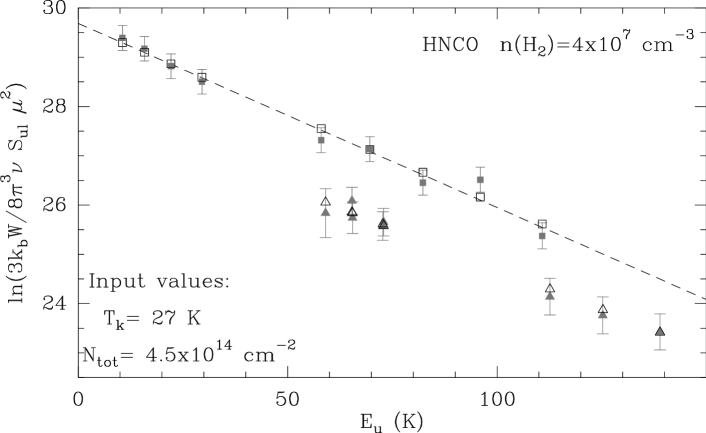
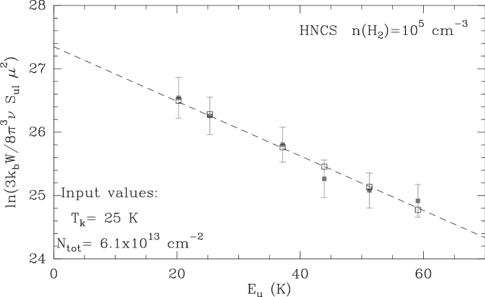
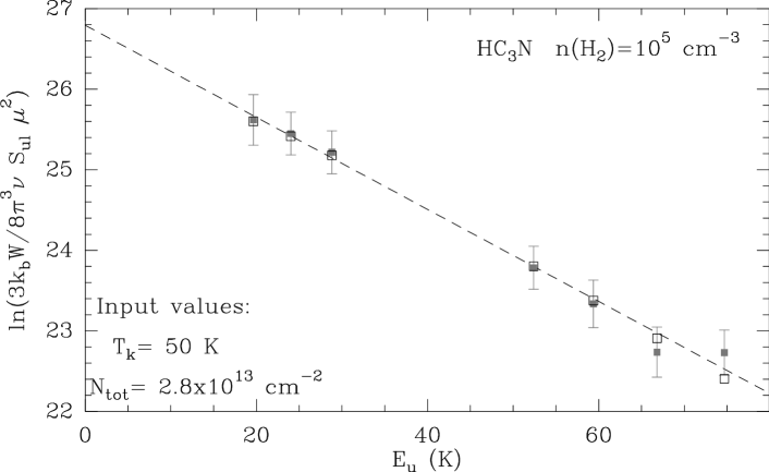
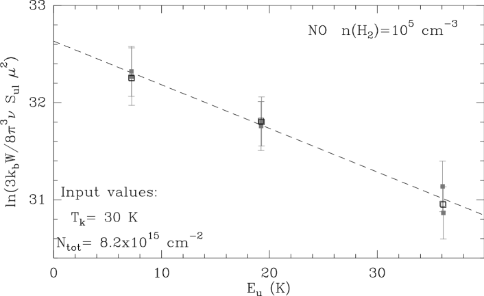
Figure 10: Population diagrams of HNCO, HNCS, HC₃N, and NO including observational data points (filled symbols) and points from representative non-LTE models (empty symbols; § 4.2). The main input parameters ($n_{\mathrm{H_{2}}}$, $T_{\mathrm{kin}}$, and $N_{\mathrm{tot}}$) of the non-LTE models are indicated within the boxes, along with the linear fit to the data points (dashed line; same as in Fig. 9). For HNCO, squares and triangles represent the $K_{\mathrm{a}}$=0 and $K_{\mathrm{a}}$=1 transitions, respectively (as in Fig. 9).

For HNCO and the rest of the molecules, HNCS, HC₃N, and NO, one major effect of non-LTE excitation on the population diagram is a modification of the slope of the straight line defined by the data points (N_u/g_u vs. $E_{\mathrm{u}}$) with respect to the correct value entered as input in the model as $T_{\mathrm{kin}}$. In particular, as can be seen in Fig. 10, for $n_{\mathrm{H_{2}}}$$\sim$10⁵  cm^-3, the rotational temperature that one would deduce from the population diagram is lower than the input kinetic temperature ($T_{\mathrm{rot}}$$<$$T_{\mathrm{kin}}$, sub-thermal excitation). The largest difference between $T_{\mathrm{kin}}$ and $T_{\mathrm{rot}}$ in our models is found for HC₃N; in this case, values of $T_{\mathrm{kin}}$ of up to $\sim$55 K in the emitting regions cannot be ruled out. On the other hand, in general for all species, the column densities derived from the non-LTE excitation analysis are systematically lower than those deduced assuming LTE conditions. We note, however, that these differences are typically $\la$30%.

Finally, as shown in the Appendix A, for densities of $n_{\mathrm{H_{2}}}$$\leq$10⁴  cm^-3, non-LTE level populations of HNCO, HNCS, HC₃N, and NO would result in a double slope in their population diagrams. (This effect would be most prominent for HC₃N.) That this is not observed in our data, described well by a unique value of $T_{\mathrm{rot}}$, corroborates that the typical densities in the emitting regions are above 10⁴  cm^-3.

5 Chemical modelling

In this section, we present thermodynamical chemical equilibrium (TE) and chemical kinetics models to investigate the formation of HNCO, HNCS, HC₃N, and NO in O-rich CSEs with characteristics similar to those in OH 231.8$+$4.2. The TE calculations should provide a good estimation of the molecular abundances near the stellar photosphere, up to $\sim$4-5 $R_{*}$, given the high densities ($\approx$10¹⁴-10⁹  cm^-3) and high temperatures ($\sim$2000 K) expected in these innermost regions (e.g. Tsuji, 1973). As the gas or dust in the stellar wind expands, the temperature and the density gradually decrease, and the chemical timescale increases, making chemical kinetics dominate in determining the molecular abundances. Eventually, the dispersion of the envelope allows the interstellar UV photons to penetrate through the outermost layers, leading to the onset of a productive photo-induced chemistry.

For many important molecules, the abundances established by the equilibrium chemistry in the dense, hot photosphere are expected to be greatly modified by various processes (not all understood well) that operate in the deep envelope layers. First, the inner wind regions at a few $R_{\star}$ are dominated by non-equilibrium reactions triggered by low-velocity shocks generated by the stellar pulsation. Second, the formation of dust particles, which begins farther out at $\sim$5-15$R_{\star}$, well affects the chemistry a lot in different ways, for example, depleting refractory species from the gas phase (owing to grain adsorption) and powering the production of other compounds through grain surface reactions. Because of all this, the molecules produced by these processes in the deep envelope layers, named ‘parent’, are injected to the intermediate envelope with initial abundances that might differ significantly from values predicted by TE chemical calculations (e.g. Cherchneff, 2006).

5.1 Physical model of the envelope

We used two different physical structures as input in our chemical kinetics models: $a$) a spherical stellar wind with characteristics similar to those of the slow central nebular component of OH 231.8$+$4.2; and $b$) a slab of gas (plane-parallel geometry) with characteristics similar to those of the walls of the hollow lobes of OH 231.8$+$4.2. For the TE calculations, only the physical model $a$ has been considered since the conditions for thermodynamical chemical equilibrium are not met in the lobes ($n_{\mathrm{H_{2}}}$$\sim$10⁵  cm^-3 and $T_{\mathrm{kin}}$$\sim$20 K).

The physical model $a$ consists of a spherical envelope of gas (and dust) expanding around the central AGB star of OH 231.8$+$4.2. This has been taken as a representation of the slow central component of the outflow, which has been interpreted as the fossil remnant of the old AGB CSE (§ 1). We separately modelled $i$) the innermost envelope regions (within $\sim$5$R_{\star}$), where TE conditions apply, and $ii$) the intermediate/outer envelope (from $\sim$20 $R_{\star}$ to its end), where chemistry is driven by chemical kinetics. The density, temperature, and velocity are expected to vary across these two components as a function of the radial distance to the centre ($r$).

The intermediate/outer envelope is characterized well observationally (§ 1) and its main physical parameters are summarized in Table 5. For modelling purposes, the intermediate/outer envelope has been chosen to begin at $\sim$20$R_{\star}$, that is to say, well beyond the dust condensation radius ($R_{\rm c}$) where the full expansion velocity of the gas (by radiation pressure onto dust) has been reached. Throughout this slow central component, we adopt a characteristic constant expansion velocity of $V_{\mathrm{exp}}$=20 km s^-1. The gas kinetic temperature has been approximated by a power law that varies with the radius as $r^{-0.7}$ (typical of AGB CSEs, e.g. Cherchneff et al. (1992)). The density in the intermediate/outer envelope is given by the law of conservation of mass, which results in a density profile varying as $\propto r^{-2}$$\dot{M}$/$V_{\mathrm{exp}}$. The outer radius of the slow central component of the molecular outflow of OH 231.8$+$4.2 is $\sim$7$\times$10¹⁶ cm (3″ at $d$=1500pc; see Sect. 1), which has been adopted in our model. This value is a factor $\sim$10 lower than the CO photodissociation radius given the AGB mass-loss rate and expansion velocities measured in this object and adopting $X$(CO)=3$\times$10^-4, following Mamon et al. (1988) and Planesas et al. (1990). This indicates that the outer radius of the envelope in the equatorial direction represents a real density cut-off in the AGB wind marked by the beginning of the heavy AGB mass loss.

The inner envelope, where the TE calculations were done, begins at the stellar photosphere and ends at the dust condensation radius ($R_{\rm c}$=5$R_{\star}$), i.e. before dust acceleration takes place. For these regions we use $V_{\mathrm{exp}}$=5 km s^-1, in agreement with the line widths of vibrationally excited H₂O emission lines in the far-IR in this object (Sánchez Contreras et al., 2014) and typical values in other AGB stars (Agúndez et al., 2012, and references therein). For the gas kinetic temperature, we use the same power law as in the intermediate/outer envelope. The densities in these innermost regions near the stellar photosphere were calculated based on theoretical arguments considering hydrostatic equilibrium (in the static stellar atmosphere, up to $\sim$1.2$R_{\star}$) and pulsation induced, low-velocity shocks (in the dynamic atmosphere, from $\sim$1.2$R_{\star}$ and up to $R_{\rm c}$$\sim$5$R_{\star}$– see e.g. Agúndez et al. (2012), and references therein for a complete formulation and discussion). According to this, in our model, the density steeply varies from $\sim$10¹⁴ cm^-3 at $R_{\star}$ to $\sim$10¹²  cm^-3 at 1.2$R_{\star}$; beyond this point, it decreases to $\sim$10⁹  cm^-3 at $\sim$5$R_{\star}$. Although the density and temperature in the innermost nebular regions of OH 231.8$+$4.2 are not as well constrained observationally as in the intermediate/outer envelope, the laws adopted reproduce the physical conditions in the SiO maser emitting regions well ($\approx$10^9-10  cm^-3 and $\sim$1000-1500 K at $\sim$2-3 $R_{\star}$; Sánchez Contreras et al., 2002).

Table 5: Parameters of the central Mira-type star and slow, core envelope component of OH 231.8$+$4.2  used for the chemical models (§ 5.)

Parameter	Value	Reference
Distance ($d$)	1500 pc	b
Stellar radius (R∗)	4.4x1013 cm	g
Stellar effective temperature (T∗)	2300 K	c,d,h
Stellar luminosity (L∗)	104 $L_{\odot}$	g
Stellar mass (M∗)	1 $M_{\odot}$	g
AGB CSE expansion velocity ($V_{\mathrm{exp}}$)	20 km s-1	a,e,f,g,i
AGB mass loss rate ($\dot{M}$)	10-4 $M_{\odot}$ yr-1	e,a,f
Gas kinetic temperature (Tk)	T${}_{*}(r/R_{*})^{-0.70}$ K	i

The walls of the lobes, where the molecular abundances have also been predicted using our chemical kinetics model, have been approximated by a slab of gas (with a plane-parallel geometry; model $b$ above). We used a wall thickness of $\sim$1″, and characteristic H₂ number density and kinetic temperature of $n_{\mathrm{H_{2}}}$$\sim$10⁵  cm^-2 and $T_{\mathrm{kin}}$=20 K constant in the slab, which is representative of the clumps (I2 & I4) at the base of the lobes (Alcolea et al., 2001). Within the slab, we consider the gas to be static, since the expansion velocity gradient across the lobe walls must be small. The sources of ionization and dissociation adopted in our model are cosmic rays and the interstellar ultraviolet radiation field (see Appendix C for more details on the ionization/dissociation sources adopted in our model).

5.2 Thermodynamical chemical equilibrium (TE) model

Although the innermost envelope regions where TE conditions hold are not directly probed by the mm-wavelength data presented in this paper, it is useful to investigate if the new N-bearing molecules detected in OH 231.8$+$4.2 could form in substantial amounts in these regions or if, alternatively, they need to be produced farther out in the stellar wind. Our TE code is described in Tejero & Cernicharo (1991) and used, for example, in Agúndez et al. (2007). The computations are performed for more than 600 different species (electron, atoms, and molecules) following the method described in Tsuji (1973), and see also Agúndez (2009). The code requires thermochemical information of each molecule (Chase (1998), McBride et al. (2002) and Burcat & Rucsic (2005)), as well as the initial elemental abundances (given in Table 6) and the physical conditions in the inner layers of the envelope, as described in the beginning of Sect. 5.

For HNCS, thermochemical information is not available, so this molecule has not been modelled. A rough guess of the HNCS abundance can be obtained scaling from the abundance of its O-bearing analogue, HNCO, by a factor similar to the oxygen-to-sulphur ratio, O/S$\sim$37 (Asplund et al., 2009). Excluding HNCS from our chemical network may, in principle, result in an overestimate of the HNCO, HC₃N, and NO abundances in our model since some of the elements that would have gone into HNCS are now in other N-, C-, and S-bearing compounds. Given that HNCS is neither a major carrier of these atoms nor a key molecule of the gas-phase chemistry, we expect this effect to be weak.

Table 6: Elemental abundances used in the TE model (§ 5.2) taken from Asplund et al. (2009).

Element	Abundance
H	12.00
He	10.93
C	8.43
O	8.69
N	7.83
S	7.12

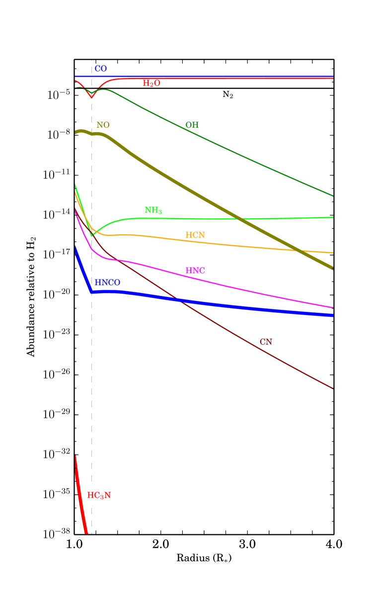
Figure 11: Thermodynamical chemical equilibrium model predictions for the innermost layers of an O-rich AGB CSE with characteristics presumably similar to those in OH 231.8$+$4.2 (§ 5). The spatial distribution of the N-bearing molecules detected in this work and other relevant species are plotted. The dashed vertical line denotes the boundary between the static and the dynamic atmosphere, at $\sim$1.2$R_{\star}$.

The spatial distribution of the molecular abundances near the star predicted by our TE chemistry model is shown in Fig. 11. In all cases, the model abundances are several orders of magnitude lower than those derived from the observations (Table 4). The largest model-data discrepancy is found for HC₃N, which is formed with an extremely marginal peak fractional abundance of $X$(HC₃N)$<$10^-32. NO is (after N₂) the most abundant N-compound in the hot photosphere, although the TE peak abundance is two orders of magnitude lower than observed in OH 231.8$+$4.2. We may safely conclude that the high abundances derived from the observations for these molecules cannot be explained as a result of equilibrium processes at the innermost parts of the envelope where, in contrast, abundant parent molecules, such as CO, N₂, and H₂O, are efficiently formed.

5.3 Chemical kinetics model

Our chemical kinetics model is based on that of Agúndez & Cernicharo (2006), which has been widely used to model the chemistry across the different envelope layers of the prototype C-rich star IRC 10216 (see also Agúndez et al., 2007; Agúndez et al., 2008; Agúndez et al., 2010) and, most recently, the O-rich YHG IRC+10420 (Quintana-Lacaci et al., 2013). The chemical network in our code includes gas-phase reactions, cosmic rays, and photoreactions with interstellar UV photons, but it does not incorporate reactions involving dust grains, X-rays, or shocks. Chemical reactions considered in this network are mainly obtained from the UMIST database (Woodall et al., 2007). The network has been updated with the latest kinetic rates and coefficients for HNCO (Quan et al., 2010). As mentioned in Sect. 5.2, HNCS has not been modelled because thermochemical parameters or reaction kinetic rates are not available for this molecule. Considering that oxygen is more abundant than sulphur (by a factor O/S$\sim$37; Table 6), we expect the HNCS abundance to be lower than that of its O-analogue, HNCO.

There are two major inputs to our chemical kinetics model, namely, the physical model of the envelope (models $a$ and $b$, respectively in § 5.1) and the initial abundances of the ‘parent’ species, formed in deeper layers, which are injected into the envelope. Once incorporated into the outflowing wind, these parent species become the basic ingredients for the formation of new (‘daughter’) molecules. The initial abundances of the parent species used in our model are given in Table 7. These abundances come from thermodynamical chemical equilibrium calculations and observations in the inner regions of O-rich envelopes (references are provided in this table). In the case of NH₃, which is a basic parent molecule for the formation of N-bearing species, we have adopted the value at the high end of the range of abundances observationally determined for a few O-rich CSEs, X(NH₃)$\sim$[0.2-3]$\times$10^-6 (Menten et al., 2010). We note that, as also pointed out by these authors, the formation of circumstellar NH₃ is particularly enigmatic since the observed abundances exceed the predictions from conventional chemical models by many orders of magnitude.

Our chemical kinetics model has been used first to investigate the formation of HNCO, HNCS, HC₃N, and NO in the intermediate/outer envelope of an O-rich AGB star similar to the slow central component of OH 231.8$+$4.2 (model $a$ described in § 5.1, see also Table 5). The spatial distribution of the model molecular abundances as a function of the distance to the centre are shown in Fig. 12. As the gas in the envelope expands, parent molecules start to be exposed to the interstellar UV radiation and photochemistry drives the formation of new species. Penetration of photons through deeper layers is gradually blocked by the dust extinction. At the very inner layers of the intermediate/outer envelope, parent species are preserved with their initial abundances, and at the very outermost layers, all molecules are finally fully dissociated (destroyed).

As seen in Fig. 12, the peak abundances of all the N-molecules detected in this work are significantly lower than observed, except for NO (by 3-4 orders of magnitude). The peak fractional abundance for NO predicted by the model, $X$(NO)$\sim$3$\times$10^-6, is in principle consistent with the average value measured in OH 231.8$+$4.2. According to our calculations, this molecule is expected to form rather efficiently in the winds of O-rich CSEs mainly via the gas-phase reaction

$$\mathrm{N+OH\longrightarrow NO+H}$$ (7)

and, therefore, NO should be common amongst O-rich evolved stars. Detection of NO emission lines is, however, hampered by the low dipole moment of this molecule ($\mu$=0.16 Debyes).

As derived from our model, the main chemical routes that would form HNCO and HC₃N in an O-rich CSE are

$$\mathrm{CN+OH\longrightarrow NCO+H}$$ (8)

$$\mathrm{H_{3}^{+}+NCO\longrightarrow HNCO^{+}+H_{2}}$$ (9)

$$\mathrm{HNCO^{+}+H_{2}\longrightarrow HNCOH^{+}+H}$$ (10)

$$\mathrm{HNCOH^{+}+e^{-}\longrightarrow HNCO+H}$$ (11)

and

$$\mathrm{CN+C_{2}H_{2}\longrightarrow HC_{3}N+H}.$$ (12)

However, the standard processes considered here are not sufficient to reproduce the abundances observed in the particular case of OH 231.8$+$4.2.

Table 7: Initial abundances relative to H₂ for representative elements and parent molecules used as input for the chemical kinetics models.

Species	Abundance	Reference
He	0.17	a
H2O	3.0$\times$10-4	b,TE
CO	3.0$\times$10-4	c,TE
CO2	3.0$\times$10-7	d
NH3	3.0$\times$10-6	e
N2	4.0$\times$10-5	TE
HCN	2.0$\times$10-7	f,g
H2S	7.0$\times$10-8	h
SO	9.3$\times$10-7	f
SiO	1.0$\times$10-6	i
SiS	2.7$\times$10-7	j

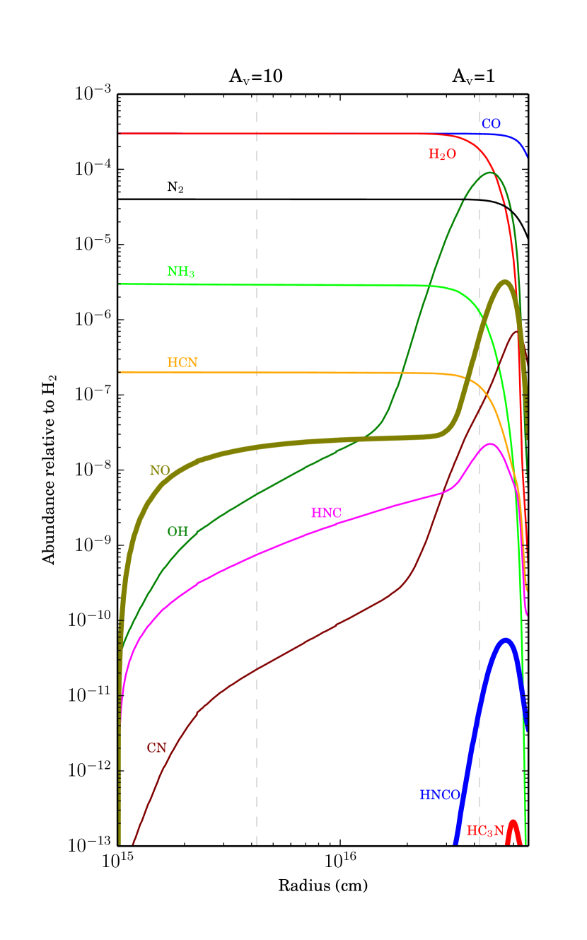
Figure 12: Chemical kinetics model predictions for the intermediate/outer layers of an O-rich AGB CSE with physical properties similar to those of the slow central parts of OH 231.8$+$4.2 (model input $a$, § 5 and Table 7). The species represented are as in Fig. 11.

We have investigated whether deeper penetration of interstellar UV radiation through the lobe walls of OH 231.8$+$4.2, which are on average more tenous than the central regions, can result in a significant production of HNCO and HC₃N, which could explain the observations. The input physical model for the lobe walls (a rectangular gas slab, model $b$) is described in Sect. 5.1. The total extinction through the lobe walls is $A_{V}$$\sim$2.3 mag, taking their thickness, mean H₂ number density, and the standard $n_{\mathrm{H_{2}}}$/$A_{v}$ conversion into account (Bohlin et al., 1978). The variation with time of the fractional abundances predicted by the model for a representative cell in the middle of the lobe walls ($A_{V}$$\sim$1 mag) are shown in Fig. 13.

As in the central nebular regions (model $a$), the abundances of HNCO (and probably HNCS) and HC₃N in the lobes never reach values comparable to those observationally determined. Except for NO, the abundances predicted in the lobes after $\sim$800 yr, which is the dynamical age of the molecular flow of OH 231.8$+$4.2, are lower than those expected in the slow central parts. We find that NO reaches a fractional abundance of $\sim$4$\times$10^-6 in $\sim$800 yr. This value is comparable to the average NO abundance deduced from the observations and to the value found in the slow central component (model $a$, Fig. 12).

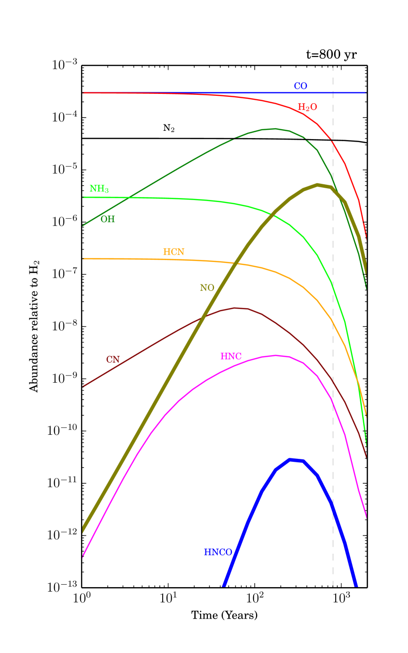
Figure 13: Evolution with time of the molecular fractional abundances predicted by our chemical kinetics model for a rectangular slab of gas (plane-parallel geometry) with physical properties similar to those of the walls of the hollow lobes of the molecular outflow of OH 231.8$+$4.2 (model input $b$, § 5). The model presented is for a representative gas cell in the middle of the lobe walls ($A_{V}$=1 mag). The species represented are as in Fig. 11 and 12, except for HC₃N, which has a predicted maximum abundance ($\approx$10^-19) well below the lower limit of the $y$-axis.

5.4 Enhanced N elemental abundance

We have considered whether an overabundance of the elemental nitrogen could result in fractional abundances of N-bearing compounds in better agreement with the observations. Such an elemental N-enrichment could result from hot bottom burning (HBB) process for stars with masses $\ga$3 $M_{\odot}$  and it has been proposed to explain the high abundance of NO deduced in the molecular envelope of the yellow hypergiant (YHG) star IRC$+$10420 (Quintana-Lacaci et al., 2013, and references therein).

As a first step, we ran our TE model again, increasing the elemental nitrogen abundance by a factor 40 – a larger enrichment factor is not expected (Boothroyd et al., 1993). In the inner layers of the envelope, our TE model shows that the N₂ fractional abundance increases proportionally, i.e.  also by a factor 40. Other N-bearing molecules, such as NH₃, HCN, NO, HNCO, and HC₃N, are less sensitive to the initial N-abundance, and they increase their abundances by a smaller factor, $\sim$5-10. As expected, given the very large discrepancy between TE model and data abundances, this factor is insufficient to explain the observations in OH 231.8$+$4.2.

As a second step, we ran our chemical kinetics model (case $a$) again but modified the initial abundances of relevant parent species (N₂, NH₃, and HCN) according to the TE predictions: N₂ in increased by a factor 40 and NH₃ and HCN by a factor 7 relative to the values in Table 7. Our TE calculations also show that these are the N-containing molecules that are most sensitive to the initial abundance of N. From our chemical kinetics model, we find that neither HNCO (and presumably HNCS) nor HC₃N experiment a significant variation, maximum abundance of HNCO is $\sim$8$\times$10^-10 and $\sim$8$\times$10^-13 for HC₃N, which are still low compared to the values derived from the observations. As NO concerns, we find a model peak abundance of $\sim$3$\times$10^-5 in the outer layers of the slow central component, which would be in excess of the value derived from the observations in OH 231.8$+$4.2. We therefore believe that a resonable enhancement of the elemental abundance of nitrogen, if it exists, would not reproduce the abundances of the N-molecules discussed by us satisfactorily. On the one hand, HNCO, HNCS, and HC₃N are underestimated, and on the other, NO (and maybe others, such as NH₃) would be significantly overestimated.

6 Discussion

Except maybe for NO, the relatively large abundances of the N-molecules detected in this work cannot be explained as thermodynamical chemical equilibrium or photodissociation products in the outflow of OH 231.8$+$4.2, even in the case of HNCO after considering IR pumping effects (§ 4.2, Appendix A). In principle, the inability of the model to reproduce the observed abundances of HNCO, HNCS, and HC₃N could be attributed to the simplicity of the physico-chemical scenario adopted, for example, to the lack of certain molecule formation routes (e.g. involving dust grains). However, if these were the main reasons for the model-data discrepancies in OH 231.8$+$4.2 (and provided that these unknown chemical routes prove to be an efficient way of producing HNCO, HNCS, and HC₃N in O-rich environments, which remains to be seen), then these molecules should be present with comparable abundances in other O-rich envelopes of similar characteristics.

These molecules have been searched for but not detected by our team (and others) in two of the strongest molecular emitters and best studied O-rich envelopes: the AGB star IK Tau (Velilla et al., in prep) and the red supergiant VY CMa (Quintana-Lacaci et al., in prep). In these objects, NO is detected with a fractional abundance of $X$(NO)$\approx$10^-7, in agreement with the model predictions, but only upper limits are obtained for the rest of the N molecules discussed here, $\la$10^-9-$\la$10^-10. The upper limits estimated for IK Tau and VY CMa are consistent with the low abundances predicted by the models, which suggests that the physico-chemical scenario used by us is an acceptable representation of a standard O-rich AGB CSE. We recall that the notable chemical differences between OH 231.8$+$4.2 and other O-rich AGB CSE are widely recognized and are not restricted to the N-molecules detected here but affect most of the species identified in this object, including C-, N-, and S-containing ones such as HCN, H₂CO, H₂S, SO, SO₂, which are undetected or detected with much lower abundances in ‘normal’ O-rich AGB CSE, as pointed out by previous works (§ 1).

In principle, there is no reason to suspect a particularly intense interstellar UV radiation field or peculiar dust properties or content that could (or not) account for the unique, rich chemistry of OH 231.8$+$4.2 compared to its O-rich relatives. The main difference between OH 231.8$+$4.2 and ‘normal’ O-rich AGB CSEs is the presence of a fast ($\sim$400 km s^-1) accelerated outflow in the former. Given the formation history of such an outflow, possibly as the result of a sudden jet+‘AGB CSE’ interaction $\sim$800 yr ago (§ 1), fast shocks have probably played a major role not only in the physics but also in the chemistry of OH 231.8$+$4.2. Molecules are expected to be initially destroyed by the high-speed axial shocks produced in the jet+’AGB CSE’ interaction (e.g. Neufeld, 1990). At present, the shocked material has cooled down sufficiently to allow molecule reformation, which probably happened very quickly, in less than $\sim$150 yr, under non-equilibrium conditions. Moreover, additional atoms (Si, S, etc.) may have been extracted by the shocks from the dust grains and released into the gas phase (Morris et al., 1987; Lindqvist et al., 1992), altering the proportions of the different elements available for molecule regeneration in the post-shocked gas. Both non-equlibrium conditions and non-standard elemental proportions in the post-shocked gas are crucial factors determining the abundances of the second-generation molecules in OH 231.8$+$4.2.

Shocks could also have been decisive in defining the chemistry of the slow central parts of the envelope around OH 231.8$+$4.2. As already pointed by, for example, Lindqvist et al. (1992), the maximum expansion velocities measured towards the central nebular regions, $V_{\mathrm{exp}}$$\sim$35 km s^-1, are higher than for normal OH/IR stars, which indicates that some acceleration is likely to have occurred. In fact, it may be possible for shocks developed in the jet+‘AGB CSE’ interaction to move sideways and backward (with moderate velocities lower than those reached along the jet axis) compressing the gas in the equatorial plane and shaping the central, torus-like structure of OH 231.8$+$4.2. Although these moderate-velocity ($\la$40 km s^-1) shocks are not expected to destroy molecules (at least not fully), the compression and heating of these equatorial regions would result in a profound chemical mutation with respect to normal unperturbed AGB CSEs (for example, activating certain endothermic reactions, or exothermic reactions with barriers, otherwise forbidden).

7 Summary and conclusions

We have reported the first detection of the N-bearing molecules HNCO, HNCS, HC₃N, and NO in the circumstellar envelope of the O-rich evolved star OH 231.8$+$4.2 based on single-dish observations with the IRAM-30 m telescope. HNCO and HNCS are first detections in circumstellar envelopes; HC₃N is a first detection in an O-rich environment; NO is a first detection in a CSE around a low-to-intermediate-mass, evolved star. From the observed profiles, we deduce the presence of these species in the slow central parts of the nebula, as well as at the base of the fast bipolar lobes.

The intense, low-velocity components of the HNCO $K_{\rm a}$=0, HNCS, and HC₃N profiles have similar widths (FWHM$\sim$20-30 km s^-1) and velocity peaks ($V_{\mathrm{LSR}}$$\sim$28-29 km s^-1). Previous SO emission mapping (Sánchez Contreras et al., 2000b) shows the presence of an equatorial expanding disk or torus around the central star that produces double-peaked (at $V_{\mathrm{LSR}}$=28 and 40 km s^-1) spectral profiles in many SO transitions (and also in other molecules). The coincident peak velocity of HNCO, HNCS, and HC₃N transitions with the blue peak of the disk/torus feature suggests that part of the low-velocity emission from these molecules may arise at this equatorial structure. The HNCO $K_{\rm a}$=1 transitions are narrower, with FWHM$\sim$13 km s^-1, and may arise in regions closer in to the central source.

The profiles of the NO lines are broader (FWHM$\sim$40-50 km s^-1) and are centred on somewhat redder velocities $V_{\mathrm{LSR}}$$\sim$40 km s^-1. As explained in Sect. 3, this is not only due to the hyperfine structure of the NO transitions, but it also indicates that a significant part of the NO emission is produced in regions with high expansion velocities; in particular, the contribution to the emission from clump I4 at the base of the southern lobe is notable. Broad profiles (FWHM$\sim$40-90 km s^-1) are also found for mm-wave transitions of HCO⁺ (Sánchez Contreras et al., 2000b) and other molecular ions recently discovered by us in OH 231.8$+$4.2 (Sánchez Contreras et al. 2014, in prep.). This suggests a similar spatial distribution of these species with enhanced abundances in the high-velocity gas relative to the low-velocity nebular component at the centre.

We derived typical rotational temperatures of $\sim$15-30 K, in agreement with previous estimates of the kinetic temperature in the CO flow (Alcolea et al., 2001). Non-LTE effects are expected to be moderate, given the relatively high densities of the dominant emitting regions ($\ga$10⁵  cm^-3). Nevertheless, in the case of HC₃N, moderate sub-thermal excitation is possible in the most tenuous parts of the outflow, and somewhat higher temperatures of $\sim$45 to 55 K cannot be ruled out. Adopting a characteristic size of the emitting nebula of $\sim$4″$\times$12″, we obtained column densities of $N_{\mathrm{tot}}$(¹³CO)$\sim$3$\times$10¹⁷  cm^-2, $N_{\mathrm{tot}}$(HNCO)$\sim$6$\times$10¹⁴  cm^-2, $N_{\mathrm{tot}}$(HNCS)$\sim$7$\times$10¹³  cm^-2, $N_{\mathrm{tot}}$(HC₃N)$\sim$3$\times$10¹³  cm^-2, and $N_{\mathrm{tot}}$(NO)$\sim$9$\times$10¹⁵  cm^-2.

The beam-averaged fractional abundances in OH 231.8$+$4.2 obtained are (in decreasing order) $X$(NO)$\sim$[1-2]$\times$10^-6, $X$(HNCO)$\sim$[0.8-1]$\times$10^-7, $X$(HNCS)=[0.9-1]$\times$10^-8, and $X$(HC₃N)=[5-7]$\times$10^-9. We note the large abundance of NO, which is comparable to that of, e.g., SO and SO₂ (already known to be dominant in OH 231.8$+$4.2). Our measurement implies that NO is one of the most abundant N-containing molecule in this object. Also remarkable is the relatively large abundance of HNCO, closely following that of major carriers of carbon in OH 231.8$+$4.2, apart from CO and ¹³CO, such as HCN, H₂CO, and CS, and comparable to and even larger than that of HNC and HCO⁺ (Morris et al., 1987; Lindqvist et al., 1992; Sánchez Contreras et al., 1997, 2000b; Velilla Prieto et al., 2013; Sánchez Contreras et al., 2014).

We modelled thermodynamical equilibrium and non-equilibrium kinetically driven chemistry to investigate the production of HNCO, HC₃N, and NO in OH 231.8$+$4.2. HNCS cannot be modelled because of the lack of thermochemical parameters and reactions rates. We modelled the slow central component and the lobe walls separately.

We found that none of the molecules HNCO, HC₃N, or NO are formed in significant amounts in the vicinity of the AGB star (up to $\sim$4$R_{\star}$), where thermodynamical equilibrium conditions prevail (Fig. 11). In these regions, the vast majority of N atoms are locked in N₂, followed by NO.

In the intermediate/outer layers of the slow central component of the envelope (from $\sim$10¹⁵ to $\sim$10¹⁷   cm^-), the model fails to reproduce the large abundances observed in OH 231.8$+$4.2, except for NO (Fig. 12). The model-data discrepancies cannot be explained by a reasonable enhancement of the elemental nitrogen abundance (as a result of HBB processes).

In the lobes, our chemistry model indicates that the only molecule that reaches fractional abundances comparable to the values observationally determined is NO. For HNCO (and probably HNCS) and HC₃N, the model abundances in the lobes are more than five orders of magnitude lower than the observed average values.

Based on this and previous works, the rich chemistry of OH 231.8$+$4.2, which is unparalleled amongst AGB and post-AGB envelopes, is corroborated. New detection of HNCO, HNCS, HC₃N, and NO add to the list of N-bearing molecules present in its molecular outflow with high abundances. This could be the best example of a shocked environment around an evolved star, and OH 231.8$+$4.2 therefore stands out as a reference target for studying non-equilibrium, shock-induced chemical processes in oxygen-rich environments.

Appendix A Non-LTE effects on the population diagrams of HNCO, HNCS, HC₃N, and NO.

The population diagram method is a common tool for deriving physical gas conditions from molecular line observations (see Goldsmith & Langer, 1999, for a classic reference). It relies on two major assumptions: $i$) optically thin emission and $ii$) LTE conditions. The latter assumption (LTE) implies that the populations of all levels are described by the Boltzmann distribution with a unique rotational temperature, $T_{\mathrm{rot}}$, which is equal to the kinetic temperature of the gas ($T_{\mathrm{kin}}$=$T_{\mathrm{rot}}$). In this case, for a given molecule and a series of transitions $u\rightarrow l$, a plot of the natural logarithm of the upper state column density per statistical weight ($N_{u}/g_{u}$) versus the energy above the ground ($E_{\mathrm{u}}$), the so-called population diagram, will yield a straight line with a slope 1/$T_{\mathrm{rot}}$.

Goldsmith & Langer (1999) have numerically investigated how the optical depth and deviations from LTE affect the temperature and column density derived using the population diagram technique for two molecules: HC₃N and CH₃OH. In this appendix, we perform a similar analysis for HNCO, HNCS, HC₃N, and NO, but in this case, we focus on non-LTE excitation effects since the lines detected in OH 231.8$+$4.2 are optically thin. (For HC₃N we compared our results, analysing both optical depth and non-LTE excitation effects, with those by Goldsmith & Langer (1999) and found an excellent agreement.)

In low-density regions, LTE may not be a valid approximation, and therefore, the level populations, which may not longer be described well by the Boltzmann distribution, have to be numerically computed by solving the statistical equilibrium and radiation transport equations. The excitation analysis presented in this Appendix has been done using MADEX (Molecular and Atomic Database and EXcitation code, Cernicharo, 2012). This is a code that solves the molecular excitation (including collisional and radiative excitation mechanisms) and radiation transfer problem under the large velocity gradient (LVG) formalism. It contains up-to-date spectroscopy (rest frequencies, level energies, line strength/Einstein coefficients, etc.) and collisional rates available from the literature for more than 5000 different molecular and atomic entries including isotopologues and vibrationally excited states. MADEX computes molecule-H₂ collisional rates from those available in the literature by adopting other collision partners, such as He or para-$H_{2}$. MADEX also evaluates the partition function of the molecule (using a large enough number of levels to obtain accurate values of the partition function even at high temperatures) and predicts the emergent spectra.

To examine what happens if some or all of the transitions of HNCO, HNCS, HC₃N, and NO are not thermalized, we computed the level populations for a range of densities, $n_{\mathrm{H_{2}}}$, and a given input value of $T_{\mathrm{kin}}$ and $N_{\mathrm{tot}}$ for each molecule. The adopted values of $T_{\mathrm{kin}}$ and $N_{\mathrm{tot}}$ are similar to those obtained from the LTE analysis (§ 4.1). We assumed a linear velocity gradient d$(\ln V)$/d$(\ln r)$=1 and typical line widths of FWHM=20-40 km s^-1, as observed towards OH 231.8$+$4.2 (§ 1 and 3). The resulting population diagrams based on our non-LTE excitation calculations, including the LTE theoretical points, are shown in Fig. 14.

For HNCO we used collisional rates from Green (1986), computed for the lowest 164 levels at temperatures from 30 to 350 K. For the non-LTE analysis, we considered rotational levels in the ground vibrational state ($v$=0) up to $J_{\rm max}$=18 for both the $K_{\mathrm{a}}$=0 and $K_{\mathrm{a}}$=1 ladder transitions (and also up to $K_{\mathrm{a}}$=4, which has been included in the calculations). This implies a maximum upper state energy of 830 K. As shown in Fig. 14 (top left box), for the lowest density models ($n_{\mathrm{H_{2}}}$=10⁵ cm^-3), there is a notable separation between the $K_{\mathrm{a}}$=0 and $K_{\mathrm{a}}$=1 ladders, which follow two straight lines with different slopes. The slope of the $K_{\mathrm{a}}$=0 ladder implies a rotational temperature of $T_{\mathrm{rot}}$$\sim$16 K, which is lower than the real input kinetic temperature (sub-thermal excitation), while the slope of the $K_{\mathrm{a}}$=1 ladder implies a rotational temperature of $T_{\mathrm{rot}}$$\sim$30 K. The $y$-offset between the two $K_{\mathrm{a}}$ ladders decreases as the density increases, until they merge in a single line at densities $n_{\mathrm{H_{2}}}$$\ga$10⁸ cm^-3, with $T_{\mathrm{rot}}$=$T_{\mathrm{kin}}$.

Figure 14: Population diagrams of HNCO, HNCS, HC₃N, and NO for a range of molecular hydrogen densities ($n_{\mathrm{H_{2}}}$, bottom left corner) and a given input value for the kinetic temperature and total column density ($T_{\mathrm{kin}}$ and $N_{\mathrm{tot}}$; top right corner); the dotted line connects the LTE points. Only the transitions detected in this work are represented in this diagram (Table 3). For HNCO, the transitions within the $K_{\mathrm{a}}$=0 and $K_{\mathrm{a}}$=1 ladders are indicated by empty and filled symbols, respectively. For NO, we plot the three hyperfine components with the highest values of the Einstein coefficient (A_ul) for each of the $\Pi^{-}$ and $\Pi^{+}$ doublets at 250 and 350  GHz (i.e. at $E_{\mathrm{u}}$=19.2 and 36.1 K), the three hyperfine components with the largest A_ul of the $\Pi^{+}$ band at 150  GHz (i.e. at $E_{\mathrm{u}}$=7.2 K) and the $\Pi^{-}$(3/2,3/2)-(1/2,1/2) line, which is spectrally isolated in our data, at 150 GHz ($E_{\mathrm{u}}$=7.2 K). These calculations have been done with a LVG radiative transfer code (MADEX) – see text in this appendix.

Collisional rates are not available for HNCS, therefore we used those of HNCO after applying the standard reduced mass correction. As for HNCO, we included rotational levels of up to $J_{\rm max}$=18 (within the $K_{\mathrm{a}}$=0, 1, and 2 ladders), which implies maximum upper state energies of $E_{\mathrm{u}}$$\sim$355 K. As expected, deviations from LTE affect the population diagram of HNCS similarly to HNCO. In the case of HNCS, only the $K_{\mathrm{a}}$=0 ladder has been plotted since these are the only ones detected. For the lowest density model, $n_{\mathrm{H_{2}}}$=10⁴  cm^-3, the inferred values of $T_{\mathrm{rot}}$$\sim$10-12 K deviate significantly from the real input values ($T_{\mathrm{kin}}$=25 K).

Collisional rates for HC₃N are from Wernli et al. (2007), which include 51 levels and are computed for temperatures between 5 K and 100 K. Collisional rates for NO are adopted from Kłos et al. (2008), computed for 98 rotational levels and temperatures between 10 and 500 K. The highest rotational levels included in our non-LTE excitation calculations for HC₃N an NO are $J_{\rm max}$=30 ($E_{\mathrm{u}}$^max$\sim$200 K) and $J_{\rm max}$=13/2 ($E_{\mathrm{u}}$^max$\sim$300 K), respectively. The resulting non-LTE models for HC₃N and NO (Fig. 14), as for the other species, clearly show steeper slopes ($T_{\mathrm{rot}}$$<$$T_{\mathrm{kin}}$) for the lowest density models. Another effect of non-LTE excitation is that the different level populations cannot be described by a unique rotational temperature, which translates into a different slope for the low-$J$ and high-$J$ levels in the population diagram. This effect is most notable for HC₃N: the temperatures implied are $T_{\mathrm{rot}}$$\sim$5 K for the three lowest-$J$ levels and $T_{\mathrm{rot}}$$\sim$7 K for the four highest-$J$ levels. The HC₃N column densities that one would derive using low-$J$ or high-$J$ levels are also different, in particular, $N_{\mathrm{tot}}$(low-$J$)=3.3$\times$10¹³  cm^-3 $>$$N_{\mathrm{tot}}$=3.0$\times$10¹³  cm^-3 $>$ $N_{\mathrm{tot}}$(high-$J$)=7.2$\times$10¹²  cm^-3. In the lowest density model of NO, the implied $T_{\mathrm{rot}}$ ($<$$T_{\mathrm{kin}}$=26 K) does not vary appreciably across the different levels (less than 6%).

For all molecules, at the highest densities considered, the populations of the levels considered are thermalized or very close to thermalization, and the non-LTE and LTE predictions converge. In both cases, the data points in the population diagram can be satisfactorily fit by a straight line with $T_{\mathrm{rot}}$=$T_{\mathrm{kin}}$. We consider of interest to provide a summary with the range of critical densities for the transitions analysed in this work. These are for a representative temperature of 25 K, which is common in the dominant emitting components of AGB CSEs and PPNs (Bujarrabal et al., 2001). For HNCO the critical densities are in the range of $n_{\mathrm{crit}}$=[4$\times$10⁵-1$\times$10⁷] cm^-3 for the $K_{\mathrm{a}}$=0 transitions, and $n_{\mathrm{crit}}$=[1$\times$10⁶-1$\times$10⁷] cm^-3 for the $K_{\mathrm{a}}$=1 transitions. For HNCS, HC₃N, and NO, the critical densities are $n_{\mathrm{crit}}$=[5$\times$10⁵-2$\times$10⁶] cm^-3, $n_{\mathrm{crit}}$=[1$\times$10⁶-3$\times$10⁶] cm^-3, and $n_{\mathrm{crit}}$=[2$\times$10⁴-2$\times$10⁶], respectively. In all these cases, the lowest value of $n_{\mathrm{crit}}$ in the ranges given above corresponds to the lowest-$J$ and/or lowest-E_u transition.

Finally, we briefly comment on the possible effect of the pumping of the rotational levels of HNCO by the infrared (IR) photons emitted by the star and the central dust region (see e.g. Kuan & Snyder, 1996). This IR emission would cause the radiative pumping of levels inside the ground vibrational state and the vibrationally excited states of HNCO. The latter would eventually produce a fluorescence effect between the ground state and the six vibrational modes of HNCO. The radiative pumping inside the rotational levels of the ground state alone was found to be dominant in the HNCO excitation in Sgr B2 (Churchwell et al., 1986). In this region, the typical densities are relatively low, n(H₂)$\sim$10⁴ cm^-3, but the central source is optically thick at 100 $\mu$m and extended. The IR pumping through vibrationally excited states, has also noticeable effects in the emerging intensities of some rotational lines for certain molecules like H₂O IRC+10216 (Agúndez & Cernicharo, 2006). Recently, it has been pointed out that the time variability of the IR pumping can produce intensity variations in the high rotational lines of abundant molecules in the envelopes of Mira-type stars, such as CCH towards IRC+10216 (Cernicharo et al., 2014). Thus, to summarize, transitions with high upper level energies or those that are severely underexcited by collisions could be more sensitive to IR pumping. When HNCO levels were populated mainly by IR radiation, the column density implied by the rotational diagram method could be different than the true value; the rotational temperature would also be different than the gas kinetic temperature (but see next paragraph).

Our previous discussion of the excitation state of the observed lines of HNCO shows that they are practically thermalized to the temperatures expected in the studied nebula. The population diagram of HNCO (Fig. 9) covers a wide range of upper energies, and it clearly shows a single slope for both the K_a=0 and K_a=1 transitions. This should imply that the line intensities are described well by one rotational temperaure, so that the column density and the derived abundance should be close to the true value. Also, the range of derived kinetic temperatures is consistent with previous estimations of the rotational temperatures and the kinetic temperature in the CO flow (see e.g. Guilloteau et al., 1986; Morris et al., 1987; Alcolea et al., 2001). Finally, the bulk of the emission of HNCO (§ 3) arises from the central dense region of the CSE (I3) and the base of the southern lobe (I4). These regions are characterized by densities of n(H₂)$\geq$10⁶-10⁷ cm^-3 in the central region and n(H₂)$\geq$10⁵ cm^-3 in the lobes (Alcolea et al., 2001; Bujarrabal et al., 2002). This leads to densities close or higher than the critical densities for HNCO K_a=0 and K_a=1 transitions. Therefore, the effects of vibrational cascades should be minor in our case, but we cannot rule out uncertainties in the abundance of HNCO less than a factor 2-5. On the other hand, we have seen that the excitation via the various vibrational states is extremely complex for these relatively heavy molecules. A detailed study of these intricate phenomena is obviously beyond the scope of this paper.

Appendix B Comparison with other astrophysical environments

B.1 HNCO

Isocyanic acid has been detected in different environments with a variety of physical conditions, including SgrB2 (Snyder & Buhl, 1972), the Taurus Molecular Cloud TMC-1 (Brown, 1981), external galaxies (Nguyen-Q-Rieu et al., 1991), the shocked-outflow of the young stellar object L1157 (Rodríguez-Fernández et al., 2010), hot cores (Churchwell et al., 1986; Martín et al., 2008), translucent clouds (Turner et al., 1999), etc. Nevertheless, prior to this work, HNCO was not detected in any CSE around evolved stars, either oxygen or carbon rich.

Formation of HNCO through gas-phase and grain surface chemistry from different chemical pathways has been studied by several authors (Iglesias, 1977; Turner et al., 1999; Zinchenko et al., 2000; Garrod et al., 2008; Marcelino et al., 2010; Quan et al., 2010). This molecule was first proposed as a high density tracer (Jackson et al., 1984) and, more recently, a shock tracer (Rodríguez-Fernández et al., 2010, and references therein).

The fractional abundance of HNCO varies somewhat in different sources, typically within the range $\approx$10^-10 -10^-9. The highest fractional abundance (relative to H₂) of HNCO has been measured towards the shocked region of the L1157 outflow, L1157-B2, where $X$(HNCO)$\sim$9.6$\times\,10^{-8}$ (Rodríguez-Fernández et al., 2010). Interestingly, this value of the abundance is comparable to what is estimated towards OH 231.8$+$4.2.

B.2 HNCS

Isothiocyanic acid was first detected in SgrB2 (Frerking et al., 1979) and has been recently observed in TMC-1 (Adande et al., 2010). Detection of HNCS in a circumstellar envelope has not been reported previously to this work.

The formation of HNCS in the cold core TMC-1 and the hot core in SgrB2 has been studied theoretically through gas-phase, ion-molecule chemistry and grain surface reactions (Adande et al., 2010). Prior to this work, the highest abundance of HNCS had been found towards SgrB2 and TMC-1, with a value of $\approx\,10^{-11}$. In OH 231.8$+$4.2  we derive a fractional abundance of HNCS that is about 1000 times higher.

B.3 HC₃N

Cyanoacetylene is detected in assorted environments, including SgrB2 (Turner, 1971), H II regions, dark clouds (Morris et al., 1976), the Orion molecular cloud (Goldsmith et al., 1982), the Perseus globules (Bachiller & Cernicharo, 1986), in the Taurus molecular clouds (Cernicharo et al., 1984), protoplanetary disks (Chapillon et al., 2012), etc. HC₃N is also detected in several C-rich CSEs, including the well-known AGB star IRC$+$10216 and the protoplanetary nebula CRL 618 (e.g. Morris et al., 1975; Bujarrabal et al., 1994; Audinos et al., 1994; Cernicharo et al., 2000; Pardo et al., 2004); however, this molecule has not been identified before in an O-rich CSE.

HC₃N is considered to be a high density tracer (Morris et al., 1976) and in CSEs, particularly in IRC$+$10216, it is distributed in a hollow spherical shell around the central star, which is a major product of photodissociation in the outer parts of the envelope (Audinos et al., 1994). The observed abundance in IRC$+$10216 is $X$(HC₃N)$\sim$1$\times$10^-6 agrees with theoretical predictions in C-rich CSEs (Agúndez et al., 2010). We infer $X$(HC₃N)$\sim$7$\times\,10^{-9}$ towards OH 231.8$+$4.2. This value is much lower than in IRC$+$10216 by virtue of the O-rich vs. C-rich nature of both sources.

B.4 NO

Nitric oxide has been previously detected in several astrophysical environments, including molecular clouds (Gerin et al., 1992), SgrB2 (Halfen et al., 2001), and pre-protostellar cores (Akyilmaz et al., 2007). Recently, NO has been detected for the first time in the CSE around the yellow hypergiant (YHG) IRC$+$10420, which is a massive ($\sim$50 $M_{\odot}$) evolved star with a N-rich chemistry (Quintana-Lacaci et al., 2013), with a fractional abundance of $X$(NO)$\approx$10^-5.

Chemical models presented by Quintana-Lacaci et al. (2013) in IRC$+$10420 predict that indeed NO forms very efficiently by photochemistry (mainly through the reaction N + OH $\longrightarrow$ NO + H) in the outer circumstellar layers, where it reaches a maximum abundance of $\approx$10^-6. In the case of IRC$+$10240, nitrogen enrichment due to hot bottom burning has been proposed to explain the NO abundance observed, which is larger by a factor 10 than predicted by these models adopting the solar nitrogen abundance.

Appendix C Ionization and dissociation sources in our chemistry models

The sources of ionization and dissociation adopted in our model are cosmic rays and the interstellar ultraviolet radiation field. The cosmic-ray ionization rate adopted is 1.2$\times$10^-17 s^-1 (Dalgarno, 2006). The intensity of the UV field assumed is the Draine field (X) or Go=1.7 in units of the Habing field (Go=1.6$\times$10⁻³ erg s^-1 cm^-2; Habing, 1968, Draine & Salpeter, 1978). The ISM UV field illuminates the nebula externally.

We also evaluated two possible additional sources of internal ionization and dissociation in OH 231.8$+$4.2: 1) the UV radiation by the A0 main sequence companion of the primary AGB star (QX Pup) at the nucleus of the nebula, and 2) the high-energy radiation generated by the cooling of hot gas behind the fast shock fronts ahead of the lobe tips (Sect. 1). In both cases, the effect on the chemistry is not expected to be predominant and has not been considered in our model.

First, the UV radiation field emitted by the $\sim$10 000 K main-sequence companion cannot penetrate very deep through the dense dusty wind of the AGB mass-losing star except, maybe, along the direction of the lobes owing to the lower extinction by dust along the outflow cavities (of the order of $A_{V}$$\sim$1 mag; Sánchez Contreras et al., 2004). However, there is observational evidence against the presence of a substantial amount of ionized or atomic gas in the stellar vicinity, hence against the existence of an intense stellar UV field that could have a noticeable effect on the chemistry in the inner regions of the lobes: ($i$) the lack of H_α emission (or any other recombination or forbidden lines in the optical) from the nucleus of OH 231.8$+$4.2 rules out an emergent ionized region around the star (Cohen et al., 1985; Reipurth, 1987; Sánchez Contreras et al., 2000a, 2004); and ($ii$) the lack of low-excitation atomic emission lines in the far-infrared, e.g. [O I] emission at 63.2 and 145.5$\mu$m (unpublished Herschel archive data) indicates the absence of a photodissociation region (PDR) in the nebula centre. Moreover, considering the temperature and luminosity of the warm companion ($\sim$10 000K and $\sim$5-30$L_{\odot}$; Sánchez Contreras et al., 2004), it can be demonstrated that the stellar UV flux that reaches to a point located at the inner edges of the lobes ($\sim$4″ from the star) with a visual extinction of A_V=1.0 mag, would be smaller than, or at most comparable to, the ISM UV field. Therefore, including the stellar UV radiation as a source of internal illumination of the lobe walls in the model will yield very similar results (and even smaller molecular abundances for ‘daughter’ species) to those obtained assuming external illumination by the ISM UV field.

Second, the shocks that are currently active in OH 231.8$+$4.2 are those traced by H_α emission, which arises in two bubble-like structures of shock-excited gas surrounding the molecular outflow (Reipurth, 1987; Sánchez Contreras et al., 2000a; Bujarrabal et al., 2002). These fast shocks may have been generated by interaction between the dense, fast molecular outflow and the tenuous ambient material. The characteristics of the exciting shocks have been studied in detail by Sánchez Contreras et al. (2000a). In particular, these authors compare the relative intensities of the different optical lines observed with the diagnostic diagrams by Dopita & Sutherland (1995), which can distinguish between shocks with or without a photoionized preshock region. These diagrams not only confirm the shock nature of the emission but also indicate that the emission from a photoionized precursor region is either weak or absent. We note, moreover, that even in the improbable case that sufficiently intense UV radiation from the current shocks is produced, its effect on the chemistry will be almost exclusively limited to the outflow regions immediately behind the shock fronts, that is, the molecular clumps at the very end of the lobes of OH 231.8$+$4.2. However, given the beam size of our observations (Fig.1), the contribution of these molecular clumps to the total emission by the N-bearing molecules reported in this work is insignificant.