Statistical Modeling and Probabilistic Analysis of Cellular Networks with Determinantal Point Processes

Abstract

Although the Poisson point process (PPP) has been widely used to model base station (BS) locations in cellular networks, it is an idealized model that neglects the spatial correlation among BSs. The present paper proposes the use of determinantal point process (DPP) to take into account these correlations; in particular the repulsiveness among macro base station locations. DPPs are demonstrated to be analytically tractable by leveraging several unique computational properties. Specifically, we show that the empty space function, the nearest neighbor function, the mean interference and the signal-to-interference ratio (SIR) distribution have explicit analytical representations and can be numerically evaluated for cellular networks with DPP configured BSs. In addition, the modeling accuracy of DPPs is investigated by fitting three DPP models to real BS location data sets from two major U.S. cities. Using hypothesis testing for various performance metrics of interest, we show that these fitted DPPs are significantly more accurate than popular choices such as the PPP and the perturbed hexagonal grid model.

I Introduction

Historically, cellular base stations have been modeled by the deterministic grid-based model, especially the hexagonal grid. However, the increasingly dense capacity-driven deployment of BSs, along with other topological and demographic factors, have made cellular BS deployments more organic and irregular. Therefore, random spatial models, in particular the PPP, have been widely adopted to analyze cellular networks using stochastic geometry [2, 3, 4, 5, 6, 7, 8, 9, 10, 11]. However, since no two macro base stations are deployed arbitrarily close to each other, the PPP assumption for the BS locations fails to model the underlying repulsion among macro BSs and generally gives a pessimistic signal-to-interference-plus-noise ratio (SINR) distribution [2]. In this paper, we propose to use DPPs [12] to model the macro BS locations. We demonstrate the analytical tractability of the proposed model and present statistical evidence to validate the accuracy of DPPs in modeling BS deployments.

I-A Related Works

Cellular network performance metrics, such as the coverage probability and achievable rate, strongly depend on the spatial configuration of BSs. PPPs have become increasingly popular to model cellular BSs not only because they can describe highly irregular placements, but also because they allow the use of powerful tools from stochastic geometry and are amenable to tractable analysis [2]. While cellular networks with PPP distributed BSs have been studied in early works such as [13, 14, 15], the coverage probability and average Shannon rate were derived only recently in [2]. The analysis of cellular networks with PPP distributed BSs has been widely extended to other network scenarios, including heterogeneous cellular networks (HetNets) [3, 4, 5, 6, 7], MIMO cellular networks [8, 9], and MIMO HetNets [8, 10, 11].

Real (macro) BS deployments exhibit “repulsion” between the BSs, which means that macro BSs are typically distributed more regularly than the realization of a PPP. Although the statistics of the propagation losses between a typical user and the BSs converge to that of a Poisson network model under i.i.d. shadowing with large variance [16], these assumptions are quite restrictive and may not always hold in practice. Therefore, several recent research efforts have been devoted to investigating more accurate point process models for representing BS deployments. One class of such point processes is the Gibbs point process [17, 18, 19]. Gibbs models were validated to be statistically similar to real BS deployments using SIR distribution and Voronoi cell area distribution [17]. The Strauss process, which is an important class of Gibbs processes, can also provide accurate statistical fit to real BS deployments [18, 19]. By contrast, the PPP and the grid models were demonstrated to be less accurate models for real BS deployments [17, 18]. A significant limitation of Gibbs processes is their lack of tractability, since their probability generating functional is generally unknown [18]. Therefore, point processes that are both tractable and accurate in modeling real BS deployments are desirable.

For several reasons, determinantal point processes (DPPs) are a promising class of point processes to model cellular BS deployments. First, DPPs have soft and adaptable repulsiveness [20]. Second, there are quite effective statistical inference tools for DPPs [12, 21]. Third, many stationary DPPs can be easily simulated [21, 22, 23]. Fourth, DPPs have many attractive mathematical properties, which can be used for the analysis of cellular network performance [24, 25].

The Ginibre point process, which is a type of DPP, has been recently proposed as a possible model for cellular BSs. Closed-form expressions of the coverage probability and the mean data rate were derived for Ginibre single-tier cellular networks in [25], and heterogeneous cellular networks in [26]. In [27], several spatial descriptive statistics and the coverage probability were derived for Ginibre single-tier networks. These results were empirically validated by comparing to real BS deployments. That being said, the modeling accuracy and analytical tractability of using general DPPs to model cellular BS deployments are still largely unexplored.

I-B Contributions

In this work, we derive several key performance metrics in cellular networks with DPP configured BSs for the first time. Then we use statistical methods to show that DPPs indeed accurately model cellular BSs. Finally, we describe the gains provided by the use of DPPs for the performance evaluation of cellular networks. The main contributions of this paper are now summarized.

DPPs are tractable models to analyze cellular networks: We summarize three key computational properties of the DPPs, and derive the Laplace functional of the DPPs and independently marked DPPs for functions satisfying certain conditions. Based on these computational properties, we analytically derive and numerically evaluate several performance metrics, including the empty space function, nearest neighbor function, mean interference and SIR distribution. The Quasi-Monte Carlo integration method is used for efficient evaluation of the derived empty space function, nearest neighbor function, and mean interference. Finally, the SIR distribution under the nearest BS association scheme is derived, and a close approximation is proposed for efficient numerical evaluation in the high SIR regime.

DPPs are accurate models for macro BS deployments: We fit three stationary DPP models—the Gauss, Cauchy and Generalized Gamma DPP—to real macro BS deployments from two major U.S. cities, and show that these DPP models are generally accurate in terms of spatial descriptive statistics and coverage probability. We find that the Generalized Gamma DPP provides the best fit to real BS deployments in terms of coverage probability, but is generally less tractable. In contrast, the Gauss DPP model also provides a reasonable fit while offering better mathematical tractability. Compared to other DPP models, the fitted Cauchy DPP provides the least precise results in terms of coverage probability. We also show that the fitted Generalized Gamma DPP is the most repulsive while the fitted Cauchy DPP is the least repulsive.

DPPs outperform the PPPs to predict key performance metrics in cellular networks: By combining the analytical, numerical and statistical results, we show that DPPs are more accurate than PPPs to model BS deployments in terms of the empty space function, the nearest neighbor function, the mean interference and most importantly, the coverage probability.

II Mathematical Preliminaries on Determinantal Point Processes

II-A Definition of DPPs

DPPs are defined based on their $n$-th order product density. Consider a spatial point process $\Phi$ defined on a locally compact space $\Lambda$; then $\Phi$ has $n$-th order product density function $\rho^{(n)}:\Lambda^{n}\rightarrow[0,\infty)$ if for any Borel function $h:\Lambda^{n}\rightarrow[0,\infty)$:

$$\begin{split}E\sum_{X_{1},...,X_{n}\in\Phi}^{\neq}h(X_{1},...,X_{n})=&\int_{\Lambda}\cdotp\cdotp\cdotp\int_{\Lambda}\rho^{(n)}(x_{1},...,x_{n})\times h(x_{1},...,x_{n}){\rm d}x_{1}\cdotp\cdotp\cdotp{\rm d}x_{n},\end{split}$$ (1)

where $\neq$ means $X_{1},...,X_{n}$ are pair-wise different.

Let $\mathbb{C}$ denote the complex plane; then for any function $K:\Lambda\times\Lambda\rightarrow\mathbb{C}$, we use $\left(K(x_{i},x_{j})\right)_{1\leq i,j\leq n}$ to denote the square matrix with $K(x_{i},x_{j})$ as its $(i,j)$-th entry. In addition, denote by $\det\textit{A}$ the determinant of the square matrix A.

Definition 1

The point process $\Phi$ defined on a locally compact space $\Lambda$ is called a determinantal point process with kernel $K:\Lambda\times\Lambda\rightarrow\mathbb{C}$, if its $n$-th order product density has the following form:

$$\rho^{(n)}(x_{1},...,x_{n})=\text{det}\left(K(x_{i},x_{j})\right)_{1\leq i,j\leq n},\qquad(x_{1},...,x_{n})\in\Lambda^{n}.$$ (2)

Throughout this paper, we will focus on DPPs defined on the Euclidean plane $\mathbb{R}^{2}$, and we denote the DPP $\Phi$ with kernel $K$ by $\Phi\sim\text{DPP}(K)$. The kernel function $K(x,y)$ is assumed to be a continuous, Hermitian, locally square integrable and non-negative definite function.

Remark 1

The soft-core repulsive nature of DPPs can be explained by the fact that when two points $x_{i}\approx x_{j}$ for $i\neq j$, we have $\rho^{(n)}(x_{1},...,x_{n})\approx 0$.

A DPP $\Phi$ is stationary if its $n$-th order product density is invariant under translations. A natural way to guarantee the stationarity of a DPP is that its kernel $K$ has the form:

$$K(x,y)=K_{0}(x-y),\qquad x,y\in\mathbb{R}^{2}.$$

In this case, $K_{0}$ is also referred to as the covariance function of the DPP. For stationary DPPs, the intensity measure (i.e., first order product density) is constant over $\mathbb{R}^{2}$. Further if the stationary DPP is isotropic, i.e., invariant under rotations, its kernel only depends on the distance between the node pair. Another important property of stationary DPPs is their spectral density.

Definition 2

(Spectral Density[21]) The spectral density $\varphi$ of a stationary DPP $\Phi$ with covariance function $K_{0}(t)$ is defined as the Fourier transform of $K_{0}(t)$, i.e., $\varphi(x)=\int_{\mathbb{R}^{2}}K_{0}(t)e^{-2\pi ix\cdot t}{\rm d}t$ for $x\in\mathbb{R}^{2}$.

The spectral density is useful for simulating stationary DPPs. In addition, the spectral density can also be used to assess the existence of the DPP associated with a certain kernel. Specifically, from Proposition 5.1 in [21], the existence of a DPP is equivalent to its spectral density $\varphi$ belonging to $[0,1]$.

II-B Computational Properties of DPPs

We now list the computational properties which make DPPs mathematically tractable for analyzing cellular networks.

1. DPPs have closed-form product densities of any order. Specifically, for any $n\in\mathbb{N}$, the $n$-th order product density of $\Phi\sim\text{DPP}(K)$ is given by (2). Therefore, higher order moment measures of shot noise fields such as the mean/variance of interference in cellular networks can be derived. In addition, the factorial moment expansion approach of [20] can also be applied to derive the success probability in wireless networks, which only depends on the product density [20, Theorem 3].

2. DPPs have a closed-form Laplace functional for any nonnegative measurable function $f$ on $\mathbb{R}^{2}$ with compact support [24, Theorem 1.2].

Lemma 1 (Shirai et al. [24])

Consider $\Phi\sim\text{DPP}(K)$ defined on $\mathbb{R}^{2}$, where the kernel $K$ guarantees the existence of $\Phi$. Then $\Phi$ has the Laplace functional:

$$\small\mathbb{E}\left[\exp\left(-\int_{\mathbb{R}^{2}}f(x)\Phi({\rm d}x)\right)\right]=\sum_{n=0}^{+\infty}\frac{(-1)^{n}}{n!}\int_{(\mathbb{R}^{2})^{n}}\det\left(K(x_{i},x_{j})\right)_{1\leq i,j\leq n}\prod_{i=1}^{n}\left(1-\exp(-f(x_{i}))\right){\rm d}x_{1}...{\rm d}x_{n},$$ (3)

for any nonnegative measurable function $f$ on $\mathbb{R}^{2}$ with compact support.

In the next lemma, we relax the strong requirement for $f$ to have compact support, and show (3) holds for more general functions.

Lemma 2

Consider $\Phi\sim\text{DPP}(K)$ defined on $\mathbb{R}^{2}$, where the kernel $K$ guarantees the existence of $\Phi$. Then for any nonnegative measurable function $f$ which satisfies the following conditions: (a) $\lim\limits_{|x|\rightarrow\infty}f(x)=0$; (b) $\lim\limits_{r\rightarrow\infty}\int_{\mathbb{R}^{2}\setminus B(0,r)}K(x,x)f(x){\rm d}x=0$; and (c) $\int_{\mathbb{R}^{2}}K(x,x)(1-\exp(-f(x))){\rm d}x<+\infty$, the Laplace functional of $\Phi$ is given by (3).

Proof:

The proof is provided in Appendix A. ∎

Based on Lemma 2, we can easily derive the probability generating functional (pgfl) [28] of $\Phi\sim\text{DPP}(K)$, which is given in the following corollary.

Corollary 1

If $K$ guarantees the existence of $\Phi\sim\text{DPP}(K)$, then the pgfl of $\Phi$ is:

$$\small G[v]\triangleq\mathbb{E}\left(\prod_{x\in\Phi}v(x)\right)=\sum_{n=0}^{+\infty}\frac{(-1)^{n}}{n!}\int_{(\mathbb{R}^{2})^{n}}\det\left(K(x_{i},x_{j})\right)_{1\leq i,j\leq n}\prod_{i=1}^{n}\left(1-v(x_{i})\right){\rm d}x_{1}...{\rm d}x_{n},$$ (4)

for all measurable functions $v:\mathbb{R}^{2}\rightarrow[0,1]$, such that $-\log v$ satisfies the conditions in Lemma 2.

This corollary can be derived using Lemma 2, thus we omit the detailed proof.

In the next lemma, we extend the Laplace functional of DPPs to independently marked DPPs, where the marks are independent and identically distributed (i.i.d.) and also independent of the ground point process.

Lemma 3

Consider a DPP $\Phi=\sum_{i}\delta_{x_{i}}$, where $\Phi$ is defined on $\mathbb{R}^{2}$ with kernel $K$. Each node $x_{i}\in\Phi$ is associated with an i.i.d. mark $p_{i}$, which is also independent of $x_{i}$. Denote the probability law of the marks as $F(\cdot)$. Then the Laplace functional of the independently marked point process $\tilde{\Phi}=\sum_{i}\delta_{(x_{i},p_{i})}$ is given by:

$$\allowdisplaybreaks L_{\tilde{\Phi}}(f) \triangleq\mathbb{E}\left[\exp\left(-\sum_{i}f(x_{i},p_{i})\right)\right]$$

$$=\sum_{n=0}^{+\infty}\frac{(-1)^{n}}{n!}\int_{(\mathbb{R}^{2})^{n}}\det\left(K(x_{i},x_{j})\right)_{1\leq i,j\leq n}\prod_{i=1}^{n}\left(1-\int_{\mathbb{R}^{+}}\exp(-f(x_{i},p_{i}))F({\rm d}p_{i})\right){\rm d}x_{1}...{\rm d}x_{n},$$ (5)

for any nonnegative measurable function $f$ on $\mathbb{R}^{2}$, such that $-\log{\int_{\mathbb{R}^{+}}\exp(-f(x,p))F({\rm d}p)}$ satisfies the conditions in Lemma 2.

Proof:

The proof is provided in Appendix B. ∎

The Laplace functional provides a strong tool to analyze the shot noise field of a DPP. In particular, it facilitates the analysis of interference and coverage probability in cellular networks.

3. Under the reduced Palm distribution, the DPP has the law of another DPP whose kernel is given in closed-form [24, Theorem 1.7].

Lemma 4 (Shirai et al. [24])

Consider $\Phi\sim\text{DPP}(K)$, where the kernel $K$ guarantees the existence of $\Phi$. Then under the reduced Palm distribution at $x_{0}\in\mathbb{R}^{2}$, $\Phi$ coincides with another DPP associated with kernel $K_{x_{0}}^{!}$ for Lebesgue almost all $x_{0}$ with $K(x_{0},x_{0})>0$, where:

$$\allowdisplaybreaks K_{x_{0}}^{!}(x,y)=\frac{1}{K(x_{0},x_{0})}\det\left(\begin{array}[]{cc}K(x,y)&K(x,x_{0})\\ K(x_{0},y)&K(x_{0},x_{0})\end{array}\right).$$ (8)

This property shows that DPPs are closed under the reduced Palm distribution, which provides a tool similar to Slyvniak’s theorem for Poisson processes [29]. In cellular networks, when $x_{0}$ is chosen as the serving base station to the typical user, this property shows that all other interferers will form another DPP with the modified kernel provided in (8).

In addition, it has been proved in [24, Theorem 6.5] that if $K(x_{0},x_{0})>0$, we have:

$$~{}\det(K_{x_{0}}^{!}(x_{i},x_{j}))_{1\leq i,j\leq n}=\frac{1}{K(x_{0},x_{0})}\det(K(x_{i},x_{j}))_{0\leq i,j\leq n}.$$ (9)

Therefore, under the reduced Palm distribution at $x_{0}$ with $\rho^{(1)}(x_{0})>0$, a DPP $\Phi$ with $n$-th order product density function $\rho^{(n)}(x_{1},...,x_{n})$ will coincide with another DPP with $n$-th order product density: $\rho_{x_{0}}^{(n)}(x_{1},...,x_{n})=\rho^{(n+1)}(x_{0},x_{1},...,x_{n})/\rho^{(1)}(x_{0})$.

II-C Examples of Stationary DPP Models

We will study three DPP models which were proposed in [21].

1. (Gauss DPP Model): A stationary point process $\Phi$ is a Gauss DPP if it has covariance function:

$$K_{0}(x)=\lambda\exp(-\|x\|^{2}/\alpha^{2}),\qquad x\in\mathbb{R}^{2}.$$ (10)

In the above definition, $\lambda$ denotes the spatial intensity of the Gauss DPP, while $\alpha$ is a measure of its repulsiveness. In order to guarantee the existence of the Gauss DPP model, the parameter pair $(\lambda,\alpha)$ needs to satisfy: $\lambda\leq(\sqrt{\pi}\alpha)^{-2}$.

2. (Cauchy DPP Model): The Cauchy DPP model has a covariance function:

$$K_{0}(x)=\frac{\lambda}{\left(1+\|x\|^{2}/\alpha^{2}\right)^{\nu+1}},\qquad x\in\mathbb{R}^{2}.$$ (11)

In this model, $\lambda$ describes the intensity, while $\alpha$ is the scale parameter and $\nu$ is the shape parameter. Both $\alpha$ and $\nu$ affect the repulsiveness of the Cauchy DPP. To guarantee the existence of a Cauchy DPP, the parameters need to satisfy: $\lambda\leq\frac{\nu}{(\sqrt{\pi}\alpha)^{2}}$.

3. (Generalized Gamma DPP Model): The Generalized Gamma DPP model is defined based on its spectral density:

$$\varphi(x)=\lambda\frac{\nu\alpha^{2}}{2\pi\Gamma(2/\nu)}\exp(-\|\alpha x\|^{\nu}),$$ (12)

where $\Gamma(\cdot)$ denotes the Euler Gamma function. The existence of a Generalized Gamma DPP can be guaranteed when $\lambda\leq\frac{2\pi\Gamma(2/\nu)}{\nu\alpha^{2}}$.

II-D Two Base Station Deployment Examples

BS deployments in two major U.S. cities are investigated in this paper. Fig. 1 shows the BS deployment of 115 BSs in a 16 km $\times$ 16 km area of Houston, as well as the deployment of 184 BSs in a 28 km $\times$ 28 km area of Los Angeles (LA). Both deployments are for sprawling and relatively flat areas, where repulsion among BSs is expected.

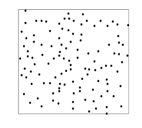
(a) Houston data set

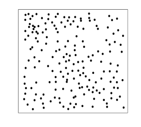
(b) LA data set

Figure 1: Real macro BS deployments.

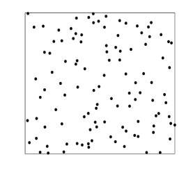
(a) Gauss DPP

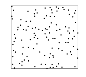
(b) Cauchy DPP

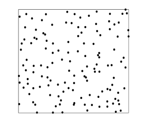
(c) Generalized Gamma DPP

Figure 2: DPP models fitted to the Houston BS deployment.

Based on the maximum likelihood (ML) estimate method which is implemented in the software package provided in [21], we have summarized the estimated parameters for different DPPs fitted to the Houston and LA data set in Table II and Table II. Realizations of the Gauss DPP, Cauchy DPP and Generalized Gamma DPP fitted to the Houston urban area deployment are shown in Fig. 2. From these figures, it can be qualitatively observed that the fitted DPPs are regularly distributed and close to the real BS deployments. In Section V, we will rigorously validate the accuracy of these DPP models based on different summary statistics.

TABLE I: DPP Parameters for the Houston Data Set

Model	$\lambda$	$\alpha$	$\nu$
Gauss DPP	0.4492	0.8417	$-$
Cauchy DPP	0.4492	1.558	3.424
Generalized Gamma DPP	0.4492	2.539	2.63

TABLE II: DPP Parameters for the LA Data Set

Model	$\lambda$	$\alpha$	$\nu$
Gauss DPP	0.2347	1.165	$-$
Cauchy DPP	0.2347	2.13	3.344
Generalized Gamma DPP	0.2347	3.446	2.505

III Analyzing Cellular Networks using Determinantal Point Processes

In this section, based on the three important computational properties discussed in Section II-B, we analyze several fundamental metrics for the analysis of downlink cellular networks with DPP configured BSs: (1) the empty space function; (2) the nearest neighbor function; (3) the mean interference and (4) the downlink SIR distribution.

III-A Empty Space Function

The empty space function is the cumulative distribution function (CDF) of the distance from the origin to its nearest point in the point process. It is also referred to as the spherical contact distribution. Consider $\Phi\sim\text{DPP}(K)$ and let $d(o,\Phi)=\inf\{\|x\|:x\in\Phi\}$; then the empty space function $F(r)$ is defined as: $F(r)=\mathbb{P}\left(d(o,\Phi)\leq r\right)$ for $r\geq 0$ [29].

In cellular networks, when each user is associated with its nearest BS, the empty space function provides the distribution of the distance from the typical user to its serving BS, which further dictates the statistics of the received signal power at the typical user.

Lemma 5

For any $\Phi\sim\text{DPP}(K)$, the empty space function $F(r)$ for $r\geq 0$ is given by:

$$F(r)=\sum_{n=1}^{+\infty}\frac{(-1)^{n-1}}{n!}\int_{\left(B(0,r)\right)^{n}}\det\left(K(x_{i},x_{j})\right)_{1\leq i,j\leq n}{\rm d}x_{1}...{\rm d}x_{n}.$$ (13)

Proof:

Choose $f(x)=-\log\mathbbm{1}_{\{\|x\|>r\}}$ for $x\in\mathbb{R}^{2}$, we have:

$$\mathbb{E}\left[\exp\left(-\int f(x)\Phi({\rm d}x)\right)\right] =\mathbb{E}\left[\exp\left(-\sum_{x_{i}\in\Phi}-\log\mathbbm{1}_{\|x_{i}\|>r}\right)\right]$$

$$=\mathbb{P}\left[d(o,\Phi)>r\right].$$

Therefore, based on Lemma 2, the empty space function is given by:

$$\allowdisplaybreaks F(r) =1-\mathbb{E}\left[\exp\left(-\int f(x)\Phi({\rm d}x)\right)\right]$$

$$=1-\sum_{n=0}^{+\infty}\frac{(-1)^{n}}{n!}\int_{(\mathbb{R}^{2})^{n}}\det\left(K(x_{i},x_{j})\right)_{1\leq i,j\leq n}\prod_{i=1}^{n}\left(1-\exp(\log\mathbbm{1}_{\{\|x_{i}\|>r\}})\right){\rm d}x_{1}...{\rm d}x_{n}$$

$$=\sum_{n=1}^{+\infty}\frac{(-1)^{n-1}}{n!}\int_{\left(B(0,r)\right)^{n}}\det\left(K(x_{i},x_{j})\right)_{1\leq i,j\leq n}{\rm d}x_{1}...{\rm d}x_{n}.$$

∎

Based on Lemma 5, we can also characterize the probability density function (PDF) $f(r)$ of the distance from the origin to its nearest point for all stationary and isotropic DPPs $\Phi$.

Corollary 2

Let $F(r)$ denote the empty space function for a stationary and isotropic DPP $\Phi$ with covariance function $K$. Then $f(r)\triangleq\frac{{\rm d}F(r)}{{\rm d}r}$ is given by:

$$f(r)=2\pi r\sum\limits_{n=0}^{+\infty}\frac{(-1)^{n}}{n!}\int_{(B(0,r))^{n}}\det(K(x_{i},x_{j}))_{0\leq i,j\leq n}\bigg{|}_{x_{0}=(r,0)}{\rm d}x_{1}...{\rm d}x_{n}.$$ (14)

Proof:

The proof is provided in Appendix C. ∎

III-B Nearest Neighbor Function

The nearest neighbor function gives the distribution of the distance from the typical point of a point process to its nearest neighbor in the same point process. For all stationary DPPs $\Phi$, the nearest neighbor function can be defined based on the reduced Palm distribution of $\Phi$ as: $D(r)=\mathbb{P}_{o}^{!}(d(o,\Phi)\leq r)$ [29].

In cellular networks, the nearest neighbor function provides the distribution of the distance from a typical BS to its nearest neighboring BS, which can be used as a metric to indicate the clustering/repulsive behavior of the network. Specifically, compared to the PPP, a regularly deployed network corresponds to a larger nearest neighbor function, while a clustered network corresponds to a smaller nearest neighbor function. Therefore, when each user is associated with its nearest BS, the dominant interferers in regularly deployed networks are farther from the serving BS than a completely random network.

Lemma 6

For any $\Phi\sim\text{DPP}(K)$ defined on $\mathbb{R}^{2}$, its nearest neighbor function $D(r)$ is given by:

$$D(r)=\sum_{n=1}^{+\infty}\frac{(-1)^{n-1}}{n!}\int_{\left(B(0,r)\right)^{n}}\det\left(K_{o}^{!}(x_{i},x_{j})\right)_{1\leq i,j\leq n}{\rm d}x_{1}...{\rm d}x_{n},$$ (15)

where $K_{o}^{!}(x,y)$ is:

$$K_{o}^{!}(x,y)=\frac{1}{K(0,0)}\det\left(\begin{array}[]{cc}K(x,y)&K(x,0)\\ K(0,y)&K(0,0)\end{array}\right).$$ (16)

Proof:

Denote $\tilde{\Phi}\sim\text{DPP}(K_{o}^{!}(x,y))$; then it follows from Lemma 4 that:

$$\mathbb{P}_{o}^{!}(d(o,\Phi)\leq r)=\mathbb{P}(d(o,\tilde{\Phi})\leq r).$$

Therefore, the proof can be concluded by applying Lemma 5 to the DPP $\tilde{\Phi}$. ∎

III-C Interference Distribution

In this section, we analyze properties of shot noise fields associated with a DPP. Our aim is to evaluate interference in cellular networks under two BS association schemes. Firstly, the BS to which the typical user is associated is assumed to be at an arbitrary but fixed location. We show that in this case, the mean interference is easy to characterize with DPP configured BSs. Secondly, each user is assumed to be associated with its nearest BS. In this case, we derive the Laplace transform of interference.

Throughout this part, the cellular BSs are assumed to be distributed according to a stationary and isotropic DPP $\Phi\sim\text{DPP}(K)$, while the mobile users are uniformly distributed and independent of the BSs. Since $\Phi$ is invariant under translations, we focus on the performance of the typical user which can be assumed to be located at the origin. The location for the serving BS of the typical user is denoted by $x_{0}$. Each BS $x\in\Phi$ has single transmit antenna with transmit power $P$, and it is associated with an independent mark $h_{x}$ which represents the small scale fading effects between the BS and the typical user. Independent Rayleigh fading channels with unit mean are assumed, which means $h_{x}\sim\exp(1)$ for $\forall x\in\Phi$. The shadowing effects are neglected, and the thermal noise power is assumed to be 0, i.e., negligible compared to interference power. In addition, the path loss function is denoted by $\mathit{l}(x):\mathbb{R}^{2}\mapsto\mathbb{R}^{+}$, which is a non-increasing function with respect to (w.r.t.) the norm of $x$.

III-C1 Interference with fixed associated BS scheme

Since $\Phi$ is invariant under translation and rotation, we assume the typical user located at the origin is served by the base station at $x_{0}=(r_{0},0)$, where $r_{0}$ denotes the distance from the origin to $x_{0}$. Conditionally on $x_{0}\in\Phi$ being the serving BS, the interference at the origin is: $I=\sum_{x_{i}\in\Phi\backslash x_{0}}Ph_{x_{i}}\mathit{l}(x_{i})$.

Lemma 7

Given $x_{0}=(r_{0},0)$ is the serving BS for the typical user located at the origin, the mean interference seen by this typical user is:

$$\mathbb{E}[I|x_{0}=(r_{0},0)]=P\int_{\mathbb{R}^{2}}K_{x_{0}}^{!}(x,x)\mathit{l}(x){\rm d}x,$$ (17)

where $K_{x_{0}}^{!}(\cdot,\cdot)$ is given in (8).

Proof:

From Lemma 4, the mean interference can be expressed as:

$$\mathbb{E}[\sum_{x_{i}\in\Phi\backslash x_{0}}Ph_{x_{i}}\mathit{l}(x_{i})|x_{0}=(r_{0},0)]= \mathbb{E}[\sum_{x_{i}\in\tilde{\Phi}}Ph_{x_{i}}\mathit{l}(x_{i})]$$

$$\overset{(a)}{=} P\int_{\mathbb{R}^{2}}\int_{\mathbb{R}^{+}}h\mathit{l}(x)K_{x_{0}}^{!}(x,x)\exp(-h){\rm d}h{\rm d}x$$

$$= P\int_{\mathbb{R}^{2}}K_{x_{0}}^{!}(x,x)\mathit{l}(x){\rm d}x,$$

where $\tilde{\Phi}\sim\text{DPP}(K_{x_{0}}^{!})$ follows from Lemma 4, and (a) follows from Campbell’s theorem. ∎

In fact, all the higher order moment measures of the interference can be calculated similarly based on Definition 1 and Lemma 4.

III-C2 Interference with nearest BS association scheme

In this part, we consider the BS association scheme where each user is served by its nearest BS. In single tier cellular networks, the nearest BS association scheme provides the highest average received power for each user.

For a user located at $y\in\mathbb{R}^{2}$, its associated BS is denoted by $x^{*}(y)=\underset{x\in\Phi}{\operatorname{argmin}}\|x-y\|$. Consider the typical user located at the origin and its associated BS $x^{*}(0)$. The interference at the typical user is then given by $I=\sum\limits_{x_{i}\in\Phi\backslash x^{*}(0)}Ph_{x_{i}}\mathit{l}(x_{i})$, where $h_{x_{i}}\sim\exp(1)$ denotes the Rayleigh fading variable from $x_{i}$ to the origin. In the next theorem, we provide the general result which characterizes the Laplace transform of interference conditional on the position of the BS nearest to the typical user.

Theorem 1

Conditionally on $x^{*}(0)=x_{0}$ being the serving BS of the typical user at the origin, if $f(x,h_{x})=sPh_{x}\mathit{l}(x)\mathbbm{1}_{|x|\geq r_{0}}-\log\mathbbm{1}_{|x|\geq r_{0}}$ satisfies the conditions in Lemma 3, then the Laplace transform of the interference at the typical user is:

$$\small\mathbb{E}[e^{-sI}|x^{*}(0)=x_{0}]=\frac{\sum\limits_{n=0}^{+\infty}\frac{(-1)^{n}}{n!}\int_{(\mathbb{R}^{2})^{n}}\det(K_{x_{0}}^{!}(x_{i},x_{j}))_{1\leq i,j\leq n}\prod\limits_{i=1}^{n}[1-\frac{\mathbbm{1}_{|x_{i}|\geq r_{0}}}{1+sP\mathit{l}(x_{i})}]{\rm d}x_{1}...{\rm d}x_{n}}{\sum\limits_{n=0}^{+\infty}\frac{(-1)^{n}}{n!}\int_{B(0,r_{0})^{n}}\det(K_{x_{0}}^{!}(x_{i},x_{j}))_{1\leq i,j\leq n}{\rm d}x_{1}...{\rm d}x_{n}},$$ (18)

where $r_{0}=|x^{*}(0)|$ and $K_{x_{0}}^{!}(\cdot,\cdot)$ is given in (8).

Proof:

Denote $\tilde{\Phi}\sim\text{DPP}(K_{x_{0}}^{!})$, we have:

$$\mathbb{E}[\exp(-sI)|x^{*}(0)=x_{0}]= \mathbb{E}[\exp(-sI)|x_{0}\in\Phi,\Phi(B^{o}(0,r_{0}))=0]$$

$$\overset{(a)}{=} \mathbb{E}_{x_{0}}^{!}[\exp(-s\sum_{x_{i}\in\Phi\cap B^{c}(0,r_{0})}Ph_{x_{i}}\mathit{l}(x_{i}))|\Phi(B^{o}(0,r_{0}))=0]$$

$$\overset{(b)}{=} \mathbb{E}[\exp(-s\sum_{x_{i}\in\tilde{\Phi}\cap B^{c}(0,r_{0})}Ph_{x_{i}}\mathit{l}(x_{i}))\mathbbm{1}_{\tilde{\Phi}(B^{o}(0,r_{0}))=0}]/\mathbb{P}[\tilde{\Phi}(B^{o}(0,r_{0}))=0]~{},$$ (19)

where (a) follows from the Bayes’ rule, and the fact that conditionally on $x_{0}\in\Phi$, $(\Phi-\delta_{x_{0}})(B^{o}(0,r_{0}))=0$ is equivalent to $\Phi(B^{o}(0,r_{0}))=0$ since $x_{0}$ lies on the boundary of the open ball $B^{o}(0,r_{0})$. In addition, (b) follows from the fact that for all random variables $X$ and events $A$, $\mathbb{E}[X|A]=\frac{\mathbb{E}[X\mathbbm{1}_{A}]}{\mathbb{P}(A)}$.

Next, it is clear that the denominator in (19) is given by:

$$~{}\allowdisplaybreaks\mathbb{P}[\tilde{\Phi}(B^{o}(0,r_{0}))=0] =\sum\limits_{n=0}^{+\infty}\frac{(-1)^{n}}{n!}\int_{B(0,r_{0})^{n}}\det(K_{x_{0}}^{!}(x_{i},x_{j}))_{1\leq i,j\leq n}{\rm d}x_{1}...{\rm d}x_{n}.$$ (20)

The numerator in (19) is calculated as:

$$\mathbb{E}[\exp(-s\sum_{x_{i}\in\tilde{\Phi}\cap B^{c}(0,r_{0})}Ph_{x_{i}}\mathit{l}(x_{i}))\mathbbm{1}_{\tilde{\Phi}(B^{o}(0,r_{0}))=0}]$$

$$\overset{(a)}{=} \sum\limits_{n=0}^{+\infty}\frac{(-1)^{n}}{n!}\int_{(\mathbb{R}^{2})^{n}}\int_{(\mathbb{R}^{+})^{n}}\det(K_{x_{0}}^{!}(x_{i},x_{j}))_{1\leq i,j\leq n}\prod\limits_{i=1}^{n}[(1-$$

$$\exp(-sPh_{x_{i}}\mathit{l}(x_{i})\mathbbm{1}_{|x_{i}|\geq r_{0}}+\log\mathbbm{1}_{|x_{i}|\geq r_{0}}))\exp(-h_{x_{i}}){\rm d}h_{i}]{\rm d}x_{1}...{\rm d}x_{n}$$

$$= \sum\limits_{n=0}^{+\infty}\frac{(-1)^{n}}{n!}\int_{(\mathbb{R}^{2})^{n}}\det(K_{x_{0}}^{!}(x_{i},x_{j}))_{1\leq i,j\leq n}\prod\limits_{i=1}^{n}[1-\frac{\mathbbm{1}_{|x_{i}|\geq r_{0}}}{1+sP\mathit{l}(x_{i})}]{\rm d}x_{1}...{\rm d}x_{n},~{}$$ (21)

where (a) is obtained from Lemma 3. Finally, substituting (20) and (21) into (19) yields the result. ∎

Remark 2

In contrast with what happens in the PPP case, because of the repulsion among DPP points, $\Phi\cap B^{c}(0,r_{0})$ and $\Phi\cap B^{o}(0,r_{0})$ are not independent.

Remark 3

If $\Phi$ is a stationary PPP with intensity $\lambda$, then by substituting $\det(K(x_{i},x_{j}))_{1\leq i,j\leq n}=\det(K_{x_{0}}^{!}(x_{i},x_{j}))_{1\leq i,j\leq n}=\lambda^{n}$, Theorem 1 gives the Laplace transform of the interference at the typical user to be:

$$\mathbb{E}[e^{-sI}|x^{*}(0)=x_{0}]=\exp\left(-\lambda\int_{B^{c}(0,r_{0})}(1-\frac{1}{1+sP\mathit{l}(x)}){\rm d}s\right),$$

which is consistent with (12) in [2].

Since the Laplace transform fully characterizes the probability distribution, many important performance metrics can be derived using Theorem 1. Specifically, the next lemma gives the mean interference under the nearest BS association scheme.

Lemma 8

The mean interference at the typical user conditional on $x^{*}(0)=x_{0}$ is:

$$~{}\mathbb{E}[I|x^{*}(0)=x_{0}]=\frac{\sum\limits_{n=0}^{+\infty}\frac{(-1)^{n}}{n!}\int_{(B(0,r_{0}))^{n}}\int_{B^{c}(0,r_{0})}\det(K_{x_{0}}^{!}(x_{i},x_{j}))_{1\leq i,j\leq n+1}P\mathit{l}(x_{1}){\rm d}x_{1}...{\rm d}x_{n+1}}{\sum\limits_{n=0}^{+\infty}\frac{(-1)^{n}}{n!}\int_{B(0,r_{0})^{n}}\det(K_{x_{0}}^{!}(x_{i},x_{j}))_{1\leq i,j\leq n}{\rm d}x_{1}...{\rm d}x_{n}},$$ (22)

where $r_{0}=|x_{0}|$.

Proof:

The proof is provided in Appendix D. ∎

Since the DPPs are assumed to be stationary and isotropic, thus only the distance from the origin to its nearest BS will affect the mean interference result, which can be observed from Lemma 8.

III-D SIR Distribution

Based on the same assumptions as in Section III-C, we derive the SIR distribution as the complementary cumulative distribution function (CCDF) of the SIR at the typical user under the nearest BS association scheme. Denote by $x^{*}(0)$ the BS to which the typical user at the origin associates, its received SIR can be expressed as:

$$~{}\text{SIR}(0,\Phi)=\frac{Ph_{x_{0}}\mathit{l}(x^{*}(0))}{\sum_{x_{i}\in\Phi\setminus x^{*}(0)}Ph_{x_{i}}\mathit{l}(x_{i})}.$$ (23)

Lemma 9

The SIR distribution for the typical user at the origin, given $x^{*}(0)=x_{0}$ is:

$$\mathbb{P}[\text{SIR}(0,\Phi)>T|x^{*}(0)=x_{0}]$$

$$= \frac{\sum\limits_{n=0}^{+\infty}\frac{(-1)^{n}}{n!}\int_{(\mathbb{R}^{2})^{n}}\det(K_{x_{0}}^{!}(x_{i},x_{j}))_{1\leq i,j\leq n}\prod\limits_{i=1}^{n}[1-\frac{\mathbbm{1}_{|x_{i}|\geq r_{0}}}{1+T\mathit{l}(x_{i})/\mathit{l}(x_{0})}]{\rm d}x_{1}...{\rm d}x_{n}}{\sum\limits_{n=0}^{+\infty}\frac{(-1)^{n}}{n!}\int_{B(0,r_{0})^{n}}\det(K_{x_{0}}^{!}(x_{i},x_{j}))_{1\leq i,j\leq n}{\rm d}x_{1}...{\rm d}x_{n}}~{},$$ (24)

where $r_{0}=|x_{0}|$.

Proof:

Since the channels are subject to Rayleigh fading with unit mean, we have:

$$\mathbb{P}[\text{SIR}(0,\Phi)>T|x^{*}(0)=x_{0}]= \mathbb{P}[\frac{h_{0}\mathit{l}(x_{0})}{I}>T|x^{*}(0)=x_{0}]$$

$$= \mathbb{E}[\exp(-\frac{T}{\mathit{l}(x_{0})}I)|x^{*}(0)=x_{0}],$$

and the result follows from Theorem 1. ∎

In Corollary 2, the probability density function for the distance from the origin to its nearest BS has been characterized. Therefore, by combining Corollary 2 and Lemma 9, we are able to compute the SIR distribution of the typical user under the nearest BS association scheme.

Theorem 2

The SIR distribution of the typical user at the origin is given by:

$$\small\begin{split}&\mathbb{P}(\text{SIR}(0,\Phi)>T)\\ &=\int_{0}^{+\infty}\lambda 2\pi\left[\sum\limits_{n=0}^{+\infty}\frac{(-1)^{n}}{n!}\int_{(\mathbb{R}^{2})^{n}}\det(K_{x_{0}}^{!}(x_{i},x_{j}))_{1\leq i,j\leq n}\prod\limits_{i=1}^{n}[1-\frac{\mathbbm{1}_{|x_{i}|\geq r_{0}}}{1+T\mathit{l}(x_{i})/\mathit{l}(x_{0})}]\bigg{|}_{x_{0}=(r_{0},0)}{\rm d}x_{1}...{\rm d}x_{n}\right]r_{0}{\rm d}r_{0}.\end{split}$$ (25)

Proof:

When expressing the location of the closest BS to the typical user in polar form as $x^{*}(0)=(r_{0},\theta)$, we know that $x^{*}(0)$ admits the probability density $\frac{{\rm d}\theta}{2\pi}f(r_{0}){\rm d}r_{0}$, where $f(r_{0})$ is given in Corollary 2. Therefore, we have:

$$\mathbb{P}(\text{SIR}(0,\Phi)>T) =\int_{0}^{+\infty}\int_{0}^{2\pi}\mathbb{P}[\text{SIR}(0,\Phi)>T|x^{*}(0)=(r_{0},\theta)]\frac{1}{2\pi}f(r_{0}){\rm d}\theta{\rm d}r_{0}$$

$$\overset{(a)}{=}\int_{0}^{+\infty}\mathbb{P}[\text{SIR}(0,\Phi)>T|x^{*}(0)=(r_{0},0)]f(r_{0}){\rm d}r_{0},$$

where (a) is because the DPP is stationary and isotropic, so that the angle of $x_{0}$ will not affect the result of $\mathbb{P}[\text{SIR}(0,\Phi)>T|x^{*}(0)=(r_{0},\theta)]$. It follows from (9) that $\det(K_{x_{0}}^{!}(x_{i},x_{j}))_{1\leq i,j\leq n}=\frac{1}{K(x_{0},x_{0})}\det(K(x_{i},x_{j}))_{0\leq i,j\leq n}$, then the proof is completed by applying Corollary 2 and Lemma 9. ∎

Remark 4

If we choose $\Phi$ as a stationary PPP with intensity $\lambda$, i.e., $\det(K(x_{i},x_{j}))_{1\leq i,j\leq n}=\det(K_{x_{0}}^{!}(x_{i},x_{j}))_{1\leq i,j\leq n}=\lambda^{n}$, then Theorem 2 leads to the same result as [2, Theorem 2].

IV Numerical Evaluation using Quasi-Monte Carlo Integration Method

In this section, we provide the numerical method used to evaluate the analytical results derived in Section III. The Laplace functional of DPPs involves a series representation, where each term is a multi-dimensional integration. Therefore, we adopt the Quasi-Monte Carlo (QMC) integration method [30] for efficient numerical integration.

The QMC integration method approximates the multi-dimensional integration of function $f:[0,1]^{n}\rightarrow\mathbb{R}$ as:

$$\int_{[0,1]^{n}}f(\textbf{x})d\textbf{x}\approx\frac{1}{N}\sum_{n=0}^{N-1}f(\textbf{x}_{n}).$$

The sample points $\textbf{x}_{0},...,\textbf{x}_{N-1}\in[0,1]^{n}$ are chosen deterministically in the QMC method, and we use the Sobol points generated in MATLAB as the choice for sample points [31]. Compared to the regular Monte Carlo integration method which uses a pseudo-random sequence as the sample points, the QMC integration method converges much faster.

In the following, we will focus on the numerical results using the Gauss DPP fitted to the Houston and LA data set. The modeling accuracy of the fitted Gauss DPPs compared to the real data sets will be validated in Section V. In addition, our simulation results for each metric are based on the average of 1000 realizations of the fitted Gauss DPP.

IV-A Empty Space Function

Since the QMC integration method requires integration over the unit square, (13) can be rewritten as:

$$~{}\small F(r)=\sum_{n=1}^{+\infty}\frac{(-1)^{n-1}(2r)^{2n}}{n!}\int_{\left([0,1]\times[0,1]\right)^{n}}\det\left(K_{0}(2r(x_{i}-x_{j}))\right)_{1\leq i,j\leq n}\prod_{i}\mathbbm{1}_{\{\|x_{i}-(\frac{1}{2},\frac{1}{2})\|\leq\frac{1}{2}\}}{\rm d}x_{1}...{\rm d}x_{n},$$ (26)

where $K_{0}(x)$ is the covariance function for the DPP $\Phi$.

The accuracy of (26) is verified by computing the empty space function of the Gauss DPP fitted to the Houston and LA data set respectively. Specifically, for the Gauss DPP model, $K_{0}(x)=\lambda\exp(-\|x/\alpha\|^{2})$, where $\lambda$ and $\alpha$ are chosen according to Table II and Table II. Fig. 3 shows the QMC integration results of (26) with different numbers of Sobol points, as well as the simulation result for the fitted Gauss DPP. We have observed that when the number of Sobol points is $2^{11}$, (26) can be computed very efficiently (in a few seconds) and the QMC integration results are accurate except for the part where $F(r)$ is over 95%. In contrast, if the number of Sobol points is increased to $2^{15}$, the QMC integration method is almost 10 times slower while the results are accurate for a much larger range of $r$.

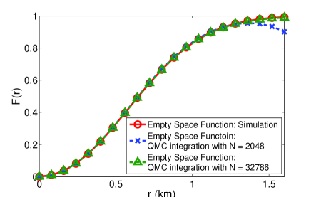
(a) Houston data set

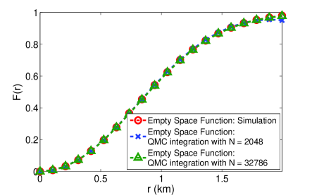
(b) LA data set

Figure 3: Empty space function of the fitted Gauss DPP.

IV-B Nearest Neighbor Function

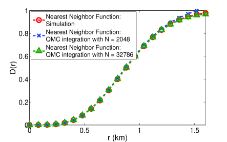
(a) Houston data set

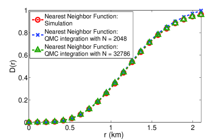
(b) LA data set

Figure 4: Nearest neighbor function of the fitted Gauss DPP.

The QMC integration method is also efficient in the numerical evaluation of the nearest neighbor function. Similar to the empty space function, the QMC integration method with $N=2^{11}$ takes a few seconds to return $D(r)$ in Fig. 4, which is accurate up to 95%. By contrast, the QMC integration method is more accurate but almost ten times slower when the number of sample points is increased to $N=2^{15}$.

IV-C Mean Interference

In this part, the mean interference of the Gauss DPP is numerically evaluated for the two BS association schemes discussed in Section III-C. The path loss model is chosen as $\mathit{l}(x)=\min(1,|x|^{-\beta})$, where $\beta>2$ is the path loss exponent.

IV-C1 Mean interference with fixed associated BS scheme

Corollary 3

Conditionally on $x_{0}=(r_{0},0)$ as the serving BS for the typical user, the mean interference at the typical user when BSs are distributed according to the Gauss DPP with parameters $(\lambda,\alpha)$ is given by:

$$\mathbb{E}[I|x_{0}=(r_{0},0)]=\frac{P\pi\lambda\beta}{\beta-2}-2P\pi\lambda\exp(-\frac{2r_{0}^{2}}{\alpha^{2}})(A_{1}(r_{0})+A_{2}(r_{0})),$$

where $A_{1}(r_{0})=\int_{0}^{1}\exp(-\frac{2r^{2}}{\alpha^{2}})I_{0}(\frac{4rr_{0}}{\alpha^{2}})r{\rm d}r$, and $A_{2}(r_{0})=\int_{1}^{\infty}\exp(-\frac{2r^{2}}{\alpha^{2}})r^{1-\beta}I_{0}(\frac{4rr_{0}}{\alpha^{2}}){\rm d}r$. Here $I_{0}(\cdot)$ denotes the modified Bessel function of first kind with parameter $\nu=0$ [32].

Proof:

Based on the fact that $\int_{0}^{2\pi}\exp(\pm\beta\cos(x)){\rm d}x=2\pi I_{0}(\beta)$ [32, p. 491], this corollary can be derived by substituting the Gauss DPP kernel into Lemma 7. ∎

In Fig. 5, the mean interference for the Gauss DPP fitted to the Houston and LA data sets are provided under different path loss exponents with $P=1$. From Fig. 5, it can be observed that the mean interference increases as $r_{0}$ increases; this is because it increases the probability for the existence of a strong interferer close to the typical user. In addition, given $r_{0}$, the mean interference is decreasing when the path loss exponent $\beta$ increases; this is because the path loss function is decreasing with respect to $\beta$ for all interferers.

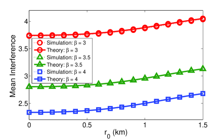
(a) Houston data set

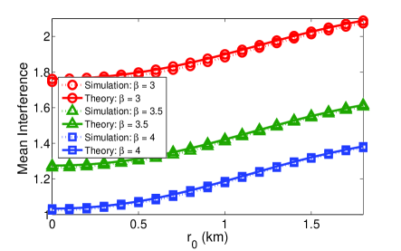
(b) LA data set

Figure 5: Mean interference under the fixed associated BS scheme.

IV-C2 Mean interference with nearest BS association scheme

The Quasi-Monte Carlo integration method is adopted to evaluate the mean interference under the nearest BS association scheme, which is given in (22). In Fig. 6, the mean interference is evaluated when the path loss exponent $\beta$ is 3, 3.5, 4. It can be observed from Fig. 6 that when $r_{0}$ (i.e., the distance from the typical user to its nearest BS) increases, the mean interference decreases. This is because the strong interferers are farther away from the typical user when $r_{0}$ increases, which leads to a smaller aggregate interference. This is quite different from the case when the BS associated to the typical user is assumed to be at some fixed location. In addition, since the path loss function $\mathit{l}(x)$ is non-increasing with respect to $\beta$ given the norm of $x$, the mean interference decreases when $\beta$ increases for a given $r_{0}$.

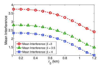
(a) Houston data set

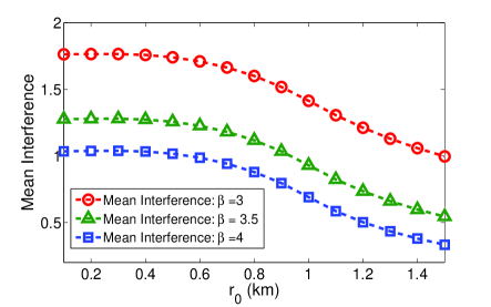
(b) LA data set

Figure 6: Mean interference under the nearest BS association scheme.

IV-D SIR Distribution

The QMC integration method can, in principle, be used to numerically evaluate (25). However, it is time consuming due to the need to evaluate multiple integrations over $\mathbb{R}^{2}$. Therefore, we use the diagonal approximation of the matrix determinant [33] to roughly estimate (25). Specifically, the determinant of matrix $\left(K(x_{i},x_{j})\right)_{1\leq i,j\leq n}$ is approximated as $\det(\left(K(x_{i},x_{j})\right)_{1\leq i,j\leq n})\approx\prod_{i=1}^{n}K(x_{i},x_{i})$ under the diagonal approximation.

Lemma 10

Under the diagonal approximation, the SIR distribution for the typical user is approximated as:

$$\mathbb{P}(\text{SIR}(0,\Phi)>T)\approx\int_{0}^{+\infty}\lambda 2\pi r_{0}\exp\left(-\int_{\mathbb{R}^{2}}K_{x_{0}}^{!}(x,x)(1-\frac{\mathbbm{1}_{|x|\geq r_{0}}}{1+T\mathit{l}(x)/\mathit{l}(x_{0})})\bigg{|}_{x_{0}=(r_{0},0)}{\rm d}x\right){\rm d}r_{0}.$$ (27)

Lemma 10 can be proved by applying diagonal approximation to Theorem 2, thus we omit the proof.

Next, we evaluate the accuracy of Lemma 10 by assuming the BSs are distributed according to the Gauss DPP. In addition, the power-law path loss model with path loss exponent $\beta>2$ is used for simplicity, i.e., $\mathit{l}(x)=\|x\|^{-\beta}$ for $x\in\mathbb{R}^{2}$.

Corollary 4

When BSs are distributed according to the Gauss DPP with parameters $(\lambda,\alpha)$, the SIR distribution can be approximated under the diagonal approximation as:

$$\allowdisplaybreaks\mathbb{P}(\text{SIR}(0,\Phi)>T)\approx \int_{0}^{+\infty}\lambda 2\pi r_{0}\exp\biggl{(}-\lambda 2\pi\biggl{[}\int_{0}^{r0}(1-\exp(-\frac{2(r^{2}+r_{0}^{2})}{\alpha^{2}})I_{0}(\frac{4rr_{0}}{\alpha^{2}}))r{\rm d}r$$

$$+\int_{r_{0}}^{+\infty}(1-\exp(-\frac{2(r^{2}+r_{0}^{2})}{\alpha^{2}})I_{0}(\frac{4rr_{0}}{\alpha^{2}}))\frac{Tr_{0}^{\beta}r}{Tr_{0}^{\beta}+r^{\beta}}{\rm d}r\biggl{]}\biggl{)}{\rm d}r_{0},$$ (28)

where $I_{0}(\cdot)$ denotes the modified Bessel function of first kind with parameter $\nu=0$.

Proof:

Based on the fact that $\int_{0}^{2\pi}\exp(\pm\beta\cos(x)){\rm d}x=2\pi I_{0}(\beta)$ [32, p. 491], this corollary can be derived by substituting the Gauss DPP kernel into Lemma 10. ∎

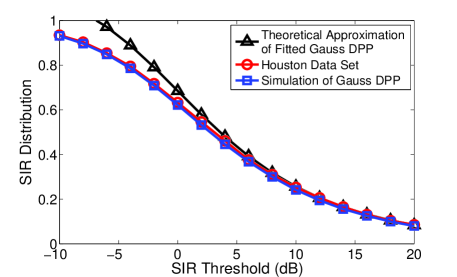
(a) Houston data set

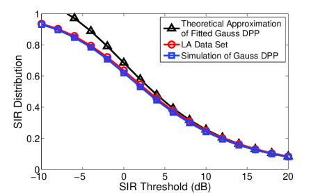
(b) LA data set

Figure 7: Diagonal approximation to the SIR distribution of the fitted Gauss DPP.

The QMC integration method is used to evaluate (28) with path loss exponent $\beta=4$, and the result for the Gauss DPP fitted to Houston data set is plotted in Fig. 7. It can be observed that the diagonal approximation to the coverage probability is accurate compared to the simulation result in the high SIR regime, i.e., when the SIR threshold is larger than 6 dB. The same trend can also be found for the LA data set. Therefore, we can use the diagonal approximation as an accurate estimate for the coverage probability in the high SIR regime.

V Goodness-of-fit for Stationary DPPs to Model BS Deployments

Given that the stationary DPP models are tractable, we provide rigorous investigation of their modeling accuracy to real BS deployments in this section. Our simulations are based on the publicly available package for DPP models [21] implemented in R, which is used as a supplement to the Spatstat library [34].

V-A Summary Statistics

To test the goodness-of-fit of these DPP models, we have used Ripley’s K function and the coverage probability as performance metrics, which are described below:

Ripley’s K function: Ripley’s K function is a second order spatial summary statistic defined for stationary point processes. It counts the mean number of points within distance $r$ of a given point in the point process excluding the point itself. Formally, the K function $\mathbb{K}(r)$ for a stationary and isotropic point process $\Phi$ with intensity $\lambda$ is defined as:

$$\allowdisplaybreaks\mathbb{K}(r)=\frac{\mathbb{E}_{o}^{!}\left(\Phi(B(0,r))\right)}{\lambda},$$ (29)

where $\mathbb{E}_{o}^{!}(\cdot)$ is the expectation with respect to the reduced Palm distribution of $\Phi$.

The K-function is used as a measure of repulsiveness/clustering of spatial point processes. Specifically, compared to the PPP which is completely random, a repulsive point process model will have a smaller K function, while a clustered point process model will have a larger K function.

Coverage Probability: The coverage probability is defined as the probability that the received SINR at the typical user is larger than the threshold $T$. When measuring the fitting accuracy of spatial point processes to real BS deployments, metrics related to the wireless system such as the coverage probability are more practical. In particular, the coverage probability also depends on the repulsive/clustering behavior of the underlying point process used to model the BS deployment. Compared to the fitted PPP, due a larger empty space function, the distance from the typical user to its serving BS is stochastically less in a fitted repulsive point process. Similarly, due to a smaller nearest neighbor function, the fitted repulsive point process has stochastically larger distance from the serving BS to its closest interfering BS than the PPP case. Therefore, from (23), a larger coverage probability is expected when the BS deployments are modeled by more repulsive spatial point processes. We will use the same parameter assumptions as in Section IV-D for evaluating the coverage probability. Since the thermal noise power is assumed to be 0, the CCDF of SIR at the typical user, i.e., $\mathbb{P}(\text{SIR}(0,\Phi)>T)$, coincides with its coverage probability with threshold $T$.

V-B Hypothesis Testing using Summary Statistics

In this part, we evaluate the goodness-of-fit of stationary DPP models using the summary statistics discussed above. Particularly, we fit the real BS deployments in Fig. 1 to the Gauss, Cauchy and Generalized Gamma DPPs.

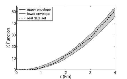
(a) Houston data set

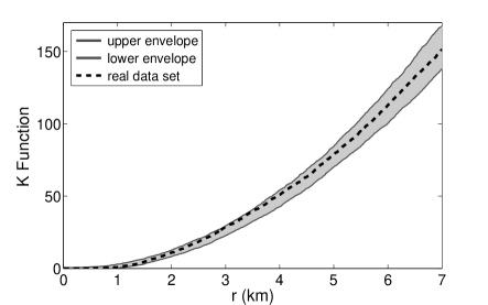
(b) LA data set

Figure 8: K function of the fitted Gauss DPP.

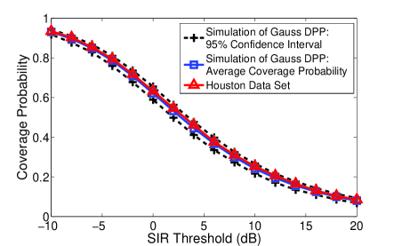
(a) Houston data set

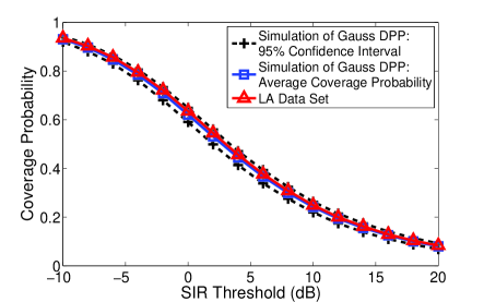
(b) LA data set

Figure 9: Coverage probability of the fitted Gauss DPP.

To evaluate the goodness-of-fit for these DPP models, we generate 1000 realizations of each DPP model and examine whether the simulated DPPs fit with the behavior of real BS deployments in terms of the summary statistics. Specifically, based on the null hypothesis that real BS deployments can be modeled as realizations of DPPs, we verify whether the K-function of the real data set lies within the envelope of the simulated DPPs. We use similar testing method for the coverage probability; a 95% confidence interval is used for evaluation.

Goodness-of-fit for Gauss DPP Model: The testing results for the K function of the fitted Gauss DPP are given in Fig. 8, which clearly show that the K functions of the real BS deployments lie within the envelope of the fitted Gauss DPP. The coverage probability for the fitted Gauss DPP is provided in Fig. 9, from which it can be observed that the coverage probabilities of the Houston and LA data sets lie within the 95% confidence interval of the simulated Gauss DPPs. In addition, the average coverage probability of the fitted Gauss DPP is slightly lower than that of real data sets, which means that the fitted Gauss DPP corresponds to a slightly smaller repulsiveness than the real deployments.

Therefore, in terms of the above summary statistics, the Gauss DPP model can be used as a reasonable point process model for real BS deployments. In addition, due to the concise definition of its kernel, the shot noise analysis of the Gauss DPP is possible, which further motivates the use of Gauss DPPs to model real-world macro BS deployments.

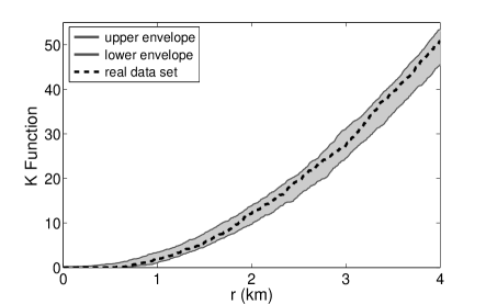
(a) K function

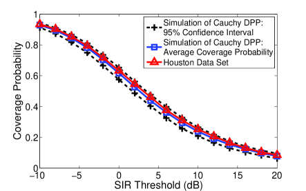
(b) Coverage probability

Figure 10: Goodness-of-fit for the Cauchy DPP fitted to the Houston data set.

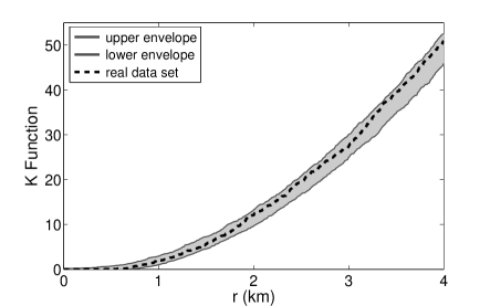
(a) K function

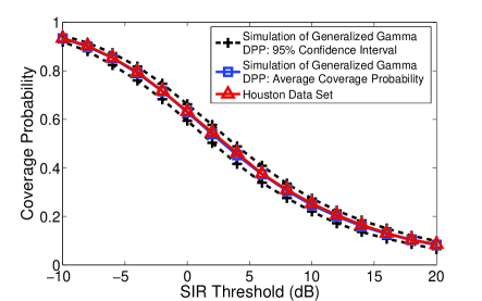
(b) Coverage probability

Figure 11: Goodness-of-fit for the Generalized Gamma DPP fitted to the Houston data set.

Goodness-of-fit for the Cauchy DPP Model: Based on the same method as for the Gauss DPP model, we tested the goodness-of-fit for the Cauchy DPP model. The fitting results for the Houston data set are shown in Fig. 10, from which it can be concluded that the Cauchy DPP model is also a reasonable point process model for real BS deployments. Similar fitting results are also observed for the LA data set, and thus we omit the details. Compared to the fitted Gauss DPP, the average coverage probability for the fitted Cauchy DPP in Fig. 10 is slightly lower than that in Fig. 9, which means the fitted Cauchy DPP corresponds to a smaller repulsiveness than the Gauss DPP.

Goodness-of-fit for the Generalized Gamma DPP Model: The goodness-of-fit for the Generalized Gamma DPP fitted to the Houston data set is evaluated in Fig. 11 (the LA data set has similar fitting results). The Generalized Gamma DPP provides the best fit among all these DPP models, especially in terms of coverage probability. In Fig. 11, the average coverage probability of the fitted Generalized Gamma DPP almost exactly matches the real BS deployment, while the average coverage probability of the fitted Gauss DPP and the fitted Cauchy DPP all stay below the real data set. This is because the Generalized Gamma DPP corresponds to a higher repulsiveness (which will be proved in Section V-C), from which a larger coverage probability is expected.

Goodness-of-fit for the PPP and the perturbed hexagonal model: Finally, the goodness-of-fit for the PPP and the perturbed hexagonal grid model are studied. The perturbed hexagonal grid model is obtained by independently perturbing each point of a hexagonal grid in the random direction by a distance $d$ [17]. This distance is uniformly distributed between 0 and $\eta r$, with $r$ being the radius of the hexagonal cells and $\eta$ is chosen as 0.5 in our simulation. Fig. 12 depicts the coverage probability of the PPP and of the perturbed hexagonal grid model, which correspond to a lower bound and an upper bound of the actual coverage probability respectively. This is because the PPP exhibits complete spatial randomness while the perturbed grid model maintains good spatial regularity.

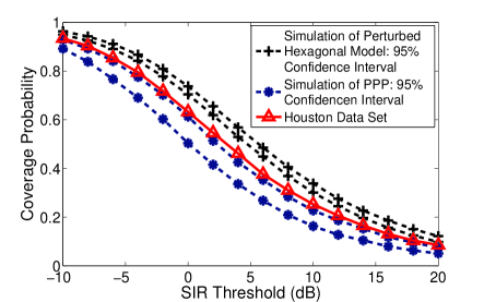
(a) Houton data set

(b) LA data set

Figure 12: Coverage probability of the PPP and the perturbed grid model.

V-C Repulsiveness of Different DPPs

In order to explain why the Generalized Gamma DPP has larger repulsiveness, we use the metric suggested in [21] to measure the repulsiveness of different DPPs. Specifically, from Lemma 4, the intensity measure of a stationary DPP $\Phi$ under its reduced Palm distribution is $\rho_{o}^{(1)}(x)=\rho^{(2)}(0,x)/\rho^{(1)}(x)$, where $\rho^{(2)}$ and $\rho^{(1)}$ are the second and the first order product density of $\Phi$. By calculating the difference of the total expected number of points under the probability distribution $\mathbb{P}$ and the reduced Palm distribution $\mathbb{P}_{o}^{!}$, the repulsiveness of a stationary DPP $\Phi$ with intensity $\lambda$ can be measured using the following metric [21]:

$$\small\mu=\int_{\mathbb{R}^{2}}\left[\lambda-\rho_{o}^{(1)}(x)\right]{\rm d}x=\frac{1}{\lambda}\int_{\mathbb{R}^{2}}|K_{0}(x)|^{2}{\rm d}x=\frac{1}{\lambda}\int_{\mathbb{R}^{2}}|\varphi(x)|^{2}{\rm d}x,$$ (30)

where $K_{0}(x)$ and $\varphi(x)$ denote the covariance function and spectral density of $\Phi$ respectively.

PPP has $\mu=0$ due to Slivnyak’s theorem, while the grid-based model has $\mu=1$ since the point at the origin is excluded under reduced Palm distribution. Generally, larger value of $\mu$ will correspond to a more repulsive point process. This repulsiveness measure for the Gauss, Cauchy and Generalized Gamma model can be calculated as: $\mu_{\text{gauss}}=\lambda\pi\alpha^{2}/2$, $\mu_{\text{cauchy}}=\lambda\pi\alpha^{2}/(2\nu+1)$, and $\mu_{\text{gengamma}}=\lambda\nu\alpha^{2}/(2^{1+2/\nu}\pi\Gamma(2/\nu))$. Based on the parameters in Table II, we can calculate the repulsiveness measure of each DPP model fitted to the Houston data set as $\mu_{\text{gauss}}=0.4999$, $\mu_{\text{cauchy}}=0.4365$ and $\mu_{\text{gengamma}}=0.5905$. Similarly, the repulsiveness measure of each DPP model fitted to the LA data set is given by $\mu_{\text{gauss}}=0.5004$, $\mu_{\text{cauchy}}=0.4351$, $\mu_{\text{gengamma}}=0.5479$. Therefore, it can be concluded that the fitted Generalized Gamma DPP has the largest repulsiveness, followed by the fitted Gauss DPP, while the fitted Cauchy DPP is the least repulsive. Since higher repulsiveness will result in more regularity for the point process, a Generalized Gamma DPP generally corresponds to a larger average coverage probability.

VI Performance Comparisons of DPPs and PPPs

Based on the analytical, numerical and statistical results from previous sections, we demonstrate that the DPPs are more accurate than the PPPs to predict key performance metrics in cellular networks for the following reasons.

Firstly, since the DPPs have more regularly spaced point pattern, they will have larger empty space function than the PPPs. Equivalently, this means the distance from the origin to its closest point on the DPPs fitted to real deployments is stochastically less than the PPPs, which can be observed in Fig. 13(a) for the Gauss DPP. Therefore, if each user is associated with its nearest BS, DPPs will lead to a stronger received power at the typical user compared to PPPs in the stochastic dominance sense.

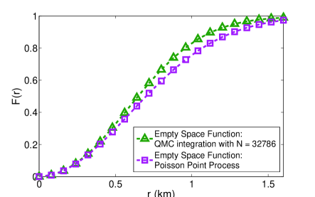
(a) Empty space function

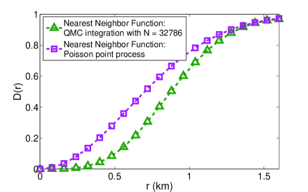
(b) Nearest neighbor function

Figure 13: Comparison of the Gauss DPP and PPP fitted to Houston data set.

Secondly, the fitted DPPs will have smaller nearest neighbor function than the PPP, which can be observed in Fig. 13(b) for the Gauss DPP. In addition, we can also observe from Fig. 13(b) that the nearest neighbor function for the Gauss DPP is much smaller than the PPP when $r$ is small. This indicates that the PPP will largely overestimate the nearest neighbor function when $r$ is small, which leads to much closer strong interfering BSs compared to the Gauss DPP.

In addition to the empty space function and the nearest neighbor function, the DPPs are also more accurate in estimating the interference and coverage probability than the PPP. When each user is associated with an arbitrary but fixed BS, an immediate implication of Lemma 7 is that the mean interference for a stationary DPP $\Phi$ with intensity $\lambda$ is strictly smaller than that of the PPP with the same intensity. This can be observed by separating (17) as:

$$\mathbb{E}[I|x_{0}=(r_{0},0)]=P\lambda\int_{\mathbb{R}^{2}}\mathit{l}(x){\rm d}x-\frac{P}{\lambda}\int_{\mathbb{R}^{2}}|K(x,x_{0})|^{2}\mathit{l}(x){\rm d}x,$$ (31)

where the first term is equal to the mean interference under the PPP distributed BSs by Slivnyak’s theorem, while the second term stems from the soft repulsion among BSs in the DPP $\Phi$.

Finally, under the nearest BS association scheme, the coverage probability estimated from the fitted DPPs is validated to be close to the BS deployments in Section V-B. In contrast, the PPP only provides a lower bound to the actual coverage probability.

VII Conclusion

In this paper, the analytical tractability and the modeling accuracy of determinantal point processes for modeling cellular network BS locations are investigated. First, cellular networks with DPP configured BSs are proved to be analytically tractable. Specifically, we have summarized the fact that DPPs have closed form expressions for the product density and reduced Palm distribution, then we have derived the Laplace functional of the DPPs and of independently marked DPPs for functions satisfying certain mild conditions. Based on these computational properties, the empty space function, the nearest neighbor function, and the mean interference were derived analytically and evaluated using the Quasi-Monte Carlo integration method. In addition, the Laplace transform of the interference and the SIR distribution under the nearest BS association scheme are also derived and numerically evaluated.

Next, using the K function and the coverage probability, DPPs are shown to be accurate by fitting three stationary DPP models to two real macro BS deployments: the Gauss DPP, Cauchy DPP and Generalized Gamma DPP. In particular, the Generalized Gamma DPP is found to provide the best fit in terms of coverage probability due to its higher repulsiveness. However, the Generalized Gamma DPP is generally less tractable since it is defined based on its spectral density. The Gauss DPP also provides a reasonable fit to real BS deployments, but with higher mathematical tractability, due to the simple definition of its kernel. Compared to other DPP models, the fitted Cauchy DPP has the smallest repulsiveness and also less precise results in terms of the summary statistics. Therefore, we conclude that the Gauss DPP provides the best tradeoff between accuracy and tractability.

Finally, based on a combination of analytical, numerical and statistical results, we demonstrate that DPPs outperform PPPs to model cellular networks in terms of several key performance metrics.

Future work may include finding different DPP examples that lead to more efficient evaluations of the key performance metrics (i.e., without relying on Quasi-Monte Carlo integration), or extending the SISO single-tier network model analyzed here to MIMO or HetNet models.

Appendix A Proof of Lemma 2

For any function $f$ satisfying the conditions in Lemma 2, define the following function for $k\in\mathbb{N}$:

$$f_{k}(x)=\left\{\begin{array}[]{ll}f(x),&\text{if }x\in B(0,k),\\ 0,&\text{otherwise}.\end{array}\emph{ }\right.$$ (34)

Based on Lemma 1, since each $f_{k}(x)$ has finite support, we have: $\mathbb{E}\left[\exp\left(-\int_{\mathbb{R}^{2}}f_{k}(x)\Phi({\rm d}x)\right)\right]=\sum_{n=0}^{+\infty}\frac{(-1)^{n}}{n!}\int_{(\mathbb{R}^{2})^{n}}\det\left(K(x_{i},x_{j})\right)_{1\leq i,j\leq n}\prod_{i=1}^{n}\left(1-\exp(-f_{k}(x_{i}))\right){\rm d}x_{1}...{\rm d}x_{n}.$

From the monotone convergence theorem, we have:
1. $\lim\limits_{k\rightarrow\infty}\mathbb{E}\left[\exp\left(-\int_{\mathbb{R}^{2}}f_{k}(x)\Phi({\rm d}x)\right)\right]=\mathbb{E}\left[\exp\left(-\int_{\mathbb{R}^{2}}f(x)\Phi({\rm d}x)\right)\right]$.

Let us now show that:
2. $\lim\limits_{k\rightarrow\infty}\sum_{n=0}^{+\infty}\frac{(-1)^{n}}{n!}\int_{(\mathbb{R}^{2})^{n}}\det\left(K(x_{i},x_{j})\right)_{1\leq i,j\leq n}\prod_{i=1}^{n}\left(1-\exp(-f_{k}(x_{i}))\right){\rm d}x_{1}...{\rm d}x_{n}=\sum_{n=0}^{+\infty}\\ \frac{(-1)^{n}}{n!}\int_{(\mathbb{R}^{2})^{n}}\det\left(K(x_{i},x_{j})\right)_{1\leq i,j\leq n}\prod_{i=1}^{n}\left(1-\exp(-f(x_{i}))\right){\rm d}x_{1}...{\rm d}x_{n}$.

To prove this result, we use the following lemma [35, Theorem 7.11]:

Lemma 11

Suppose $f_{n}\rightarrow f$ uniformly on a set $E$ in a metric space. Let $x$ be a limit point on $E$ such that $\lim\limits_{t\rightarrow x}f_{n}(t)$ exists for $\forall n\in\mathbb{N}$, then $\lim\limits_{t\rightarrow x}\lim\limits_{n\rightarrow\infty}f_{n}(t)=\lim\limits_{n\rightarrow\infty}\lim\limits_{t\rightarrow x}f_{n}(t)$.

Let $h_{n}(k)=\sum_{m=0}^{n}\int_{(\mathbb{R}^{2})^{m}}\frac{(-1)^{m}}{m!}\det\left(K(x_{i},x_{j})\right)_{1\leq i,j\leq m}\prod_{i=1}^{m}\left(1-\exp(-f_{k}(x_{i}))\right){\rm d}x_{1}...{\rm d}x_{m}$. We prove that $\{h_{n}\}$ converges uniformly $\forall k\in\mathbb{N}$. This is because:

$$\biggl{|}\int_{(\mathbb{R}^{2})^{m}}\frac{(-1)^{m}}{m!}\det\left(K(x_{i},x_{j})\right)_{1\leq i,j\leq m}\prod_{i=1}^{m}\left(1-\exp(-f_{k}(x_{i}))\right){\rm d}x_{1}...{\rm d}x_{m}\biggl{|}$$

$$\overset{(a)}{\leq} \frac{1}{m!}\left(\int_{\mathbb{R}^{2}}K(x,x)(1-\exp(-f(x))){\rm d}x\right)^{m}\triangleq M_{m},$$

where (a) follows from Hadamard’s inequality, i.e., $\det(\left(K(x_{i},x_{j})\right)_{1\leq i,j\leq n}\leq\prod_{i=1}^{n}K(x_{i},x_{i})$ if $K$ is positive semi-definite. Since $\int_{\mathbb{R}^{2}}K(x,x)(1-\exp(-f(x))){\rm d}x$ is finite by assumption, $\sum_{m=0}^{\infty}M_{m}$ is also finite. Therefore, by Weierstrass M-test [35, Theorem 7.10], $\{h_{n}\}$ converges uniformly.

Next, we show $\lim\limits_{k\rightarrow\infty}h_{n}(k)$ exists for $\forall n\in\mathbb{N}$. This is because for $0\leq m\leq n$, we have:

$$\lim\limits_{k\rightarrow\infty}\int_{(\mathbb{R}^{2})^{m}}\frac{(-1)^{m}}{m!}\det\left(K(x_{i},x_{j})\right)_{1\leq i,j\leq m}\prod_{i=1}^{m}\left(1-\exp(-f_{k}(x_{i}))\right){\rm d}x_{1}...{\rm d}x_{m}$$

$$\overset{(a)}{=} \int_{(\mathbb{R}^{2})^{m}}\frac{(-1)^{m}}{m!}\det\left(K(x_{i},x_{j})\right)_{1\leq i,j\leq m}\lim\limits_{k\rightarrow\infty}\prod_{i=1}^{m}\left(1-\exp(-f_{k}(x_{i}))\right){\rm d}x_{1}...{\rm d}x_{m}$$

$$= \int_{(\mathbb{R}^{2})^{m}}\frac{(-1)^{m}}{m!}\det\left(K(x_{i},x_{j})\right)_{1\leq i,j\leq m}\prod_{i=1}^{m}\left(1-\exp(-f(x_{i}))\right){\rm d}x_{1}...{\rm d}x_{m}.$$ (35)

Step (a) follows from the dominated convergence theorem (DCT): given $m$, denote $\textbf{x}\triangleq(x_{1},...,x_{m})$ and $g_{k}(\textbf{x})\triangleq\frac{(-1)^{m}}{m!}\det\left(K(x_{i},x_{j})\right)_{1\leq i,j\leq m}\prod_{i=1}^{m}(1-\exp(-f_{k}(x_{i})))$; then from the definition of $f_{k}(x)$, $g_{k}(\textbf{x})$ converges pointwise to $\frac{(-1)^{m}}{m!}\det\left(K(x_{i},x_{j})\right)_{1\leq i,j\leq m}\prod_{i=1}^{m}(1-\exp(-f(x_{i})))$. In addition, observe that $|g_{k}(\textbf{x})|\leq\frac{1}{m!}\prod_{i=1}^{m}K(x_{i},x_{i})(1-\exp(-f(x_{i})))$, we have $\int_{(\mathbb{R}^{2})^{m}}\frac{1}{m!}\prod_{i=1}^{m}K(x_{i},x_{i})\\ (1-\exp(-f(x_{i}))){\rm d}x_{1}...{\rm d}x_{m}=\frac{\left(\int_{\mathbb{R}^{2}}K(x,x)(1-\exp(-f(x))){\rm d}x\right)^{m}}{m!}<\infty$. Since each term of $h_{n}(k)$ has a finite limit when $k\rightarrow\infty$, thus $\lim\limits_{k\rightarrow\infty}h_{n}(k)$ also exists.

Now we can apply Lemma 11 to $h_{n}(k)$ to derive the desired fact:

$$\lim\limits_{k\rightarrow\infty}\sum_{m=0}^{\infty}\frac{(-1)^{m}}{m!}\int_{(\mathbb{R}^{2})^{m}}\det\left(K(x_{i},x_{j})\right)_{1\leq i,j\leq m}\prod_{i=1}^{m}\left(1-\exp(-f_{k}(x_{i}))\right){\rm d}x_{1}...{\rm d}x_{m}$$

$$= \lim\limits_{k\rightarrow\infty}\lim\limits_{n\rightarrow\infty}\sum_{m=0}^{n}\frac{(-1)^{m}}{m!}\int_{(\mathbb{R}^{2})^{m}}\det\left(K(x_{i},x_{j})\right)_{1\leq i,j\leq m}\prod_{i=1}^{m}\left(1-\exp(-f_{k}(x_{i}))\right){\rm d}x_{1}...{\rm d}x_{m}$$

$$\overset{(a)}{=} \lim\limits_{n\rightarrow\infty}\lim\limits_{k\rightarrow\infty}\sum_{m=0}^{n}\frac{(-1)^{m}}{m!}\int_{(\mathbb{R}^{2})^{m}}\det\left(K(x_{i},x_{j})\right)_{1\leq i,j\leq m}\prod_{i=1}^{m}\left(1-\exp(-f_{k}(x_{i}))\right){\rm d}x_{1}...{\rm d}x_{m}$$

$$\overset{(b)}{=} \sum_{m=0}^{\infty}\frac{(-1)^{m}}{m!}\int_{(\mathbb{R}^{2})^{m}}\det\left(K(x_{i},x_{j})\right)_{1\leq i,j\leq m}\prod_{i=1}^{m}\left(1-\exp(-f(x_{i}))\right){\rm d}x_{1}...{\rm d}x_{m},$$ (36)

where (a) is derived using Lemma 11, and (b) follows from (A).

The proof of the lemma follows from these two facts.

Appendix B Proof of Lemma 3

This can be proved by the following procedure:

$$\mathbb{E}\left[\exp(-\sum_{i}f(x_{i},p_{i}))\right]$$

$$\overset{(a)}{=} \mathbb{E}\left[\prod_{i}\int_{\mathbb{R}^{+}}\exp(-f(x_{i},p))F({\rm d}p)\right]$$

$$\overset{(b)}{=} \sum_{n=0}^{+\infty}\frac{(-1)^{n}}{n!}\int_{(\mathbb{R}^{2})^{n}}\det\left(K(x_{i},x_{j})\right)_{1\leq i,j\leq n}\prod_{i=1}^{n}\left(1-\int_{\mathbb{R}^{+}}\exp(-f(x_{i},p_{i}))F({\rm d}p_{i})\right){\rm d}x_{1}...{\rm d}x_{n},$$

where (a) is because all the marks are i.i.d. and independent of DPP $\Phi$, while (b) comes from Corollary 1.

Appendix C Proof of Corollary 2

We start the proof with the following two lemmas:

Lemma 12

Consider two non-negative functions $g(u,v):\mathbb{R}\times\mathbb{R}^{d}\rightarrow[0,\infty)$, and $p(u):\mathbb{R}\rightarrow[0,+\infty)$, which satisfy the following conditions: (1) $g(u,v)$ is non-decreasing, right continuous w.r.t. $u$, and $g(u,v)=0$ for $\forall u\leq 0$; (2) $p(u)$ is bounded, right continuous, and $\lim\limits_{u\rightarrow+\infty}p(u)=0$; (3) $p(u)$ and $g(u,v)$ do not have common discontinuities for Lebesgue almost all $v$. Let $F(u)=\int_{\mathbb{R}^{d}}g(u,v){\rm d}v$, we also assume that $F(u)$ is continuous, non-decreasing and bounded on $\mathbb{R}$. Then the following equation holds:

$$\int_{\mathbb{R}}p(u){\rm d}F(u)=\int_{\mathbb{R}^{d}\times\mathbb{R}}p(u){\rm d}_{u}g(u,v){\rm d}v,$$ (37)

where the integrals w.r.t. ${\rm d}F(u)$ and ${\rm d}_{u}g(u,v)$ are in the Stieltjes sense.

Proof:

Using Stieltjes integration by parts, we have the following:

$$\allowdisplaybreaks\int_{\mathbb{R}}p(u){\rm d}F(u) =\int_{\mathbb{R}}p(u){\rm d}_{u}\int_{\mathbb{R}^{d}}g(u,v){\rm d}v$$

$$\overset{(a)}{=} -\int_{\mathbb{R}}\int_{\mathbb{R}^{d}}g(u,v){\rm d}v{\rm d}p(u)$$

$$\overset{(b)}{=} -\int_{\mathbb{R}^{d}}\int_{\mathbb{R}}g(u,v){\rm d}p(u){\rm d}v$$

$$\overset{(c)}{=} \int_{\mathbb{R}^{d}}\int_{\mathbb{R}}p(u){\rm d}_{u}g(u,v){\rm d}v,$$ (38)

where (a) and (c) are derived using integration by parts for the Stieltjes integrals, and (b) follows from Fubini’s theorem. ∎

Lemma 13 (Rubin [35])

Suppose $\{f_{n}\}$ is a sequence of differentiable functions on $[a,b]$ such that $\{f_{n}(x_{0})\}$ converges for some point $x_{0}$ on $[a,b]$. If $\{f_{n}^{{}^{\prime}}\}$ converges uniformly on $[a,b]$ to $f^{\prime}$, then $\{f_{n}\}$ converges uniformly on $[a,b]$ to a function $f$, and $f^{{}^{\prime}}(x)=\lim\limits_{n\rightarrow\infty}f_{n}^{{}^{\prime}}(x)$ for $a\leq x\leq b$.

We can express the empty space function as $F(r)=\lim\limits_{n\rightarrow\infty}F_{n}(r)$, where:

$$F_{n}(r)=\sum\limits_{k=1}^{n}\frac{(-1)^{k-1}}{k!}\int_{(B(0,r))^{k}}\det(K(x_{i},x_{j}))_{1\leq i,j\leq k}{\rm d}x_{1}...{\rm d}x_{k}.$$

From Lemma 5, we know $F_{n}(r)$ converges pointwise to $F(r)$ for any $r\geq 0$. Let $u(\cdot)$ denote the unit step function and $\delta(\cdot)$ denote the Dirac measure. Note that $F_{n}(r)$ is equal to 0 for $r\leq 0$; then by taking $p(v)=u(v)-u(v-r)$ with $r\in[0,\infty)$, we have:

$$F_{n}(r)= \int_{\mathbb{R}}p(v){\rm d}F_{n}(v)$$

$$\overset{(a)}{=} \sum\limits_{k=1}^{n}\frac{(-1)^{k-1}}{k!}\int_{(\mathbb{R}^{2})^{k}\times[0,r)}\det(K(x_{i},x_{j}))_{1\leq i,j\leq k}{\rm d}\left[\prod\limits_{i=1}^{k}u(v-|x_{i}|)\right]{\rm d}x_{1}...{\rm d}x_{k}$$

$$\overset{(b)}{=} \sum\limits_{k=1}^{n}\frac{(-1)^{k-1}}{k!}\int_{(\mathbb{R}^{2})^{k}\times[0,r)}\det(K(x_{i},x_{j}))_{1\leq i,j\leq k}\sum\limits_{m=1}^{k}\prod\limits_{i=1,i\neq m}^{k}u(v-|x_{i}|)\delta_{|x_{m}|}({\rm d}v){\rm d}x_{1}...{\rm d}x_{k}$$

$$\overset{(c)}{=} \sum\limits_{k=1}^{n}\frac{(-1)^{k-1}}{k!}\int_{(\mathbb{R}^{2})^{k}\times[0,r)}k\det(K(x_{i},x_{j}))_{1\leq i,j\leq k}\prod\limits_{i=2}^{k}u(v-|x_{i}|)\delta_{|x_{1}|}({\rm d}v){\rm d}x_{1}...{\rm d}x_{k}$$

$$= \sum\limits_{k=1}^{n}\frac{(-1)^{k-1}}{(k-1)!}\int_{0}^{+\infty}\int_{0}^{2\pi}\int_{(\mathbb{R}^{2})^{k-1}}\int_{0}^{r}\det(K(x_{i},x_{j}))_{1\leq i,j\leq k}\bigg{|}_{x_{1}=(r_{1},\theta)}$$

$$\times\prod\limits_{i=2}^{k}u(v-|x_{i}|)r_{1}\delta_{r_{1}}({\rm d}v){\rm d}x_{2}...{\rm d}x_{k}{\rm d}\theta{\rm d}r_{1}$$

$$\overset{(d)}{=} \int_{0}^{r}\sum\limits_{k=1}^{n}\frac{(-1)^{k-1}}{(k-1)!}2\pi v\int_{(B(0,v))^{k-1}}\det(K(x_{i},x_{j}))_{1\leq i,j\leq k}\bigg{|}_{x_{1}=(v,0)}{\rm d}x_{2}...{\rm d}x_{k}{\rm d}v$$ (39)

Step (a) is derived by applying Lemma 12 to $F_{n}(v)$ and $p(v)$. Then (b) follows from the product rule for differentials, and the fact that the Dirac measure is the distributional derivative of the unit step function. Furthermore, (c) is because the determinant $\det(K(x_{i},x_{j}))_{1\leq i,j\leq n}$ remains the same if we swap the position of $x_{1}$ and $x_{k}$, which is equivalent to exchanging the first row and the $k$-th row, and then the first column and the $k$-th column of $K(x_{i},x_{j})_{1\leq i,j\leq n}$. Finally, (d) follows from the the defining property of Dirac measure, and noting that since $\Phi$ is stationary and isotropic, the integration is invariant w.r.t. the angle of $x_{1}$. Notice that $F_{n}(r)$ can be expressed as (C), which shows it is differentiable.

Given $r\in[0,\infty)$, we can check $F_{n}^{{}^{\prime}}(v)$ converges uniformly for $v\in[0,r]$ using Hadamard’s inequality for positive semi-definite matrices. Then by applying Lemma 13 to $\{F_{n}\}$, we have:

$$F(r) =\int_{0}^{r}\lim\limits_{n\rightarrow\infty}F_{n}^{{}^{\prime}}(v){\rm d}v$$

$$=\int_{0}^{r}\sum\limits_{n=0}^{+\infty}\frac{(-1)^{n}}{n!}2\pi v\int_{(B(0,v))^{n}}\det(K(x_{i},x_{j}))_{0\leq i,j\leq n}\bigg{|}_{x_{0}=(v,0)}{\rm d}x_{1}...{\rm d}x_{n}{\rm d}v.$$

Appendix D Proof of Lemma 8

Denote the empty space function as $F(r)$, then the mean interference is calculated as:

$$\mathbb{E}[I|x^{*}(0)=x_{0}]= -\frac{{\rm d}}{{\rm d}s}\left[\mathbb{E}[\exp(-sI)||x^{*}(0)=x_{0}]\right]\bigg{|}_{s=0}$$

$$\overset{(a)}{=} -\frac{1}{1-F(r_{0})}\sum\limits_{n=0}^{+\infty}\frac{(-1)^{n}}{n!}\int_{(\mathbb{R}^{2})^{n}}\det(K_{x_{0}}^{!}(x_{i},x_{j}))_{1\leq i,j\leq n}$$

$$\times\frac{{\rm d}}{{\rm d}s}\prod\limits_{i=1}^{n}[1-\frac{\mathbbm{1}_{|x_{i}|\geq r_{0}}}{1+sP\mathit{l}(x_{i})}]{\rm d}x_{1}...{\rm d}x_{n}\bigg{|}_{s=0}$$

$$\overset{(b)}{=} -\frac{1}{1-F(r_{0})}\sum\limits_{n=1}^{+\infty}\frac{(-1)^{n}}{n!}\int_{(\mathbb{R}^{2})^{n}}\det(K_{x_{0}}^{!}(x_{i},x_{j}))_{1\leq i,j\leq n}$$

$$\times\sum\limits_{k=1}^{n}\prod\limits_{i=1,i\neq k}^{n}[1-\frac{\mathbbm{1}_{|x_{i}|\geq r_{0}}}{1+sP\mathit{l}(x_{i})}]\frac{P\mathit{l}(x_{k})\mathbbm{1}_{|x_{k}|\geq r_{0}}}{(1+sP\mathit{l}(x_{k}))^{2}}{\rm d}x_{1}...{\rm d}x_{n}\bigg{|}_{s=0}$$

$$\overset{(c)}{=} \frac{\sum\limits_{n=1}^{+\infty}\frac{(-1)^{n-1}}{n!}\int_{(\mathbb{R}^{2})^{n}}\det(K_{x_{0}}^{!}(x_{i},x_{j}))_{1\leq i,j\leq n}\times n\prod\limits_{i=2}^{n}\mathbbm{1}_{|x_{i}|<r_{0}}\mathbbm{1}_{|x_{1}|\geq r_{0}}P\mathit{l}(x_{1}){\rm d}x_{1}...{\rm d}x_{n}}{1-F(r_{0})}$$

$$=\frac{\sum\limits_{n=1}^{+\infty}\frac{(-1)^{n-1}}{(n-1)!}\int_{(B(0,r_{0}))^{n-1}}\int_{B^{c}(0,r_{0})}\det(K_{x_{0}}^{!}(x_{i},x_{j}))_{1\leq i,j\leq n}P\mathit{l}(x_{1}){\rm d}x_{1}...{\rm d}x_{n}}{\sum\limits_{n=0}^{+\infty}\frac{(-1)^{n}}{n!}\int_{B(0,r_{0})^{n}}\det(K_{x_{0}}^{!}(x_{i},x_{j}))_{1\leq i,j\leq n}{\rm d}x_{1}...{\rm d}x_{n}}.$$

Interchanging the infinite sum and the differentiation in (a) is guaranteed by Lemma 13. Then (b) is derived by applying the derivative of product rule. In addition, (c) is true since consider $n$ points $x_{1},...,x_{n}\in\mathbb{R}^{2}$ such that $|x_{k}|\geq r_{0}$ and the rest are within the open ball $B^{o}(0,r_{0})$, then the determinant $\det(K_{x_{0}}^{!}(x_{i},x_{j}))_{1\leq i,j\leq n}$ remains the same if we swap the position of $x_{1}$ and $x_{k}$.

References

- [1] Y. Li, F. Baccelli, H. Dhillon, and J. Andrews, “Fitting determinantal point processes to macro base station deployments,” in IEEE Global Communications Conference, Dec. 2014.
- [2] J. Andrews, F. Baccelli, and R. Ganti, “A tractable approach to coverage and rate in cellular networks,” IEEE Transactions on Communications, vol. 59, pp. 3122–3134, Nov. 2011.
- [3] H. Dhillon, R. Ganti, F. Baccelli, and J. Andrews, “Modeling and analysis of K-tier downlink heterogeneous cellular networks,” IEEE Journal on Selected Areas in Communications, vol. 30, pp. 550–560, Apr. 2012.
- [4] H. Dhillon, R. Ganti, and J. Andrews, “Load-aware modeling and analysis of heterogeneous cellular networks,” IEEE Transactions on Wireless Communications, vol. 12, pp. 1666–1677, Apr. 2013.
- [5] S. Mukherjee, “Distribution of downlink SINR in heterogeneous cellular networks,” IEEE Journal on Selected Areas in Communications, vol. 30, pp. 575–585, Apr. 2012.
- [6] P. Madhusudhanan, J. G. Restrepo, Y. Liu, T. X. Brown, and K. R. Baker, “Multi-tier network performance analysis using a shotgun cellular system,” in IEEE Global Communications Conference, pp. 1–6, Dec. 2011.
- [7] H. ElSawy, E. Hossain, and M. Haenggi, “Stochastic geometry for modeling, analysis, and design of multi-tier and cognitive cellular wireless networks: A survey,” IEEE Communications Surveys and Tutorials, vol. 15, no. 3, pp. 996–1019, 2013.
- [8] R. Heath, M. Kountouris, and T. Bai, “Modeling heterogeneous network interference using Poisson point processes,” IEEE Transactions on Signal Processing, vol. 61, pp. 4114–4126, Aug. 2013.
- [9] P. Madhusudhanan, X. Li, Y. Liu, and T. Brown, “Stochastic geometric modeling and interference analysis for massive MIMO systems,” in International Symposium on Modeling Optimization in Mobile, Ad Hoc Wireless Networks (WiOpt), pp. 15–22, May 2013.
- [10] H. Dhillon, M. Kountouris, and J. Andrews, “Downlink MIMO HetNets: modeling, ordering results and performance analysis,” IEEE Transactions on Wireless Communications, vol. 12, pp. 5208–5222, Oct. 2013.
- [11] M. Kountouris and N. Pappas, “HetNets and massive MIMO: modeling, potential gains, and performance analysis,” in IEEE-APS Topical Conference on Antennas and Propagation in Wireless Communications (APWC), pp. 1319–1322, Sept. 2013.
- [12] J. B. Hough, M. Krishnapur, Y. Peres, and B. Virág, Zeros of Gaussian analytic functions and determinantal point processes, vol. 51 of University Lecture Series. American Mathematical Society, 2009.
- [13] F. Baccelli, M. Klein, M. Lebourges, and S. Zuyev, “Stochastic geometry and architecture of communication networks,” Telecommunication Systems, vol. 7, no. 1-3, pp. 209–227, 1997.
- [14] T. Brown, “Cellular performance bounds via shotgun cellular systems,” IEEE Journal on Selected Areas in Communications, vol. 18, pp. 2443–2455, Nov. 2000.
- [15] F. Baccelli and B. Błaszczyszyn, “On a coverage process ranging from the Boolean model to the Poisson-Voronoi tessellation with applications to wireless communications,” Advances in Applied Probability, vol. 33, no. 2, pp. 293–323, 2001.
- [16] B. Blaszczyszyn, M. K. Karray, and H. P. Keeler, “Wireless networks appear Poissonian due to strong shadowing,” arXiv preprint arXiv:1409.4739, 2014.
- [17] D. Taylor, H. Dhillon, T. Novlan, and J. Andrews, “Pairwise interaction processes for modeling cellular network topology,” in IEEE Global Communications Conference, pp. 4524–4529, Dec. 2012.
- [18] A. Guo and M. Haenggi, “Spatial stochastic models and metrics for the structure of base stations in cellular networks,” IEEE Transactions on Wireless Communications, vol. 12, pp. 5800–5812, Nov. 2013.
- [19] J. Riihijarvi and P. Mahonen, “Modeling spatial structure of wireless communication networks,” in IEEE Conference on Computer Communications Workshops, pp. 1–6, Mar. 2010.
- [20] R. Ganti, F. Baccelli, and J. Andrews, “Series expansion for interference in wireless networks,” IEEE Transactions on Information Theory, vol. 58, pp. 2194–2205, Apr. 2012.
- [21] F. Lavancier, J. Møller, and E. Rubak, “Statistical aspects of determinantal point processes,” arXiv preprint arXiv:1205.4818, 2012.
- [22] L. Decreusefond, I. Flint, and K. C. Low, “Perfect simulation of determinantal point processes,” arXiv preprint arXiv:1311.1027, 2013.
- [23] L. Decreusefond, I. Flint, and A. Vergne, “Efficient simulation of the Ginibre point process,” arXiv preprint arXiv:1310.0800, 2014.
- [24] T. Shirai and Y. Takahashi, “Random point fields associated with certain fredholm determinants I: fermion, poisson and boson point processes,” Journal of Functional Analysis, vol. 205, no. 2, pp. 414–463, 2003.
- [25] N. Miyoshi and T. Shirai, “A cellular network model with Ginibre configurated base stations,” Research Rep. on Math. and Comp. Sciences (Tokyo Inst. of Tech.), Oct. 2012.
- [26] I. Nakata and N. Miyoshi, “Spatial stochastic models for analysis of heterogeneous cellular networks with repulsively deployed base stations,” Research Rep. on Math. and Comp. Sciences, B-473 (Tokyo Inst. of Tech.), 2013.
- [27] N. Deng, W. Zhou, and M. Haenggi, “The Ginibre point process as a model for wireless networks with repulsion,” arXiv preprint arXiv:1401.3677, 2014.
- [28] M. Haenggi, Stochastic geometry for wireless networks. Cambridge University Press, 2013.
- [29] S. N. Chiu, D. Stoyan, W. S. Kendall, and J. Mecke, Stochastic geometry and its applications. John Wiley & Sons, 2013.
- [30] F. Y. Kuo and I. H. Sloan, “Lifting the curse of dimensionality,” Notices of the AMS, vol. 52, no. 11, pp. 1320–1328, 2005.
- [31] B. Blaszczyszyn and H. P. Keeler, “Studying the SINR process of the typical user in Poisson networks by using its factorial moment measures,” arXiv preprint arXiv:1401.4005, 2014.
- [32] A. Jeffrey and D. Zwillinger, Table of integrals, series, and products. Academic Press, 2007.
- [33] I. C. Ipsen and D. J. Lee, “Determinant approximations,” arXiv preprint arXiv:1105.0437, 2011.
- [34] A. Baddeley and R. Turner, “Spatstat: an R package for analyzing spatial point patterns,” Journal of Statistical Software, vol. 12, no. 6, pp. 1–42, 2005.
- [35] W. Rudin, Principles of mathematical analysis, 3rd edition. McGraw-Hill New York, 1976.