Relativistic thick accretion disks: morphology and evolutionary parameters

Abstract

We explore thick accretion disks around rotating attractors. We detail the configurations analysing the fluid angular momentum and finally providing a characterization of the disk morphology and different possible topologies. Investigating the properties of orbiting disks, a classification of attractors, possibly identifiable in terms of their spin-mass ratio, is introduced; then an attempt to characterize dynamically a series of different disk topologies is discussed, showing that some of the toroidal configuration features are determined by the ratio of the angular momentum of the orbiting matter and the spin mass-ratio of the attractor. Then we focus on “multi-structured” disks, constituted by two o more rings of matter orbiting the same attractor, and we proved that some structures are constrained in the dimension of rings, spacing, location and an upper limit of ring number is provided. Finally, assuming a polytropic equation of state we study some specific cases.

I Introduction

Accretion disks are one of the most remarkable environments in the high energy Astrophysics. In this article we investigate thick accretion disks orbiting a Kerr black hole attractor. We model the accreting toroidal matter within the so called “Polish doughnut” (P-D) hydrodynamic model introduced and detailed in a series of works cc ; Pac-Wii ; Koz-Jar-Abr:1978:ASTRA: ; Abr-Jar-Sik:1978:ASTRA: ; Abr-Cal-Nob:1980:ASTRJ2: ; Jaroszynski(1980) ; A1981 ; astro-ph/0411185 ; Abramowicz:1996ap ; FisM76 ; Raine ; PuMonBe12 , and then developed for many different attractors and contexts 2011 ; Abramowicz:2011xu ; Rez-Zan-Fon:2003:ASTRA: ; Stuchlik:2012zza ; Sla-Stu:2005:CLAQG: ; astro-ph/0605094 ; Stu-Sla-Hle:2000:ASTRA: ; arXiv:0910.3184 ; AEA ; Adamek:2013dza ; Cio-Re ; Komiss ; Hamersky:2013cza ; PuMon13 . This is a fully general relativistic model of an opaque and super-Eddington, pressure supported disk, based on the Boyer theory of the equilibrium and rigidity in general relativity Boy:1965:PCPS: . Accretion disks are important structures in the Universe, associated with different physical phenomena of the high energy sector as Gamma ray bursts (GRBs) or X-ray binaries, they are generally characterized by well established geometrical symmetries and constituted by matter and magnetic fields orbiting an attractor. The characterization of these objects is important both to sketch a model of different phenomena associated to their dynamics both for the identification of the attractor features. Thick accretion disks are usually associated with very compact objects like black holes, and thus they represent good tracers for the possible recognition of black hole sources, giving rise to physical processes useful to catch information of a possible black holes presence and their characterization. Some aspects of the rotating attractors for example are still to be defined as the presence of some “magic” spin-mass ratios emerged from the Quasi-Periodic Oscillation (QPOs) analysisStuchlik:2013esa ; KA021 ; KA02 ; AKBHRT ; SS11 ; TAKS05 ; RH05a ; RH05 ; RYMZ ; RVW ; SM10 ; Nagar:2006eu ; Abramowicz:2011xu . These objects represent a challenge for the current theoretical scenarios where the jet formation and dynamics, the Active Galactic Nuclei (AGN) or GRBs processes are currently described, in the end accretion disks are directly involved in the equilibrium phases of the attractors. Some important aspects of their structure and morphology are still unclear needing to be contextualized in the observational manifestation of the phenomena around compact objects. The location of the innermost boundary of the disk, the accretion mechanism, the QPOs and the instability in general are aspects still very much debated. In the Boyer model we are considered here many features of the disk dynamics and morphology like the thickness, the stretching on the equatorial plane and the location of the disk, are predominantly managed and determined by the geometric properties of spacetime via an effective potential function regulating the pressure gradient in the Euler law. The effective potential, however, contains two essential components: a geometrical one, related to the properties of the spacetime background and a dynamical one related to the orbiting matter by means of the fluid angular momentum here assumed constant along the disk (see also Lei:2008ui ). A third element adjusting the P-D model is the spacetime symmetries envisaged here by the Killing vectors of the Kerr metric, and the dynamical symmetries of the fluid configurations taken in circular (time independent) motion: in other words a stationary toroidal topology with equatorial plane of symmetry aligned with the equatorial plane of the axially symmetric source. According to the “Boyer’s condition” for the analytic theory of equilibrium configurations of rotating perfect fluids Boy:1965:PCPS: , the boundary of any stationary, barotropic, perfect fluid body is determined by the equipotential surface, therefore surfaces of constant pressure, defined by the gradient of a scalar function (i.e. the effective potential). This property holds if the relativistic frequency $\Omega$ turns to be function of the fluid angular momentum $\ell$ only or $\Omega=\Omega(\ell)$ (von Zeipel condition) Koz-Jar-Abr:1978:ASTRA: ; Jaroszynski(1980) ; M.A.Abramowicz ; Chakrabarti ; Chakrabarti0 . Paczynski realized that an ad hoc distribution of angular momentum is a physically reasonable assumption, as during the evolution of dynamic processes, the functional form of the angular momentum and entropy distribution depends on the initial conditions of the system and on the details of the dissipative processes. Even if in real situations the fluid angular momentum would be determined by different factors including dissipative processes, the current models require assumptions on the viscosity turning again in the adoption of some ad hoc functions Balbus2011 ; Shakura1973 .

From this theoretical framework three topological classes emerge: the closed toroidal configurations, the open configurations and finally self-crossing surfaces with a cusp, which can be either closed or open. The closed surfaces correspond to stationary equilibrium configurations, the fluid filling any closed surface, on the other hand the open ones are important for the modelization of some dynamical situations as matter funnels or jets. The crossed surfaces are associated to non-equilibrium situations and, in the case of closed crossed surfaces, to disks accreting onto the black hole. As theorized by Paczyński from the study of Roche lobe in the accretion disks of the binary systems, accretion from thick disks is a consequence of the strong gravitational field of the attractor realized by the relativistic Roche lobe overflow, neglecting therefore the role of any dissipative effects like viscosity or resistivity Boy:1965:PCPS: ; Raine . According to Paczyński mechanism Abr-Jar-Sik:1978:ASTRA: ; Koz-Jar-Abr:1978:ASTRA: ; Jaroszynski(1980) ; A1981 , the accretion onto the source (black hole) is driven through the vicinity of the cusp (corresponding to the inner edge of the disk) in the self crossed configurations driven by a violation of the hydrostatic equilibrium, Koz-Jar-Abr:1978:ASTRA: . This same mechanism has been proved to be also an important stabilizing mechanism against the thermal and viscous instabilities locally, and against the so called Papaloizou and Pringle instability globally Blaes1987 ; A1981 ; Abramowicz:2008bk ; Pac-Wii ; cc ; Koz-Jar-Abr:1978:ASTRA: ; Abr-Jar-Sik:1978:ASTRA: ; Jaroszynski(1980) ; Abr-Cal-Nob:1980:ASTRJ2: ; Abramowicz:1996ap ; FisM76 ; Lei:2008ui ; F-D-02 ; Abramowicz:1997sg .

In the present article we focus in particular on the rotating fluid angular momentum, the location of the maximum and minimum points of the hydrostatic pressure, the disk center and inner and outer edge of the configurations. The model, in the regions close to the static limit, is also studied. It will be convenient to analyze the accretion disk properties in terms of the ratio $\bar{\ell}\equiv\ell/a$ as an important parameter for these models, we motivate this statement and propose a comparative analysis for the fluid in terms of $\ell$ and $\bar{\ell}$. Then we detail the morphological and dynamical properties of Boyer configurations for different spacetimes. As a result of this analysis we introduce nine classes of attractors identified by their spin-mass ratio. Associated to attractor classes, we consider six orbital regions related with the different topological structures of the Boyer fluids. These classifications open up the possibility of studying thick accretion disks by an array or sequence of configurations, elaborated varying one of the two model parameters $\mathbf{p}\equiv(K,\ell)$, where $K$ is a constant naturally established from the effective potential. This will be the starting point for the analysis of the second part of this work, where a more general class of configurations, including the P-D tori, will be analyzed, these configurations turn out in different topologies not arising from the potential critical points, see also Abramowicz:2011xu ; Raine ; BAF2006 ; Hawley1990 ; Abramowicz:2004vi . The array of configurations will be fitted with a dynamic interpretation useful for the comparison with numerical simulations in more extensive dynamic models simulating, for example, the interaction with some matter environments. The P-D analytic model has been in fact used as starting condition for numerical studies of black hole accretion, indeed simulations of accretion flows verify the agreement with the model predictions even in global magnetohydrodynamic numerical simulation e.g. Igumenshchev ; Shafee and Fragile:2007dk ; DeVilliers ; Hawley1987 ; Hawley1990 ; Hawley1991 ; Hawley1984 ; arXiv:0910.3184 ; astro-ph/0605094 ; Stu-Kov:2008:INTJMD: ; Raine ; Abramowicz:2011xu ; Fon03 . The sequences will be then considered for the “multi-structured” disks, or multiple toroidal surfaces made by a number of thick rings orbiting the same attractor. Accretion disks can be structured in two or more rings, they can be considered in a variety of models for planetary disks or in the binary systems with non necessary complanar rings, or the Galaxy rings. From a mutual destabilization among the rings, a non-equilibrium stage for the entire structure could arise, driven according to Paczyński mechanism of violation of the hydrostatic equilibrium for the single toroidal ring. This destabilization would be accompanied by feeding, or exchange of fluid elements, among the rings. What is relevant here however, is that the geometric P-D model allows to constrain the number of the rings, size and properties of the angular momentum of the fluid, we can classify different ring structures and therefore the “multi-structured” torii. Some of these configurations are constrained in number of rings and the angular momentum of each ring, as well as the ring spacing and dimension being different as they orbit attractors of the different nine classes.

This article is organized as follows: in Sec. (II) we introduce the thick accretion Polish doughnut (P-D) model and the fluid effective potential for the toroidal configurations in a Kerr spacetime background. In Sec. (III) we explore the properties of the fluid by means of the effective potential introducing and detailing a classification of nine classes of Kerr attractors. Section (III.4) is devoted to the analysis of the fluid configuration with respect to the angular momentum $\bar{\ell}\equiv\ell/a$. In Sec. (IV), we consider a more general class of configurations which includes as particular case the Boyer surfaces of the P-D accretion disks. In Sec. (IV.1) we investigate some aspects of the surfaces close to the static limit, then we present the different sequences of torus configurations in Sec. (IV.2) and Sec. (IV.3). General considerations on some limiting cases are in Sec. (IV.4). The multiple structured thick configurations are analyzed in Sec. (IV.5). Finally the case of the polytropic equation of state and some aspects of the Boyer disk morphology are explored in Sec. (IV.6). This article ends in Section (V) where some concluding remarks are presented.

II Fluid configuration on the Kerr spacetime

We consider a perfect fluid orbiting in the Kerr spacetime background, where the metric tensor can be written in Boyer-Lindquist (BL) coordinates $\{t,r,\theta,\phi\}$ as follows

$$ds^{2}=-dt^{2}+\frac{\rho^{2}}{\Delta}dr^{2}+\rho^{2}d\theta^{2}+(r^{2}+a^{2})\sin^{2}\theta d\phi^{2}+\frac{2M}{\rho^{2}}r(dt-a\sin^{2}\theta d\phi)^{2}\ ,$$ (1)

here $M$ is a mass parameter and the specific angular momentum is given as $a=J/M$, where $J$ is the total angular momentum of the gravitational source and $\rho^{2}\equiv r^{2}+a^{2}\cos\theta^{2}$, $\Delta\equiv r^{2}-2Mr+a^{2}$, in the following it will be also convenient to introduce the quantity $\sigma\equiv\sin\theta$. We will consider the Kerr black hole (BH) case defined by $a\in]0,M[$, the extreme black hole source $a=M$, and the non-rotating limiting case $a=0$ of the Schwarzschild metric. The horizons $r_{-}<r_{+}$ and the static limit $r_{\epsilon}^{+}$ are respectively

$$r_{\pm}\equiv M\pm\sqrt{M^{2}-a^{2}};\quad r_{\epsilon}^{+}\equiv M+\sqrt{M^{2}-a^{2}\cos\theta^{2}},$$ (2)

it is $r_{+}<r_{\epsilon}^{+}$ on the planes $\theta\neq 0$ and it is $r_{\epsilon}^{+}=2M$ i on the equatorial plane $\theta=\pi/2$. In the region $r\in]r_{+},r_{\epsilon}^{+}$[ (ergoregion) it is $g_{tt}>0$ and $t$-Boyer-Lindquist coordinate becomes spacelike, this fact implies that a static observer cannot exist inside the ergoregion. In this work we investigate toroidal configurations of a perfect fluids orbiting a Kerr attractor, it will be therefore convenient to consider first the properties of the test particle circular motion. Since the metric is independent of $\phi$ and $t$, the covariant components $p_{\phi}$ and $p_{t}$ of a particle four–momentum are conserved along its geodesic, or

$${E}\equiv-g_{ab}\xi_{t}^{a}p^{b},\quad L\equiv g_{ab}\xi_{\phi}^{a}p^{b}\ ,$$ (3)

are constants of motion, where $\xi_{t}=\partial_{t}$ is the Killing field representing the stationarity of the Kerr geometry and $\xi_{\phi}=\partial_{\phi}$ is the rotational Killing field, the vector $\xi_{t}$ is spacelike in the ergoregion. The momentum $p^{a}=\mu u^{a}$ of the particle with mass $\mu$ and four-velocity $u^{a}$ can be normalized so that $g_{ab}u^{a}u^{b}=-k$, where $k=0,-1,1$ for null, spacelike and timelike curves, respectively. In general, we may interpret $E$, for timelike geodesics, as representing the total energy of the test particle coming from radial infinity, as measured by a static observer at infinity, and $L$ as the angular momentum of the particle. Then, introducing the scalar quantities $\Lambda\equiv u^{r},\;\Sigma\equiv u^{t},\;\Phi\equiv u^{\varphi},\;\Theta\equiv u^{\theta}\,,$ we can write Eq. (3) as

$${E}=-(g_{tt}\Sigma+g_{\phi t}\Phi),\quad L=(g_{\phi\phi}\text{ }\Phi+g_{\phi t}\Sigma),\quad\Sigma=\frac{\mathcal{E}g_{\phi\phi}+g_{\phi t}L}{g_{\phi t}^{2}-g_{tt}g_{\phi\phi}},\quad\Phi=\frac{\mathcal{E}g_{\phi t}+g_{tt}L}{-g_{\phi t}^{2}+g_{tt}g_{\phi\phi}}.$$ (4)

using Eqs. (4) the normalization condition on the four-velocity can be solved for ${E}$ to obtain the two solutions,

$${E}_{\pm}=\frac{-g_{\phi t}L\pm\sqrt{\left(g_{\phi t}^{2}-g_{tt}g_{\phi\phi}\right)\left[L^{2}+g_{\phi\phi}(g_{\theta\theta}\Theta^{2}+g_{rr}\Lambda^{2}+k)\right]}}{g_{\phi\phi}}.$$ (5)

The case of a circular configuration is defined by the constraint $\Lambda=0$, as we assume the motion on the fixed plane $\sigma=1$ no motion is in the $\theta$ angular direction and it is $\Theta=0$ (the Kerr metric is symmetric under reflection through the equatorial hyperplane $\theta=\pi/2$). Within these assumptions Eq. (5) leads to the definition of the effective potential $V_{eff}(a;L,r)\equiv\left.E_{\pm}/\mu\right|_{\Lambda=0}$, on the equatorial plane. It represents that value of the particle energy at which the (radial) kinetic energy of the particle vanishes MTW ; chandra42 ; RuRR ; Pu:Kerr . The investigation of the test particles circular motion on the equatorial plane is then reduced to the study of motion in the effective potential $V_{eff}(a;L,r)$. Furthermore, Kerr metric (1) is invariant under the application of any two different transformations: $x^{a}\rightarrow-x^{a}$ as one of the coordinates $(t,\phi)$ or the metric parameter $a$, and the function $V_{eff}$ is invariant under the mutual transformation of the parameters $(a,L)\rightarrow(-a,-L)$, thus we limit our analysis to the case of positive values of $a$ for corotating $(L>0)$ and counterrotating $(L<0)$ orbits. Circular orbits are therefore described by

$$\dot{r}=0,\quad V_{eff}={E}/\mu,\quad\partial V_{eff}/\partial r=0.$$ (6)

Some notable radii regulate the particle dynamics, namely the last circular orbit for timelike particles $r_{\gamma}^{\pm}$, the last bounded orbit is $r_{b}^{\pm}$, and the last stable circular orbit is $r_{lsco}^{\pm}$ with angular momentum and energy $(E_{\pm}.\mp L_{\pm})$ respectively, where $(\pm)$ is for counterrotating or corotating orbits with respect to the attractor. The explicit expression of these orbits and $(E_{\pm}.\mp L_{\pm})$ is well known in the literature, we refer for example to Pu:Kerr , they are given in Sec. (A). Timelike circular orbits can fill the spacetime region $r>r_{\gamma}^{\pm}$, stable orbits are in $r>r_{lsco}^{\pm}$ for counterrotating and corotating particles respectively, and $E_{\pm}(r_{b}^{\pm})=1.$ It is convenient to introduce also the angular frequency $\Omega$ and the specific angular momentum $\ell$ as follows

$$\Omega\equiv\frac{\Phi}{\Sigma} = -\frac{{E}g_{\phi t}+g_{tt}L}{{E}g_{\phi\phi}+g_{\phi t}L}=-\frac{g_{t\phi}+g_{tt}\ell}{g_{\phi\phi}+g_{t\phi}\ell},\quad\ell\equiv\frac{L}{{E}}=-\frac{\Phi+g_{\phi t}\Sigma}{g_{tt}\Sigma+g_{\phi t}\Phi}=-\frac{g_{t\phi}+g_{\phi\phi}\Omega}{g_{tt}+g_{t\phi}\Omega},$$ (7)

we can write now the effective potential $V_{eff}^{\pm}(a;L,r)$ in (5) in terms of the angular momentum $\ell$ using Eq. (7), as

$$u_{t}^{2}=V_{eff}^{\pm}(a;\ell,r)^{2}=\frac{g_{\phi t}^{2}-g_{tt}g_{\phi\phi}}{g_{\phi\phi}+2\ell g_{\phi t}+\ell^{2}g_{tt}}=-\frac{(g_{tt}\Sigma+g_{\phi t}\Phi)^{2}}{g_{tt}\Sigma^{2}+2g_{\phi t}\Sigma\Phi+g_{\phi\phi}\Phi^{2}}=\frac{{E}^{2}\left(g_{\phi t}^{2}-g_{tt}g_{\phi\phi}\right)}{{E}^{2}g_{\phi\phi}+2{E}g_{\phi t}L(\ell)+g_{tt}L(\ell)^{2}}.$$ (8)

or explicitly:

$$V_{eff}(\ell)=\pm\sqrt{\frac{g_{\phi t}^{2}-g_{tt}g_{\phi\phi}}{g_{\phi\phi}+2\ell g_{\phi t}+\ell^{2}g_{tt}}},\quad V_{eff}^{\pm}(L)=\frac{-g_{\phi t}L\pm\sqrt{\left(g_{\phi t}^{2}-g_{tt}g_{\phi\phi}\right)\left(L^{2}+g_{\phi\phi}\right)}}{g_{\phi\phi}}.$$ (9)

In this work we consider a one-species particle perfect fluid (simple fluid), where

$$T_{ab}=(\varrho+p)u_{a}u_{b}+\ pg_{ab},$$ (10)

is the fluid energy momentum tensor, $\varrho$ and $p$ are the total energy density and pressure, respectively, as measured by an observer moving with the fluid. For the symmetries of the problem, we always assume $\partial_{t}\mathbf{Q}=0$ and $\partial_{\varphi}\mathbf{Q}=0$, being $\mathbf{Q}$ a generic spacetime tensor (we can refer to this assumption as the condition of ideal hydrodynamics of equilibrium). The timelike flow vector field $u^{a}$ denotes now the fluid four-velocity. The motion of the fluid is described by the continuity equation and the Euler equation respectively:

$$u^{a}\nabla_{a}\varrho+(p+\varrho)\nabla^{a}u_{a}=0\,,\quad(p+\varrho)u^{a}\nabla_{a}u^{c}+\ h^{bc}\nabla_{b}p=0\,,$$ (11)

where $h_{ab}=g_{ab}+u_{a}u_{b}$ MTW . We investigate in particular the case of a fluid circular configuration on the fixed plane $\sigma=1$, defined by the constraint $u^{r}=0$, as for the circular test particle motion no motion is assumed in the $\theta$ angular direction, which means $u^{\theta}=0$. We assume moreover a barotropic equation of state $p=p(\rho)$. The continuity equation is identically satisfied as consequence of the conditions. From the Euler equation (11) we obtain

$$\frac{\partial_{\mu}p}{\varrho+p}=-\frac{\partial}{\partial\mu}W+\frac{\Omega\partial_{\mu}\ell}{1-\Omega\ell},\quad W\equiv\ln V_{eff}(\ell),\quad\ell\equiv\frac{L}{E},\quad V_{eff}(\ell)=u_{t}$$ (12)

where $V_{eff}(\ell)$ is given in Eq. (9) and the function $W$ is Paczynski-Wiita (P-W) potential. Assuming the fluid is characterized by the angular momentum $\ell$ constant (see also Lei:2008ui ), we consider the equation for $W:\;\ln(V_{eff})=\rm{c}=\rm{constant}$ or $V_{eff}=K=$constant. The procedure described in the present article borrows from the Boyer theory on the equipressure surfaces applied to a P-D torus Boy:1965:PCPS: . The Boyer surfaces are given by the surfaces of constant pressure or $\Sigma_{i}=$constant for $i\in(p,\rho,\ell,\Omega)$, Raine , where it is indeed $\Omega=\Omega(\ell)$ and $\Sigma_{i}=\Sigma_{j}$ for ${i,j}\in(p,\rho,\ell,\Omega)$, the toroidal surfaces are obtained from the equipotential surfaces, critical points of the effective potential $V_{eff}(\ell)$ Boy:1965:PCPS: .

The functions $V_{eff}(L)$ and $V_{eff}(\ell)$ in Eqs. (9) are related by the transformation $L=L(\ell)$ or $\ell=\ell(L)$:

$$L(\ell)=\sqrt{\ell^{2}V_{eff}(\ell)^{2}}=\sqrt{\frac{\left(-g_{\phi t}^{2}+g_{tt}g_{\phi\phi}\right)k\ell^{2}}{g_{\phi\phi}+\ell(2g_{\phi t}+g_{tt}\ell)}},\quad\frac{\ell_{L}^{\pm}}{M}\equiv\frac{-2aL^{2}\pm\sqrt{L^{2}r\Delta/M^{2}\left[a^{2}(r+2M)+r\left(L^{2}+r^{2}\right)\right]}}{a^{2}r+(r-2M)\left(L^{2}+r^{2}\right)},$$ (13)

or in term of $K$:

$$\frac{\ell^{\mp}_{K}}{M}=-\frac{2a}{r-2M}\mp\sqrt{\frac{[r^{2}+(K^{2}-1)Mr]\Delta}{M^{2}K^{2}(r-2M)^{2}}},\quad\mbox{where}\quad\lim_{r\rightarrow\infty}L(\ell)=\sqrt{\ell^{2}},\quad\lim_{r\rightarrow\infty}\ell_{L}^{\pm}(L)=\pm\sqrt{L^{2}}$$ (14)

it is worth noting that it is $\partial_{\ell}L(\ell)\neq 0$. The function $V_{eff}(\ell)$ is related to the energy ${E}$ of the test particle as it is $V_{eff}(\ell)^{2}=L^{2}/\ell^{2}=E^{2}$, see Eqs. (3, 7,8). Test particle orbits with the (constant) negative energy, are possible in the ergoregion however in the case of the Kerr-BH spacetime no circular orbits with this feature are possible, meaning no solutions of $\partial_{r}V_{eff}(L)=0$ and $V_{eff}(L)=E<0$.

The function $V_{eff}(\ell)\equiv U_{t}$ in Eqs. (9) is invariant under the mutual transformation for the parameters $(a,\ell)\rightarrow(-a,-\ell)$, as for the case of test particle circular orbits we can limit our analysis to positive values of $a>0$, for corotating $(\ell>0)$ and counterrotating $(\ell<0)$ fluids. More generally we adopt the notation $(\pm)$ for counterrotating or corotating matter respectively.

III On effective potential $V_{eff}(\ell)$: the fluid configurations

III.1 Forbidden orbital regions and angular momentum for the P-D toroidal configurations

The effective potential function $V_{eff}(\ell)$ on the equatorial plane is well defined (or $V_{eff}(\ell)^{2}>0$) in the following cases:

Schwarzschild case $$a=0 r>r_{+}\quad\mbox{and}\quad\ell\in]\ell_{\mbox{\tiny{$\bar{B}$}}}^{-},\ell_{\mbox{\tiny{$\bar{B}$}}}^{+}[,$$: (15)

Kerr case: $$a\in]0,M] r\in]r_{+},r_{\epsilon}^{+}[\quad\mbox{and}\quad\ell\in]-\infty,\ell_{\mbox{\tiny{B}}}^{-}[\cup][\ell_{\mbox{\tiny{B}}}^{+},\infty[$$ (16)

$$r=r_{\epsilon}^{+}\quad\mbox{and}\quad\frac{\ell}{M}<\frac{2M}{a}+\frac{a}{M},$$

$$r>r_{\epsilon}^{+}\quad\mbox{and}\quad\ell\in]\ell_{\mbox{\tiny{B}}}^{-},\ell_{\mbox{\tiny{B}}}^{+}[,$$

where the following angular momenta are introduced

$${\ell_{\mbox{\tiny{B}}}^{\pm}}\equiv\frac{M}{r-2M}\left(-{2a}\pm{r\sqrt{\Delta/M^{2}}}\right)=\left.\ell_{K}^{\pm}\right|_{K=1},\quad\ell_{\mbox{\tiny{$\bar{B}$}}}^{\pm}\equiv\left.\ell_{\mbox{\tiny{B}}}^{\pm}\right|_{a=0}=\pm\sqrt{\frac{r^{3}}{r-2M}},$$ (17)

the momenta $\ell_{\mbox{\tiny{B}}}^{\pm}\neq 0$ are not well defined on $r=r_{\epsilon}^{+}$, but it is $\ell_{\mbox{\tiny{B}}}^{+}>0$ for $r>r_{+}-\{r_{\epsilon}^{+}\}$ and $\ell_{\mbox{\tiny{B}}}^{-}>0$ in the ergoregion Figs. (1). The functions $\ell_{\mbox{\tiny{B}}}^{\pm}$ are solutions of the equation $\ell_{\mbox{\tiny{B}}}^{\pm}:\;r_{\mbox{\tiny{B}}}^{\pm}(a;\ell)=r$ or explicitly

$$r_{\mbox{\tiny{B}}}^{+}\equiv\frac{2\sqrt{\Delta_{\ell}^{+}\Delta_{\ell}^{-}}\cos\left(\frac{1}{3}\arccos\left[-\frac{3\sqrt{3}\sqrt{M^{2}\Delta_{\ell}^{+}\Delta_{\ell}^{-}}}{(\Delta_{\ell}^{+})^{2}}\right]\right)}{\sqrt{3}},\quad r_{\mbox{\tiny{B}}}^{-}\equiv\frac{2\sqrt{\Delta_{\ell}^{+}\Delta_{\ell}^{-}}\sin\left(\frac{1}{3}\arcsin\left[\frac{3\sqrt{3}\sqrt{M^{2}\Delta_{\ell}^{+}\Delta_{\ell}^{-}}}{(\Delta_{\ell}^{+})^{2}}\right]\right)}{\sqrt{3}};$$ (18)

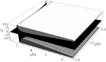
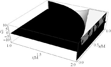
Figure 1: Angular momenta $\ell_{\mbox{\tiny{B}}}^{\pm}$ as function of radius $r/M$ and the spin-mass ratio $a/M$ of the spacetime. Right plot is a zoom in the ergoregion $r\in]r_{\epsilon}^{+},r_{+}[$. TIn the shadded regions the effective potential function $V_{eff}^{2}$ is not defined. White surface is the plane $\ell_{\mbox{\tiny{B}}}^{\pm}=0$, $\ell_{\mbox{\tiny{B}}}^{+}<\ell_{\mbox{\tiny{B}}}^{-}$ is the gray surface. The horizon $r_{+}$ and the static limit are also plotted (black surfaces).

where $\Delta^{\pm}_{\ell}(a)\equiv\ell\pm a$ and $\left.r_{\mbox{\tiny{B}}}^{\pm}\right|_{\ell=\pm a}=0$, Fig. (1). It is on the other hand:

$$\left.V_{eff}(\ell)\right|_{\ell=a}=\sqrt{\frac{\Delta}{r^{2}}},\quad\left.V_{eff}(\ell)\right|_{\ell=-a}=\sqrt{\frac{r\Delta}{8Ma^{2}+r^{3}}},$$ (19)

the effective potential at $\ell=\pm a$ is therefore well defined in all $r>r_{+}$. The limiting case of $a=0$ has been addressed in PuMonBe12 , and for the extreme Kerr-BH case it is in particular:

$$\mbox{{Extreme Kerr case:}}\quad a=M,\quad\ell/M=-7\quad\mbox{and}\quad r>M-\{r=4M\},$$ (20)

$$\ell\in]-7M,2M[\quad\mbox{and}\quad r>M,$$

$$\ell/M<-7\cup\ell/M>2\quad\mbox{and}\quad r\in]r_{+},r_{\mbox{\tiny{B}}}^{-}[\cup]r_{\mbox{\tiny{B}}}^{+},\infty[.$$

More generally for spacetime spins $a\in]0,M]$ and on any plane $\sigma\in]0,1]$, the fluid effective potential is well defined in:

$$r\in]r_{+},r_{\epsilon}^{+}[\quad\mbox{for}\quad\ell<\ell_{\sigma}^{-},\quad\mbox{at}\quad r=r_{\epsilon}^{+}\quad\mbox{for}\quad\ell<\frac{\left(a^{2}+r^{2}\right)^{2}-a^{2}\Delta\sigma^{2}}{4aMr};\quad\mbox{and in}\quad r>r_{\epsilon}^{+}\quad\mbox{for}\quad\ell\in]\ell_{\sigma}^{-},\ell_{\sigma}^{+}[,$$

with

$$\ell_{\sigma}^{\pm}\equiv\frac{2aMr\sigma^{2}}{2Mr-\rho^{2}}\pm\sqrt{\frac{\Delta\rho^{4}\sigma^{2}}{\left(\rho^{2}-2Mr\right)^{2}}},\quad\left.\ell_{\sigma}^{\pm}\right|_{\sigma=1}=\ell_{\mbox{\tiny{B}}}^{\pm}.$$ (21)

The conditions above arise from: $V_{eff}(\ell)^{2}=U_{t}^{2}>0$, as such they regulate some aspects of the hydrodynamics of the system but do not define the toroidal P-D topology as they are indeed necessary but not sufficient conditions for a P-D accretion disk could be formed. To obtain this we should analyse the critical points of the effective potential function $V_{eff}(\ell)$. However equations  (15,16) and (18), reveal that the regions where a fluid configuration can be formed, as regulated by Eqs. (12), depend on $\Delta_{\ell}^{\pm}(a)=\ell\pm a$. Considering that the configurations can be counterrotating $(\ell<0)$ and rotating $(\ell>0)$, as seen from Eqs. (15,16), there is a significant difference, in terms of fluid angular momenta, between the regions $r>r_{\epsilon}^{+}$ and $r\in]r_{+},r_{\epsilon}^{+}[$. The structure of these regions outside the static limit ($r>r_{\epsilon}^{+}$ on $\theta=\pi/2$) coincides qualitatively with that of the non rotating case $a=0$ where $r_{+}=r_{\epsilon}^{+}$. Indeed, the upper limit $\ell_{lim}$ of the angular momentum for $r=r_{\epsilon}^{+}$ diverges as $a$ approaches zero, and has the limiting values $\ell_{lim}/M=3$ as $a=M$. The limit $\ell_{lim}(a)$ is a monotonically decreasing function of $a/M$, this implies that the range of angular momentum for corotating fluid approaching the static limit decreases with the black hole spin. Finally the behaviour of the boundaries $\ell_{\mbox{\tiny{B}}}^{\pm}$ is very complicated as these are function of $(a,r)$, however, in the region $r>r_{\epsilon}^{+}$ there is a minimum of the $\Delta_{\ell_{\mbox{\tiny{B}}}}=|\ell_{\mbox{\tiny{B}}}^{+}-\ell_{\mbox{\tiny{B}}}^{-}|$ and then $\Delta_{\ell_{\mbox{\tiny{B}}}}$ increases with $a/M$ Fig. (1).

III.2 Analysis of the fluid configurations and pressure-free case

Many phases of the accretion process in the P-W scheme are regulated by the proprieties of the effective potential function on the equatorial plane. We use this property extensively confining our analysis mostly to a survey on the equatorial plane of symmetry, projecting each functions on $\theta=\pi/2$. We investigate the orbital regions where a P-D fluid configuration exist studying the effective potential critical points on the equatorial plane, in particular we focus on the relation with the potential $V_{eff}(L)$ for case of negligible pressure. The critical points of the potential $V_{eff}(\ell)$ are related to the critical points of the potential $V_{eff}(L)$ for the Keplerian disk by the following relation:

$$\partial_{r}V_{eff}(\ell)=\partial_{r}V_{eff}(L)+\partial_{L}V_{eff}(L)\partial_{r}L(\ell)=0.$$ (22)

On the other hand, in the regions where $p=0$ it is $\Sigma_{L}\equiv\Sigma_{\ell}$. In general one can say: open $\left({O}\right)$ configurations are for $K>1$, closed $\left({C}\right)$ disks for $K\in]0,1[$. There can be crossed surfaces $\left(O_{x},C_{x}\right)$ for each classes as the effective potential has a maximum, that is a minimum of the hydrostatic pressure, the maximum of pressure on the other hand (minimum of $V_{eff}(\ell)$) are associated to the center of the disk. Note that $\partial_{L}V_{eff}(L)=0$ at $r>r_{\epsilon}^{+}$ for every $a\in]0,1]$ and $\bar{\bar{L}}/M\equiv-2\sqrt{{a^{2}}/{(r-2M)r}}$ ($r=M+M\sqrt{{(4a^{2}+L^{2})/(L^{2})}}$), where $L$ must be negative and it is $\bar{\bar{L}}\neq-L_{+}$. The fluid angular momentum, solutions of Eq. (22) are

$$\ell_{f}^{\pm}:\;\partial_{r}V_{eff}(\ell_{f}^{\pm})=0,\quad\frac{\ell_{f}^{\pm}}{M}\equiv\frac{a^{3}+ar(3r-4M)\pm\sqrt{r^{3}\Delta^{2}/M}}{a^{2}M-(r-2M)^{2}r},\quad\mbox{at}\quad\sigma=1,$$ (23)

in the Schwarzschild and the extreme BH cases it is respectively

$$\left.\ell_{f}^{\pm}\right|_{a=0}=\pm\frac{Mr^{4}}{\sqrt{(r-2M)^{2}Mr^{5}}},\quad\left.\ell_{f}^{\pm}\right|_{a=M}=\frac{M^{3}\pm M^{3}\sqrt{r^{3}/M^{3}}-rM^{2}\left(3\pm\sqrt{r^{3}/M^{3}}\right)}{r(r-3M)+M^{2}}.$$ (24)

where $\ell_{f}^{-}>0$, $\forall r>r_{+}-\{r_{d}\}$, and $\ell_{f}^{+}>\ell_{f}^{-}>0(\ell_{f}^{+}<0)$ for $r\in]r_{+},r_{d}[(]r_{d},\infty[)$, moreover it is

$$r_{d}\equiv\frac{8M}{3}\cos\left[\frac{1}{6}\arccos\left(\frac{27a^{2}}{16M^{2}}-1\right)\right]^{2},\quad\ell_{f}^{\pm}(r_{\epsilon}^{+})=\frac{4M^{2}}{a}+a\pm 2M\sqrt{2},\quad\lim_{r\rightarrow r_{\pm}}\ell_{f}^{+}=\lim_{r\rightarrow r_{\pm}}\ell_{f}^{-}=\frac{2Mr_{\pm}}{a},$$ (25)

with

$$r_{d}(\check{a})=r_{lsco}^{-}(\check{a})\approx 2.54257M,\quad\breve{a}\equiv\frac{1}{3}\sqrt{\frac{1}{2}\left(249-41\sqrt{33}\right)}M\approx 0.865157M,$$

the solution $r_{d}(a,M):a^{2}M-(r-2M)^{2}r=0$ from Eq. (23) is plotted in Fig. (2) with the $r_{\gamma}^{\pm}$ and $r^{\pm}_{lsco}$. We consider then the set of orbits $\mathfrak{R}\equiv\{r_{d},r_{\epsilon}^{+},r_{lsco}^{\pm},r_{b}^{\pm},r_{\gamma}^{\pm}\}$, and the spin set $\mathfrak{A}\equiv\{a_{\circ},a_{\bullet},a_{\flat},a_{{\dagger}},a_{\Box},a_{\diamondsuit},{\check{a}},a_{\natural}\}$ associated with the orbits in $\mathfrak{R}$ each spin is shown in Fig. (2) as the cross between pairs of orbits $r_{i}\in\mathfrak{R}$.

Furthermore, we can express conditions in Eqs. (15,16) in terms of the fluid angular momentum and the limiting photon orbits $r_{\gamma}^{\pm}$ as follows:

Kerr case $$a\in]0,M[$$: (26)

$$\ell<\ell_{\gamma}^{+}\cup\ell\in]\ell_{\gamma}^{-},\ell_{f}^{-}(r_{+})[\cup\ell>\ell_{f}^{-}(r_{+})\quad\mbox{and}\quad r\in]r_{+},r_{\mbox{\tiny{B}}}^{-}[\cup]r_{\mbox{\tiny{B}}}^{+},\infty[,$$

$$\ell\in]\ell_{\gamma}^{+},\ell_{\gamma}^{-}[\quad\mbox{and}\quad r>r_{+},\quad\ell=\ell_{f}^{-}(r_{+})\quad\mbox{and}\quad r>r_{\mbox{\tiny{B}}}^{+},$$

$$\ell=\{\ell_{\gamma}^{+},\ell_{\gamma}^{-}\}\quad\mbox{and}\quad r>r_{+}-\{r_{\mbox{\tiny{B}}}^{+}\},$$ (27)

see Fig. (1) where

$$\ell_{\gamma}^{\pm}\equiv\ell_{f}^{\pm}(r_{\gamma}^{\pm})=-\frac{a}{M}\mp 6\cos\left[\frac{\arccos\left(\pm\frac{a}{M}\right)}{3}\right],$$ (28)

more generally we introduce the notation $\mathbf{Q}_{b}^{\pm}\equiv\mathbf{Q}(r_{b}^{\pm})$ and also $\mathbf{Q}_{lsco}^{\pm}\equiv\mathbf{Q}(r_{lsco}^{\pm})$, for any quantity $\mathbf{Q}$ as well. The angular momentum of the test particles orbits and the fluid angular momentum in the P-D configurations are related as follows: $\ell_{f}^{+}=\frac{-L_{+}}{E_{+}}$ and $\ell_{f}^{-}=\frac{L_{-}}{E_{-}}$,where $\ell_{L}^{\pm}(L_{\pm})=\ell_{f}^{\mp}$ and $L\left(l_{f}^{\pm}\right)=L_{\pm}$ with the definitions Eqs. (13), and $l_{f}^{\pm}:\;\left.\partial_{r}L(\ell)\right|_{\ell_{f}^{\pm}}=0$, that is the fluid angular momentum under hydrostatic pressure are the critical points of the angular momentum for test particle motions $L(\ell)$ respect to the radial coordinate, precisely taking into consideration the existence conditions Eqs. (27) the critical points are

$$\mbox{for}\;a\in[0,a_{\flat}]: \mbox{in}\;r\in]r_{\gamma}^{-},r_{\gamma}^{+}]\mbox{with}\ \ell_{f}^{-},\quad\mbox{and}\quad r>r_{\gamma}^{+},\;\mbox{with}\quad\ell_{f}^{\pm},\quad a_{\flat}\equiv\frac{1}{3}\sqrt{\frac{7}{3}}M\approx 0.509175M,$$ (29)

$$\mbox{for}\;a\in]a_{\flat},M]: \mbox{in}\;r\in]r_{\gamma}^{-},r_{d}[,\;\mbox{with}\;\ell_{f}^{-}\;\mbox{and}\;r=r_{d}\;l=\ell_{d},\;\mbox{in}\;r\in]r_{d},r_{\gamma}^{+}]\;\mbox{with}\;\ell_{f}^{-},\quad r>r_{\gamma}^{+}\;\mbox{with}\;\ell_{f}^{\pm}.$$ (30)

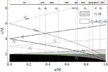
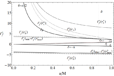
Figure 2: Left panel: Radii of the set $\mathfrak{R}\equiv\{r_{d},r_{\epsilon}^{+},r_{lsco}^{\pm},r_{b}^{\pm},r_{\gamma}^{\pm}\}$ as function of black hole spin-mass ratio $a/M$, namely the last circular orbit for time-like particles $r_{\gamma}^{\pm}$, the last bounded orbit is $r_{b}^{\pm}$, and the last stable circular orbit is $r_{lsco}^{\pm}$, where $(\pm)$ is for counterrotating or corotating orbits with respect to the attractor on the equatorial plane $\theta=\pi/2$. The outer horizon $r_{+}/M$, and the static limit $r_{\epsilon}^{+}=2M$, and $r_{d}$, are also plotted, the regions of positive fluid angular momentum $\ell_{f}^{\pm}$, for counterrotating and corotating fluid are shadded. The gray region is $]r_{\epsilon}^{+},r_{+}[$, the black region $r<r_{+}$. Vertical lines are the spin in $\mathfrak{A}\equiv\{a_{\circ},a_{\bullet},a_{\flat},a_{{\dagger}},a_{\Box},a_{\diamondsuit},{\check{a}},a_{\natural}\}$ where: $a_{\circ}\equiv(8\sqrt{2}-11)M$, $a_{\bullet}\equiv(23-16\sqrt{2})M$, $a_{\flat}/M\equiv{\sqrt{{7}/{3}}}/{3}$, $a_{{\dagger}}/M\equiv{1}/{2}\left(3\sqrt{17}-11\right)M$, $a_{\Box}\equiv 1/{\sqrt{2}}M$, $a_{\diamondsuit}\equiv 2\left(\sqrt{2}-1\right)M$, $\check{a}\equiv 0.865157M$, $a_{\natural}\equiv 2\sqrt{2}/3M$. Nice classes of black hole spacetimes, $\mathbf{BHI-IX}$, are outlined. Right plot: fluid angular momentum $\ell^{\pm}_{f}$ of the orbits in units of mass $M$ of $\mathfrak{R}$ as function of $a/M$.

III.2.1 On the fluid angular momentum

Some notes on the counterrotating configurations The fluid momentum associated with the counterrotating configurations is $\ell_{f}^{+}$: counterrotating disks can be formed only at $r>r_{\gamma}^{+}>r_{d}>r_{\epsilon}^{+}$, where $\ell_{f}^{+}$ sets the critical points of the fluid effective potential as function of the radius $r$. The case $\ell=0$ is not a value for $\ell_{f}^{\pm}$ and it is not a critical point for the effective potential $V_{eff}(\ell)$ (for $\sigma\in[0,1]$), we could say there is no continuum sequence of configurations, parameterized by $\ell$, from the corotating $(\ell>0)$ to the counterrotating $(\ell<0)$ fluids. On the orbit $r=r_{d}$, $\ell_{f}^{\pm}$ are not well defined, however the pressure has still a critical point, the associated angular momentum is:

$$l_{d}=\left.\frac{a^{4}+2a^{2}(r-2M)r+r^{4}}{2a\left[a^{2}+r(3r-4M)\right]}\right|_{r_{d}}>0,\quad a\neq a_{\flat},$$ (31)

where $\ell_{f}^{-}$ approaches $\ell_{d}$ in the limit $r\approx r_{d}$, Fig. (3). The function $\ell_{d}>0$ can be seen as a “transition” fluid angular momentum and $r_{d}:\;\ell_{f}^{+}\lessgtr 0$ for $r\gtrless r_{d}$ as a “transition” orbit Fig. (3): the critical points at $(r_{d},\ell_{d})$ exist only in the spacetimes $a\in]a_{\flat},M]$, where $V_{eff}(r_{d},\ell_{d})=1$ as $a$ increases and it goes to infinity as $a=a_{\flat}$, precisely it is $K>1$ in $a\in]a_{\flat},a_{{\dagger}}[$, $K=1$ for $a=a_{{\dagger}}$, $K\in]0,1[$ in the spacetimes $a\in]a_{{\dagger}},M]$, where $a_{{\dagger}}\equiv{1}/{2}\left(3\sqrt{17}-11\right)M:\;r_{b}^{-}(a_{{\dagger}})=r_{d}(a_{{\dagger}})$. The effective potential is well defined at $\ell<0$ in the ergoregion (at any plane) but has no critical points for $\ell<0$. Then, it is $\ell_{f}^{+}<0$ when $L_{+}\lessgtr 0$ and $E_{+}\lessgtr 0$, however the positive solutions $\ell_{f}^{+}$ can exist for $r\in]r_{+},r_{d}[$ but both $L_{+}$ and $E_{+}$ are well (real) defined when $r>r_{\gamma}^{+}$, moreover in the BH-case there are no circular orbits with $E<0$ and $(L_{+},E_{+})$ are positive and defined for $r>r_{\gamma}^{+}$. In $r\in]r_{+},r_{d}[$ the couple $(E_{-},L_{-})$ is well defined and it is $\ell_{f}^{-}=L_{-}/E_{-}$, then it is $r_{d}(a_{\flat})=r_{\gamma}^{-}(a_{\flat})$, at $r<r_{\gamma}^{-}$ no circular orbits with $L_{-}$ are possible, it is $r_{d}(\check{a})=r_{lsco}^{-}(\check{a})$.

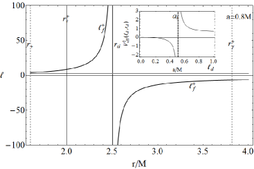
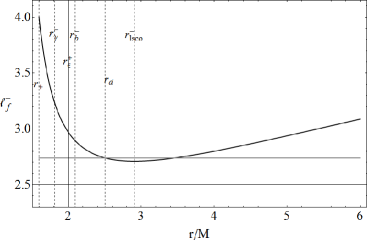
Figure 3: Left panel: spacetime spin $a=8/10M\in\mathbf{BHVI}$, fluid angular momentum in units of mass $M$, $\ell_{f}^{+}$ (black curve), $\ell_{d}=2.74035M$ (gray curve) as functions of $r>r_{+}$, the horizon $r_{+}=1.6M$ and the static limit $r_{\epsilon}^{+}=2M$ are plotted (dashed lines). The inset plot is the effective potential $V^{2}_{eff}(\ell_{d},r_{d})$ function of $a/M$. The energy function $V^{2}_{eff}(\ell_{d},r_{d})$ is not well defined in $a=a_{\flat}\approx 0.51M$ and it is negative in $a<a_{\flat}$. Right panel: spacetime spin $a=8/10M\in\mathbf{BHVI}$, fluid angular momentum $\ell_{f}^{-}$ for corotating matter as function of $r/M$. Dashed lines are the last circular orbit $r_{\gamma}^{-}$, the static limit $r_{\epsilon}^{+}$, and the last bounded orbit $r_{b}^{-}$, the radius $r_{d}$, and the last stable circular orbit $r_{lsco}^{-}$. The curve $\ell_{f}^{-}>0$ spacetime spin $a=8/10M\in\mathbf{BHVI}$ has a minimum point in $r_{lsco}^{-}$.

This analysis however does not specify the configuration topology, in order to do this we need to study Eq. (22) by taking a second derivation with respect to $r$ and to consider the values of the parameter $K\in[0,\infty[$ to establish the possible existence of a cusp and to fix the $({O},{C})$ classes.

Orbital regions of extreme fluid angular momentum We investigate the critical points of the fluid angular momentum i.e. the solutions of $\left.\partial_{r}\ell_{f}^{\pm}\right|_{\theta=\pi/2}=0$. These orbits are related to the orbits of maximum and minimum particle angular momentum regulating the case of the Keplerian disks or null pressure $p$ configuration, see Figs. (2)-right.

On the counterrotating fluid angular momentum The angular momentum for counterrotating fluids $\ell^{+}_{f}<0$ increases with the the orbital distance from the center i.e. $\partial_{r}\ell_{f}^{+}>0$, in $r\in]r_{+},r_{\epsilon}^{+}]$. Critical points of the fluid angular momentum on the equatorial plane exist in $r\in[6M,9M]$, on $r=r^{+}_{lsco}$, line of saddle points for the effective potential, as $a/M$ varies in $[0,1]$ see Figs. (2)-left, from the case at $a=0$ in $r_{lsco}^{+}=6M$ to $a=M$, $r_{lsco}^{+}=9M$. The counterrotating angular momentum increases with the radius in $]r_{+},r_{lsco}^{+}[-\{r_{d}\}$ that is in $r\in]2M,6M[$, while the angular momentum decreases always with the radius (on the equatorial plane) far enough from the attractor i.e. $r>9M$ and in general in $r>r_{lsco}^{+}$. However there are no turning points or minimum for the specific fluid momentum but there is a maximum point at $\left.\ell_{f}^{+}\right|_{\mbox{\tiny{Max}}}$ as it is $\partial_{r}^{2}\ell_{f}^{+}<0$ on the orbit $r_{lsco}^{+}$. The maximum value $\ell^{+}_{f}(r_{lsco}^{+})$ is plotted in Fig. (2) for $a\in[0,M]$.

The corotating fluid angular momentum The critical points of the angular momentum $\ell_{f}^{-}$ are in the range $r\in]M,6M]$, in particular for $a=0$ in $r=6M$ and at $a\in]0,\check{a}[$ at $r=r_{lsco}^{-}$. It is $\partial_{r}\ell_{f}^{-}>0$ in $r>6M$, for any attractor with $a/M\in[0,1]$, but in the case of a Schwarzschild geometry ($a=0$) increases in $r>6M$ and $a\in]0,\check{a}]$ in $r>r_{lsco}^{-}$ and for sources $a\in]\check{a},M]$ in $r>r_{lsco}^{-}-\{r_{d}\}$. There are minimum points at $r_{lsco}^{-}$. The angular momenta $\ell_{lsco}^{\pm}$ decrease with $a/M$, see Figs. (2). It is worth noting that there is a region of minimum points in the ergoregion as $a\in]a_{\natural},M]$ where at $a_{\natural}\equiv 2\sqrt{2}/3M$ it is $r_{lsco}^{-}(a_{\natural})=r_{\epsilon}^{+}$. Nevertheless it is always $K<1$ on these peculiar orbits, that means the possibility for $C$ configuration to form, see Fig. (4).

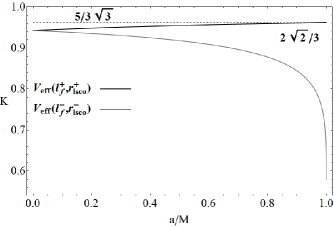
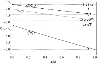
Figure 4: Left top panel: plot of the effective potential $V_{eff}(\ell_{f}^{\pm},r_{lsco}^{\pm})$ as function of $a/M$. At $a=M$ the $r_{lsco}^{-}$ reaches the horizon. Right top and bottom panels angular momentum, in units of mass $M$, $\ell_{f}^{-}$ $(\ell_{f}^{+})$ at $\{r_{lsco}^{-},r_{b}^{-},r_{\gamma}^{-}\}$, $(r_{lsco}^{+},r_{b}^{+},r_{\gamma}^{+})$ for different spacetimes. It is $\ell_{f}^{\mp}(r_{\gamma}^{\mp})\gtrless\ell_{f}^{\mp}(r_{b}^{-})\gtrless\ell_{f}^{\mp}(r_{lsco}^{\mp})$. In terms of the fluid angular momentum only ${C}_{x}$ configurations are at $K<1$ and $\ell\in]\ell_{b}^{+},\ell_{lsco}^{+}[$ and $\ell\in]\ell_{lsco}^{-},\ell_{b}^{-}[$, ${C}$ disks are for $K\in]K_{lsco}^{\pm},1[$, $\ell<\ell_{lsco}^{+}<0\cup\ell>\ell_{lsco}^{-}>0$ and $r>r_{lsco}^{\pm}$, ${O}_{x}$ disks at $K>1$ $\ell\in]\ell_{\gamma}^{+},\ell_{b}^{+}[\cup]\ell_{b}^{-},\ell_{\gamma}^{-}[$, see text.

III.3 Classes of Kerr attractors and disks configurations

In this section we investigate the existence of the thick configurations with angular momentum $\ell=\ell_{f}^{\pm}$ considering separately the following three cases: (I)$K>1$, (II) $K=1$, (III) $K\in]0,1[$, where opened $\left({O}\right)$ configurations are for $K>1$, closed $\left({C}\right)$ for $K\in]0,1[$. For each classes, $(O,C)$ there can be crossed surfaces or $(O_{x},C_{x})$, where the hydrostatic pressure is minimum and the accretion can occur. P-D configurations can exist in $r>r_{\gamma}^{\pm}$ with $|\ell|<|\ell_{f}(r_{\gamma}^{\pm})|$ for counterrotating or corotating matter respectively. We detail the situation as follows. (I) for $K>1$ there are only maximum points for the effective potential on $r=r_{f}^{\pm}$ solutions $r_{f}^{\pm}:\;a^{2}M(\Delta_{\ell}^{-})^{2}-4M^{3}(\Delta_{\ell}^{-})^{2}r+2M(\Delta_{\ell}^{-}+\ell)(\Delta_{\ell}^{-})r^{2}-\ell^{2}r^{3}+Mr^{4}=0$ correspondingly there are ${O}_{x}$-configurations only with: $\ell\in]\ell_{\gamma}^{+},\ell_{b}^{+}[\cup]\ell_{b}^{-},\ell_{\gamma}^{-}[$. These configurations fill the orbital regions $r\in]r_{\gamma}^{\pm},r_{b}^{\pm}[$ closest to the attractor, these can be accretion points. (II) for $K=1$ there are only maximum points of $V_{eff}(\ell)$, thus ${O}_{x}$-configurations, on $r_{b}^{\pm}$ with $\ell_{f}(r_{b}^{\pm})$ respectively. (III) for $K\in]0,1[$ the fluid is characterized by maximum, minimum or saddle points for the effective potential. For $K\in]K_{lsco}^{\pm},1[$ the minimum points, centers of ${C}$-configurations, are in $r>r_{lsco}^{\pm}$ with $\ell<\ell_{lsco}^{+}<0\cup\ell>\ell_{lsco}^{-}>0$. The maximum points of the effective potential with $K<1$ (minima of the pressure as function of the orbital distance from the source) are associated to the closed crossed, ${C}_{x}$ surfaces with the angular momentum $\ell\in]\ell_{b}^{+},\ell_{lsco}^{+}[$ and $\ell\in]\ell_{lsco}^{-},\ell_{b}^{-}[$, the radius of these orbits, location of the accretion points, are at $r_{f}^{\pm}\in]r_{b}^{\pm}r_{lsco}^{\pm}[$. As the $C$-disk is formed, it can thicken approaching the source, leading to the $C_{x}$-accretion morphology, and eventually it could rise in the unstable modes with open branches as $O_{x}$, thus one could say that the disk follows, during its evolution the sequence of configurations $\mathfrak{B}=[C,C_{x},O_{x}]$. One can argue that the entire evolution of a P-D disk, from the formation to the accretion and finally to the open configuration (or reversing with an excretion process see for example 2011 ; astro-ph/0605094 ; Stu-Sla-Hle:2000:ASTRA: ; arXiv:0910.3184 ) could occur for example as one of the following sequences of P-D configurations: $\mathfrak{B}=[{C},{C}_{x},{O}_{x},{O}]$ (or even $\mathfrak{B}=[{O},{O}_{x},{C}_{x},{C}]-[{C}_{x},{C}]$). The configurations in the sequence $\mathfrak{B}$ are all Boyer surfaces, correspondent to the pressure critical points, however the dynamical evolution between each configurations of $\mathfrak{B}$, is due to a (correlated) change of the model parameters $\mathbf{p}\equiv(K,\ell)$, the transition configurations between one Boyer surface to another of the sequence $\mathfrak{B}$ represents a transition in the dynamical evolution of the disks interacting with the external environment. This evolution can be clearly followed through the shifting of the effective potential and therefore the $K$-parameter, this aspect will be investigated in details in Sec. (III.3). As it is $r_{\gamma}^{-}>r_{\gamma}^{+}$, corotating and counterrotating thick disks can be in, or share part of the same orbital region. Here we construct a set of corotating and counterrotating configurations keeping one parameter of the couple $\mathbf{p}\equiv(K,\ell)$ constant and changing the other one in the set of values for the formation of a P-D surface. We consider then the set of orbits $\mathfrak{R}\equiv\{r_{d},r_{\epsilon}^{+},r_{lsco}^{\pm},r_{b}^{\pm},r_{\gamma}^{\pm}\}$: correspondingly the regions between subsequent orbits of $\mathfrak{R}$ identify a slot of the sequence $\mathfrak{B}$. The properties of the P-D configurations turn out to be so distinctive that they allow the introduction of a complete classification of Kerr spacetimes according to the spin set $\mathfrak{A}\equiv\{a_{\circ},a_{\bullet},a_{\flat},a_{{\dagger}},a_{\Box},a_{\diamondsuit},{\check{a}},a_{\natural}\}$ as shown in Fig. (2), each class is characterized by different physical features of the thick disks that could be of particular relevance in observational astrophysics. We locate nine classes of Kerr attractors, named accordingly $\mathbf{BHI-BHIX}$ and identifiably in terms of their spin mass ratio class in the ranges with boundaries in $\mathfrak{A}$ as illustrated in Fig. (2). Each class has different characteristics in the arrangement of the Boyer surfaces and therefore in their possible evolution between one configuration to another. As a consequence of this the analysis of the toroidal configurations could be a possible way to recognize a source from the analysis of the toroidal configuration and in particular the fluid angular momentum. In the following we define each class of attractors discussing their main properties in terms of the characteristic sequence $\mathfrak{B}$.

The BHI class: ${a\in[0,a_{\circ}]}$

It is $a_{\circ}\equiv(8\sqrt{2}-11)M$ where $r_{b}^{-}(a_{\circ})=r_{\gamma}^{-}(a_{\circ})$, this class of metrics includes the special case of the Schwarzschild geometry. In general in the BHI spacetimes the orbits $r_{i}\in\mathfrak{R}$ can be ordered as follows: $r_{lsco}^{+}>r_{lsco}^{-}>r_{b}^{+}>r_{b}^{-}>r_{\gamma}^{+}>r_{\gamma}^{-}>r_{d}>r_{\epsilon}^{+}>r_{+}$. The set of possible configurations is $\mathfrak{B}_{I}\!=\![C^{\pm},(C^{-}C^{+}_{x}),C_{x}^{\pm},(C_{x}^{-}O_{x}^{+}),O_{x}^{\pm},O_{x}^{-}]$, each of the six slot of $\mathfrak{B}_{I}$ is associated to one of the six regions $[r_{i},r_{j}[$ with boundaries $r_{i}\in\mathfrak{R}$ where the hydrostatic pressure has critical points, and for ${a\in[0,a_{\circ}]}$ it includes the radii in $r>r_{\gamma}^{-}$. With $()^{\pm}$ we denote the disks of counterrotating or corotating fluids respectively, each slot of the six-dimension arrow $\mathfrak{B}_{I}$ is intended for a radial region where a couple or a single kind of configuration can be located starting from the region farthest from the source thus the farthest $C$ morphology to the closest $O_{x}$ one. Since each slot of $\mathfrak{B}_{I}$ identifies one of the regions in Fig. (2) determined by $\mathfrak{R}$, then the configuration $C_{x}$ are to be understood crossing two regions, the center of the configuration placed in the outer region, and the cross point in the inner one. The couple of different configurations in $\mathfrak{B}_{I}$ means a multiple configuration located in one orbital region, for example in $r>r_{lsco}^{+}$, they may both closed $C^{\pm}$ of corotating and counterrotating fluids but the spacing and the exact number of permitted disks, has to be further discussed and it will be addressed in Sec. (IV.5). The more we move towards the interior, that is, in regions closer to the attractor, and more unstable configurations appear leading to a transition from $C$ to $C_{x}$ up to $O_{x}$-configurations.

The BHII class: $a\in]a_{\circ},a_{\bullet}]$

It is $a_{\bullet}\equiv(23-16\sqrt{2})M$ where $r_{b}^{+}(a_{\bullet})=r_{lsco}^{-}(a_{\bullet})$. In these spacetimes it is $r_{b}^{-}>r_{\gamma}^{+}$, correspondingly $\mathfrak{B}_{II}\!=\![C^{\pm},(C^{-}C^{+}_{x}),C_{x}^{\pm},(C_{x}^{-}O_{x}^{+}),C_{x}^{-},O_{x}^{-}]$. Corotating surfaces are therefore allowed in a larger number of orbital regions respect to BHI geometries. Moreover there is a simultaneous decreasing of number of regions where both corotanting and counterrotating are possible, for example in this case as a consequence of the permutation between the couple $(r_{b}^{-},r_{\gamma}^{+})$ the double $O_{x}^{\pm}$ in BHI class is reduced to the $C_{x}^{-}$ configuration in BHII.

The BHIII class: ${a\in]a_{\bullet},a_{\flat}]}$

It is $a_{\flat}\equiv{\sqrt{{7}/{3}}}/{3}M$ where $r_{\gamma}^{-}(a_{\flat})=r_{d}(a_{\flat})$. Respect to the BHII geometries the BHIII spacetimes are characterized by a further permutation of the couple $(r_{lsco}^{-},r_{b}^{+})$ and it is $\mathfrak{B}_{III}\!=\![C^{\pm},(C^{-}C^{+}_{x}),(C^{-}O^{+}_{x}),(C^{-}_{x},O_{x}^{+}),C_{x}^{-},O_{x}^{-}]$. There is a reduction in the number of regions where $C_{x}^{+}$ are permitted, but the orbital extension in which these solutions are admitted increases with the spin. The difference with BHII spacetimes is the third slot of the sequences $(\mathfrak{B}_{II},\mathfrak{B}_{III})$, in $\mathfrak{B}_{III}$ filled with a corotating closed and open crossed counterrotating disks.

The BHIV class: $a\in]a_{\flat},a_{{\dagger}}]$

It is $a_{{\dagger}}/M\equiv{1}/{2}\left(3\sqrt{17}-11\right)M$ where $r_{b}^{-}(a_{{\dagger}})=r_{d}(a_{{\dagger}})$. Respect to the class BHIII there is a further permutation between $(r_{d},r_{\gamma}^{-})$. It is convenient to introduce the spin: $a_{{\ddagger}}\equiv 0.638284738M$ splitting the set $\mathbf{BHIV}$ as $\mathbf{BHIV}=\mathbf{BHIVa}\cup\mathbf{BHIVb}$. For BHIVa spacetimes it is $a<a_{{\ddagger}}$ and $\mathfrak{B}^{<}_{IV}\!=\![C^{\pm},(C^{-}C^{+}_{x}),(C^{-}O^{+}_{x}),(C_{x}^{-}O^{+}_{x}),C^{-}_{x},O_{x}^{-}]\equiv\mathfrak{B}_{III}$, and the orbital region of the last slot with $O_{x}^{-}$ configurations is crossed by $r_{d}$. For BHIVb spacetimes it is $a>a_{{\ddagger}}$, there is a permutation $(r_{\gamma}^{+},r_{lsco}^{-})$ and as a consequence it is $\mathfrak{B}^{>}_{IV}\!=\![{C}^{\pm},(C^{-}C^{+}_{x}),(C^{-}O^{+}_{x}),C^{-},C^{-}_{x},O_{x}^{-}]$.

The BHV class: $a\in]a_{{\dagger}},a_{\Box}]$

It is $a_{\Box}\equiv 1/{\sqrt{2}}M$ where $r_{\gamma}^{-}(a_{\Box})=r_{\epsilon}^{+}(a_{\Box})$ and $\mathfrak{B}_{V}\!=\mathfrak{B}^{>}_{IV}$. However respect to the BHIV geometries, in the spacetimes belonging to the BHV class there is the further permutation in the couple $(r_{d},r_{b}^{-})$, as of consequence of this the last slot of $\mathfrak{B}_{V}$, filled with $O_{x}^{-}$, and a part of $C^{-}_{x}$-region are now entirely contained in $r<r_{d}$.

The BHVI class: $a\in]a_{\Box},a_{\diamondsuit}]$

It is $a_{\diamondsuit}\equiv 2\left(\sqrt{2}-1\right)M$ where $r_{b}^{-}(a_{\diamondsuit})=r_{\epsilon}^{+}(a_{\diamondsuit})$, the sequence of configurations is $\mathfrak{B}^{>}_{VI}=\mathfrak{B}^{>}_{IV}$. For the spacetimes with spin $a>a_{\Box}$ there is a further permutation in the arrow $\mathfrak{R}$ involving the static limit $r_{\epsilon}^{+}$, for BHVI spacetime in particular there is a permutation in the couple $(r_{\gamma}^{-},r_{\epsilon}^{+})$: as a consequence of this the last slot of $\mathfrak{B}^{>}_{VI}$ filled with $O_{x}^{-}$ configurations, crosses the static limit and it is partially contained in $r<r_{\epsilon}^{+}$.

The BHVII class: $a\in]a_{\diamondsuit},{\check{a}}]$

It is $\check{a}\equiv 0.865157M$ where $r_{lsco}^{-}({\check{a}})=r_{d}({\check{a}})$. The sequence of configurations is $\mathfrak{B}_{VII}=\mathfrak{B}^{>}_{IV}$ and a permutation is in $(r_{d},r_{\epsilon}^{+})$, the region filled with the $O_{x}$ disks and a part of $C_{x}^{-}$ configurations are contained in the ergoregion.

The BHVIII class: $a\in]{\check{a}},a_{\natural}]$

It is $a_{\natural}\equiv 2\sqrt{2}/3M$ where $r_{lsco}^{-}(a_{\natural})=r_{\epsilon}^{+}(a_{\natural})$. The sequence of configurations is $\mathfrak{B}_{VII}=\mathfrak{B}^{>}_{IV}$. For these sources a further permutation occurs in the couple $(r_{d},r_{lsco}^{-})$, it follows that, respect to BHVII sources, a part of $C^{-}$ region is at $r<r_{d}$.

The BHIX class: $a\in]a_{\natural},M]$

The extreme black hole case is a special case of BHIX spacetimes. A further permutation respect to the situation in BHVIII geometries, is in the couple $(r_{lsco}^{-},r_{\epsilon}^{+})$ leading to the $C_{x}^{-}$ configuration entirely contained, and the $C^{-}$ configurations partially contained in the region $r<r_{\epsilon}^{+}$.

The limiting spacetimes with spin $a_{i}\in\mathfrak{A}$ require further investigation. In Secs. (III.3.1–III.3.3) we detail and comment the nine classes of attractors and the P-D torii, while the multiple configurations in the sequences $\mathfrak{B}$ will be discussed in Sec. (IV.5) and the P-D configurations near the static limit or in the region $r<r_{\epsilon}^{+}$, possible in the BHVI-IX spacetimes, are considered in details in Sec. (IV.1).

III.3.1 Configurations at $K=1$.

We consider the critical points of the effective potential for $K=1$, solutions of $V_{eff}(\ell)=K=1$ and $\partial_{r}V_{eff}(\ell)=0$. No minimum and saddle points are possible i.e. $\partial_{r}^{2}V_{eff}(\ell)\ngeq 0$. Maximum points are located on the orbits $r_{\kappa}^{-}$:

$$r_{\kappa}^{\pm}\equiv\frac{1}{4M}\left(\ell^{2}\pm\sqrt{-16\left(\frac{1}{4}l(4M+l)-aM\right)\left(\frac{1}{4}l(4M-l)-aM\right)}\right),$$ (32)

$$a\in[0,M[,\quad\ell=\{\ell_{b}^{+},\ell_{b}^{-}\},\quad a=M,\quad r=(3+2\sqrt{2})M\quad\ell=\ell_{b}^{+}.$$ (33)

On the other hand one can equally say orbits are in

$$a\in[0,M[-\{a_{{\dagger}}\},\quad r=r_{b}^{\pm}\quad\mbox{and}\quad\ell=\ell_{f}^{\pm},\quad\mbox{and}\quad a=\{a_{{\dagger}},a=M\}\quad\mbox{with}\quad\ell=\ell_{f}^{+}\quad\mbox{in}\quad r=r_{b}^{+}$$ (34)

$$a_{{\dagger}}\equiv\frac{1}{2}\left(3\sqrt{17}-11\right)M\approx 0.684658M,\quad r_{b}^{\pm}\equiv 2M\pm a+2\sqrt{M}\sqrt{M\pm a},$$

it is $a_{{\dagger}}:r_{b}^{-}=r_{d}$, and $r_{b}^{\pm}$ are the marginally bounded orbits for test particles: critical points of $r_{b}^{\pm}:\;\partial_{r}V_{eff}(r_{b}^{\pm},\mp L_{\pm})=0,\;\partial_{r}^{2}V_{eff}(r_{b}^{\pm},\mp L_{\pm})<0,\;V_{eff}(r_{b}^{\pm},\mp L_{\pm})=1$. There are open ${O}_{x}$ configurations. The surface $r_{\kappa}^{-}(a,\ell)$ includes the radii $r_{b}^{\pm}(a)$, where the cusps are located i.e. $\exists\ell(a):\;r_{\kappa}^{-}(a,\ell(a))=r_{b}^{\pm}(a)$, indeed it is: $r_{\kappa}^{-}(\ell_{b}^{\pm})=r_{b}^{\pm}$. Then there are two cusps correspondent to two different angular momenta for $a\neq 0$ and $a\neq M$, in the particular case of non-rotating attractor $a=0$ it is $r_{b}^{\pm}=4M$ and $\ell=\pm 4M$. In the spacetimes BHVII-IX these peculiar configurations of corotating fluids can fill the region $r<r_{\epsilon}^{+}$, see Fig. (2).

III.3.2 Configurations at $K\in]0,1[$.

We analyse the case $K\in]0,1[$ to find the maximum points of the effective potential ($\partial^{2}_{r}V_{eff}(\ell)<0$) associated to the cross points of the configurations ${C}_{{x}}$, and minimum points ($\partial^{2}_{r}V_{eff}(\ell)>0$) centers of the closed ${C}$-configurations. We will consider also the critical points $r_{f}:\ \partial_{r}V_{eff}(\ell)=0$, $\partial_{r}^{2}V_{eff}(\ell)=0$, saddle point and limiting orbits of instability. For the non rotating case of the Schwarzschild metric ($a=0$) minimum points are at $r>6M$ with $\ell=\pm\sqrt{\frac{Mr^{3}}{(r-2M)^{2}}}$. The maximum points are located in the lower orbital region $r\in]4M,6M[$. A saddle is located at $r=4M$, an extensive analysis of the non rotating background can be found in PuMonBe12 .

For a Kerr attractor ($a\in]0,1[$) we summarize the situation as follows:

Minimum points Minimum points of the effective potential $V_{eff}(\ell)$ are located in $r>r_{lsco}^{\pm}$. They are maximum points of the hydrostatic pressure and locate the disk center, and then with the instability points they contribute to determine the disk extension on the equatorial plane and the location of the inner boundary. However to analyze properly the minimum points we should consider two classes of sources, defined by the spins $\check{a}$: The first set is the BHI-VII classes where $a\in]0,\check{a}]$, and $\check{a}:\;r_{lsco}^{-}=r_{d}$; according with the analysis for the case of null pressure minimum points are located in $r\in]r_{lsco}^{-},r_{lsco}^{+}]$ with $\ell=\ell_{f}^{-}>0$, for corotating disk, and $r>r_{lsco}^{+}$ with $\ell=\ell_{f}^{\pm}$ where corotating and counterrotating disks are possible. Finally the second set is for $a/M\in]\check{a},M[$-BHVIII-IX. Minimum points are located in $r\in]r_{lsco}^{-},r_{d}[$ with $\ell=\ell_{f}^{-}>0$ for corotating disks, $(r=r_{d},\ell=\ell_{d})$, at $r\in]r_{d},r_{lsco}^{+}]$ with $\ell=\ell_{f}^{-}$, and $r>r_{lsco}^{+}$ with $\ell=\ell_{f}^{\pm}$. Counterrotating closed disks (minimum points) are possible only at $r>r_{lsco}^{+}$. The angular momentum $\ell_{f}^{-}$ has a bounded orbital extension and penetrates the ergoregion at $a=a_{\natural}$ after that it extended theoretically up to the horizon. For BHVIII sources with $a\in]\check{a},a_{\natural}[$ the region with $\ell_{f}^{-}$ has the static limit as the upper bound, the region with $\ell_{f}^{-}$-tori within and out the ergoregion is then possible only for sufficiently large spin. The extension of the orbital region increases with the spin, up to the maximal extension for spin close to $a=M$. The transition orbit for the configurations here analyzed is instead $r_{lsco}^{+}$ that defines the lower boundary for the counterrotating fluids. However there are no critical points with $\ell=0$ for $K\in]0,1[$. This analysis can be then restated in terms of the orbits of minimum points, namely the orbits $r(a;\ell)$ where the minimum points are for $\ell<\ell_{lsco}^{+}<0\cup\ell>\ell_{lsco}^{-}>0$ at $r=r_{f}^{\pm}$ and in the non rotating case it is $\ell_{lsco}^{+}=-\ell_{lsco}^{-}=-3\sqrt{{3}/{2}}M.$ The solutions are $r_{f}^{\pm}:\;\ell_{f}^{\pm}=\ell$. From the analysis in Sec. (III.2.1) it follows that the angular momentum $\ell_{f}^{+}<0$ decreases with $r>r_{lsco}^{+}$.

The saddle, orbits $r_{f}$, are on the boundary $r_{lsco}^{\pm}$ where $\ell=(\ell_{lsco}^{+},\ell_{lsco}^{-})$.

Maximum points The maximum points of the effective potential with $K<1$ (minima of the pressure as function of the orbital distance from the source) are associated to the closed crossed ${C}_{x}$ surfaces located in the regions $r\in]r_{b}^{\pm},r_{lsco}^{\pm}[$. We consider the situations as follows:

1 for $a\in]0,a_{\bullet}[$-BHI-II-classes orbital regions are $r\in]r_{b}^{-},r_{b}^{+}]$ with $\ell=\ell_{f}^{-}$, and $r\in]r_{b}^{+},r_{lsco}^{-}[$ with $\ell=\ell_{f}^{\pm}$ and finally $r\in[r_{lsco}^{-},r_{lsco}^{+}[$ where $\ell=\ell_{f}^{+}$. In the spacetime with $a=a_{\bullet}$ it is in particular $r\in]r_{b}^{-},r_{b}^{+}[$ with $\ell_{f}^{-}$ and $r\in]r_{b}^{+},r_{lsco}^{+})$ with $\ell_{f}^{+}$.

2 for $a\in]a_{\bullet},a_{{\dagger}}]$-BHIII-IV classes it is $r\in]r_{b}^{-},r_{lsco}^{-}[$ with $\ell_{f}^{\pm}$ and $r\in]r_{b}^{+},r_{lsco}^{+}[$ with $\ell_{f}^{+}$. As for the case $p=0$, configurations at $\ell_{f}^{+}$ are counterrotating. However these orbits are in $r>r_{\epsilon}^{+}$. No torus configurations with $\ell=0$ are allowed.

3 for $a\in]a_{{\dagger}},\check{a}[$-BHV-VII-classes solutions are as follows $r\in]r_{b}^{-},r_{d}[$ with $\ell_{f}^{+}$, $r\in]r_{d},r_{lsco}^{-}[$ with $\ell_{f}^{-}$ and $r\in]r_{b}^{+},r_{lsco}^{+}[$ with $\ell_{f}^{+}$. For the spacetime $a=\check{a}$ it is $r\in]r_{b}^{-},r_{d}[\cup]r_{b}^{+},r_{lsco}^{+}[$ with $\ell_{f}^{+}$. In the spacetime with spin $a_{\lozenge}$ these orbits cross the static limit.

4 for $a\in]\check{a},M[$-BHVIII-IX-classes, maximum points are in $r\in]r_{b}^{-},r_{lsco}^{-}[$ with$\ell_{f}^{-}$ and $]r_{b}^{+},r_{lsco}^{+}[$ with angular momentum $\ell_{f}^{+}$. Interestingly for sufficiently high spin the first set of corotating orbits, located at $]r_{b}^{-},r_{lsco}^{-}[$ and $\ell_{f}^{-}>0$, are unstable and partly included in the ergoregion and there are indeed regions with both corotating and counterrotating matter.

Extreme BH case ($a=M$): In the extreme BH-case minimum points are in in $r\in]({M}/{2}),\left(3+\sqrt{5}\right)M[$ at $\ell=\ell_{f}^{-}$, in $r=\frac{1}{2}\left(3+\sqrt{5}\right)M$ at $\ell=\frac{1}{4}\left(7+\sqrt{5}\right)M$, and $r/M\in]\left(3+\sqrt{5}\right)/2,9]$ with $\ell=\ell_{f}^{-}$, and finally $r>9M$ with angular momentum $\ell=\ell_{f}^{\pm}$, i.e. $\ell<-22/5\cup\ell>2$ . Maximum points are in $r/M\in]5.82843,9[$ with $\ell_{f}^{-}$ that is $\ell/M\in]2\left(-1-\sqrt{2}\right),-{22}/{5}[$. On the other hand a saddle point is located at $r=9M$ with $\ell/M=-22/5$.

Range of the fluid angular momentum Maximum points of the effective potential are characterized by angular momentum $|\ell/M|\in]3\sqrt{{3}/{2}},4[$ for $a=0$, and for Kerr spacetime $a\in]0,M]$ it is $\ell\in]\ell_{b}^{+},\ell_{lsco}^{+}[$ and $\ell\in]\ell_{lsco}^{-},\ell_{b}^{-}[$.

At $r=r_{b}^{+}$, we need to introduce the spin $a_{\bullet}:\;r_{b}^{+}=r_{lsco}^{-}$: critical points are at $\ell_{f}^{-}$, maximum points are in the spacetimes $a\in]0,a_{\bullet}[$-BHI-II, minimum points are on $a\in]a_{\bullet},M]$-BHIII-IX and then a saddle point is on $a_{\bullet}$ $\ell=3.31081M$ and $r=4.71573M$.

Maximal extension of the $K$-parameter We introduce the notations: $K_{lsco}^{\pm}\equiv V_{eff}(\ell_{f}^{\pm},r_{lsco}^{\pm})$ and $K_{b}^{\pm}\equiv V_{eff}(\ell_{f}^{\pm},r_{b}^{\pm})$, see Figs. (4); the $K$ parameter lies in a bounded range $[K_{min},K_{Max}]\subset[0,+\infty[$. it is $K_{Max}=V_{eff}(\ell_{f}^{\pm},r_{b}^{\pm})=1$ and $K_{min}=V_{eff}(\ell_{f}^{\pm},r_{lsco}^{\pm})$. The boundary values depend on the spacetime spin, and they are different for counterrotating and corotating orbits: the $K^{-}_{lsco}$ ( for corotating fluids) decreases as the spacetime spin-mass ratio increases, on the contrary $K^{+}_{lsco}$ (for counterrotating fluids) decreases with $a/M$.

III.3.3 On the pressure critical points at $K>1$

Finally we consider the configurations defined by the conditions $V_{eff}(\ell)=K>1$, $\partial_{r}V_{eff}(\ell)=0$, this case is associated with the open configurations generally interpreted as hydrodynamics jets. There are no minimum or flexes, but there are maximum points on $r=r_{f}^{\pm}$, more precisely in a Kerr spacetime $a\in]0,1]$, maximum points are for: $\ell\in]\ell_{\gamma}^{+},\ell_{b}^{+}[\cup]\ell_{b}^{-},\ell_{\gamma}^{-}[\subset]-7,-4[\cup]2,3\sqrt{3}[$, The orbits $r_{f}^{\pm}$ cross the radius $r_{b}^{\pm}$ at $r=r_{b}^{-}$ for $\ell=l_{f}^{+}$ in the spacetimes $a/M\in]0,a_{\circ}[$-BHI, where $a_{\circ}:\;r_{b}^{-}=r_{\gamma}^{+}$. Or in terms of the fluid momentum $\ell_{f}^{\pm}$: maximum points for counterrotating fluid $(\ell_{f}^{+})$ are in the class BHI in the range $r\in]r_{\gamma}^{+},r_{b}^{+}[$ and in the classes $a\in]a_{\circ},M]$-BHII-III on $r\in]r_{\gamma}^{+},r_{b}^{+}[$. For corotating fluids $(\ell_{f}^{-})$ maximum points are in the BHI-III spacetimes where $a\in[0,a_{\flat}]$ in the range $r\in]r_{\gamma},r_{b}^{-}[$, and in the BHIV class with spin $a\in]a_{\flat},a_{{\dagger}}[$ in the range $r\in]r_{\gamma}^{-},r_{\gamma}^{+}[$ and $r\in]r_{\gamma}^{+},r_{b}^{-}[$, and finally for BHV-IX attractors where $a\in[a_{{\dagger}},M[$ in $r\in]r_{\gamma}^{-},r_{b}^{-}[$. For completeness we note here that the surfaces $K=V_{eff}=0$, are not critical points of the potential.

III.4 Analysis of the fluid configurations for the angular momentum $\bar{\ell}=\ell/a$

The orbital regions and the angular momentum where the effective potential $V_{eff}(\ell)$ is well defined depend on the difference $\Delta^{\pm}_{\ell}(a)\equiv\ell\pm a$ as in Eqs. (18), and one could introduce the rationalized dimensionless quantities $(r_{\mbox{\tiny{B}}}^{\pm}/a,\ell/a)$. More generally, many properties of the fluid effective potential are determined by the rationalized dimensionless quantity $\bar{\ell}\equiv\ell/(a\sigma^{2})$ where:

$$V_{eff}(\bar{\ell})=\sqrt{\frac{\Delta\rho^{2}}{r^{4}+a^{4}\left(\bar{\ell}^{2}-1\right)\left(\sigma^{2}-1\right)-a^{2}r\left[\bar{\ell}^{2}(r-2M)-2r+4M\bar{\ell}\sigma+(r-2M)\sigma^{2}\right]}},$$ (35)

and it is

$$\ell=-a\sigma^{2}\quad V_{eff}(\ell)=\sqrt{\frac{\Delta\rho^{2}}{\rho^{4}+8Ma^{2}r\sigma^{2}}},\quad\ell=a\sigma^{2}\quad V_{eff}(\ell)=\sqrt{\frac{\Delta}{\rho^{2}}},$$ (36)

see also Eq. (19). In the limiting case of the non-rotating Schwarzschild solution one could use the rationalized angular momentum $\bar{\ell}=\ell/\sigma$ to take into account, by means of the term $\sigma$, of the spherical symmetry of the spacetime PuMonBe12 , while for a rotating geometry we can consider $\bar{\ell}=\ell/\sigma^{2}$ only in the extreme-Kerr case $a=M$. In this section we study the P-D fluid configurations in terms on the rationalized parameter $\bar{\ell}\equiv\ell/a$. We show the existence of a limit on the maximum ratio $\bar{\ell}$ for the P-D model: in some cases the condition for the existence of these configurations is determined by the ratio $\bar{\ell}$ only. There are no critical points for $\bar{\ell}\in[-1,1]$ i.e. P-D configurations must have angular momentum whose magnitude is greater of the spacetime spin mass ratio, moreover also the momentum-spin ratio $\bar{L}\equiv L/a$, in the case of zero hydrostatic pressure or the Keplerian disk, is bounded to circular orbits with $|\bar{L}|>\mu$, see also discussion in ONeill95 ; chandra42 . However as the conditions $L(\ell)>a$ and $\ell\leq a$ cannot be fulfilled together, or $\ell(L)\in]-a,0[$ and $L>a$, as it is $\ell\equiv L/E$ (this quantity being related to the apparent impact parameter, of the light radii), then we could consider separately the orbits at $E/\mu>1$ (unbounded orbits) and $E/\mu\in(0,1)$ (bounded orbits), so that it will be convenient in the following to consider three classes of configurations. (I) Configurations with $K\in]0,1[$ The maximum extension of rationalized angular momentum at $r>r_{\epsilon}^{+}$, for the minimum points (torus centers) in the case of corotating fluids, is $\bar{\ell}>5-2\sqrt{2}$. There are no fluid configurations in the range $\bar{\ell}\in[1,2]$. Regarding the counterrotating configurations with minimum points (closed counterrotating torii), the angular momentum of the fluid is $\bar{\ell}<-22/5$ or $\ell<-3\sqrt{3/2}M$. For the saddle points of the fluid effective potential at $r>r_{\epsilon}^{+}$ it is $\bar{\ell}>5/2$ or $\ell/M\in]{5\sqrt{2}}/{3},3\sqrt{{3}/{2}}]$, and for the counterrotating configurations it is $\ell/M\in[-(22/5),-3\sqrt{3/2}]$, and $\bar{\ell}\leq-{22}/{5}$. Finally for the maximum points of the potential the maximum extension of the rationalized angular momentum outside the static limit is $\bar{\ell}>5/2$ where $\ell/M\in]{5\sqrt{2}}/{3},4[$. Regarding the counterrotating configurations with maximum points, the angular momentum of the fluid must be $\bar{\ell}<-22/5$ and $\ell/M\in]-2\left(1+\sqrt{2}\right),-3\sqrt{{3}/{2}}[$.

(II) Configurations with $K>1$ For $\ell>a$ only maximum points exist at $a/M\in[0,1[$ with $\ell/M\in]2,3\sqrt{3}[$, and $\bar{\ell}>2$. At $r>r_{\epsilon}^{+}$, it is $\bar{\ell}>1$ then $\bar{\ell}>2+\sqrt{2}$ and $\ell/M\in]2\sqrt{2},3\sqrt{2}[$. Counterrotating unstable configurations are characterized by $\ell/M\in]-7,-4[$ and $\bar{\ell}<2(-1-\sqrt{2})$.

(III) Configurations with $K=1$ For $K=1$ there are only maximum points. As $\ell>a$ maximum points are for $a\in[0,M[$ with $\ell=\ell_{b}^{-}$ and $r=r_{\kappa}^{-}$, where the angular momentum is limited in the range $\ell/M\in]2,4]$ and $\bar{\ell}>2$. For $\ell<-a$ there are only maximum points for $a\in[0,M]$ (note here is included the extreme Kerr case) and $\ell=\ell_{b}^{+}$ with $r=r_{\kappa}^{-}$, and $\ell/M\in[-2(1+\sqrt{2}),-4]$ and $\bar{\ell}\leq-2(1+\sqrt{2})$, out of the ergoregion. In conclusion corotating configurations with $K=1$ can exist only if $\bar{\ell}>2$ that is the fluid angular momentum doubles the black hole spin mass ratio, in the ergoregion these configurations can be formed only when $\bar{\ell}\in]2,2+\sqrt{2}[$. Counterrotating configurations can exist with the upper limit on the ratio $\bar{\ell}\leq-2(1+\sqrt{2})$.

IV Morphology of the Boyer surfaces and variation in the model parameters

In this section we study a more general class of matter configurations which includes the P-D torus as a special case. It is then convenient to analyze the zeros of the function $\mathcal{V}_{eff}(\mathbf{p})\equiv V_{eff}(\ell)-K$ on the equatorial plane i.e. we set $\sigma=1$ and $y=0$ as in the cartesian coordinates: $x=r\cos\theta$, $y=r\sin\theta$PuMonBe12 . Solutions on $\theta=\pi/2$, are at $y_{i}=y_{i}(a;\mathbf{p})$ with $i\in\{1,2,3\}$ and $K\neq 1$ where:

$$y_{1}=\frac{2M\left[\alpha_{\lambda}(K^{2}-1)\cos\left(\frac{1}{3}\arccos\beta_{\lambda}\right)-1\right]}{3(K^{2}-1)},\quad y_{2}=-\frac{2M\left[1+\alpha_{\lambda}(K^{2}-1)\sin\left[\frac{1}{6}(\pi+2\arccos\beta_{\lambda})\right]\right]}{3(K^{2}-1)},$$

$$y_{3}=-\frac{2M\left[1+\alpha_{\lambda}(K^{2}-1)\cos\left[\frac{1}{3}(\pi+\arccos\beta_{\lambda})\right]\right]}{3(K^{2}-1)},\quad\alpha_{\lambda}=\sqrt{\frac{4M^{2}+3(K^{2}-1)\left[K^{2}\Delta_{\ell}^{-}\Delta_{\ell}^{+}+a^{2}\right]}{M^{2}(K^{2}-1)^{2}}},$$

$$\beta_{\lambda}=-\frac{9(1-K^{2})\left[K^{2}\Delta_{\ell}^{-}\Delta_{\ell}^{+}+a^{2}\right]-8M^{2}-27K^{2}(K^{2}-1)^{2}(-\Delta_{\ell}^{-})^{2}}{\alpha_{\lambda}^{3}M^{2}(1-K^{2})^{3}},$$ (37)

$y_{i}$ are regulated by the difference $(K^{2}-1)$ and $\Delta_{\ell}^{\pm}$ introduced in Eq. (18), the particular solutions at $K=1$ will be discussed in Sec. (IV.4.2). In general there are three real solutions $y_{i}>0$ with $y_{2}<y_{3}<y_{1}$ , then the crossing points with the equatorial plane are represented for example with $y_{ijk}$ for the set $\{y_{i},\;y_{j},\;y_{k}\}$. We introduce here the quantities:

$$\ell_{\mu}^{\Pi}\equiv-2M+2\sqrt{M}\sqrt{M+a}<a,\;a\neq 0,\quad\ell_{a}^{1}\equiv-a+a\sin\left(\frac{\arcsin\frac{a}{M}}{3}\right)<0,$$ (38)

where in $]0,1[$ it is $-a<\ell_{a}^{1}<\ell_{\mu}^{\Pi}<a<\ell^{-}_{f}(r_{-})<\ell_{lsco}^{-}$ moreover it is $\ell_{f}^{\pm}(r_{+})\in]\ell_{f}^{-}(r_{\epsilon}^{+}),\ell_{f}^{+}(r_{\epsilon}^{+})[$, see also Fig. (2) and the quantities $K_{i}:\;i\in\{1,...,4\}$ are $V_{eff}(a;\ell,r_{f}^{\pm})$ where $r_{f}^{\pm}(a;\ell):\;\ell_{f}^{\pm}(a,r)=\ell$. The zeros of $\mathcal{V}_{eff}(\mathbf{p})$ ($\Sigma_{{V}_{eff}}$ surfaces) include but do not reduce to the critical values of the fluid effective potential, therefore we explore here the more general set of solutions providing different classifications according to the couple of parameters $\mathbf{p}=(K,\ell)$. Considering the surface cross with the plane of symmetry we set different regions of variations for $\mathbf{p}$ which include the P-D sector where the Boyer surfaces are defined. We provide a surface classification by fixing one of the model parameters and let the other change. As discussed in Sec. (III.3) the different configurations may represent different stages of time-evolution of orbiting matter, describing individual moments of the evolution of one single fluid configuration in accretion. However, the Boyer theory considered here is able to model a (dynamical) stationary but not evolutive situation. As a consequence of this, varying the couple $\mathbf{p}$, we can find a sequence of equilibrium configurations, each of them labelled by the fixed couple $\mathbf{p}$, not connected to each others within the theory by any dynamical law which could bind chronologically the different surfaces. Thus, considering the six-dimensionally (time independent) array $\mathfrak{B}$ introduced in Sec. (III.3), we could properly consider here a set of nine six-dimensional matrices $\mathfrak{B}_{\mathbf{p}}$ on the surface $\Sigma_{\mathbf{p}}\equiv\Sigma_{K}\otimes\Sigma_{\ell}$ (or $\Sigma_{K}\otimes\Sigma_{\bar{\ell}}$), each for the nine BH-class of spacetimes, of elements defined by the fixed index $\mathbf{p}$. Then we could consider the “projection” $\mathfrak{B}_{\mathbf{p}_{j}}\equiv\mathfrak{B}_{\mathbf{p}}/\Sigma_{\mathbf{p}_{i}}$ of $\mathfrak{B}_{\mathbf{p}}$ on the constant surface $\Sigma_{\mathbf{p}_{i}}$, i.e. the sequence (array or column) of elements on the constant $\mathbf{p}_{i}$ surfaces, and pointing $\mathbf{p}_{j}$ as a chronological parameter, meaning that we assume it to follow an evolutionary model and providing a sequence of evolutionary phases of one single configuration labelled by $\mathbf{p}_{i}$. Therefore we relate the ordered sequences of equilibrium configurations (or a part of this sequence) $\mathfrak{B}_{\mathbf{p_{j}}}$ to the history of a single disk (at fixed $\mathbf{p}_{i}$), independently by the dynamic law, that cannot be induced from the model itself, furthermore some stages of formation and thickening of the disk to be dynamically interpreted need to be described by theories that include the interaction of the disk with source of matter from which to accrete, a material embedding of the disk that the hydrodynamical model here considered does not provide. $\mathfrak{B}_{\mathbf{p_{j}}}$, is thus a (non necessary six dimensional) sequence of elements that figure different morphological phases of the $\mathbf{p}_{i}$-disk, each slot of $\mathfrak{B}_{\mathbf{p_{j}}}$ stands for an evolutive stage of the configuration (in this sense $\mathfrak{B}_{\mathbf{p_{j}}}$ could be considered time-dependent by means of its dependence from the $\mathbf{p_{j}}$ parameter). It is clear that the real evolution can even occur along a diagonal or any other sequence of elements of $\mathfrak{B}_{\mathbf{p}}$. However accretion is usually modeled in terms of angular momentum transport inside the matter Abramowicz:2011xu , thus we expect a more realistic choice for an evolutive or a “chronological” parameter would be the fluid momentum $\ell$. It should be noted here then $\ell$=constant for any P-D solution (this is a model assumption, see Lei:2008ui ) and $\ell$=constant on $\Sigma_{t}$. The results we provide could be easily rearranged according to a known dynamical law or by comparison with numerical simulations considering the matrix elements following a different order. So that we actually propose here the comparison of this scheme with an evolutionary dynamical theory (see in Igumenshchev ; Shafee ; Fragile:2007dk ; DeVilliers ; Hawley1987 ; Hawley1990 ; Hawley1991 ; Hawley1984 ; arXiv:0910.3184 ; astro-ph/0605094 ; Stu-Kov:2008:INTJMD: ; Raine ; Abramowicz:2011xu .) where it is shown how GRMHD-simulation fits with the hydrodynamical thick models: we should recognize the matrix elements and identify then a proper exact chronological order. We analyze the sequences of models at $\ell$ fixed (sequences $\mathfrak{B}_{K}$) for $K>1$ in (IV.3.3) and $K<1$ for the corotating $(a\ell>0)$ fluid configurations in (IV.3.1) and the counterrotating $(a\ell<0)$ ones in (IV.3.2). The regions where the P-D configurations emerge are highlighted in the lists below. Despite the dependence of the effective potential from the BH spin, the structure of the classes is mostly independent from $a/M$ but, following also the discussion in Sec. (III.4), we consider the two cases $|\ell|<a$ and $|\ell|>a$, thus we will reconsider the solutions in terms of the rationalized fluid momentum $\bar{\ell}=\ell/a$. In Sec. (IV.2) we analyse a sequence of torus shapes in evolution considering the fluid configurations (belonging to sequences $\mathfrak{B}_{\bar{\ell}}$) at $\bar{\ell}>1$ (IV.2.1) and $\bar{\ell}<1$ (IV.2.2). Sec. (IV.1) addresses some aspects of surfaces close to the static limit and clarifies certain model features in the regions close to the ergoregion. In Sec. (IV.4) some particular cases are studied: the case $K=1$ in (IV.4.2), $\bar{\ell}=\pm 1$ in (IV.4.3), $\ell=0$ in (IV.4.4) and the Schwarzschild case is considered in (IV.4.1). Finally Sec. (IV.5) discusses the existence of possible contemporaneous multiple P-D configurations, or intertwined and ringed P-D tori (loops of disks), Sec. (IV.6) outlines some general considerations on the model morphology for different attractors and different values of the couple $\mathbf{p}$, the case of polytropic equation of state for the orbiting fluid is also considered.

IV.1 Some notes on the surfaces close to the static limit

In this section we focus on the P-D configuration close to the static limit, introduced in Sec. (III).

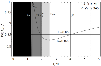
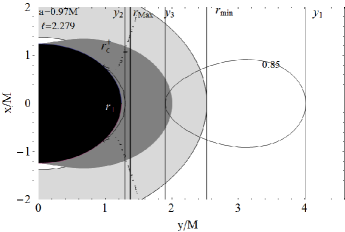
Figure 5: Left panel: logarithm plot of the effective potential $V_{eff}(\ell)$ as function of $r/M$. Right plot: the Boyer surface in the plane $(x,y)$ for a spacetime spin-mass ratio $a/M=0.97\in\mathbf{BHIX}$ and fluid angular momentum $\ell=2.279$ in units of mass $M$. Black regions are $r<r_{+}$ where $r_{+}$ is the black hole outer horizon, gray region is $]r_{+},r_{\epsilon}^{+}]$ where $r_{\epsilon}^{+}$ is the static limit, light-gray region is $]r_{\epsilon}^{+},r_{min}]$, the critical points of $V_{eff}(\ell)$ are signed in the plots: $r_{min}$ is a minimum point of $V_{eff}(\ell)$ and $r_{Max}$ a maximum point. The surfaces and the points at $K=V_{eff}(\ell)=$constant are black lines, the point $y_{1}$ (left plot) corresponds to the outer boundary of the disk section (right plot), $y_{3}$ to the inner one, and $y_{2}$ to the outer boundary of the innermost surface, $r_{min}$ sets the diks center.

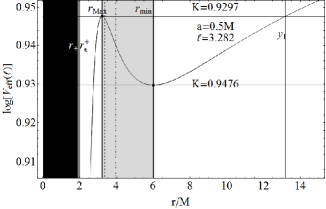
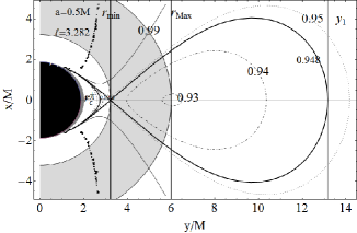
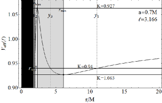
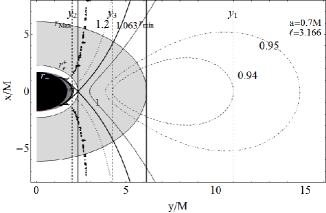
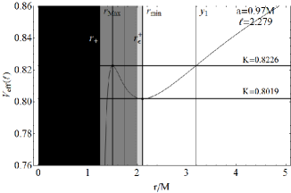
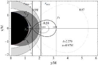
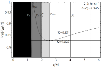
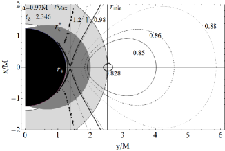
Figure 6: Left panels: logarithm plot of the effective potential $V_{eff}(\ell)$ as function of $r/M$. The angular momentum $\ell$ is in units of mass $M$. Right panels: the Boyer surface in the plane $(x,y)$ (sequences $\mathfrak{B}_{K}\equiv\mathfrak{B}_{\mathbf{p}}/\Sigma_{\ell}$ of P-D tori loops). Black regions are $r<r_{+}$ where $r_{+}$ is the outer black hole outer horizon, gray region is $]r_{+},r_{\epsilon}^{+}]$ where $r_{\epsilon}^{+}$ is the static limit, light-gray region is $]r_{\epsilon}^{+},r_{\min}]$, the critical points of $V_{eff}(\ell)$ are signed in the plots: $r_{min}$ is a minimum point of $V_{eff}(\ell)$ and $r_{Max}$ a maximum point. The surfaces and the points at $K=V_{eff}(\ell)=$constant are black lines, the point $y_{1}$ (left plot) corresponds to the outer boundary of the disk section, $y_{3}$ to the inner one, and $y_{2}$ to the outer boundary of the innermost surface, $r_{min}$ sets the disks center. First line for spacetime at $a=0.5M\in\mathbf{BHIII}$, second line for $a=0.7M\in\mathbf{BHV}$ and third and fourth lines $a=0.97M\in\mathbf{BHIX}$. Each contours in the right plots is at $K=$constant. It is $\ell=\ell_{f}^{+}(r_{Max})$, where $r_{Max}$ is the maximum point of the effective potential $K_{Max}$. The first and third row of plots is at $K_{Max}<1$. Fourth line is $K_{Max}=1$, second line $K_{Max}>1$. The radii $r:V_{eff}(a,\ell)=K$, within the critical points are shown in the plot of the effective potential.

Figures (5,6) show the Boyer surfaces crossing $r_{\epsilon}^{+}$ and eventually, the penetration of the disk surface in the region $r<r_{\epsilon}^{+}$. We consider the orbital region $\Delta_{crit}\equiv[r_{Max},r_{min}]$, whose boundaries correspond to the maximum and minimum points of the effective potential respectively (the minimum and maximum of the hydrostatic pressure). The innermost boundary of the P-D configuration, $y_{3}:\;y_{2}<y_{3}<y_{1}$, must be $y_{3}\in\Delta_{crit}$ the outer one is $y_{1}>r_{min}$, the center of the disk is located on $r_{min}$, the cross of the surfaces $C_{x}$ is at $r_{Max}$ and there are closed crossed surfaces if $K_{Max}<1$. Then at fixed $\ell$ the closed disk, as a point in $r_{min}$ (ring of particles at $p=0$), it grows (with $K$) to fill the entire region up to $r_{Max}$ where the accretion occurs: there are closed surfaces only if the constant parameter $K\in[K_{min},K_{Max}]$ where $K_{min}\equiv V_{eff}(\ell,r_{min})$ and $K_{Max}\equiv V_{eff}(\ell,r_{Max})$, light-gray regions of Figs. (5,6), such that there exist at last a solution at $K=V_{eff}(\ell,r)$ for the parameter couple $\mathbf{p}\equiv(K,\ell)$ fixed. A further matter configuration (with solution $y_{2}$) closest to the black hole is at $r<r_{max}$. However this scheme foreseen also areas in the space of $\mathbf{p}$-parameter, in BHIX spacetimes, entirely contained in the ergoregion i.e. $r_{min}<r_{\epsilon}^{+}$ and $r_{+}<y_{3}<r_{min}<y_{1}<r_{\epsilon}^{+}$, this implies the existence of at last a right neighborhood $I^{+}_{\mbox{\tiny{$r_{min}$}}}\subset\Sigma_{\epsilon}^{+}$ of the minimum radius (where $\Sigma_{\epsilon}^{+}\equiv]r_{+},r_{\epsilon}^{+}[$) with $\partial_{r}V_{eff}>0$ and $\partial_{r}^{2}V_{eff}>0$, or $y_{1}\in I^{+}_{\mbox{\tiny{$r_{min}$}}}:\;D(y_{1},y_{3})=0,\;D(y_{1},r_{min})>0$ where $D(r_{1},r_{2})\equiv V_{eff}(r_{1})-V_{eff}(r_{2})$. It can be shown that if $D(y_{1},r_{min})>0$ exists for some fixed $\mathbf{p}$, it remains small requiring a fine-tuning (on $10^{-3}$ for $K$). In the ergoregion the Killing vector $\xi_{t}^{a}$ becomes spacelike, but still the associated constant of motion (now it can be $E<0$) is well defined (see also discussion in Pugliese:2014ela ).

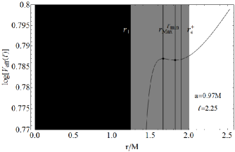
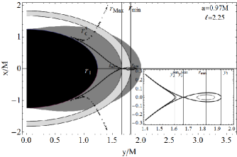
Figure 7: Left panel: effective potential $V_{eff}(\ell)$ versus the orbital radius $r/M$ at $a=0.97M$ (BHIX spacetime) and orbital fluid angular momentum $\ell=2.25$ in units of mass $M$. Right panel: Boyer surfaces at fixed $K$ (sequences $\mathfrak{B}_{K}\equiv\mathfrak{B}_{\mathbf{p}}/\Sigma_{\ell}$ of P-D tori loops). Black region is $r<r_{+}$ ($r_{+}$ being the outer horizon), the ergoregion (dark gray) is $r\in]r_{+},r_{\epsilon}^{+}[$ where $r_{\epsilon}^{+}$ is the static limit. The critical points of the effective potential are both in the ergoregion, the maximum, located in $r_{Max}=1.66346M$ and minimum $r_{min}=1.82079M$ are signed by thick black lines. Closed configuration are centered in $r_{min}$, the crossing points are at $r_{Max}$. In the right panel are configurations entirely contained in the ergoregion. Light gray region is the $[r_{Max},r_{min}]$ the contours of the Boyer surfaces associated to the $K_{Max}\equiv V_{eff}(r_{Max})=0.786937$ and $K_{min}\equiv V_{eff}(r_{min})=0.786588$ (crossed closed $C_{x}$) are in black thick lines. Inside panel, the surface at $K=0.7865\in]K_{mnin},K_{Max}[$ is closed and contained in the ergoregion. The surfaces boundaries $y_{1}=1.92614M$, $y^{Max}_{3}=1.66346M$ (configuration of maximum $K$) and $y^{min}_{2}=1.60392M$ (configuration of minimum $K$) are signed.

Fig. (7) shows the limiting case of a closed Boyer surface entirely contained in the ergoregion: both the critical points of the effective potential are included in $\Sigma_{\epsilon}^{+}$. A cross can occur for closed surfaces in the BHVI-IX spacetimes , that is where $r_{\gamma}^{-}<r_{\epsilon}^{+}$, since the inner boundary satisfies $y_{2}<r_{Max}<r_{\gamma}^{-}$ there could be funnels of matter crossing the static limit from the accretion point. The ergoregion is filled with “orbits” at $K=1$ only in the BHVII-III-IX spacetimes: $a\in]a_{\diamondsuit},M[$, $\ell=\ell_{b}^{-}$, $a_{\diamondsuit}\equiv 2\left(\sqrt{2}-1\right)M\approx 0.828427M$, and at $a_{\diamondsuit}$ it is $r_{b}^{-}=r_{\epsilon}^{+}$ where $\ell\approx 2.82843M$. And at $r\in]r_{+},r_{\epsilon}^{+}[$ it is $\ell/M\in]2,2\sqrt{2}[$ and $\bar{\ell}\in]2,2+\sqrt{2}[$. The critical points at $K\in]0,1[$ are both minima and maxima. For the minimum points inside the ergoregion the situation is as follows: for the BHIX attractors ( $a/M\in]a_{\natural},M]$) minima are in $r\in]r_{lsco}^{-},r_{\epsilon}^{+}[$, with angular momentum $\ell\in]\ell_{lsco}^{-},\ell_{f}^{-}(r_{\epsilon}^{+})[$. Configurations with $\bar{\ell}>1$ are inside the ergoregion in BHIX, and that is all the configuration inside the ergoregion are $\ell>a$. The maximum extension of normalized angular momentum in $r\in]r_{lsco}^{-},r_{\epsilon}^{+}[$ is $\bar{\ell}\in]2,5/2[$ but $\ell/M\in]2,(5\sqrt{2})/3[$. Inside the ergoregion saddle points are located in the BHIX spacetimes with $r_{lsco}^{-}$ with $\ell_{f}^{-}$, that is $\ell_{lsco}^{-}$ and $r_{f}^{\pm}(\ell_{lsco}^{-})$. A seddle point exist on the static limit at $a=a_{\natural}$ where $\ell={5\sqrt{2}}/{3}M$. In terms of the rationalized angular momentum it is $\bar{\ell}\in]2,5/2[$ and $\ell/M\in]2,(5\sqrt{2}/3[$. Maximum points in the ergoregion are located in $a\in]a_{\diamondsuit},a_{\natural}]$ with $\ell=\ell_{f}^{-}$, for BHIX sources maxima exist in the region $\in]r_{lsco}^{-},r_{\epsilon}^{+}[$. A maximum is located on the static limit for BHVII-VIII spacetimes where $a\in]a_{\diamondsuit},a_{\natural}[$ and $\ell=\ell_{f}^{-}(r_{\epsilon}^{+})$. Or maximum points, located on the orbits $r_{f}^{\pm}(\ell,a)$ are in the BHVII-VIII spacetimes with $\ell\in]\ell_{f}^{-}(r_{\epsilon}^{+}),\ell_{b}^{-}[$ and for the BHIX-class with $\ell\in]\ell_{lsco}^{-},\ell_{b}^{-}$. Then it is $\bar{\ell}\in]2,2+\sqrt{2}[$ and $\ell/M\in]{5\sqrt{2}}/{3},2\sqrt{2}[$. Configurations $K>1$ in the ergoregion are for $\bar{\ell}\in]2,5[$ and $\ell/M\in]2,{5}/{\sqrt{2}}[$. On the static limit we should consider the spacetime with $a_{\Box}\equiv 1/\sqrt{2}M$ where $r_{\gamma}^{-}=r_{\epsilon}^{+}$ with $\ell=\ell_{f}^{-}(r_{\epsilon}^{+})$. For BHVI spacetimes, characterized by $a\in]a_{\Box},a_{\diamond}[$, maxima are with $\ell\in]\ell_{f}^{-}(r_{\epsilon}^{+}),\ell_{\gamma}^{-}[$ in BHVI, then in BHVII-III with $\ell\in]\ell_{b}^{-},\ell_{\gamma}^{-}[$, while at $a=a_{\natural}$ with $\ell\in]\ell_{b}^{-},\ell_{f}^{-}(r_{\epsilon}^{+})[$, finally BHIX with $\ell\in]\ell_{b}^{-},\ell_{\gamma}^{-}[$. Further consideration on dynamics in this region can be found in Sec. (IV.4.4) where the matter configuration at $\ell=0$ ($L=0$) is considered.

IV.2 A sequence of torus shapes in evolution

In this section we explore the sequences $\mathfrak{B}_{\bar{\ell}}\equiv\mathfrak{B}_{\mathbf{p}}/\Sigma_{K}$ fixing $K\in]0,1[$, and considering different values of the rationalized angular momentum $\bar{\ell}\equiv\ell/a$, thus we distinguish the corotating fluids with $\bar{\ell}>1$ in Sec. (IV.2.1) and in Sec. (IV.2.2) the configurations $\bar{\ell}<1$, which include negative values for the fluid angular momentum or counterrotating configurations. The extreme case of “steady” fluid respect to the central object, in other words $\bar{\ell}=1$, or the counterrotating case $\bar{\ell}=-1$ will be considered in Sec. (III.4). Then it is convenient to introduce the angular momenta $\ell_{K}^{i}(a;K)\;i\in\{1,2,3\}$ such that $\ell_{K}^{i}:V_{eff}=K,\;\partial_{r}V_{eff}=0$. One can solve the first equation to get $\ell_{K}^{\pm}(a;r,K)$, the second equation gives the solutions $r_{i}$ as in Eq. (37) that is used in $\ell_{K}^{\pm}(a;r_{i},K)$ as in Eq. (14). It is $\ell_{K}^{\pm}(a;r_{i},K_{lsco}^{\pm})=\ell_{lsco}^{\pm}$ and $\ell_{K}^{\pm}(a;r_{i},K_{b}^{\pm})=\ell_{b}^{\pm}$.

IV.2.1 Fluid configurations at $\bar{\ell}>1$

We investigate the corotating configurations at $\bar{\ell}>1$, we consider the sequences $\mathfrak{B}^{>}_{\bar{\ell}}\equiv\left.\mathfrak{B}_{\mathbf{p}}\right|_{\bar{\ell}>1}/\Sigma_{K}$ the critical points for the hydrostatic pressure in this case are analysed in Sec. (III.4): three main regions,Region I–Region III, for the $K$ parameter can be recognized and different phases for the angular momentum parameter namely:

Region I:

$K\in]0,K_{lsco}^{-}]$; 1. $(\ell\in]a,\ell_{K}^{2}[,y_{123})$, 2. $(\ell_{K}^{2},y_{13})$, 3. $(\ell>\ell_{K}^{3},y_{1})$.

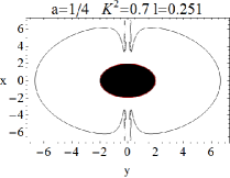
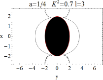
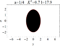
Figure 8: Configurations at $K<1$, $\ell>a$. Region $K\in]0,K_{lsco}^{-}]$. The spacetime spin is $a=0.25M\in\mathbf{BHI}$, the outer horizon is at $r_{+}=1.96825M$ the static limit $r_{\epsilon}^{+}=2M$, where $K^{2}=0.7$ (sequences $\mathfrak{B}_{\ell}\equiv\mathfrak{B}_{\mathbf{p}}/\Sigma_{K}$), it is $\ell_{{K}}^{i}=\{0.233022,0.270991\}$, and $\ell_{f}(r_{+})=15.746$, $\ell_{\epsilon}^{+}=13.4216$, $\ell_{f}(r_{d})=8.22857$, $\ell_{\gamma}^{-}=4.67535$, $\ell_{b}^{-}=3.73205$, $\ell_{lsco}^{-}=3.43993$, in units of mass $M$.

This region does not include closed (Boyer) surfaces or ${C}$-configurations, that is the effective potential has not minimum points. As shown in Figs. (8), the orbiting matter rotates around the attractor with a very clear evolution: increasing the angular momentum the configuration approaches the source, the torus becoming thinner (see also discussion in PuMonBe12 for the case $a=0$), the solutions around the rotation axis spread on the equatorial plane, we note also that at the axis of rotation there is a singularity due to the adopted frame. In some cases the surfaces cross the equatorial plane very close to the region $[r_{\epsilon}^{+},r_{+}]$. Then we introduce a new morphological type, fat torii, denoted as ${B}$-configurations, often with opened funnels, see also for a general discussion of the different torii Abramowicz:2011xu ; Raine ; BAF2006 ; Hawley1990 ; Abramowicz:2004vi . These surfaces could be associated to the innermost configurations surrounding the black hole, always present with the closed $C$ configurations and correspondent to the solution $y_{2}$ leading to the accretions at the instability point where $y_{2}=y_{3}$, matching the outer $C$ disk in a $C_{x}$ morphology.

Region II:

$K\in]K_{lsco}^{-},K_{lsco}^{+}[$: 1. $(\ell\in]a,\ell_{K}^{2}[,y_{123})$, 2. $(\ell=\ell_{K}^{2},y_{13})$, 3. $(\ell\in]\ell_{K}^{2},\ell_{K}^{3}[,y_{1})$, 4. $(\ell=\ell_{K}^{3},y_{13})$, 5. $(\ell\in]\ell_{K}^{3},\ell_{K}^{1}[,y_{23})$, 6. $(\ell=\ell_{K}^{1},y_{2})$, 7. $\ell>\ell_{K}^{1}$ see Fig. (9). In this case there are closed surfaces and ${B}$-configurations associated with lower angular momentum. With increasing angular momentum a pattern similar to Region I appears, starting with the ${C}_{x}$ configurations, it decreases in thickness, separates in the two Boyer lobes and then it disappears, leaving an open, not crossed configuration that is one could consider the sequence $\mathfrak{B}^{>}_{\bar{\ell}}=[B,{C}_{x},{C},{O}]$. In this region we considered both the limiting values $K_{lsco}^{\pm}$ even if we analyze the corotating matter only. The evolutive order in $\mathfrak{B}^{>}_{\bar{\ell}}$ should follow the decreasing angular momentum $\bar{\ell}$ to figure properly an accretion process onto the black hole, from $C$-topology to the $B$ one, starting from a former opened $O$ one.

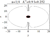
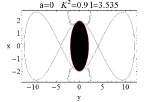
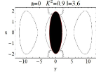
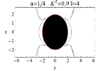
Figure 9: Configurations at $K<1$ and $\ell>a$. Region $K\in]K_{lsco}^{-},K_{lsco}^{+}[$. The spacetime spin is $a=0.25M\in\mathbf{BHI}$, the outer horizon is at $r_{+}=1.96825M$ the static limit $r_{\epsilon}^{+}=2M$, (sequences $\mathfrak{B}_{\ell}\equiv\mathfrak{B}_{\mathbf{p}}/\Sigma_{K}$) where $K^{2}=0.9$, it is $\ell_{K}^{i}=\{0.235225,0.268791,3.53586,3.69391\}$ and $\ell_{f}(r_{+})=15.746$, $\ell_{\epsilon}^{+}=13.4216$, $\ell_{f}(r_{d})=8.22857$, $\ell_{\gamma}^{-}=4.67535$, $\ell_{b}^{-}=3.73205$, $\ell_{lsco}^{-}=3.43993$. The fluid angular momentum is in units of mass $M$.

Region III

: $K\in[K_{lsco}^{+},1[$: 1. $(\ell\in]a,\ell_{K}^{1}[,y_{23})$, 2. $(\ell_{K}^{1},y_{3})$, 3. $(\ell\in]\ell_{K}^{4},\ell_{K}^{5}[,{y_{1}})$, 4. $(\ell_{K}^{5},y_{13})$, 5. $(\ell\in]\ell_{K}^{5},\ell_{K}^{6}[,{y_{123}})$, 6. $(\ell_{K}^{5},{y_{12}})$, 7. $(\ell>\ell_{K}^{6},{y_{1}})$. This is an articulated region. The surfaces approach the attractor increasing the angular momentum. Figs. (10) show a sequence of shapes analogue to Region II: with increasing orbital angular momentum the basic sequence of surfaces is: $\mathfrak{B}^{>}_{\bar{\ell}}=[{B},{C}_{x},{C},{O},{O}_{x},{O}]$. The last open configuration of $\mathfrak{B}^{>}_{\bar{\ell}}$ disappears into the black hole increasing $\ell>\ell_{k}^{6}$, . In this case the evolutive sequence $\mathfrak{B}^{>}_{\bar{\ell}}$ is quite articulated and to figure a disk evolution towards the accretion we should consider decreasing values of the rationalized angular momentum, neglecting then the starting sequence of opened configurations.

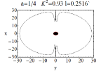
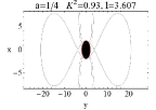
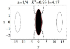
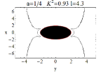
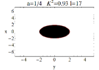
Figure 10: Configurations at $K<1$, $\ell>a$ in Region III $K\in[K_{lsco}^{+},1[$ (sequences $\mathfrak{B}_{\ell}\equiv\mathfrak{B}_{\mathbf{p}}/\Sigma_{K}$), see Sec. (IV.2.1). The spacetime spin is $a=0.25M\in\mathbf{BHI}$, the outer horizon is at $r_{+}=1.96825M$ the static limit $r_{\epsilon}^{+}=2M$, it is $K^{2}=0.93$ and $\ell_{K}^{i}\in\{-4.29142,-4.01885,0.235492,0.268524,3.60729,4.19897\}$, and $\ell_{f}(r_{+})^{\pm}=15.746$, $\ell_{\epsilon}^{+}=13.4216$, $\ell_{f}(r_{d})=8.22857$, $\ell_{\gamma}^{-}=4.67535$, $\ell_{lsco}^{-}=3.43993$, $\ell_{b}^{-}=3.73205$. and $\ell_{\gamma}^{+}=-5.68011$, $\ell_{b}^{+}=-4.23607$ $\ell_{lsco}^{+}=-3.88089$.

This analysis overlooks a small region of $K$-parameter very close to the zero that would require a fine-tuning of the configuration parameters. Figure (4)-left shows Region II and Region III on the plane $(K,a/M)$. A discussion on the maximum extension of the $K$-parameter has been addressed in Sec. (III.3.2).

IV.2.2 Fluid configuration at $\bar{\ell}<1$

In this section we focus on the corotating and counterrotating configurations at $\bar{\ell}<1$ and the sequence $\mathfrak{B}^{<}_{\bar{\ell}}\equiv\left.\mathfrak{B}_{\mathbf{p}}\right|_{\bar{\ell}<1}/\Sigma_{K}$ : the situation is much more detailed as we approach the limits $\bar{\ell}\lessapprox 0$ and $\bar{\ell}\gtrapprox 0$. In this case we can identify three regions for the $K$-parameter and different phases for the evolution of the $\ell$-parameter. As shown in Sec. (III.4), the critical points for the pressure can be only at $\bar{\ell}<-1$, therefore only counterrotating P-D configurations are allowed with $\bar{\ell}<1$. The only limiting value for the $K$-parameter is $K_{lsco}^{+}(a)=V_{eff}(a;\ell_{lsco}^{+})$ associated to counterrotating orbits only.

Region I:

$K\in]0,K_{lsco}^{+}[$; 1. $(\ell<\ell_{K}^{1}\,{y_{1}})$ 2. $(\ell_{K}^{1},y_{13})$, 3. $(\ell\in]\ell_{K}^{1},a[\;{y_{123}})$. This case is illustrated in Fig. (11). There are both corotating and counterrotating ${B}$-configurations: decreasing the magnitude of the orbital angular momentum the configuration stretches along the axis on the equatorial plane. In Tables. (13) it is show the set of counterrotating and corotating fluids respect a change in $K$ and $\ell$. We note that the boundary of this region is determined by $K_{lsco}^{+}$ only for both $\ell>0$ and $\ell<0$, however only counterrotating configurations at $\bar{\ell}<1$ can give rise to P-D tori, as discussed in Sec. (III.3.2) and Sec. (III.4).

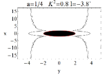
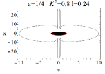
Figure 11: Configurations at $K<1$, $\ell<a$ in Region I $K\in]0,K_{lsco}^{+}[$ see Sec. (IV.2.2). The spacetime spin is $a=0.25M\in\mathbf{BHI}$, (sequences $\mathfrak{B}_{\ell}\equiv\mathfrak{B}_{\mathbf{p}}/\Sigma_{K}$) where $K=0.81$, the outer horizon is at $r_{+}=1.96825M$ the static limit $r_{\epsilon}^{+}=2M$, $\ell_{K}^{i}=\{0.234227,0.269787\}$, in units of mass $M$.

Region II:

$K_{lsco}^{+}$: 1. $(\ell<\ell_{K}^{3},{y_{1}})$, 2. $(\ell_{K}^{3}\;y_{13})$, 3. ($\ell\in]\ell_{K}^{3},a[\;{y_{123}})$. This is a limiting case and, accordingly to the analysis in Fig. (4) it corresponds to an unstable orbit located in $r_{lsco}^{+}$.

Region III:

$K\in]K_{lsco}^{+},1[$, 1. $(\ell<\ell_{K}^{1}\;{y_{1}})$ 2. $(\ell_{K}^{1}\;{y_{12}})$, 3. $(\ell\in]\ell_{K}^{1},\ell_{K}^{2}[\;{y_{123}})$ 4. $(\ell_{K}^{2},{y_{13}})$ 5. $(\ell\in]\ell_{K}^{2},\ell_{K}^{3}[{y_{1}})$ 6. $(\ell_{K}^{3}\;{y_{12}})$ 7. $(\ell\in]\ell_{K}^{3},a[\;{y_{123}})$. This case is illustrated in Figs. (12) and it includes the Boyer surfaces: decreasing the angular momentum magnitude up to zero there are ${B}$ configurations then a closed ${C}$ configuration appears, and only after this stage, in contrast with the corotating case in Region III of Sec. (IV.2.1), a closed-crossed ${C}_{x}$ surface appears, it is then followed by a second ${B}$-configuration with matter aligned to the axes. With increasing angular momentum the fluid stretches on the equatorial plane and finally tends to thicken up to the ${B}$-configuration, with thickness close to the unity, then one can say the set of surfaces is $\mathfrak{B}^{<}_{\bar{\ell}}=[B,C,C_{x},B]$.

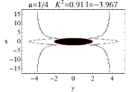
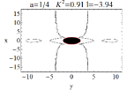
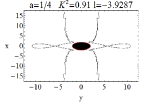
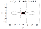
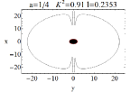
Figure 12: Configurations at $K<1$, $\ell<a$. in Region III $K\in]K^{+}_{lsco},1[$ see Sec. (IV.2.2). The spacetime spin is $a=0.25M\in\mathbf{BHI}$, the outer horizon is at $r_{+}=1.96825M$ the static limit $r_{\epsilon}^{+}=2M$, (sequences $\mathfrak{B}_{\ell}\equiv\mathfrak{B}_{\mathbf{p}}/\Sigma_{K}$) where $K^{2}=0.91$, it is $\ell_{K}^{i}=({-3.96369},{-3.92872},{0.235316},{0.2687},{3.56152},{3.82688})$. The angular momentum is in units of mass $M$.

IV.3 The model evolution for different $K$ at $\ell$ fixed

Here we analyse the sequence $\mathfrak{B}_{K}\equiv\mathfrak{B}_{\mathbf{p}}/\Sigma_{\ell}$. It is convenient to address the discussion separating the two subcases of the corotating $\ell>0$ configurations in Sec. (IV.3.1) and counterrotating $\ell<0$ configurations in Sec. (IV.3.2). In Sec. (IV.3.3) we explore the open configuration $K>1$.

IV.3.1 Corotating $(a\ell>0)$ fluid configurations at $K<1$

We focus on the corotating orbits $\ell>0$ at $K<1$. The situation is very articulated, it is shown schematically in Table (13)-right and discussed in six macroregions, defined by fixed $\ell$ and varying the $K$-parameter, each region of angular momentum values include different subregions for the variation of the $K$-parameter.

Region I

We consider three sub regions of $\ell$-parameters namely: $\mathbf{Ia}$ for $\ell\in]0,\ell_{\mu}^{\Pi}[$: 1. $(0,y_{23})$, 2. $(K\in]0,K_{2}[,y_{123})$. 3. $(K_{2},y_{13})$, 4. $(K\in]K_{2},1[,y_{1})$. $\mathbf{Ib}$ for $\ell\in[\ell_{\mu}^{\Pi},a[$: 1. $(0\,y_{23})$, 2. $(K\in]0,1[,y_{123})$. $\mathbf{Ic}$ for $\ell=a$: 1. $(K\in[0,1[,y_{23})$. This region corresponds to $\bar{\ell}<a$ for corotating matter plotted in Figs. (11, 12) and detailed in Sec. (IV.2.2), the last subregion $\ell=a$, is a limiting case and it will be investigated further in Sec. (IV.4.3). As discussed in Sec. (III.4) there are no P-D tori but in general $B$-surfaces can be formed, there is one solution of the equation $\mathcal{V}_{eff}=0$ corresponding to the exterior boundary of the disk. The boundary $\ell_{\mu}^{\Pi}<a$ is defined and discussed in Eq. (38) and illustrated in Fig. (2).

Region II

This case can be analysed in four ranges of variation of $\ell$. $\mathbf{IIa}$ for $\ell\in]a,\ell_{f}^{\pm}(r_{-})[$ it is 1. $(0,y_{23})$, 2. $(K\in]0,1[,y_{123})$, $\mathbf{IIb}$ for $\ell=\ell_{f}^{\pm}(r_{-})$ it is 1. $(0,y=3)$, 2. $(K\in]0,1[,y_{23})$. $\mathbf{IIc}$ for $\ell\in]\ell_{f}^{\pm}(r_{-}),-\ell^{\Pi}_{\mu}]$ it is 1. $(0,y_{23})$, 2. $(K\in]0,1[,y_{123})$. $\mathbf{IId}$ for $\ell\in]-\ell^{\Pi}_{\mu},\ell_{lsco}^{-}]$ it is 1. $(0,y_{23})$, 2. $(K\in]0,K_{2}[,y_{123})$, 3. $(K_{2},y_{13})$, 4. $(K\in]K_{2},1[,y_{1})$. The location of the angular momenta as function of $a/M$ is illustrated in Fig. (2) however it is $\ell_{f}^{\pm}(r_{-})<\ell_{lsco}^{-}$. No closed Boyer surfaces are possible.

Region III

. The configurations are as follows: $\mathbf{IIIa}$ for $\ell\in]\ell_{lsco}^{-},\ell_{b}^{-}[$ it is then 1. $(0,y_{23})$, 2. $(K\in]0,K_{2}[,y_{123})$, 3. $(K_{2},y_{13})$, 4.$(K\in]K_{2},K_{1}[\cup K_{3},y_{13})$, 5. $(K\in]K_{3},K_{4}[,y_{123})$, 6. $(K_{4},y_{13})$, 7. $(K\in]K_{4},1[,y_{1})$. This region of fluid angular momentum allows the formation of P-D configurations, see also Fig. (4) the corresponding class for in terms of the rationalized angular momentum is Region II and Region III in Sec. (IV.2.1). The maximum of the effective potential with $K<1$is associated to the closed crossed ${C}_{x}$ surfaces, when $\ell\in]\ell_{lsco}^{-},\ell_{b}^{-}[$, as described in Sec. (III.3) and Eq. (2).

Region IV

There is only one set of values for the fluid angular momentum to be considered. $\mathbf{IVa}$ for $\ell\in[\ell_{b}^{-},\ell_{\gamma}^{-}]$ it is 1. $(0,y_{23})$, 2. $(K\in]0,K_{2}[,y_{123})$, 3. $(K_{2},y_{13})$, 4. $K\in]K_{2},K_{3}],y_{1})$, 5.$(K_{3},y_{12})$, 6. $(K\in]K_{3},1[,y_{123})$. When $K>1$ there are maximum points only i.e. ${O}_{x}$-configurations at $r=r_{f}^{\pm}$ for $]\ell_{b}^{-},\ell_{\gamma}^{-}$; for $K\in]K_{lsco}^{\pm},1[$ the minimum points, ${C}$ are for $\ell>\ell_{lsco}^{-}>0$ and $r>r_{lsco}^{\pm}$, see Table (13)-right.

Region V

We distinguish two ranges of angular momentum. $\mathbf{Va}$: for $\ell\in]\ell_{\gamma}^{-},\ell_{f}^{\pm}(r_{+})[$ the situation is as follows 1. $(0,y_{23})$, 2. $(K\in]0,K_{2}[,,y_{123})$, 3. $(K_{2},y_{13})$, 4. $(K\in]K_{2},K_{4}[,y_{3})$, 5. $(K_{4},y_{12})$, 6. $(K\in]K_{4},1[,y_{123})$, $\mathbf{Vb}$ for $\ell=\ell_{f}^{\pm}(r_{+})$: 1.$(0,y_{2})$, 2. $(K\in]0,K_{3}[,y_{123})$, 3. $(K_{3},y_{1})$, 4. $(K_{4},y_{2})$, 5. $(K\in]K_{4},1[,y_{123})$,

Region VI

We consider the following set $\mathbf{VIa}$ for $\ell>\ell_{f}^{\pm}(r_{+})$ it is 1.$(0,y_{23})$, 2.$(K\in]0,K_{3}[,y_{123})$, 3.$(K_{3},y_{12})$, 4. $(K\in]K_{3},K_{4}[,y_{1})$, 5. $(K_{4},y_{12})$, 6. $(K\in]K_{4},1[,y_{123})$ see also Fig. (4).

The union of Region III-VI corresponds to $\ell>\ell_{lsco}^{-}$. Table (13)-right summarizes this situation.

IV.3.2 Counterrotating $(a\ell<0)$ fluid configurations at $K<1$

We focus on the case $\ell<0$ (counterrotating fluid configurations). We summarize the situation in Table (13). This case $a\ell<0$ is much less articulated then for the corotating fluids and here we can distinguish four regions of angular momentum:

Region I

for $\ell<\ell_{\gamma}^{+}$: 1. $(K\in]0,K_{1}[,{y_{23}})$, 2. $(K_{1},y_{13})$, 3. $(K\in]K_{3},K_{4}[,{y_{1}})$, 4. $(K_{4},{y_{12}})$, 5. $(K\in]K_{4},1[,y_{123})$. For angular momentum in this range there are no critical points for the effective potential and no Boyer surfaces.

Region II

for $\ell\in[\ell_{\gamma}^{+},\ell_{b}^{+}]$: 1. $(K\in]0,K_{2}[,y_{123})$, 2. $(K_{2},y_{13})$, 3. $(K\in]K_{2},K_{3}[,y_{1})$, 4. $(K_{3},y_{12})$, 5. $(K\in]K_{3},1[,y_{123})$. The effective potential admits critical unstable and unbounded orbits, Fig. (4). There are only open $O_{x}$ surfaces.

Region III

for $\ell\in]\ell_{b}^{+},\ell_{lsco}^{+}[$: 1. $(K\in]0,K_{2}[,y_{123})$, 2. $(K_{2},y_{13})$, 3. $(K\in]K_{2},K_{3}[,y_{1})$, 4. $(K_{3},y_{12})$, 5. $(K\in]K_{3},K_{4}[,y_{123})$, 6. $(K_{4},y_{13})$, 7. $(K_{4}\in]K_{4},1[y_{1})$. Critical points are in the Regions I-II-III, there are only closed or closed crossed surfaces: closed crossed ${C}_{x}$ surfaces, where $\ell\in]\ell_{b}^{+},\ell_{lsco}^{+}[$ while $C$ configurations are for $\ell<\ell_{lsco}^{+}<0$, as $K\in]K_{lsco}^{\pm},1[$.

Region IV

for $\ell\geq\ell_{lsco}^{+}$: 1. $(K\in]0,K_{2}[,y_{123})$, 2. $(K_{2}\,y_{13})$, 3. $(K\in]K_{2},1[,y_{1})$. There are no closed $C$-configurations see Table (13) and Figs. (4).

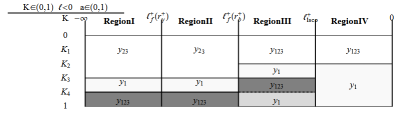
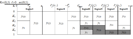
Figure 13: Configurations of the fluid angular momentum $\ell=\ell(a)<0$, left panel, and $\ell=\ell(a)>0$ right panel. Existence regions of the zeros $y_{i}$ of $\mathcal{V}_{eff}(\mathbf{p})\equiv V_{eff}(\ell)-K$ for fixed ranges of angular momentum, and the potential-parameter $K_{i}=K_{i}(a,\ell)\in]0,1[$. In the dark gray-shaded regions closed $C$ Boyer disks exist.

Tables (13) together show the maximum and minimum extension of the $\mathbf{p}$ parameter for the existence of a P-D configuration, it is clear the gap for $\ell\in]\ell_{lsco}^{+},\ell_{lsco}^{-}[$, where no P-D configurations are possible, and the presence of the limiting values $K_{4}$ and $K_{3}$, for the set of $K$-parameter. It is important to note that this analysis does not take into account the attractor spin explicitly but through the angular momentum $\ell^{i}_{K}(a;K)$ or the parameter $K_{i}(a;\ell)$. Moreover, there is no evidence of a clear evolutive set $\mathfrak{B}_{K}$ for both the $a\ell<0$ or $a\ell>0$ cases. This would confirm that a better choice for a dynamical parameter could be the fluid angular momentum $\ell$ or $\bar{\ell}$. However we will address more deeply this point in Sec. (IV.4.1) where, considering a non rotating attractor, we detail the possible $\mathfrak{B}_{K}$ sequences and we give also some general considerations comparing the $\mathfrak{B}_{K}$ and $\mathfrak{B}_{\ell}$ sequences.

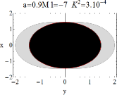
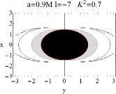
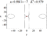
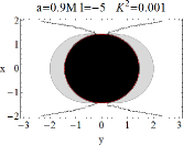
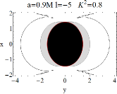
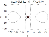
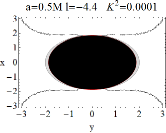
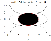
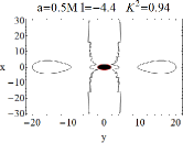
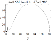
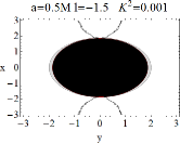
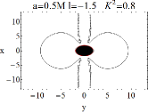
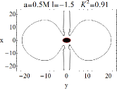
Figure 14: Closed Boyer surfaces (sequences $\mathfrak{B}_{K}\equiv\mathfrak{B}_{\mathbf{p}}/\Sigma_{\ell}$) for fixed ranges of the fluid angular momentum $\ell=\ell(a)<0$ in units of mass $M$ and the potential-parameter $K_{i}=K_{i}(a,\ell)\in]0,1[$ in different spacetimes. It is: $a=9/10M\in\mathbf{BHVIII}$ and $\ell_{\gamma}^{+}=-6.83232$ and $(K_{i})^{2}\in\{0.977871,0.000828153\}$ Second row: $\ell_{f}^{+}(r_{b}^{+})=-4.75681$ and $(K_{i})^{2}\in\{0.00146791,0.951018\}$. Third row: $a/M=5/10\in\mathbf{BHIII}$, $\ell_{f}^{+}(r_{b}^{+})=-4.44949$ and $\ell_{f}^{+}(r_{lsco}^{+})=-4.06784$ $(K_{i})^{2}\in\{0.000172721,0.932708,0.984353\}$, Bottom row: $a/M=5/10\in\mathbf{BHIII}$, $(K_{i})^{2}\in\{0.00102636,0.900794\}$

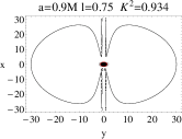
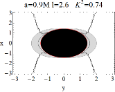
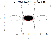
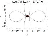
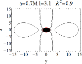
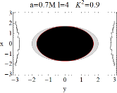
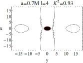
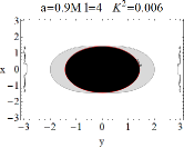
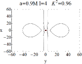
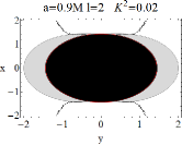
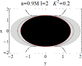
Figure 15: Closed Boyer configurations for fixed ranges of the fluid angular momentum $\ell=\ell(a)>0$ in units of mass $M$ and the parameter $K_{i}=K_{i}(a,\ell)\in]0,1[$ for spacetime $a=9/10M\in\mathbf{BHVIII}$ and $a=7/10M\in\mathbf{BHV}$.

IV.3.3 The evolution of the models for $K>1$ at $\ell$ fixed

In this section we consider the the sequences $\mathfrak{B}_{K}\equiv\mathfrak{B}_{\mathbf{p}}/\Sigma_{\ell}$ for $K>1$. There are no closed configurations, and in general critical points are in $r\in]r_{\gamma}^{\pm},r_{b}^{\pm}[$ for corotating and counterrotating matter respectively, see Sec. (III.3.3). At $K>1$ only maximum of the effective potential, or minimum of the pressure, are possible. These surfaces, however, could shape jets crossing the equatorial plane in one or more points.

Corotanting fluids ($\ell>0$)

Region I

for $\ell\in]-\ell_{\mu}^{\Pi},a[$ it is: 1. $(K\in]1,K_{2}[,y_{23})$, or 2. $(K=K_{2},{y_{2}})$ and for $\ell=a$: ir is $(K>1,y_{3})$. This region corresponds to the solutions with $\bar{\ell}<1$, where critical points cannot exist.

Region II

For $\ell\in]a,\ell_{f}^{\pm}(r_{-})[$ it is $(K>1,y_{23})$. For the particular values $\ell=\ell_{f}^{\pm}(r_{-}):$ it is $(K>1,y_{2})$. In the range $\ell\in]\ell_{f}^{\pm}(r_{-}),\ell_{a}^{1}]:\quad(K>1,y_{23})$, and finally for $\ell\in]\ell_{a}^{1},-\ell^{\Pi}_{\mu}[$ it is , $\mathbf{1.}\quad(K\in]1,K_{2}[,y_{23}),\mathbf{2.}\quad(K_{2},{y_{2}})$. A limit case for configurations of Region II is the non rotating background of the Schwarzschild geometry, some configurations at $a=0$ are for example in Fig. (20). However the introduction of a spin for the attractor does not change qualitatively this structure for the Region II.

Region III

For fluids with $\ell\in]\ell_{b}^{-},\ell_{\gamma}^{-}[$, solutions are for $\mathbf{1.}\quad(K\in]1,K_{4}[\;y_{23})$, and $\mathbf{2.}\quad(K_{4},{y_{2}})$. In this region P-D configurations of the type $O_{x}$ are possible, see also Fig. (4).

Region IV

For corotating fluids with $\ell\in[\ell_{\gamma}^{-},\ell_{f}^{\pm}(r_{+})[$, it is 1. $(K>1,y_{23})$, while in the limit case $\ell_{f}^{\pm}(r_{+})$, it is $(K>1,y_{3})$.

Region V

In this region we consider only fluid configurations with $\ell>\ell_{f}^{\pm}(r_{+})$, where solutions are for $(K>1,y_{23})$.

Counterrotating fluids $\ell<0$ Here we focus on the case of counterrotating fluids and the sequences $\mathfrak{B}_{K}$, two regions of values of $\ell$ need to be considered (see also $\mathfrak{B}_{\bar{\ell}}$ sequences considered in Sec. (IV.2.2)).

Region I:

$\ell\leq\ell_{\gamma}^{+}$, 1. $(K>1,y_{23})$

Region II:

$\ell\in]\ell_{\gamma}^{+},\ell_{b}^{+}[$: 1. $(K\in]1,K_{4}[,y_{23})$ 2. $(K_{4},y_{2})$. In this region open crossed, $O_{x}$ are possible.

The case $a\neq 0$ is not qualitatively different from the situation for a Schwarzschild attractor, however a careful analysis should take into account the greater or lesser collimation of the open surfaces with respect to the rationalized angular momentum $\bar{\ell}$, and in an extended P-D model in GRMHD the influence of the magnetic field for the corotating and counterrotating configurations should be taken into account as well, for open solutions could play an important role in the jets analysis even where there is also a magnetic contribution Meier ; Abramowicz:2011xu .

IV.4 Some general considerations on the limiting cases

IV.4.1 Fluid configurations in the Schwarzschild spacetime

We focus now on the case of non rotating attractors. The P-D models in the Schwarzschild spacetime have been extensively analyzed for example in PuMonBe12 , here we reproduce the analysis in Sec. (IV.3) for the limiting case $a=0$. It is convenient to introduce the angular momentum $\ell_{\mathfrak{K}}^{\pm}(K)$

$$\frac{\ell_{\mathfrak{K}}^{\pm}}{M}\equiv\frac{\sqrt{27+\frac{1}{1-K^{2}}-\frac{8}{K^{2}}\pm\sqrt{\frac{(9K^{2}-8)^{3}}{(K^{2}-1)^{2}K^{2}}}}}{\sqrt{2}}$$ (39)

and the ${K}_{i}(\ell)$ functions or

$${K}_{a}\equiv\sqrt{\frac{\ell^{2}-36M^{2}-2\beta_{1}\sin\left(\frac{1}{3}\arcsin\alpha_{1}\right)}{3\ell^{2}-81M^{2}}},\quad{K}_{b}\equiv\sqrt{\frac{\ell^{2}-36M^{2}+2\beta_{1}\cos\left(\frac{1}{3}\arccos\alpha_{1}\right)}{3\ell^{2}-81M^{2}}},$$ (40)

and $K_{a}>K_{b}$ in $\ell>3\sqrt{3/2}M$ and $K_{a}=K_{b}$ in $\ell=3\sqrt{3/2}M$ with

$$\alpha_{1} \equiv \frac{\left(3^{9}\,8\right)M^{8}-\left(108\sqrt{2}\right)^{2}\ell^{2}M^{6}+\left(6\sqrt{51}\right)^{2}{\ell^{4}}M^{4}-72{\ell^{6}}M^{2}+{\ell^{8}}}{\ell^{2}\beta_{1}^{3}},\quad\beta_{1}\equiv(\ell^{2}-27M^{2})\sqrt{\frac{72M^{4}+(\ell^{2}-24M^{2})^{2}}{(\ell^{2}-27M^{2})^{2}}},$$ (41)

introduced and studied in PuMonBe12 they are special cases of $\ell_{K}^{i}(a,K)$ and $K_{i}(a,\ell)$ for $a=0$. As it is $a=0$ there is no need to distinguish between corotating and counterrotating fluid matter and we can summarize this special case as follows:

Fixed orbital angular momentum $\ell$ We consider the range $K\in]0,1[$ and the evolutive sequences $\mathfrak{B}_{K}\equiv\mathfrak{B}_{\mathbf{p}}/\Sigma_{\ell}$ thus we can compare this case with the analysis in Sec. (IV.3.1) it is then:

For $\ell/M\in]0,3\sqrt{{3}/{2}}]$ solutions are for $(K\in]0,1[,y_{1})$, Fig. (17).

For $\ell/M\in]3\sqrt{{3}/{2}},4[$: it is for 1. $(K\in]0,K_{b}[,{y_{1}})$, and 2. $({K_{b}},{y_{12}})$, or 3. $(K\in]K_{b},K_{a}[,y_{123})$ and 4. $(K_{a},y_{13}$. Finally 5. $(K\in]K_{a},1[,{y_{1}})$.

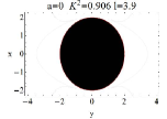
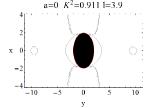
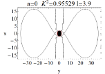
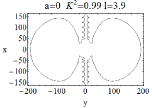
Figure 16: The Schwarzschild case: sequence $\mathcal{B}_{K}$ in $\ell/M\in]3\sqrt{{3}/{2}},4[$. It is $\ell=3.9M$ in units of mass $M$ and $K^{2}_{i}=\{0.95529,0.910634\}\quad i\in\{a,b\}$. The angular momentum is in units of mass $M$.

See Figs. (16). At fixed $\ell$ as $K$ increases the ${B}$-configurations will form a nucleus of Boyer thin disk quite far from the black hole increasing then in thickness and reconciling to the accretion configuration, to recreate again the configuration ${B}$ i.e. one could consider the sequence $\mathfrak{B}_{K}=[{B},{C},{C}_{x},{B}]$.

For $\ell\in[4,3\sqrt{3}]$: 1. $(K\in]0,{K_{b}}[,{y_{1}})$, 2. $(K_{b},y_{12})$, 3. $(K\in]K_{b},1[,{y_{123}})$. See Figs. (17). In this case as in the previous region it is $\mathfrak{B}_{K}=[{O},{B},{C}]$ and the surfaces along the axis stretch on the equatorial plane.

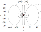
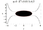
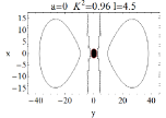
Figure 17: The Schwarzschild case sequence $\mathcal{B}_{K}$. Left panel:$\ell/M\in]0,3\sqrt{{3}/{2}}]$ with $(K\in]0,1[,y_{1})$. Center and right panel: $\ell/M\in[4,3\sqrt{3}]$, it is $\ell=4.5M$ and $K^{2}_{i}=\{1.47765,0.939964\}\quad i\in\{a,b\}$. The angular momentum is in units of mass $M$.

For $\ell/M>3\sqrt{3}$: 1. $(K\in]0,K_{b}[,{y_{1}})$, 2. $({K_{b}},{y_{12}})$, 3. $(K\in]K_{b},1[,{y_{123}})$

Fixed orbital parameter $K$ We will consider the range $K>0$ and the evolutive sequences $\mathfrak{B}_{\ell}\equiv\mathfrak{B}_{\mathbf{p}}/\Sigma_{K}$. We can compare this case with the analysis in Sec. (IV.2.1) and Sec.  (IV.2.2) it is then:

${K\in]0,\sqrt{{8}/{9}}]}$

there are the solutions $(\ell=0,y=3M)$ and $(\ell>0,y=M)$, see Figs. (18). The limiting case $\ell=0$ is shown here, with increasing $\ell$ a ${B}$-configuration emerges.

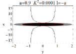
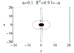
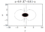
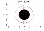
Figure 18: Configurations $\ell=\pm a$ and different spin-mass ratio of the attractors. The angular momentum is in units of mass $M$.

$K\in]\sqrt{{8}/{9}},1[$

there are the following solutions for increasing angular momentum: 1. $(\ell=0,y=3M)$, 2. $(\ell\in]0,\ell_{\mathfrak{K}}^{-}[,y=M)$, 3. $(\ell_{\mathfrak{K}}^{-},y_{13})$, 4. $(\ell\in]\ell_{\mathfrak{K}}^{-},\ell_{\mathfrak{K}}^{+}[,y_{123})$, 5. $(\ell_{\mathfrak{K}}^{+},y_{12})$, 6. $(\ell>\ell_{\mathfrak{K}}^{+},y=M)$. See Figs. (19): increasing $\ell$ the configurations sequence becomes $\mathfrak{B}_{\ell}=[{B},{C}_{x},{C}]$, closed surfaces finally disappear and only the interior ${B}$-surface, close to the black hole with open funnels of matter aligned with the axis.

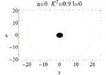
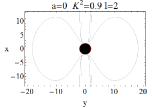
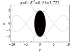
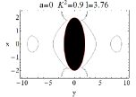
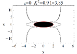
Figure 19: Non rotating attractor: sequences $\mathbf{B}_{\ell}$ with fixed $K\in]\sqrt{{8}/{9}},1[$. The angular momentum is in units of mass $M$. It is $K^{2}=0.9$ and $\ell_{\mathfrak{K}}^{\pm}\in\{3.72678,3.77124\}$.

$K=1$:

1. $(\ell<-4M,y_{12})$, 2. $(\ell=-4M,,y=4M)$, 3. $(\ell=4M,y=4M)$, 4. $(\ell>4M,y_{12})$, see Figs. (20-left). These are open configurations, these solutions could simulate jets.

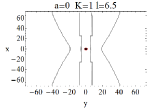
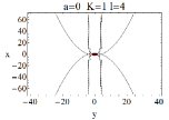
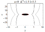
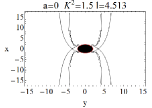
Figure 20: Non rotating attractor, sequences $\mathcal{B}_{\ell}$ for $K=1$ and $K>1$ where $K^{2}=1.5$ and $\ell_{\mathfrak{K}}^{+}=4.51276M$.

$K>1$:

1. $(\ell_{\mathfrak{K}}^{+},y=2M)$, 2. $(\ell>\ell_{\mathfrak{K}}^{+},y_{23})$. See Figs. (20) there are only open configurations.

In the limiting case of the Schwarzschild geometry we compare the two evolutive sequences $\mathfrak{B}_{\ell}$ and $\mathfrak{B}_{K}$, tracing out some general considerations for the case $a\neq 0$. The first sequence $\mathfrak{B}_{\ell}$ has been addressed extensively for the rotating case in Sec. (IV.2) and $\mathfrak{B}_{K}$ has been considered in Sec. (IV.3), however we restrict our attention to the case the only sequences including the Boyer closed or closed crossed configurations. Typical patterns are $\mathfrak{B}^{>}_{\bar{\ell}}=[B,{C}_{x},{C},{O}]$ as seen in Region II-Sec. (IV.2.1), and $\mathfrak{B}^{<}_{\bar{\ell}}=[B,C,C_{x},B]$ in Region III of Sec. (IV.2.2), finally it is $\mathfrak{B}_{K}=[{B},{C},{C}_{x},{B}]$, analyzed for the case of a Schwarzschild attractor. We note a symmetry in the sequences $\mathfrak{B}^{>}_{\bar{\ell}}$ and $\mathfrak{B}^{<}_{\bar{\ell}}$ with respect to the corotating and counterrotating fluids and the configurations $(C,C_{x})$ , clear also by the Tables (13), actually the two sequences appear to be analogue once one considers the increasing values of the fluid angular momentum magnitude, irrespectively from the cases $\ell a>0$ or $\ell a<0$: the evolutive sequence $(C,C_{x})$ appears decreasing the fluid angular momentum magnitude or increasing, at fixed $\ell$, the $K$-parameter, see the $\mathfrak{B}_{K}$ sequence, this kind of symmetries will be also investigated in Sec. (IV.5) and Sec. (IV.6) addressing the analysis of the Boyer surfaces structures and the disk morphology.

IV.4.2 Configuration at $K=1$

The case $K=1$ has been analyzed in Sec. (III.3.1), critical points are maximum of the effective potential and are located at $r_{b}^{\pm}$ with $\ell_{f}^{\pm}$ respectively. In other words we consider the special sequences $\mathfrak{B}_{\ell}\equiv\mathfrak{B}_{\mathbf{p}}/\left.\Sigma_{K}\right|_{K=1}$. This case completes the analysis of Sec. (IV.2) and Sec. (IV.3) and can be compared with the results in Sec. (IV.2). However we introduce the solutions

$$y_{\pm}\equiv\frac{1}{4M}\left(\ell^{2}\pm\sqrt{[\ell^{4}-16M^{2}(-\Delta_{\ell}^{-})^{2}]}\right),$$ (42)

limiting cases of the solutions $y_{i}$ in Eqs. (37) for $K=1$. Solutions (42) depend on the magnitude $|\ell-a|$ and it is $\ell_{K}^{\pm}(a;r_{i},K_{b}^{\pm})=\ell_{b}^{\pm}\equiv\ell_{f}^{\pm}({r_{b}^{\pm}})$. We summarize the results as follows:

The Schwarzschild case $a=0$:

There are only two regions as follows: Region I where 1. $(\ell<-4M,\;y_{\pm})$, 2. $(\mp 4M,\;y=4M)$, and Region II with solution $(\ell>4M,\;y_{\pm})$.

Kerr spacetime:

$a\in]0,1[$: Region I: 1. $(\ell<\ell_{b}^{+},y_{\pm})$, 2.$((\ell_{b}^{+},\ell_{\mu}^{\Pi}),y_{-})$, 3. $(\ell\in]\ell_{\mu}^{\Pi},a[,y_{\pm})$, 4. $(\ell=a\ y_{+})$. This first region consider the values $\bar{\ell}\in[0,1]$, for counterrotating fluids ($\ell a<0$) and corotating ones ($\ell a>0$) where no critical points are, and the values $|\bar{\ell}|>1$ at $\ell a<0$ where there is a maximum for the effective potential at $K=1$, see also Sec. (IV.2.2). Region II: In this region it is $\bar{\ell}>1$ and it includes various subregions: 5. $(\ell\in]a,\ell_{f}^{\pm}(r_{-})[,y_{\pm})$, 6. $(\ell_{f}^{\pm}(r_{-}),y_{-})$, 7. $(\ell\in]\ell_{f}^{\pm}(r_{-}),\ell^{\Pi}_{\mu}[,y_{\pm})$, 8. $(-\ell^{\Pi}_{\mu},y_{-})$, 9. $({\ell}_{b}^{-},y_{-})$, 10. $(\ell\in({\ell}_{b}^{-},\ell_{f}^{\pm}(r_{+})),y_{\pm})$, 11. $(\ell_{f}^{\pm}(r_{+}),y_{+})$, 12. $(\ell>\ell_{f}^{\pm}(r_{+}),y_{\pm})$. This region considerers $\bar{\ell}>1$ analysed for $K\neq 0$ in Sec. (IV.2.1).

Extreme Kerr Black hole:

$a=M$ 1. $(\ell<-2(1+\sqrt{2})M,y_{\pm})$, 2. $(\ell=-2(1+\sqrt{2})M,y_{-})$, 3. $(\ell=-2(1-\sqrt{2})M,y_{-})$, 4. $(\ell/M\in]-2(1-\sqrt{2}),1[,y_{\pm})$, 5. $(\ell=M,y={1}/{2}M)$, 6. $(\ell/M\in]1,2[,y_{\pm})$, 7. $(\ell>2M,y_{\pm})$

for $a=0$ some configurations are plotted in Fig. (20), however these are points of minimum pressure and correspond to unstable fluid configurations in open funnels.

IV.4.3 Configurations with $\bar{\ell}=\pm 1$

We now focus on the cases $\bar{\ell}=\pm 1$, we know from the analysis in Sec. (III.4) that the limiting cases $\bar{\ell}=\pm 1$ do not admit any toroidal Boyer configurations, however the effective potential, given in Eqs. (19,36), for these particular cases is well defined in the region $r>r_{+}$. In this section we set the angular parameter $\ell=\bar{\ell}_{\theta=\pi/2}=\pm a$ as this is a relevant case for the solutions of Eq. (12,) therefore in the integration of the hydrodynamic equations on all $\Sigma_{\theta}$ planes, we consider the angular momentum $\bar{\ell}=\pm 1$. However, following the discussion in Sec. (III.4), for any plane $\Sigma_{\theta}$ the limit value for the angular momentum is $\bar{\ell}=\ell/a\sigma$ and this more general definition should be considered for example in the case equatorial plane disk not aligned with equatorial plane of the rotating source.

Case: $\bar{\ell}=-1$ For a counterrotating fluid configuration at $\ell=-a$, or $E=-L$ we have from Eqs. (7):

$$\Phi=\frac{L\Omega_{z}(\Omega_{q}-1)}{g_{tt}\Omega_{q}(1+\Omega_{q}\Omega_{z})},\quad\Omega=\frac{\Omega_{z}(\Omega_{q}-1)}{\Omega_{q}(\Omega_{z}+1)},\quad\Omega_{q}\equiv\frac{g_{t\phi}}{g_{tt}},\quad\Omega_{z}\equiv-\frac{g_{t\phi}}{g_{\phi\phi}},\quad\left.V_{eff}^{2}(\bar{\ell})\right|_{\bar{\ell}=-1}=-\frac{g_{tt}\Omega_{q}(1+\Omega_{q}\Omega_{z})}{\Omega_{q}(1+2\Omega_{z})-\Omega_{z}}$$ (43)

$\Omega_{z}$ is the angular velocity of the observer at zero angular momentum (ZAMOs) $L=0$, the angular frequency is completely determined by the properties of the background only. This situation has been addressed along Sec. (IV.2 and (IV.3) as limiting case. The first case we consider is the limit case $a=0$, where $\ell=0$.

Schwarzschild case:

$a=0$: $(K\in]0,1[,y_{3})$, see Fig. (19, 20)

Kerr spacetime:

For rotating attractors, $a\in]0,M]$, it is for increasing values of the $K$ parameter 1. $(K\in]0,K_{2}[,y_{123})$, 2. $({K_{2}},y_{13})$, 3. $(K\in]K_{2},1[,y_{1})$.

There are no configurations at $K\geq 1$, see Fig. (18).

Case: $\bar{\ell}=1$ This is a critical configuration corotating with the source i.e. $\ell=a$ where $E=L$ and

$$\Phi=-\frac{L\Omega_{z}(\Omega_{q}+1)}{g_{tt}\Omega_{q}(1+\Omega_{q}\Omega_{z})},\quad\Omega=\frac{\Omega_{z}(\Omega_{q}+1)}{\Omega_{q}(1-\Omega_{z})},\quad\left.V_{eff}^{2}(\bar{\ell})\right|_{\bar{\ell}=1}=\frac{g_{tt}\Omega_{q}(1+\Omega_{q}\Omega_{z})}{\Omega_{q}(2\Omega_{z}-1)+\Omega_{z}}$$ (44)

Schwarzschild case:

It is $a=0$: $(K\in]0,1[,\bar{\bar{y}}_{+})$, this case is analyzed above for $\bar{\ell}=-1$ where $\bar{\bar{y}}_{+}=y_{3}$.

Kerr spacetime

$a\in]0,M]$: 1. $(K\in]0,1[,\bar{\bar{y}}_{\pm})$, 2. $(1,y={a^{2}}/{2M})$, 3. $(K>1,\bar{\bar{y}}_{+})$. See Fig. (18).

where:

$$\bar{\bar{y}}_{\pm}\equiv-\frac{M}{K^{2}-1}\pm M\sqrt{\frac{M^{2}+a^{2}(K^{2}-1)}{M^{2}(K^{2}-1)^{2}}}$$ (45)

are solutions $y_{i}$ in Eqs. (37) on $\ell=a$, however $\bar{\bar{y}}_{\pm}$ are now functions of $(K-1)$ only, not well defined at $K=1$. At $r>r_{+}$ there are configurations $K\in]0,1[$, and $y=\bar{\bar{y}}_{+}$, nevertheless in $r\in]r_{+},r_{\epsilon}^{+}]$ there are only solutions for $K\in]0,a^{2}/4M^{2}]$ and on $r=r_{\epsilon}^{+}$ at $K=a^{2}/4M^{2}$, In general, the configurations have only one cross point on the equatorial plane, there are no closed surfaces.

IV.4.4 Configuration with $\ell=0$

There are no P-D configuration as $\ell=0$ (or $L=0$). We characterized these configurations in particular for the Schwarzschild solution in Sec. (IV.4.1). Thus it is :

$$\Omega=\Omega_{z},\quad E_{z}\equiv\left.V_{eff}(L)\right|_{L=0}=\left.V_{eff}(\ell)\right|_{\ell=0}=\sqrt{-g_{tt}(1+\Omega_{q}\Omega_{z})},\quad\Phi=-\frac{E\Omega_{z}}{g_{tt}(1+\Omega_{q}\Omega_{z})}.$$ (46)

Then for a rotating attractor, solutions are as follows: for 1. $(K\in]0,K_{2}[,{y_{123}})$, for 2. $(K_{2},y_{13})$ and finally 3. $(K\in]K_{2},1[,{y_{1}})$. Configurations with $\ell=0$ should be considered as limiting cases for very low constant angular momentum, as $\ell\gtrapprox 0$ or $\ell\lessapprox 0$, therefore as “transition” case from corotating to counterrotating fluids, as discussed also in Sec. (III.2) and (IV.1). To be possible a $\ell=0$ Boyer surface, the background geometry should have a “static limit” for circular motion or a turning point of the radial acceleration, that is an orbit $r_{stat}:\;\left.\partial_{r}\Omega\right|_{r_{stat}}=0$, such situations appear in geometries where some repulsive geometric or force effects compensate the gravitational attraction towards the source, for example in some cosmological solutions or in naked singularity sources 2011 ; astro-ph/0605094 ; Stu-Sla-Hle:2000:ASTRA: ; arXiv:0910.3184 .

IV.5 On the multiple thick configurations

In section  (III.3) we provided a characterization of the P-D tori in nine classes of spacetime backgrounds: the mutual spacing and arrangements of the P-D disks and their morphologic characteristics such as the diameter, the extension on the equatorial plane and thickness depending on the particular black hole class where their are located. Many features of the thick accretion disk model are mostly determined by the geometric properties of the spacetime background as given by the set of radii $\mathfrak{{R}}$, in this sense one could equally say the Polish doughnut be a “geometric” model for thick accretion disks. As a consequence of this in Secs. (IV.2) and (IV.3) we adopted a disk “evolutive” interpretation for the sequence of configurations $\mathfrak{B}_{\mathbf{p}_{j}}$, analogue to the (time independent) six-dimensional array $\mathfrak{B}_{\mathbf{p}}$, introduced in Sec. (III.3) in accordance with we provided a classification of Kerr attractors. We assumed then one of the parameter of the couple $\mathbf{p}$, as an evolutive or chronological order parameter. Here we consider again the set $\mathfrak{B}_{\mathbf{p}}$ as defined on a $\Sigma_{t}$ surface and we focus on the multiple-configurations possible on the fixed $\Sigma_{t}$: we investigate in particular the existence of multiple ${C}$ or ${C}_{x}$ P-D configurations in the nine Kerr spacetime classes. We question the existence of multi-structure toroidal accretion disks, i.e. the aim is to provide a model for the internal structure of the multiple thick configuration, defined as $C\equiv\bigcup_{i}C_{i}$ with $C_{i}\bigcap C_{j}=\{\emptyset,y_{3},y_{1}\}$, that is as the union of each closed, crossed or not torus, whose intersection is the null set or at last the inner or outer edge of the configurations (this analysis does not take into account the inner disk associate to the solution $y_{2}$). However it is well known that the effective potential (9) for a Kerr-BH background does not have any double points of minimum or maximum: the presence of two peaks or minimum of the hydrostatic pressure could occur in some special geometries due to the combining effect of the centrifugal repulsion and a repulsive component due for example to the presence of a cosmological constant or in spacetimes with super spinning objects see for example 2011 ; astro-ph/0605094 ; Stu-Sla-Hle:2000:ASTRA: ; arXiv:0910.3184 . Thus the sub-configurations $C_{i}\subset C$, can not be generated from the same effective potential $V_{eff}(\mathbf{p})$. However, it is important to emphasize that, although not tied from the same potential $V_{eff}(\mathbf{p})$, their presence as sub-configuration in $C$ imposes some limits constraining their angular momentum or thickness, and their dynamics may even lead to some instability phenomena for $C$, or feeding of one disk from another. Each configuration $C_{i}$ is a solution of an Euler equation for constant $\ell$, but any solutions are linked each others by the boundary conditions, in particular the $K$-parameter that identifies the surface or the orbital range of integration, see also PuMonBe12 .

For a double configuration, with $(o)$ we refer here to any quantity related to the external (outer) configurations and $(i)$ to the more internal one respect to the source, and for any quantity Q we mean generally with $\textbf{Q}^{\pm}$ or $\textbf{Q}_{\pm}$ its value for corotating or counterrotating matter respect to the source.

We start our considerations by noting that a double (closed) configuration may exist if there is a couple of parameters $(\mathbf{{p}}_{(i)},\mathbf{{p}}_{(o)})$: $\mathbf{{p}}_{(i)}\neq\mathbf{{p}}_{(o)}$ and $y_{1}^{(i)}\leq y_{3}^{(o)}$. In fact, two configurations can then be intertwined, ringed or separated at less than a double point: for intertwined configurations we mean ${C}_{(o)}\cap{C}_{(i)}\neq\emptyset$ and $\partial{C}_{(o)}\cap\partial{C}_{(i)}\neq\emptyset$ ($\partial{C}$ is the boundary of the closed configuration), or ringed, as ${C}_{(i)}\subset{C}_{(o)}$ on the equatorial plane that is no crossing loops of disks, should not be stable, and even if formed, (for example see Figs. (6,21)) they could possibly turn into a single, energetically more favorable configuration, for the fluid fills the entire contour at equal $\ell$ $(\partial C)$ to ensure the existence and stability of the orbiting matter. These configurations could have however some relevance in models with a non-constant angular momentum along the diskLei:2008ui .

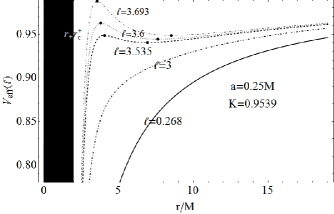
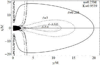
Figure 21: Effective potential $V_{eff}(\ell)$ (left-panel) and contour plot of the Boyer surfaces (sequences $\mathfrak{B}_{\ell}\equiv\mathfrak{B}_{\mathbf{p}}/\Sigma_{K}$ of “loops” of $C$, $C_{x}$ and $B$-configurations) as function of $r/M$ at fixed spin $a=0.25M\in\mathbf{BHI}$ and $K=0.9539$, and different fluid angular momentum. Each contour is at $\ell=$constant in units of mass $M$. Black region is $r<r_{+}$ ($r_{+}$ is the outer horizon), gray region is $r\in]r_{+},r_{\epsilon}^{+}]$ ($r_{\epsilon}^{+}$ is the static limit).

Configurations at $\ell_{(i)}=\ell_{(o)}$ are centered (i.e. $r^{(i)}_{min}=r^{(o)}_{min}$, $r_{min}$ being the disk center). Thus we consider here separated configurations i.e. ${C}_{(i)}\cap{C}_{(o)}=\emptyset$ or those with $y_{1}^{(i)}=y_{3}^{(o)}$, that is the critical point, (maximum of potential at $K<1$) the inner point of the outer Boyer surface or of gravitational instability where the cross occurs in the external configuration (maximum at $K>1$) coincides with the upper limit of the internal configuration, namely: ${C}_{(i)}\cap{C}_{(o)}=\{y_{1}^{(i)}\equiv y_{3}^{(o)}\}$ or ${C}_{(i)}\cap{C}_{x}^{(o)}\equiv\{y_{crit}\}$ where $y_{1}^{(i)}=y_{3}^{(o)}\equiv y_{crit}$. In this discussion we are neglecting the intersection with the inner surface that is the closest one embracing the black hole, or $y_{2}$, assuming the presence of this surface, associated to the closed configurations, does not influence the more external ones in equilibrium or the configurations $C$. The basis of this assumption relies in the fact that for each closed toroidal P-D $C$-configuration an inner surface (associated with the solution $y_{2}$), embracing the BH appears, however the two configurations are separated as far as the parameter $\mathbf{p}$ of the closed $C$-one remains far for the critical values where its morphology changes for $C$ to $C_{x}$ disk, the cross can be interpreted then as a contact point with the inner source or, in other words $y_{2}=y_{3}$, so that as far the disk is regulated by Eq. (12), that is without considering any other possible interaction due to other ingredients of the accretion disk models as the magnetic field, these two configurations at the same $\mathbf{p}$ are, far from the critical phase, separated and dynamically independent.

Thus, at $\mathbf{p}_{(i)}\neq\mathbf{p}_{(o)}$ three cases can occur: 1. $K_{(i)}=K_{(o)}$ or 2. $\ell_{(i)}=\ell_{(o)}$ or finally 3. $K_{(i)}\neq K_{(o)}$ and $\ell_{(i)}\neq\ell_{(o)}$.

The second case, 2. $\ell_{(i)}=\ell_{(o)}$, is immediately ruled out, as these are evidently centered configurations (see also Fig. (22)), at constant $\ell$ the effective potential is uniquely defined as function of $r/M$, and there is only one maximum and one minimum. For 1. $K_{(i)}=K_{(o)}$, configurations can be mutually corotating or ${\ell}$corotating, meaning here $\ell_{(i)}\ell_{(o)}>0$ or ${\ell}$counterrotating, $\ell_{(i)}\ell_{(o)}<0$, see Fig. (22), this case as well as the third 3. $K_{(i)}\neq K_{(o)}$ requires further discussion.

First, a particular but interesting case is for $\Delta_{cri}^{(i)}\cap\Delta_{cri}^{(o)}=\emptyset$, ($\Delta_{crit}\equiv[r_{Max},r_{min}]$ introduced in Sec. (IV.1)) where separated configurations can certainly exist as indeed $r_{max}^{(o)}\in I^{+}_{\mbox{\tiny{$r_{min}^{(i)}$}}}$, where $I^{+}_{\mbox{\tiny{$r_{min}^{(i)}$}}}$ is a right neighborhood of $r_{min}^{(i)}$, i.e. $r_{max}^{(o)}>r_{min}^{(i)}$ for the continuity of the effective potential there exist a point $\bar{r}^{(o)}\in I^{+}_{\mbox{\tiny{$r_{min}^{(i)}$}}}:\;\bar{r}^{(o)}<r_{Max}^{(o)}$ and it can be $\bar{r}^{(o)}=y_{1}^{(i)}$ for the configuration at $K_{(i)}=V_{eff}(p_{(i)},\bar{r})$. Thus, in conclusion a possible sufficient but not necessary condition for the formation of multiple surfaces is that $\Delta_{cri}^{(i)}\cap\Delta_{cri}^{(o)}=\emptyset$. It must be $r_{lsco}^{(i)}<r_{min}^{(i)}<r_{Max}^{(o)}<r_{lsco}^{(o)}$, this consideration clearly excludes ${\ell}$corotating matter configurations i.e. $\ell^{(o)}\ell^{(i)}>0$ (indeed $r_{b}$ and $r_{lsco}$ are functions of the black hole spin only and there are a couple of solutions $(r_{b}^{\pm},r_{lsco}^{\pm})$ for $\ell a\lessgtr 0$ respectively). For ${\ell}$counterrotating disks, $\ell^{(o)}\ell^{(i)}<0$, it has to be $r_{lsco}^{(i)}<r_{lsco}^{(o)}$. Then in conclusion multiple configurations of this kind, are necessarily ${\ell}$counterrotating and with reference to Fig. (2)-upper, it is $r_{lsco}^{(i)}=r_{lsco}^{-}$ and $r_{lsco}^{(o)}=r_{lsco}^{+}$, that is the interior surfaces must be corotating respect to the black hole ($\ell_{(i)}a>0$), and the region $[r_{min}^{(i)},r_{Max}^{(o)}]$ has to be included in $[r_{lsco}^{-},r_{lsco}^{+}]$ or $r_{lsco}^{-}<r_{min}^{-}<r_{Max}^{+}<r_{lsco}^{+}$. Furthermore from analogue consideration it follows that the maximum number of such multiple disks is $n=2$ . The range $[r_{lsco}^{-},r_{lsco}^{+}].$ increases with $a/M$ from the Schwarzschild case, where we do not distinguish multiple corotating or counterrotating configurations (meaning $\ell a\lessgtr 0$ and therefore $\ell_{(i)}\ell_{(o)}\lessgtr 0$), to the extreme Kerr case, see also Fig. (2). The region $\Delta_{crit}$ increases with the spin and the configurations can be more spaced, the innermost one approaching the black hole. However we need to distinguish between the configurations at spacetimes $a\in]0,a_{\bullet}[$ where $r_{b}^{+}<r_{lsco}^{-}$ (BHI and BHII) and the region $a\in]a_{\bullet},M[$ where $r_{b}^{+}>r_{lsco}^{-}$: in BHI and BHII there are only ${C}$-configurations. Considerations on the last bounded orbital $r_{b}^{-}$ make clear that the corotating internal configurations are necessarily closed. On the other hand, we have the double condition $\Delta_{crit}\subset[r_{b}^{+},r_{lsco}^{+}]\subset[r_{lsco}^{-},r_{lsco}^{+}]$ at $a>a_{\bullet}$, otherwise for $\Delta_{crit}\subset[r_{lsco}^{-},r_{b}^{+}]$ at $r_{Max}^{(o)}$ it is $K_{Max}^{+}>1$ and there is the possibility of outer (counterrotating) surface with a cross in $r>r_{Max}$ leading to an instability and funnel of matter in the region of the interior surface.

More generally for the existence of the separated configurations it has to be $r_{lsco}^{(i)}<r_{min}^{(i)}<r_{min}^{(o)}$, this relation also applies to the $\ell$-corotating disks and it is necessary for the existence of disjoint configurations for that it can be considered a definition for and a criterion to establish the internal and external configurations. The case $r_{Max}^{(i)}<r_{min}^{(i)}<r_{Max}^{(o)}<r_{min}^{(o)}$ has been explore above, now we focus on the case $r_{Max}^{(o)}<r_{min}^{(i)}$ (it can be $r_{Max}^{(i)}<r_{Max}^{(o)}<r_{min}^{(i)}$ or $r_{Max}^{(o)}<r_{Max}^{(i)}<r_{min}^{(i)}$). As it always exists, for definition of critical point, a closed surface centered in the minimum one can always check for two separated surfaces. But the location of the maximum $r_{Max}^{(o)}$ selects the kind of rotating matter, in fact if the disks are $\ell$corotating, $\ell_{(i)}\ell_{(o)}>0$, then it is $r_{Max}^{(o)}<r_{min}^{(i)}$, if $\ell$counterrotating, $\ell_{(i)}\ell_{(o)}<0$, then it is $r_{lsco}^{(o)}>r_{lsco}^{(i)}$ and it follows that $\ell_{(o)}>0$ (the corotating configuration respect to the black hole is the exterior one) and $\ell_{(i)}<0$ the interior configuration is counterrotating $\ell_{(i)}a<0$ and viceversa from $r_{lsco}^{(o)}<r_{lsco}^{(i)}$ it follows that $\ell_{(o)}<0$ (counterrotating $\ell_{(o)}a<0$) and $\ell_{(i)}>0$ i.e. the internal configuration is corotating respect to the black hole. For $n>2$ the necessary condition is always verified for surfaces of all $\ell$corotating matter $\ell_{i}\ell_{j}>0$, however further discussion is required for the value of the $K$-parameter.

In Figs. (22) we show a procedure to select, at different $K$, multiple separated P-D configuration, by requiring $K_{Max}^{(i)}=K_{min}^{(o)}$, the maximum number of separated configurations is $n_{Max}=4$, two of then $\ell$counterrotating, $\ell_{(i)}\ell_{(o)}<0$, and the others $\ell$corotating, $\ell_{(i)}\ell_{(o)}>0$, as shown.

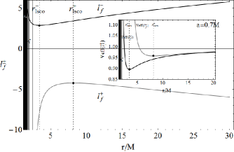
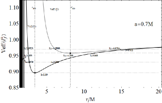
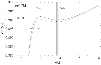
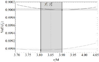
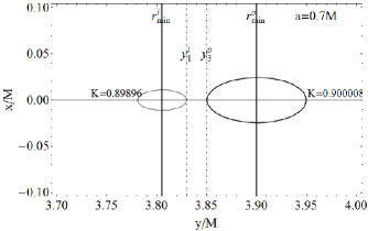
Figure 22: Fluids orbiting in a BHIV-spacetime with $a=0.7M$. Left upper panel: the fluid angular momentum $\ell_{f}^{+}$ for counterrotating (gray curve) and corotanting $\ell_{f}^{-}$ (black curve) matter as functions of the orbital radius $r/M$. Black region is $r<r_{+}$, gray region is $r\in]r_{+},r_{\epsilon}^{+}[$, the static limit is $r_{\epsilon}^{+}$, the outer horizon is the $r_{+}$. Points on the curves set the critical points of the angular momentum, located at on the last stable circular orbit $r_{lsco}^{+}$ for counterotating matter and $r_{lsco}^{-}$ for corotating matter. The marginally bounded orbits $r_{b}^{\pm}$ are also plotted. The lines at constant $K$-parameters are plotted with dotted lines. Right panel: the effective potential $V_{eff}(\ell_{f}^{+})$ for counterrotating (gray curve) and corotanting $V_{eff}(\ell_{f}^{-})$ (black curve) matter as functions of the orbital radius $r/M$, the values $V_{eff}(\ell_{f}^{\pm})$ are the $K$-parameter values of the Boyer surfaces, the values $\ell=$constant are signed with dotted lines. Center panels: Plot of $V_{eff}(\ell_{f}^{-})$ versus $r/M$. the surfaces at $K=0.90$ are for $\ell_{f}^{-}=(2.899184,2.905348)$ gray and black curves respectively. At $K=0.90$ are the maximum points $r^{\pm}_{Max}$ and the minimum $r^{\pm}_{min}$ for the two curves respectively, double (separated and closed) Boyer configurations are allowed in the gray region where $y_{3}^{(o)}$ and$y_{1}^{(i)}$ must be located: the boundaries of the region are $r_{min}$ for the outer configuration and the minimum point of the inner one (signed by a point on the gray curve) i.e. $[y_{1}^{(i)},y_{3}^{(o)}]\subset[r^{(i)}_{min},r^{(o)}_{min}]$, left panel shows a zoom of the gray region $[r^{(i)}_{min},r^{(o)}_{min}]$ as the location of $(y_{1}^{(i)},y_{3}^{(o)})$ dotted-dashed lines. Bottom panel shows the couple of corresponding Boyer surfaces, an analogue couples of configurations at $\ell=\ell_{f}^{+}$ are located at $r>4M$. The angular momentum is in units of mass $M$. These are the maximum number $(n=4)$ of $C$ configuration in this spacetime.

The case of $K_{(i)}=K_{(o)}$ is solved for any couple of fluid angular momenta $\ell_{(i)}\neq\ell_{(o)}:\;\exists!K=K_{(i)}=K_{(o)}$ where $K_{(i)}$ ($K_{(o)}$) is the effective potential associated to the inner (outer) configuration. This condition has to be completed by $r_{max}^{(i)}<r_{min}^{(i)}<y_{1}^{(i)}<y_{3}^{(o)}<y_{min}^{(o)}$ where $\left(\right)_{min}$ ($\left(\right)_{Max}$) refers as usually to the quantities at the minimum (maximum) of the effective potential. Thus it is $K_{min}^{(i)}<K<K_{Max}^{(o)}$. That is immediately verified for $\ell$corotating configurations $\ell_{(i)}\ell_{(o)}>0$. We note that in the $\ell$corotating case, $\ell_{(i)}\ell_{(o)}>0$ at fixed $r$ the effective potential increases with the magnitude of the angular momentum: $V_{eff}(\ell_{b})>V_{eff}(\ell_{a})$ as $|\ell_{b}|>|\ell_{a}|$ that is $K_{min}(\ell_{b})>K_{min}(\ell_{a})$ where $r_{lsco}^{a}=r_{lsco}^{b}$ see Fig. (23), therefore it is $r_{Max}^{a}<r_{Max}^{b}<y_{3}^{b}<y_{3}^{a}<y_{min}^{b}<y_{min}^{a}<y_{1}^{a}<y_{1}^{b}$ and they are centered configurations: $[y_{3}^{a},y_{1}^{a}]\subset[y_{3}^{b},y_{1}^{b}]$. For the $\ell$counterrotating configurations it is $r_{lsco}^{-}<r_{lsco}^{+}$, the inner configuration is corotating with respect to the source. It is necessary to distinguish the BHI-II sources at $a<a_{\bullet}:\;r_{b}^{-}<r_{b}^{+}<r_{lsco}^{-}<r_{lsco}^{+}$ and BHIII-IX $a>a_{\bullet}:\;r_{b}^{-}<r_{lsco}^{-}<r_{b}^{+}<r_{lsco}^{+}$. It is at fixed $r$ $V_{eff}^{+}>V_{eff}^{-}$, but it is required that $K_{Max}^{-}\geq K_{Max}^{+}$ and $K>K_{lsco}^{+}$ and it is always verified $r_{b}^{\pm}\leq r_{Max}^{\pm}<y_{3}^{\pm}<r_{lsco}^{\pm}<r_{min}^{\pm}<y_{1}^{\pm}$, but the assumption $y_{1}^{-}<y_{3}^{+}$ imposes the condition $r_{min}^{-}<r_{min}^{+}$ that is not satisfied as $r_{lsco}^{-}<r_{lsco}^{+}<r_{min}^{+}<r_{min}^{-}$ and $r_{max}^{-}<r_{Max}^{+}$ and $r_{min}^{+}<r_{Max}^{-}$ with $V_{eff}^{+}>V_{eff}^{-}$, see Fig. (23)

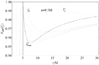
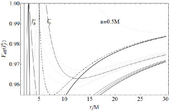
Figure 23: Effective potential $V_{eff}(\ell)$ as function of $r/M$ for a black hole spacetime at $a=0.5M\in\mathbf{BHIII}$, for different values of the fluid angular momentum $\ell_{f}^{-}$ (upper left panel), $\ell_{f}^{+}$ (upper right panel), and $\ell_{f}^{\pm}$ bottom panel, in the range $\ell\in[\ell^{\pm}_{lsco},\ell^{\pm}_{b}]$ for corotating $(-)$ and counterrotating fluids $(+)$, where $\ell^{\pm}_{lsco}\equiv\ell(r^{\pm}_{lsco})$ and $\ell^{\pm}_{b}\equiv\ell^{\pm}(r_{b})$, where $r^{\pm}_{lsco}$ the radius of the last stable circular orbits, and $r^{\pm}_{b}$ the radius of the last circular bounded orbit, the potential at $\ell_{\gamma}^{\pm}\equiv\ell_{(}r_{\gamma}^{\pm})$ has been plotted as well where $r_{\gamma}^{\pm}$ is the last circular orbit. Thick lines mark the critical points of the effective potentials. The angular momentum is in units of mass $M$.

However varying $K\in]K_{min},1[$ there may be a continuous number of many separated configurations, the pairs will denote configurations at different $K$.

We conclude this section with some final remarks: we have investigated the possible existence of a structured accretion disks defined as the union configuration $C\equiv\bigcup_{i}C_{i}$ with $C_{i}\bigcap C_{j}=\{\emptyset,y_{3},y_{1}\}$, obtained combining sub-configurations of closed or closed crossed, P-D configurations in such a way that they can be separated and not intertwined or in loops. Then we discussed some of the properties of $C_{i}$ configurations, showing that they are deeply constrained in number and in the angular momentum, so that we need to introduce the concept of $\ell$corotating and $\ell$counterrotating rings. In some cases it was proved the existence of a maximum number of separated configurations. This first analysis shows the possibility to have a multi-structured disk of a limited number of rings. Thus, the results traced here should be then completed including also the information related to the thickness and spatial distance of each sub-configurations. The dynamical equilibrium of the entire structure should be also investigated: there could arise an instability mechanism for the $C$-configuration due to the presence of one or more exterior $C_{x}$-configurations leading to a mutual destabilization (of gravitational and hydrostatic equilibrium of each torii as foreseen from the P-W model) among the sub-configurations, this mechanism imposes a limit in the number of disks, location and fluid angular momentum for the equilibrium of the multiple structurescoop .

IV.6 The polytropic equation of state and the disk morphology

We consider a polytropic equation of state assuming the pressure $p$ be a function of the matter density $\varrho$: $p=k\varrho^{\gamma}$, where $k>0$ and $\gamma$ is the polytropic index. The case of non-rotating attractor has been addressed in PuMonBe12 , mostly of the considerations traced out for $a=0$ are valid for a more generic P-W-effective potential, in particular then for $a\neq 0$. It has been shown that for the Schwarzschild geometry there is a specific classification of eligible geometric polytropics (see Raine ), and a specific class of polytropics is characterized by a discrete range of values for the index $\gamma$. A similar classification is also valid in the rotating case of the Kerr geometry. Solving Eq. (12) for $\varrho$ we find:

$$\bar{\varrho}_{\gamma}\equiv\left[\frac{1}{k}\left(V_{eff}^{-\frac{\gamma-1}{\gamma}}-1\right)\right]^{\frac{1}{(\gamma-1)}}\quad\mbox{for}\quad\gamma\neq 1,\quad\varrho_{k}\equiv V_{eff}^{-\frac{1+k}{k}}\frac{1}{1+k},\quad\mbox{for}\quad\gamma=1.$$ (47)

We adopt the normalization: $\varrho_{\gamma}\equiv k^{1/(\gamma-1)}\bar{\varrho}_{\gamma}$, which is independent from $k$.

For $\gamma=1$ it is $\varrho^{out}_{k}=\varrho^{in}_{k}\left({V^{out}_{eff}/V^{in}_{eff}}\right)^{-\frac{1+k}{k}},$ and for $\gamma\neq 1$ it is $k(\bar{\varrho})_{out}^{\gamma-1}=(k(\bar{\varrho})_{in}^{\gamma-1}+1)\left({V^{out}_{eff}/V^{in}_{eff}}\right)^{\frac{1-\gamma}{\gamma}}-1$, where the integration range $[r_{in},,r_{out}]\subset]r_{+},\infty]$ is the range of existence for $V_{eff}(\ell)$. It is $\varrho^{\prime}=0$ when $p^{\prime}=0$ and, being $\gamma>0$, the maxima (minima) of $p$ correspond to the maxima (minima) of $\varrho$. If the polytropic index is $\gamma\neq 1$ then the density $\varrho=\varrho_{\gamma}$ is: ${\varrho}_{\gamma}\equiv C^{1/(-1+\gamma)},$ with $C\equiv(V_{eff}^{-2})^{\frac{\gamma-1}{2\gamma}}-1$. We can distinguish the following two cases: 1. $C>0$ and the density $\varrho_{\gamma}$ is defined for all $\gamma$; 2. $C<0$ and the density $\varrho_{\gamma}$ is defined for $\gamma=\gamma_{q}\equiv 1+\frac{1}{2q}$, where $|q|\geq 1$ are integers- The condition $C>0$ is satisfied in two cases: where $V_{eff}^{2}<1$ and $\gamma>1$, in a range $\mathbf{R}_{\mbox{\tiny{I}}}$, and where $V_{eff}^{2}>1$ and $\gamma\in]0,1[$, in the ranges $\mathbf{R}_{\mbox{\tiny{II}}}$. When the polytropic index $\gamma=\gamma_{q}$, the fluid density $\varrho$ is defined for the conditions $\mathbf{R}_{\mbox{\tiny{I}}}\cup\mathbf{R}_{\mbox{\tiny{II}}}$, when $\gamma\neq\gamma_{q}$ it is defined only for the conditions $\mathbf{R}_{\mbox{\tiny{I}}}$.Then the only difference with the geometry $a=0$ lies in the identification of the regions $\mathbf{R}_{\mbox{\tiny{I}}}$ and $\mathbf{R}_{\mbox{\tiny{II}}}$, these are easily identifiable in the equatorial plane and are studied for the Boyer surfaces in Sec. (III.3.1). Then for the more general classes including the Boyer ${C}$-configurations, according to the analysis in Sec. (IV): $\mathbf{R}_{\mbox{\tiny{I}}}$ is $r\in]r_{+},r_{\epsilon}^{+}[$ with ${\ell}<\hat{\ell}_{\sigma}^{-}\cup\ell>\hat{\ell}_{\sigma}^{+}$ and at $r>r_{\epsilon}^{+}$ $\ell\in]\hat{\ell}_{\sigma}^{-},\hat{\ell}_{\sigma}^{+}[$, where

$$\frac{\hat{\ell}_{\sigma}^{\pm}}{M}\equiv\pm\sqrt{2}\sqrt{\frac{r\Delta\sigma^{2}\rho^{2}}{M\left(\rho^{2}-2Mr\right)^{2}}}+\frac{2ar\sigma^{2}}{2Mr-\rho^{2}},$$ (48)

(where $\sigma$ and $\rho$ are introduced in Sec. (II)) and $\mathbf{R}_{\mbox{\tiny{II}}}:$ $r\in]r_{+},r_{\epsilon}^{+}[$ with ${\ell}\in]\hat{\ell}_{\sigma}^{-},{\ell}_{\sigma}^{-}[\cup]{\ell}_{\sigma}^{+},\hat{\ell}_{\sigma}^{+}[$ and at $r>r_{\epsilon}^{+}$ ${\ell}\in]{\ell}_{\sigma}^{-},\hat{\ell}_{\sigma}^{-},[\cup]\hat{\ell}_{\sigma}^{+},{\ell}_{\sigma}^{+}[$. We can interpret these regions in terms of the orbits $r_{\kappa}^{\pm}$ in Eq. (32) and $r_{\mbox{\tiny{B}}}^{\pm}$ in Eq. (18), projecting for simplicity to the plane $\theta=\pi/2$ thus: $\mathbf{R}_{\mbox{\tiny{I}}}$: $r\in]r_{+},r_{\kappa}^{-}[\cup r>r_{\kappa}^{+}$ where $\ell\leq\ell_{b}^{+}\cup\ell>\ell_{b}^{-}$ and for $\ell\in]\ell_{b}^{-},\ell_{b}^{+}[$ it is $r>r_{+}$. and $\mathbf{R}_{\mbox{\tiny{II}}}$: $r\in]r_{\kappa}^{-},r_{\mbox{\tiny{B}}}^{-}[\cup]r_{\mbox{\tiny{B}}}^{+},r_{\kappa}^{+}[$ for $\ell<\ell_{\gamma}^{+}\cup\ell>\ell_{\gamma}^{-}$ and $r\in]r_{\kappa}^{-},r_{\kappa}^{+}[$ for $\ell\in]\ell_{\gamma}^{+},\ell_{b}^{+}[\cup]\ell_{b}^{-},\ell_{\gamma}^{-}[$.

IV.6.1 On the morphology of the Boyer surfaces

The morphology of the thick accretion disks around a Kerr attractor changes with the parameter p for, for example, the torus thickness, the disk elongation on the equatorial plane, the distance between the inner and outer surfaces of the configurations, and many properties are qualitatively poorly effected by the spin-mass ratio of the attractor PuMonBe12 . However, for $a\neq 0$ there is in general a symmetry with the respect to the transformation $\ell\rightarrow-\ell$ for different accretion disk properties, see for example Fig. (24. and we can use this fact to analyze the disk morphology in terms of the fluid angular momentum magnitude. As it is $y_{2}<y_{3}<y_{1}$ the surface maximum diameter can be defined as $\lambda(a;\mathbf{p})\equiv y_{1}-y_{3}$. For $a=0$, it increases with the $K$-parameter, but decreases with the fluid angular momentum magnitude. The situation for $a\neq 0$ is sketched in Fig. (24) where it is clear a symmetry between the $\ell$counterrotating configurations: $\lambda$ decreases with $a/M$ for corotating fluids and viceversa for the counterrotating ones.

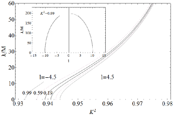
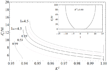
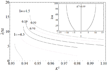
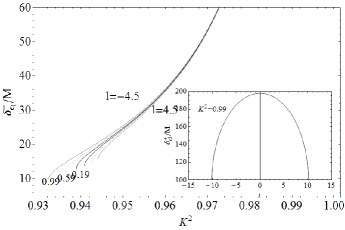
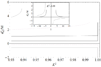
Figure 24: Plots of the function $\lambda\equiv y_{1}-y_{3}$ (left upper panel), surface of maximum torus diameter and distance from the static limit surface $\delta_{\epsilon}^{+}\equiv y_{3}-r_{\epsilon}^{+}$ (right upper panel), the distance of the torus inner surface from the structure inner surface $\hat{\delta}\equiv y_{3}-y_{2},$ (bottom panel), the distance of the structure outer surface from the horizon ${\delta}_{\epsilon_{1}}^{+}(a;\mathbf{p})\equiv y_{1}-2M$, and ${\delta}_{\epsilon_{2}}^{+}(a;\mathbf{p})\equiv y_{2}-2M$ where $y_{2}$ is the solution closest to the singularity, as functions of the parameter $K^{2}$, at different spacetime spin-mass ratios $a/M$: $a=0.99M\in\mathbf{BHIX}$ (gray curves), $a=0.59M\in\mathbf{BHIV}$ (dotted curves), $a=0.19M\in\mathbf{BHI}$ (black curves) and fluid angular momentum $\ell=-4.5$ (left set of curves) and $\ell=4.5$ (right set of curves). Inset plot shows each function of the parameter $\mathbf{p}\equiv(K,\ell)$ at fixed $K$, as function $\ell$, the black curve is for $a=10^{-5}M\in\mathbf{BHI}$, the gray curve is for $a=0.991M$. It is clear the symmetry of between the $\ell$-counterrotating configurations respect to the transformation $\ell\rightarrow-\ell$ and $\ell_{f}^{-}\rightarrow\ell_{f}^{+}$. The angular momentum is in units of mass $M$.

Then we can define the distance on inner toroidal edge from the static limit surface $r_{\epsilon}^{+}$ as: $\delta_{\epsilon}^{+}(a;\mathbf{p})\equiv y_{3}-r_{\epsilon}^{+},$ this is an increasing function of the magnitude fluid angular momentum. For corotating fluids, $\delta_{\epsilon}^{+}$ increases with $K$, and decreases with increasing $a$, at fixed $K$. For counterrotating configurations, $\delta_{\epsilon}^{+}$ increases with $K$ and $a$, see Fig. (24)-right. For some configurations it can be $\delta_{\epsilon}^{+}<0$, according with the discussion in Sec. (IV.1). The distance of the torus inner surface from the structure inner surface can be defined as $\hat{\delta}(a;\mathbf{p})\equiv y_{3}-y_{2},$ this function increases with the angular momentum magnitude and decreases with the energy. The function $\hat{\delta}(a;\mathbf{p})$ is clearly related to the unstable accretion configuration PuMonBe12 and it is therefore essential for the determination of the accretion (for $\hat{\delta}(a;\mathbf{p})=0$) and the multiple thick configurations as defined in Sec. (IV.5). Together with this, one can define as well the distance of the inner surface from the outer horizon as: $\breve{\delta}(a;\mathbf{p})\equiv y_{2}-r_{+}=\delta_{\epsilon}^{+}-\hat{\delta}+(r_{\epsilon}^{+}-r_{+}),$ for $a=0$ this quantity increases with increasing angular momentum of the fluid but decreases with increasing $K$. Finally the distance of the outer edge from the static limit ${\delta}_{\epsilon_{1}}^{+}(a;\mathbf{p})\equiv y_{1}-r_{\epsilon}^{+}$ increases with $K$, increasing as the magnitude of the angular momentum decreases. This surface is shown in Fig. (24), as function of the parameter $\ell$, it is clear the symmetry between the $\ell$counterrotating configurations. For $\ell<0$ at fixed $K$, increasing the spacetime spin $a/M$, this quantity ${\delta}_{\epsilon_{1}}^{+}$ increases on $\Sigma_{{\mathbf{p}}}$, viceversa at $\ell>0$ the function ${\delta}_{\epsilon_{1}}^{+}$ is a decreasing function of $a/M$.

We introduce the function ${\delta}_{\epsilon_{2}}^{+}(a;\mathbf{p})\equiv y_{2}-2M$ where $y_{2}$ is the solution of the problem $\mathcal{V}_{eff}=0$ closest to the singularity, it in general increases with the energy and decreases with the magnitude of the fluid angular momentum. This surface is shown in Fig. (24), notably there is a partial loss of symmetry between $\ell$couterrotating configurations. Clearly, the symmetry is lost mostly with increasing the BH spin, this fact should however not to be surprising as the properties of ${\delta}_{\epsilon_{2}}^{+}(a;\mathbf{p})$ takes into account a general constant angular momentum $\ell$ (and therefore the general symmetry $\ell\rightarrow-\ell$), but no counterrotating Boyer solutions are allowed inside the region $]r_{+},r_{\epsilon}^{+}[$ (see also discussion in Sec. (III.2.1) for some notes on the counterrotating configurations). Therefore the results traced out from Fig. (24) are valid for any general solutions of the equation $\mathcal{V}_{eff}=0$, not limited to the Boyer surfaces, and they should be read in relation to the more general surface analysis presented in Secs. (IV.2) and (IV.3).

IV.6.2 On the relativistic angular velocity

We focus now on the angular velocity $\Omega(\ell)$ on $\theta=\pi/2$ as defined in Eq. (7). $\Omega(\ell)$ increases always with the angular momentum $\ell$, i.e. $\partial_{\ell}\Omega(\ell)\nleq 0$. For a counterrotating fluid it is $\Omega_{f}^{+}\equiv\Omega(\ell_{f}^{+})<0$ the minimum of the fluid relativistic angular velocity is located in $r_{\gamma}^{+}$, that is the function $\Omega_{f}^{+}(r)$ is always increasing with the radius $r>r_{+}$, or $\partial_{r}\Omega_{f}^{+}>0$, and it is not well defined in $r_{d}$. On the other hand for $\Omega_{f}^{-}\equiv\Omega(\ell_{f}^{-})>0$ it is not well defined in $r_{d}$ and it is always decreasing with $r$, that is $\partial_{r}\Omega_{f}^{-}<0$. In general, the function $\Omega(\ell)$ has a critical point i.e. $\partial_{r}\Omega(\ell)=0$ at $\ell<0$ (minimum located at $r_{\xi}$) and for $\ell\in]a(M+r_{+})/M,\ell_{f}^{-}(r_{+})[$ (maximum located at $r_{\xi}$). For $\ell\geq\ell_{f}^{-}(r_{+})$ and $\ell\in]0,a(M+r_{+})/M]$ the function $\Omega(\ell)$, where it is defined, decreases with $r/M$ where

$$\frac{r_{\xi}}{M}\equiv 1-\frac{1}{\bar{\ell}}+2\sqrt{\frac{(\bar{\ell}-1)^{2}}{\bar{\ell}^{2}}}\cos\left(\frac{1}{3}\mbox{arcsec}\left[-\frac{2\sqrt{\frac{(\bar{\ell}-1)^{2}}{\bar{\ell}^{2}}}\bar{\ell}}{2+\bar{\ell}\left(a^{2}/M^{2}\bar{\ell}-2\right)}\right]\right).$$ (49)

V Conclusions

In this work we investigated the structure and morphology of thick accretion disks orbiting around a Kerr attractor within an hydrodynamic Polish doughnut (P-D) model. The Boyer surfaces, associated with the critical points of the effective potential, are solutions of the Euler equation. Keeping the assumption of fluid angular momentum $\ell$ constant we explored a more general class of configurations including the Boyer tori and constraining the role of the hydrostatic pressure respect to the case of a Keplerian disk. The model is regulated by the couple $\mathbf{p}=(K,\ell)$ through the fluid effective potential in the Euler equation. Sequences $\mathfrak{B}_{\mathbf{p}_{j}}\equiv\mathfrak{B}_{\mathbf{p}}/\Sigma_{\mathbf{p}_{i}}$ of corotating and counterrotating configurations are produced fixing one parameter $\mathbf{p_{i}}\in\mathbf{p}$ constant and changing the remaining $\mathbf{p}_{j}$. These collections of configurations, defined and characterized in details in the article, have been used here many times in different contexts and interpretations, providing a useful tool for the characterization of both the properties of the orbiting matter both the background spacetime. We then investigated the orbital regions where a P-D fluid configuration exist, proving that these regions depend on the gaps $\Delta_{\ell}^{\pm}(a)=\ell\pm a$, as a consequence of this it was convenient the introduction of a “rationalized” fluid momentum $\bar{\ell}\equiv\ell/a$. Studying the model in terms of the ratio $\bar{\ell}$ we identified and discussed the fluid properties determined by the dimensionless quantity $\bar{\ell}$. In particular we showed the existence, in the P-D model, of a maximum limit for $\bar{\ell}$ and in some cases the existence of these configurations is mainly determined by the ratio $\bar{\ell}$ only. According to the analysis of the P-D disks, we introduced a spacetime classification in nine sets of attractors named accordingly $\mathbf{BHI-BHIX}$. Defined by the spin-mass ratios, they are characterized by the sequences $\mathfrak{B}$: each class has a well defined and unique arrangement of the Boyer surfaces in the $\mathfrak{B}$ sequence, each slot filled with one or more configurations located in a defined orbital region, consequently the toroidal configuration analysis reveals a possible way to recognize a source from the investigation of the toroidal accreting surfaces. Finally, as the ergoregion has an important role in the of energy extraction phenomena from the black hole, during the accretions and launching of jets, especially in the magnetohydrodynamic model Meier , the cross of the static limit is then analyzed in different black hole classes. A more general class of configurations, including the P-D tori, have been also considered, these configurations turn out in different topologies not arising from the potential critical points. The array of configurations, emerged from this analysis and including the Boyer surfaces, is thus fitted within a dynamical interpretation adapted towards a possible comparison with numerical simulations of more extensive dynamic models. By varying $(\mathbf{p}_{i},\mathbf{p}_{j})\in\mathbf{p}$ we can construct a set of nine matrices $\mathfrak{B}_{\mathbf{p}}$ on the surface $\Sigma_{\mathbf{p}}\equiv\Sigma_{K}\otimes\Sigma_{\ell}$ (or $\Sigma_{K}\otimes\Sigma_{\bar{\ell}}$), each for the nine BH-class of spacetimes. The elements of $\mathfrak{B}_{\mathbf{p_{j}}}$, matrix array or column, figure different morphological phases related to the history of a single $\mathbf{p}_{i}$-disk pointing $\mathbf{p}_{j}$ as an evolutive or “chronological” parameter, meaning that we assume it to follow an evolutionary model for the configuration. The real disk evolution however can occur along a diagonal or any other sequence of elements of $\mathfrak{B}_{\mathbf{p}}$, these however could be easily fitted according to a known dynamical law or by comparison with numerical simulations: considering the matrix elements following a different order, we should recognize the matrix elements and identify then a proper exact chronological order. As accretion is usually modeled in terms of angular momentum transport inside the matter Balbus2011 ; Abramowicz:2011xu , one realistic choice for an evolutive parameter would be the fluid momentum $\ell$. The introduction of the sequences $\mathfrak{B}$ was then considered as defined on a $\Sigma_{t}$ for the analysis of multi-structured toroidal accretion disks, that is thick configurations structured in multiple P-D sub-configurations $C_{i}$ (rings), defined as the union of each closed, crossed or not torus orbiting the same attractor, whose mutual intersection is the null set or at last the inner or outer edge of the configurations. To properly define these solutions we introduced a series of concepts as the separated or intertwined sub-configurations and loops of sub-configurations, we defined then the multi-structured toroidal accretion disks as obtained combining multiple separated torus rings. Our analysis has been performed considering the situation in the nine Kerr spacetime classes. It is relevant here that, by characterizing the properties of $C_{i}$ configurations, emerged the sub-configurations are deeply constrained in number and in the angular momentum, this first analysis indeed shows the possibility in some cases of having a multi-structured disk made by a limited number of rings. Thus we introduced the concept of $\ell$corotating and $\ell$counterrotating rings. As two rings, the inner one closest to the attractor $(i)$ and the farther one $(o)$, can be mutually corotating or ${\ell}$corotating, meaning here $\ell_{(i)}\ell_{(o)}>0$ or ${\ell}$counterrotating, $\ell_{(i)}\ell_{(o)}<0$. The arrangement, in the overall structure, of the ${\ell}$corotating and ${\ell}$counterrotating rings of the same disk, is strongly constrained in the fixed class of background geometries. Then we investigated these configurations for a polytropic equation of state and analyzing the disk morphological properties in relation to the ${\ell}$counterrotating rings, as the torus thickness, the disk elongation on the equatorial plane, the distance between the inner and outer surfaces of each configuration. For $a\neq 0$, the properties of the disks, as function of $\mathbf{p}$, show a symmetry with the respect to the transformation $\ell\rightarrow-\ell$ or a symmetry between the $\ell$counterrotating configurations. Some properties of the relativistic frequency are also analyzed. This analysis is in our view a major point in this work. The results traced here we expect will be completed in a future work, investigating the different possible multi-structures not considered in the present analysis, and including also the information related to the thickness and spatial distance of each sub-configurationscoop . Thus the dynamical equilibrium of the entire structure will be then investigated: the outer sub-configurations may affect the stability of the entire structure, generating a global and internal instability phenomena, due to the presence of one or more exterior $C_{x}$-configurations. The mutual destabilization (as foreseen by the Paczyński mechanism due to of violation of the hydrostatic equilibrium) among the sub-configurations also occurs with exchange of fluid elements among the rings. This mechanism imposes indeed a limit in the number of disks, location, fluid angular momentum and thickness for the equilibrium of the multiple structures.

Appendix A Some further considerations on the effective potential

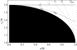
Figure 25: Plot of $r_{\mbox{\tiny{qI}}}/M$ and $r_{\mbox{\tiny{qII}}}/M$ as function of $a/M$. Black region is $r<r_{+}$, the static limit $r_{\epsilon}^{+}$, the last circular orbit $r_{\gamma}^{-}$, last bounded orbit $r_{b}^{-}$, last stable circular orbit radius $r_{lsco}^{-}$ (test particle with $L=L_{-}$) are also plotted.

Angular momentum and the energies for test particle circular orbits are

$$\frac{L_{\pm}}{\mu M}\equiv\frac{\left|\frac{a^{2}}{M^{2}}\pm 2\frac{a}{M}\sqrt{\frac{r}{M}}+\frac{r^{2}}{M^{2}}\right|}{\sqrt{\frac{r^{2}}{M^{2}}\left(\frac{r}{M}-3\right)\mp 2\frac{a}{M}\sqrt{\frac{r^{3}}{M^{3}}}}},{{E}^{(+)}_{\pm}}\equiv{{E}(L_{\pm})},\quad{{E}^{(-)}_{\pm}}\equiv{{E}(-L_{\pm})}\ .$$ (50)

for corotating $L_{-}$ ($(-)$) and counterrotating orbits $(-L_{+})$ ($(+)$) orbits. the photon orbits are and the last bounded orbits are respectively

$${r_{\gamma}^{\mp}}\equiv 2M\left(1+\cos\left[\frac{2\arccos\left(\mp\frac{a}{M}\right)}{3}\right]\right),\quad r_{b}^{\pm}\equiv 2M\pm a+2\sqrt{M}\sqrt{M\pm a},$$ (51)

the last stable circular orbits

$$r_{lsco}^{\mp}\equiv M\left(3+Z_{2}\mp\sqrt{(3-Z_{1})(3+Z_{1}+2Z_{2})}\right),$$ (52)

$Z_{1}\equiv 1+\left[1-(a/M)^{2}\right]^{1/3}\left[(1+a/M)^{1/3}+(1-a/M)^{1/3}\right]$ and $Z_{2}\equiv\sqrt{3(a/M)^{2}+Z_{1}^{2}}$.

It is $V_{eff}(\ell)=M/\ell$ (i.e. $L=\mu M$), where $a\in]0,M]$: $r\in]r_{+},r_{q}[$ and $\ell=\ell_{s}^{\pm}$, on $r=r_{q}$ and $\ell={r^{3}+a^{2}(2M+r)}/{4Ma}$, finally it is $r>r_{q},\;\ell=\ell_{s}^{+}$, where

$$\ell_{s}^{\mp}\equiv-\frac{2M^{3}a}{r\Delta-2M^{3}}\mp\sqrt{\frac{rM^{2}\Delta\left(M^{2}r+r^{3}+a^{2}(2M+r)\right)}{\left(r\Delta-2M^{3}\right)^{2}}},\quad r_{q}=1.86102M\mbox{for}\quad a/M=1/\sqrt{3},$$ (53)

$$r_{q}=r_{\mbox{\tiny{qI}}}\equiv\frac{2}{3}\left(M+\sqrt{M^{2}-3a^{2}}\cos\left[\frac{1}{3}\arccos\left[\frac{26M^{3}-9a^{3}}{\left(M^{2}-3a^{2}\right)^{3/2}}\right]\right]\right)\quad\mbox{for}\quad a/M\in[0,1/\sqrt{3}[,$$ (54)

$$r_{q}=r_{\mbox{\tiny{qII}}}\equiv-\frac{2}{3}\left(-M+\sqrt{M^{2}-3a^{2}}\sin\left[\frac{1}{3}\arcsin\left[\frac{26M^{3}-9a^{3}}{\left(M^{2}-3a^{2}\right)^{3/2}}\right]\right]\right)\quad\mbox{for}\quad a/M\in]1/\sqrt{3},1].$$ (55)

see Figs. (25).

References

- (1) B. Paczyński, P. Wiita, Astron. Astrophys. 88, 23 (1980).
- (2) B. Paczyński, Acta Astron. 30, 4 (1980).
- (3) M. Kozłowski, M. Jaroszyński, M. A. Abramowicz, Astron. Astrophys. 63, 209 (1978).
- (4) M. A. Abramowicz, M. Jaroszyński, M. Sikora, Astron. Astrophys. 63, 221 (1978).
- (5) M. A. Abramowicz, M. Calvani, L. Nobili, Astrophys. J. 242, 772 (1980).
- (6) M. Jaroszynski, M. A. Abramowicz, B. Paczynski, Acta Astronm. 30, 1 (1980).
- (7) M. A. Abramowicz, Nat. 294, 235 (1981).
- (8) M. A. Abramowicz, in Super-Eddington black hole accretion: Polish doughnuts and slim disks, A. Merloni, S. Nayakshin, R. Sunyaev, eds. ESO Astrophysics Symposia, Growing Black Holes: Accretion in a Cosmological Context. Springer-Verlag, Berlin, p. 257, (2005).
- (9) M. A. Abramowicz, A. Lanza, M. J. Percival, Astrophys. J. 479, 179 (1997).
- (10) L. G. Fishbone, V. Moncrief, Astrophys. J. 207, 962 (1976).
- (11) J. Frank, A. King, D. Raine, Accretion Power in Astrophysics, (Cambridge University Press, Cambridge 2002)
- (12) D. Pugliese, G. Montani and M. G. Bernardini, Mon. Not. R. Astron. Soc.428 (2), 952 (2013).
- (13) H. Kucakova, P. Slany, Z. Stuchlik, JCAP 01, 033 (2011).
- (14) M. A. Abramowicz, P. C. Fragile, Living Rev. Relativity 16, 1 (2013).
- (15) L. Rezzolla, O. Zanotti, J. A. Font, Astron. Astrophys. 412, 603 (2003).
- (16) Z. Stuchlik and J. Schee, Class. Quant. Grav. 29, 065002 (2012).
- (17) P. Slaný, Z. Stuchlík, Class. Quantum Gravity 22, 3623 (2005).
- (18) Z. Stuchlík, P. Slaný, AIP Conf. Proc. 861, 770 (2006).
- (19) Z. Stuchlík, P. Slaný, S. Hledík, Astron. Astrophys. 363, 425 (2000).
- (20) Z. Stuchlík, P. Slaný, J. Kovar, Class. Quantum Gravity 26, 215013, (2009).
- (21) F. H. Vincent, W. Yan, O. Straub, A. A. Zdziarski, M. A. Abramowicz, preprint (arXiv:1406.0353) (2014).
- (22) K. Ad mek and Z. Stuchl k, Class. Quant. Grav. 30, 205007 (2013).
- (23) R. Ciolfi and L. Rezzolla, Mon. Not. R. Astron. Soc. Let. 435, 1 (2013).
- (24) S. S. Komissarov, Mon. Not. R. Astron. Soc. 368, 993-1000 (2006).
- (25) J. Hamersky and V. Karas, Astron. Astrophys. 32, 555 (2013).
- (26) D. Pugliese and G. Montani, Europhys. Lett. 101, 19001 (2013).
- (27) R. H. Boyer, Proc. Camb. Phil. Soc. 61, 527 (1965).
- (28) Z. Stuchlik, A. Kotrlova and G. Torok, Astron. Astrophys. 552, A10 (2013).
- (29) W. Kluzniak and M. A. Abramowicz.preprint (arXiv:astro-ph/0105057) (2001).
- (30) W. Kluzniak and M. A. Abramowicz.preprint (arXiv:astro-ph/0203314) (2002).
- (31) M. Abramowicz, W. Kluzniak, M. Bursa, J. Hor k, P. Rebusco, G. Török, Revista Mexicana de Astronom a y Astrof sica (Serie de Conferencias) 27, 8-17 (2007).
- (32) G. Torok, A. Kotrlova, E. Sramkova, and Z. Stuchlik, Astron. Astrophys. 531, A59 7 (2011).
- (33) G. Torok, M. A. Abramowicz, W. Kluzniak, and Z. Stuchlik,Astron. Astrophys. 436, 1 8 (2005).
- (34) E. Rubio-Herrera and W. H. Lee. Mon. Not. R. Astron. Soc. 362, 789 798 (2005).
- (35) E. Rubio-Herrera and W. H. Lee, Mon. Not. R. Astron. Soc. 357, L31 L34 (2005).
- (36) Rezzolla, S. Yoshida, T. J. Maccarone, and O. Zanotti. Mon. Not. R. Astron. Soc. 344, 37-L41 (2003).
- (37) R. V. Wagoner, Astrophys. J. 752, L18 (2012).
- (38) S. Mondal Astrophys. J. 708, 1442 (2010).
- (39) A. Nagar, O. Zanotti, J. A. Font and L. Rezzolla, Phys. Rev. D 75, 044016 (2007).
- (40) Q. Lei, M. A. Abramowicz, P. C. Fragile, J. Horak, M. Machida, O. Straub, Astron. Astrophys. 498, 471 (2009).
- (41) M. A. Abramowicz, Acta. Astron. 21, 81 (1971).
- (42) S. K. Chakrabarti, Mon. Not. R. Astron. Soc. 245, 747 (1990).
- (43) S. K. Chakrabarti, Mon. Not. R. Astron. Soc. 250, 7 (1991).
- (44) S. A. Balbus, Nat. 470, 475 (2011).
- (45) N. I. Shakura, R. A. Sunyaev, Astron. Astrophys. 24, 337-355, (1973).
- (46) O.M. Blaes, Mon. Not. R. Astron. Soc. 227, 975 (1987).
- (47) M. A. Abramowicz, preprint (astro-ph/0812.3924) (2008).
- (48) J. A. Font, F. Daigne, Astrophys. J. 581, L23-L26 (2002).
- (49) M. A. Abramowicz, V. Karas, A. Lanza, Astron. Astrophys. 331, 1143 (1998).
- (50) O. M. Blaes, P. Arras, and P. C. Fragile, Mon. Not. R. Astron. Soc. 369, 1235 1252 (2006).
- (51) J. F. Hawley, Astrophys. J. 356, 580 (1990).
- (52) M. A. Abramowicz, In: Growing black holes: accretion in a cosmological context. Proceedings of the MPA/ESO/MPE/USM Joint Astronomy Conference held at Garching, Germany, 21-25 June 2004. A. Merloni, S. Nayakshin, R. A. Sunyaev (Eds.). ESO astrophysics symposia. Berlin: Springer, ISBN 3-540-25275-4, ISBN 978-3-540-25275-7, 2005, p. 257 - 273.
- (53) I. V. Igumenshchev, M. A. Abramowicz, Astrophys. J. Suppl. 130, 463 (2000).
- (54) R. Shafee, J. C. McKinney, R. Narayan, A. Tchekhovosky, C. F. Gammie, J. E. McClintock, Astrophys. J. 687, L25 (2008).
- (55) P. C. Fragile, O. M. Blaes, P. Anninois, J. D. Salmonson, Astrophys. J. 668, 417-429 (2007).
- (56) J-P. De Villiers, J. F. Hawley, Astrophys. J. 577, 866 (2002).
- (57) J. F. Hawley, Mon. Not. R. Astron. Soc. 225, 677 (1987).
- (58) J. F. Hawley, Astrophys. J. 381, 496 (1991).
- (59) J. F. Hawley, L. L. Smarr, J. R. Wilson, Astrophys. J. 277, 296 (1984).
- (60) Z. Stuchlík, J. Kovář , Int. J. Mod Phys D, 17 (2008).
- (61) J. A. Font, Living Rev. Relat., 6, 4 (2003).
- (62) C. W. Misner, K. S. Thorne, J. A. Wheeler, Gravitation, (Freeman, San Francisco, 1973).
- (63) S. Chandrasekhar, The mathematical theory of Black Holes, (International Series of Monographs on Physics, Hardcover, 1983).
- (64) R. Ruffini, in Black Holes Les Astres Occlus, edited by C. DeWitt and B. S. DeWitt (Gordon and Breach, New York, 1973).
- (65) D. Pugliese, H. Quevedo and R. Ruffini, Phys. Rev. D 84 044030 (2011).
- (66) B. Aschenbach, Astron. Astrophys. 425, 1075 (2004).
- (67) Z. Stuchlik, P. Slany, G. Torok and M. A. Abramowicz, Phys. Rev. D 71, 024037 (2005).
- (68) B. O’Neill, The Geometry of Kerr Black Holes, (A. K. Peters, Wellesley, Massachusetts, 1995).
- (69) D. L. Meier, Black Hole Astrophysics The Engine Paradigm, (Springer-Verlag, Berlin Heidelberg, 2012).
- (70) D. Pugliese and H. Quevedo, preprint (arXiv:1409.7652) (2014).
- (71) in preparation.