Comparing Monte Carlo methods for finding ground states of Ising spin glasses:
Population annealing, simulated annealing, and parallel tempering

Abstract

Population annealing is a Monte Carlo algorithm that marries features from simulated-annealing and parallel-tempering Monte Carlo. As such, it is ideal to overcome large energy barriers in the free-energy landscape while minimizing a Hamiltonian. Thus, population-annealing Monte Carlo can be used as a heuristic to solve combinatorial optimization problems. We illustrate the capabilities of population-annealing Monte Carlo by computing ground states of the three-dimensional Ising spin glass with Gaussian disorder, while comparing to simulated-annealing and parallel-tempering Monte Carlo. Our results suggest that population annealing Monte Carlo is significantly more efficient than simulated annealing but comparable to parallel-tempering Monte Carlo for finding spin-glass ground states.

I Introduction

Spin glasses present one of the most difficult challenges in statistical physics Stein and Newman (2013). Finding spin-glass ground states is important in statistical physics because some properties of the low-temperature spin-glass phase can be understood by studying ground states. For example, ground-state energies in different boundary conditions have been used to compute the stiffness exponent of spin glasses Carter et al. (2002); Hartmann (1999); Hukushima (1999). More generally, the problem of finding ground states of Ising spin glasses in three and more dimensions is a nnondeterministic polynomial-time (NP) hard combinatorial optimization problem Barahona (1982) and is thus closely related to other hard combinatorial optimization problems Moore and Mertens (2011), such as protein folding Trebst et al. (2006) or the traveling salesman problem. As such, developing efficient algorithms to find the ground state of a spin-glass Hamiltonian—as well as related problems that fall into the class of “quadratic unconstrained binary optimization problems”—represents an important problem across multiple disciplines.

Many generally applicable computational methods have been developed to solve hard combinatorial optimization problems. Exact algorithms that efficiently explore the tree of system states include branch-and-cut Simone et al. (1995) algorithms. Heuristic methods include genetic algorithms Hartmann and Rieger (2001, 2004), particle swarm optimization Bǎutu and Bǎutu (2008), and extremal optimization Boettcher and Percus (2001); Middleton (2004). The focus of this paper is on heuristic Monte Carlo methods based on thermal annealing approaches. In particular, we studied simulated annealing Kirkpatrick et al. (1983), parallel-tempering Monte Carlo Swendsen and Wang (1986); Geyer (1991); Hukushima and Nemoto (1996), and population-annealing Monte Carlo Hukushima and Iba (2003). The first two methods are well-known and have been successfully applied to minimize Hamiltonians, while the third has been much less widely used in statistical physics and a primary purpose of this paper is to introduce population annealing as an effective method for finding ground states of frustrated disordered spin systems.

Population-annealing Monte Carlo Hukushima and Iba (2003); Machta (2010); Machta and Ellis (2011); Zhou and Chen (2010); Wang et al. (2014) is closely related to simulated annealing and also shares some similarities with parallel tempering. Both simulated annealing and population annealing involve taking the system through an annealing schedule from high to low temperature. Population annealing makes use of a population of replicas of the system that are simultaneously cooled and, at each temperature step, the population is resampled so it stays close to the equilibrium Gibbs distribution. The resampling step plays the same role as the replica exchange step in parallel-tempering Monte Carlo. On the other hand, population annealing is an example of a sequential Monte Carlo algorithm Doucet et al. (2001), while parallel tempering is a Markov chain Monte Carlo algorithm. In a recent large-scale study Wang et al. (2014), we have thoroughly tested population-annealing Monte Carlo against the well-established parallel tempering-Monte Carlo method. Simulations of thousands of instances of the Edwards-Anderson Ising spin glass show that population annealing Monte Carlo is competitive with parallel-tempering Monte Carlo for doing large-scale spin-glass simulations at low but nonzero temperatures where thermalization is difficult. Not only is population-annealing Monte Carlo competitive in comparison to parallel-tempering Monte Carlo when it comes to speed and statistical errors, it has the added benefits that the free energy is readily accessible, multiple boundary conditions can be simulated at the same time, the position of the temperatures in the anneal schedule does not need to be tuned with as much care as in parallel tempering, and it is trivially parallelizable on multi-core architectures.

It is well known that parallel tempering is more efficient at finding spin-glass ground states than simulated annealing Romá et al. (2009); Moreno et al. (2003) because parallel tempering is more efficient at overcoming free-energy barriers. Here we find that population annealing is comparably efficient to parallel tempering Monte Carlo and, thus, also more efficient than simulated annealing. Nonetheless, because of the strong similarities between population annealing and simulated annealing, a detailed comparison of the two algorithms is informative and sheds light on the importance of staying near equilibrium, even for heuristics designed to find ground states.

The outline of the paper is as follows. We first introduce our benchmark problem, the Edwards-Anderson Ising spin glass, and the population annealing algorithm in Sec. II. We then study the properties of population annealing for finding ground states of the Edwards-Anderson model and compare population annealing with simulated annealing in Sec. III.2. We conclude by comparing the efficiency of population annealing and parallel tempering in Sec. IV and present our conclusions in Sec. V.

II Models and Methods

II.1 The Edwards-Anderson model

The Edwards-Anderson (EA) Ising spin-glass Hamiltonian is defined by

$$\mathcal{H}=-\sum\limits_{\langle ij\rangle}J_{ij}s_{i}s_{j},$$ (1)

where $s_{i}=\pm 1$ are Ising spins on a $d$-dimensional hypercubic lattice with periodic boundary conditions of size $N=L^{3}$. The summation $\langle ij\rangle$ is over all nearest neighbor pairs. The couplings $J_{ij}$ are independent Gaussian random variates with mean zero and variance one. For Gaussian disorder, with probability one, there is a unique pair of ground states for any finite system. We call a realization of the couplings $\{J_{ij}\}$ a sample. Here we study the three-dimensional (3D) EA model.

II.2 Population Annealing and Simulated Annealing

Population annealing (PA) and simulated annealing (SA) are closely related algorithms that may be used as heuristics to find ground states of the EA model. Both algorithms change the temperature of a system through an annealing schedule from a high temperature where the system is easily thermalized to a sufficiently low temperature where there is a significant probability of finding the system in its ground state. At each temperature in the annealing schedule $N_{S}$ sweeps of a Markov-chain Monte Carlo algorithm are applied at the current temperature. The annealing schedule consists of $N_{T}$ temperatures. The ground state is identified as the lowest-energy configuration encountered during the simulation.

Population annealing differs from simulated annealing in that a population of $R$ replicas of the system are cooled in parallel. At each temperature step there is a resampling step, described below.

The resampling step in PA keeps the population close to the Gibbs distribution as the temperature is lowered by differentially reproducing replicas of the system depending on their energy. Lower-energy replicas may be copied several times and higher-energy replicas eliminated from the population. Consider a temperature step in which the temperature $T=1/\beta$ is lowered from from $\beta$ to $\beta^{\prime}$, where $\beta^{\prime}>\beta$. The reweighting factor required to transform the Gibbs distribution from $\beta$ to $\beta^{\prime}$ for replica $i$ with energy $E_{i}$ is $e^{-(\beta^{\prime}-\beta)E_{i}}$. The expected number of copies $\tau_{i}(\beta,\beta^{\prime})$ of replica $i$ is proportional to the reweighting factor

$$\tau_{i}(\beta,\beta^{\prime})=\dfrac{e^{-(\beta^{\prime}-\beta)E_{i}}}{Q(\beta,\beta^{\prime})},$$ (2)

where $Q$ is a normalization factor that keeps the expected population size fixed,

$$Q(\beta,\beta^{\prime})=\frac{1}{R}\sum\limits_{i=1}^{R_{\beta}}e^{-(\beta^{\prime}-\beta)E_{i}}.$$ (3)

Here $R_{\beta}$ is the actual population size at inverse temperature $\beta$. A useful feature of PA is that the absolute free energy can be easily and accurately computed from the sum of the logarithm of the normalizations $Q$ at each temperature step. Details can be found in Ref. Machta (2010).

Resampling is carried out by choosing a number of copies to make for each replica in the population at $\beta^{\prime}$. There are various ways to choose the integer number of copies $n_{i}(\beta,\beta^{\prime})$ having the correct (real) expectation $\tau_{i}(\beta,\beta^{\prime})$. The population size can be fixed ($R_{\beta}=R$) by using the multinomial resampling Machta and Ellis (2011) or residual resampling Douc and O.Cappé (2005). Here we allow the population size to fluctuate slightly and use nearest-integer resampling. We let the number of copies be $n_{i}(\beta,\beta^{\prime})=\lfloor\tau_{i}(\beta,\beta^{\prime})\rfloor$ with probability $\lceil\tau_{i}(\beta,\beta^{\prime})\rceil-\tau_{i}(\beta,\beta^{\prime})$ and $n_{i}(\beta,\beta^{\prime})=\lceil\tau_{i}(\beta,\beta^{\prime})\rceil$, otherwise. $\lfloor x\rfloor$ is the greatest integer less than $x$ and $\lceil x\rceil$ is least integer greater than $x$. This choice insures that the mean of $n_{i}(\beta,\beta^{\prime})$ is $\tau_{i}(\beta,\beta^{\prime})$ and the variance is minimized.

The resampling step ensures that the new population is representative of the Gibbs distribution at $\beta^{\prime}$ although for finite population $R$, biases are introduced because the low-energy states are not fully sampled. In addition, the population is now correlated due to the creation of multiple copies. Both of these problems are partially corrected by carrying out Metropolis sweeps and the undersampling of low-energy states is reduced by increasing $R$. Indeed, for PA, which is an example of a sequential Monte Carlo method Doucet et al. (2001), systematic errors are eliminated in the large-$R$ limit. By contrast, for PT, which is a Markov-chain Monte Carlo method, such systematic errors are eliminated in the limit of a large number of Monte Carlo sweeps.

In all our PA and SA simulations, the annealing schedule consists of temperatures that are evenly spaced in $\beta=1/T$ with the highest temperature $1/T=\beta=0$ and the lowest temperature $1/T=\beta=5$. The Markov chain Monte Carlo is the Metropolis algorithm and, unless otherwise stated, there are $N_{S}=10$ Metropolis sweeps at each temperature.

For both PA and SA the ground state is presumed to be the lowest energy spin configuration encountered at the end of the simulation. For SA it is most efficient to do multiple runs and choose the lowest energy from among the runs rather than do one very long run. Thus, the SA results are typically stated as a function of the number of runs $R$. Population annealing is inherently parallel and we report results for a single run with a population size $R$. Indeed, choosing the minimum energy configuration among $R$ runs of SA is equivalent to running PA with the same population size but with the resampling step turned off, which justifies using the same symbol $R$ to describe the population size in PA and the number of runs in SA.

While population annealing is primarily designed to sample from the Gibbs distribution at nonzero temperature, here we are interested in its performance for finding ground states. We test the hypothesis that the resampling step in PA improves ground-state searches as compared to SA. The motivation for this hypothesis is that the resampling step removes high-energy spin configurations and replaces them with low-energy configurations, thus potentially increasing the probability of finding the ground state for a given value of $R$.

The equilibration of population annealing can be quantified using the family entropy of the simulation. A small fraction of the initial population has descendants in the final population at the lowest temperature. Let $\nu_{i}$ be the fraction of the final population at the lowest temperature descended from replica $i$ in the initial population. Then the family entropy $S_{f}$ is given by

$$S_{f}=-\sum_{i}\nu_{i}\log\nu_{i}.$$ (4)

The exponential of the family entropy is an effective number of surviving families. A high family entropy indicates smaller statistical and systematic errors and can be used as a thermalization criterion for the method.

II.3 Measured quantities

To compare PA and SA we investigated the following quantities. For PA let $g(R)$ be the fraction of the population in the ground state for a run with population size $R$. It is understood that $g$ is measured at the lowest simulated temperature. Clearly, the quantity $g(1)$ is simply the probability of finding the ground state in a single run of SA. Let $\mathcal{P}(R)$ be the probability of finding the ground state in a run with population size $R$. For SA, $\mathcal{P}_{\rm SA}(R)$ is the probability of finding the ground state in $R$ independent runs, i.e.,

$$\mathcal{P}_{\rm SA}(R)=1-[1-g(1)]^{R}.$$ (5)

However, for PA the resampling step tends to reproduce discoveries of the ground state so that the probability $\mathcal{P}_{\rm PA}(R)$ is less than the result for $R$ independent searches. What we actually measured is $N_{0}$, the number of occurrences of the ground state in the population from which we obtained $g(R)=N_{0}/R$ in the case of PA and $g(1)$ in the case of SA.

In the limit of large $R$, PA generates an equilibrium population described by the Gibbs distribution so

$$\lim_{R\rightarrow\infty}g(R)=g_{0},$$ (6)

where $g_{0}$ is the fraction of the ensemble in the ground state,

$$g_{0}=\frac{1}{Z(\beta)}2e^{-\beta E_{0}}=2e^{-\beta E_{0}+\beta F(\beta)},$$ (7)

where $E_{0}$ is the ground-state energy, $Z(\beta)$ is the partition function and $F(\beta)=-\log[Z(\beta)]/\beta$ is the Helmholtz free energy. As explained in Refs. Machta (2010); Wang et al. (2014, (2014), PA yields accurate estimates for the Helmholtz free energy based on the normalization factors $Q(\beta,\beta^{\prime})$ defined Eq. (3). Thus, we have an independent prediction for the limiting value of $g(R)$.

We considered two disorder-averaged quantities as well. The first is the probability of finding the ground state, averaged over disorder samples,

$$\eta=\overline{\mathcal{P}},$$ (8)

where the overbar indicates a disorder average. The quantity $\eta$ is the primary measure we used to compare the three algorithms.

The second quantity, $\alpha$, is a disorder-averaged measure of accuracy of finding the ground-state energy, i.e.,

$$\alpha=1-\overline{(E_{\rm min}/E_{0})},$$ (9)

where $E_{\rm min}$ is the minimum energy found in the simulation, which might not be the true ground-state energy $E_{0}$.

III Results

III.1 Finding ground states with population annealing

To compare population annealing and simulated annealing, we need a collection of samples with known ground-state energies. In Ref. Wang et al. (2014) we reported on a simulation of approximately $5000$ samples of the 3D EA spin glass for size $L=4$, $6$, $8$, and $10$ using large population runs of PA. Note that these sizes are typical of recent ground-state studies of spin glasses. Ground-state energies were obtained from these runs by taking the lowest energy encountered in the population at the lowest temperature, $\beta=5$, using more-than-adequate resources. We used the data from this large-scale simulation as the reference ground-state energy for each sample and compared the same set of samples for smaller PA runs and for SA runs. The population size and number of temperature steps in the reference data set are shown in Table 1. Our PAimplementation uses OPENMP and each simulation runs on eight cores.

Table 1: Simulation parameters of the reference simulations of Ref. Wang et al. (2014) from which ground states were obtained. $L$ is the linear system size, $R$ is the population size, $N_{T}$ is the number of temperatures in the annealing schedule, $\min(N_{0})$ is the minimum with respect to samples of the number of replicas in the ground state.

$L$	$R$	$N_{T}$	$\min(N_{0})$
4	5$\times 10^{4}$	101	3370
6	2$\times 10^{5}$	101	1333
8	5$\times 10^{5}$	201	172
10	1$\times 10^{6}$	301	2

Population annealing, like simulated annealing and parallel tempering, is a heuristic method and it is not guaranteed to find the ground state except in the limit of an infinite population size. Nonetheless, we have confidence that we have found the ground state for all or nearly all samples. For an algorithm like PA that is designed to sample the Gibbs distribution at low temperature, the question of whether the true ground state has been found is closely related to the question of whether equilibration has been achieved at the lowest simulated temperature. The candidate ground state is defined as the minimum energy state in the population at the lowest temperature $\beta$. For an equilibrium ensemble, the fraction of the ensemble in the ground $g_{0}$ is given by the Gibbs distribution, Eq. (7). If the number of copies of the found ground state in the low-temperature population $N_{0}$ is large and if the population is in equilibrium, then it is unlikely that the true ground-state energy has not been found. Because, if we have not found the true ground state, the number of copies of the true ground state, $Rg_{0}$, would be expected to be even larger than $N_{0}$. Thus, if we believe the population is in equilibrium at low temperature and if the candidate ground state is found many times in the low-temperature population, then we have high confidence that the candidate is the true ground state.

Of course, it cannot be guaranteed that the population generated by PA is in equilibrium at low temperature. However, the production runs from which we measured ground-state energies passed a stringent thermalization test. We required a large effective number of independent families based on the family entropy, defined in Eq. (4). We required $e^{S_{f}}\geq 100$; additional runs were done for those samples that did not meet these criteria. We also compared our results for the same set of samples to results reported in Ref. Yucesoy (2013) using parallel tempering Monte Carlo. We found good agreement for both averaged quantities and the overlap distribution for individual samples.

In addition to the equilibration test, we recorded the number of copies of the ground state in the population at the lowest temperature and found that for most samples this number is large. A histogram of $N_{0}/R=g(R)\approx g_{0}$ of all samples is given in Fig. 1 for each system size $L$. The minimum value of $N_{0}$ for each system size is shown in Table 1. For the small fraction ($0.7$%) of $L=10$ samples with $N_{0}<10$ we re-ran PA with a $10$-fold larger population, $R=10^{7}$. In no case did the ground-state energy change. In addition, for the one sample with $N_{0}=2$ we confirmed the ground state using an exact branch and cut algorithm run on the University of Cologne Spin Glass Server sgs . Based on the strict equilibration criteria and the large number of ground states reported in Table 1, we are confident that we have found true ground states for all samples.

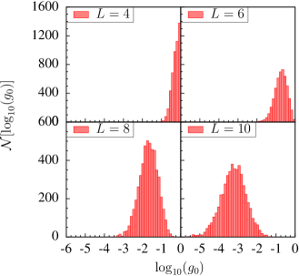
Figure 1: (Color online) Histogram of the number of samples with fraction in the ground state $g_{0}$ at $\beta=5$ for various sizes $L$, estimated from the reference runs described in Table 1. $\mathcal{N}[\log_{10}(g_{0})]$ is the number of samples in the logarithmic bin centered at $\log_{10}(g_{0})$. There are a total of $50$ bins. Note that as $L$ increases, the histograms shift rapidly to smaller values.

As an additional check, we compared the disorder-averaged ground-state energy per spin against values in the literature using the hybrid genetic algorithm Palassini and Young (1999) and parallel tempering (PT) Romá et al. (2009). The comparison is shown in Table 2 and reveals that all three methods yield the same average energy within statistical errors.

Table 2: Comparison of the disorder averaged ground-state energy per spin for the EA model with those obtained from the hybrid genetic algorithm Palassini and Young (1999) and PT Romá et al. (2009).

$L$	PA	Hybrid genetic	PT
4	-1.6639(14)	-1.6655(6)	-1.6660(2)
6	-1.6899(7)	-1.6894(5)	-1.6891(4)
8	-1.6961(5)	-1.6955(4)	-1.6955(6)
10	-1.6980(3)	-1.6975(5)	-1.6981(7)

A striking feature of Fig. 1 is that the fraction of the ensemble in the ground state $g_{0}$ decreases rapidly as $L$ increases. Thus, for any temperature-based heuristic, including PA, SA, and PT, it is necessary to simulate at lower temperatures and/or use larger populations (or, for PT, longer runs) as $L$ increases. To understand this requirement more formally we rewrite Eq. (7) in terms of intensive quantities

$$g_{0}=2\exp[-N\beta(e_{0}-f(\beta))],$$ (10)

where $e_{0}$ and $f(\beta)$ are the ground-state energy and free energy per spin, respectively, and $N=L^{3}$ is the number of spins. In the thermodynamic limit, $[e_{0}-f(\beta)]$ is expected to converge to a positive number that is independent of the disorder realization. Thus, for fixed $\beta$, the fraction of the ensemble in the ground state decreases exponentially in the system size.

As discussed in Sec. II.2, population annealing gives a direct estimator of the free energy, thus we can independently measure all of the quantities in Eq. (7) and carry out a disorder average. Because the observables on the right-hand side of Eq. (7) appear in the exponent, it is convenient to take the logarithm and then carry out the disorder average. Table 3 compares $\overline{\log_{10}g_{0}}$ and $\log_{10}2-\beta\overline{(E_{0}-F)}/\log(10)$ at $\beta=5$. The table confirms the expected equilibrium behavior of the fraction in the ground state. Note that the observables $g_{0}$, $E_{0}$, and $F$ are not entirely independent quantities, which explains why the statistical errors are significantly larger than the difference in the values. On the other hand, if the simulation was not in thermal equilibrium, these quantities would not agree.

Table 3: Comparison of the disorder average of the log of the two sides of Eq. (7) at $\beta=5$.

$L$	$\overline{\log_{10}g_{0}}$	$\log_{10}2-\beta\overline{(E_{0}-F)}/\log(10)$
4	-0.2644(28)	-0.2643(28)
6	-0.7573(46)	-0.7563(46)
8	-1.6933(77)	-1.6925(67)
10	-3.2358(104)	-3.2297(91)

For all the reasons discussed above we believe that we have found the true ground state for all samples. However, our main conclusions would not be affected if a small fraction of the reference ground states are not true ground states.

III.2 Comparison between population annealing and simulated annealing

III.2.1 Detailed comparison for a single sample

In this section we present a comparison of population annealing and simulated annealing for a single disorder realization. This sample was chosen to be hardest to equilibrate for $L=8$ based on having the smallest family entropy [see Eq. (4)]; however, it has a probability of being in the ground state at the lowest temperature near the average for size $L=8$. For this sample we confirmed the ground-state energy found in the reference PA run using the University of Cologne Spin Glass Server sgs .

Figure 2 shows the fraction of the population in the ground state $g(R)$ as a function of population size $R$ for PA. The result for the probability that SA has found the ground state in a single run is simply the value at $R=1$. In this simulation, we used $N_{T}=101$ temperatures with $N_{S}=10$ sweeps per temperature for both algorithms. It is striking that the fraction of ground states in the population increases by about four orders of magnitude from the small value for SA, $g(1)$ to the limiting value for PA for large $R$, $g(10^{6})\approx g_{0}$. This result shows that resampling greatly increases the probability that a member of the PA population is in the ground state. It suggests that even though equilibration is not required for finding ground states, the probability of finding the ground state is improved when the simulation is maintained near thermal equilibrium. Of course, remaining near equilibrium as the temperature is lowered is also a motivation for SA but lacking the resampling step, SA falls out of equilibrium once the free-energy landscape roughness significantly exceeds $k_{\rm B}T$. However, the ratio of $g(R)/g(1)$ is an overestimate of the ratio the probabilities for actually finding the ground state for a fixed $R$ because once the ground state is discovered in PA, it is likely to be reproduced many times.

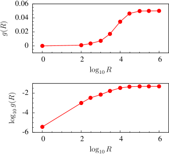
Figure 2: (Color online) The fraction of the population in the ground state $g(R)$ as a function of population size $R$ for a single sample using PA with $N_{T}=101$ and $N_{S}=10$. The point at $\log_{10}R=0$ corresponds to the probability that a single run of SA will yield the ground state. The upper panel is a log-linear plot and the lower panel is a log-log plot of the same data. Error bars are smaller than the symbols.

The probability of finding the ground state $\mathcal{P}$ for a given amount of computational work is an appropriate metric to compare the two algorithms. We measured the amount of work $W$ in Metropolis sweeps, $W=RN_{T}N_{S}$. In most of our comparisons we used the same value of $N_{T}$ and $N_{S}$ for both PA and SA. However, it is not clear whether the two algorithms are optimized with the same values of $N_{T}$ and $N_{S}$. We performed additional optimization of SA varying $N_{T}$ and $N_{S}$. We used the computational work divided by the probability of finding the ground state in a single SA run, with $N_{T}N_{S}/g$ as a figure of merit. Note that in the relevant large-$R$ regime, minimizing $N_{T}N_{S}/g$ is equivalent to maximizing $\mathcal{P}$ for a fixed amount of work. Figure 3 shows $N_{T}N_{S}/g$ versus $N_{T}N_{S}$ and reveals a broad minimum near $N_{T}N_{S}\approx 5\times 10^{3}$. We therefore performed SA simulations at the same value used for PA, $N_{T}N_{S}=1010$, and a more nearly optimal value, $N_{T}N_{S}=5000$. Note that for SA it is only the product, $N_{T}N_{S}$, that determines the efficiency, not $N_{T}$ and $N_{S}$ separately. Note also that the efficiency decreases when $N_{T}N_{S}$ is too large, suggesting that it is better to do many shorter SA runs rather than a single long run.

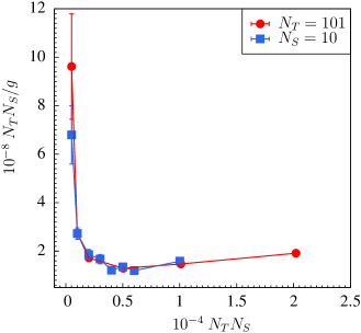
Figure 3: (Color online) The computational work divided by the probability of finding the ground state in a single SA run, $N_{T}N_{S}/g$ vs the computational work $N_{T}N_{S}$ for a single sample. The two curves correspond to holding $N_{S}=10$ fixed and varying $N_{T}$ (blue squares) and holding $N_{T}=101$ fixed and varying $N_{S}$ (red circles). Smaller values of $N_{T}N_{S}/g$ correspond to more efficient simulations.

Figure 4 compares $\mathcal{P}_{\rm SA}$, obtained from Eq. (5), and $\mathcal{P}_{\rm PA}(R)$, obtained from multiple runs of PA as a function of the computational work $W$. In this simulation we used $N_{T}=101$ temperatures with $N_{S}=10$ for PA and the lower SA curve. The upper SA curve corresponds to the optimal value $N_{T}N_{S}=5000$. Computational work was varied by changing $R$ holding $N_{T}$ and $N_{S}$ fixed. For intermediate values of $R$, corresponding to realistic simulations, $\mathcal{P}_{\rm PA}$ exceeds $\mathcal{P}_{\rm SA}$ by one or two orders of magnitude and the amount of work needed to be nearly certain of finding the ground is also more than an order of magnitude less for PA than SA. Note that the effect of optimizing SA is only about a factor of $2$. We conclude that for this sample, there is a large difference in efficiency between PA and SA and this difference cannot be explained by a difference in the optimization of the two methods. To see whether this difference is typical and how it depends on system size, in Sec. III.2.2 we consider averages over disorder realizations.

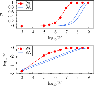
Figure 4: (Color online) Probability of finding the ground state $\mathcal{P}$ as a function of the computational work $W=RN_{T}N_{S}$ for a single sample for both SA and PA. The computational work is varied by changing population size $R$, holding $N_{T}N_{S}$ fixed. For PA and the lower SA curve, $N_{T}N_{S}=1010$ while for the upper SA curve, $N_{T}N_{S}=5000$, which is near the optimum value for SA. The upper panel is a log-linear plot and the lower panel is a log-log plot. Error bars for PA are smaller than the symbols. The SA curves are obtained from Eq. (5).

III.2.2 Disorder-averaged comparison

We compared population annealing and simulated annealing for approximately $5000$ disorder realizations for each of the four system sizes, $L=4$, $6$, $8$, and $10$, and for several different population sizes. For SA the population size refers to the number of independent runs. Both algorithms use the same annealing schedule with evenly spaced inverse temperatures starting with infinite temperature and ending at $T_{0}=0.2$. The number of sweeps per temperature is $N_{S}=10$. The population sizes $R$, number of temperatures in the annealing schedule $N_{T}$, the number of disorder realizations $M$ and the corresponding parameters for the reference runs are given in Table 4.

Table 4: Parameters of the numerical simulations for comparison between PA and SA. $R$ is the population size, $N_{T}$ is the number of temperatures, and $M$ is the number of samples studied. The reference parameters are for the PA runs used to estimate the ground-state energy for each sample.

$L$	$\log_{10}R$	$N_{T}$	$M$	Ref. $R$	Ref. $N_{T}$
4	{1,2,3,4}	101	4941	5$\times 10^{4}$	101
6	{1,2,3,4,5}	101	4959	2$\times 10^{5}$	101
8	{1,2,3,4,5}	101	5099	5$\times 10^{5}$	201
10	{1,2,3,4,5}	201	4945	1$\times 10^{6}$	301

Figure 5 shows $\alpha$, the disorder averaged error in finding the ground state [see Eq. (9)], as function of population size $R$ for SA and PA. For small systems neither algorithm makes significant errors even for small populations but as the system size increases, PA is significantly more accurate.

Figure 6 shows $\eta$, the disorder-averaged fraction of samples for which the ground state is found [see Eq. (8)], as a function of population size $R$. Again, we see that for $L=4$ and $6$, the two algorithms are comparable but for $L=8$ and $10$, population annealing is far more likely to find the ground state for the same population size. It is clear from Figs. 5 and 6 that population annealing is both more accurate and more efficient at finding ground states than simulated annealing and that as system size increases, the relative advantage of PA over SA increases.

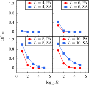
Figure 5: (Color online) Error in approximating the the ground-state energy ($\alpha$) vs log population size, $\log_{10}(R)$.

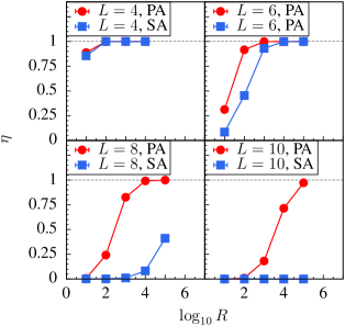
Figure 6: (Color online) Fraction of samples for which the ground state is found ($\eta$) vs log population size, $\log_{10}(R)$ for population annealing and simulated annealing.

IV Comparison between Population Annealing and Parallel Tempering

In this section, we compare the efficiency of population annealing (PA) and parallel tempering (PT) when finding ground states. We first briefly describe parallel-tempering Monte Carlo. Parallel tempering simultaneously simulates $N_{T}$ replicas of the system at $N_{T}$ different temperatures. In addition to single-temperature Metropolis sweeps, PA uses replica exchange moves in which two replicas at neighboring temperatures swap temperatures. To satisfy detailed balance, the swap probability $p_{\rm swap}$ is given by

$$p_{\rm swap}=\min\Big{[}1,\exp\left[(\beta^{\prime}-\beta)(E^{\prime}-E)\right]\Big{]},$$ (11)

where $E$ and $E^{\prime}$ are the energies of the replicas proposed for exchange at temperatures $\beta$ and $\beta^{\prime}$, respectively.

Results for PT are taken from Romá et al. Romá et al. (2009), who studied the disorder-averaged probability of finding the ground state $\eta$ for the 3D EA model for the same sizes considered here. They gave an empirical fit of their data of the form,

$$\eta=\dfrac{e^{qx}}{1+e^{qx}},$$ (12)

where $q$ is a fitting parameter and $x$ is a function of the computational work $W$ and system size $L$ defined as

$$x=[\log(W/2)-(bL^{c}-a)]/L^{d},$$ (13)

and the work is calculated in units of Monte Carlo sweeps. For PT, the computational work is given by $W=N_{T}N_{S}$ while for PAit is given by $W=RN_{T}N_{S}$. We assume that the work involved in replica exchange moves for PT and in population resampling for PA is negligible compared to the work associated with the Metropolis sweeps. The fitting parameters for the 3D EA model reported in Ref. Romá et al. (2009) are $a=-0.05$, $b=1.55$, $c=1$, $d=0.2$, and $q=2$.

Figure 7 shows $\eta$, the fraction of samples for which the ground state is correctly found versus the scaled work $x$ for our PA data (points) and the fit for PT from Romá et al. (2009) (solid curve). It is striking that both algorithms perform nearly identically over the whole range of sizes and amounts of computational work.

Figure 7: (Color online) Fraction of samples for which the ground state is found ($\eta$) as a function of the scaled computational work $x$ [Eq. (13)] for both population annealing and parallel tempering. The curve is taken from the empirical fit [Eq. (12)] of Ref. Romá et al. (2009).

V Conclusion

We have carried out a detailed comparison of three Monte Carlo heuristics based on thermal annealing for finding ground states of spin-glass Hamiltonians. The algorithms compared are population-annealing, simulated-annealing and parallel-tempering Monte Carlo. We find that population annealing is more efficient than simulated annealing and has better scaling with the system size. In particular, the CPU time needed for resampling the population is negligible. Thus, with a similar numerical effort as for simulated annealing, population annealing provides a sizable performance improvement.

We find that population annealing and parallel tempering are comparably efficient for finding spin-glass ground states. Population annealing, however, is much better suited to a massively parallel implementation and would be the preferred choice for large systems or when ground states are required quickly. A general conclusion is that Monte Carlo heuristics based on thermal annealing are enhanced by mechanisms that improve thermalization at every temperature. In population annealing this mechanism is resampling and in parallel tempering it is replica exchange. Simulated annealing depends entirely on local Monte Carlo moves and fails to remain close to equilibrium at low temperatures where the free-energy landscape is rough. Furthermore, we observed that the ensemble defined by simulated annealing has far less weight in the ground state than the equilibrium ensemble for realistic computational effort. This deficiency results in a significantly lower probability of finding the ground state for a given amount of computational effort as compared to either population annealing or parallel tempering, which stay close to thermal equilibrium.

There is no obvious reason to suppose that the temperature-dependent Gibbs distribution is the best target distribution for improved heuristics such as population annealing or parallel-tempering Monte Carlo. Distributions other than the Gibbs distribution that concentrate on the ground state as “temperature” is decreased might perform even better than the Gibbs distribution and should be investigated.

References

- Stein and Newman (2013) D. L. Stein and C. M. Newman, Spin Glasses And Complexity (Princeton University Press, 2013).
- Carter et al. (2002) A. Carter, A.J.Bray, and M. Moore, Aspect-Ratio Scaling and the Stiffness Exponent for Ising Sping Glasses, Phys. Rev. Lett. 88, 077201 (2002).
- Hartmann (1999) A. K. Hartmann, Scaling of stiffness energy for three-dimensional Ising spin glasses, Phys. Rev. E 59, 84 (1999).
- Hukushima (1999) K. Hukushima, Domain-wall free energy of spin-glass models: Numerical method and boundary conditions, Phys. Rev. E 60, 3606 (1999).
- Barahona (1982) F. Barahona, On the computational complexity of Ising spin glass models, J. Phys. A: Math. Gen. 15, 3241 (1982).
- Moore and Mertens (2011) C. Moore and S. Mertens, The Nature of Computation (Oxford University Press, 2011).
- Trebst et al. (2006) S. Trebst, M. Troyer, and U. H. Hansmann, Optimized parallel tempering simulations of proteins, J. Chem. Phys. 124, 174903 (2006).
- Simone et al. (1995) C. D. Simone, M. Diehl, M. Jünger, P. Mutzel, G. Reinelt, and G. Rinaldi, Exact ground states of Ising spin glasses: New experimental results with a branch and cut algorithm, J. Stat. Phys. 80, 487 (1995).
- Hartmann and Rieger (2001) A. K. Hartmann and H. Rieger, Optimization Algorithms in Physics (Wiley-VCH, Berlin, 2001).
- Hartmann and Rieger (2004) A. K. Hartmann and H. Rieger, New Optimization Algorithms in Physics (Wiley-VCH, Berlin, 2004).
- Bǎutu and Bǎutu (2008) A. Bǎutu and E. Bǎutu, Searching ground states of Ising spin glasses with genetic algorithms and binary particle swarm optimization, in Nature Inspired Cooperative Strategies for Optimization (NICSO 2007), edited by N. Krasnogor, G. Nicosia, M. Pavone, and D. Pelta (Springer Berlin Heidelberg, 2008), vol. 129 of Studies in Computational Intelligence, pp. 85–94.
- Boettcher and Percus (2001) S. Boettcher and A. G. Percus, Optimization with extremal dynamics, Phys. Rev. Lett. 86, 5211 (2001).
- Middleton (2004) A. A. Middleton, Improved extremal optimization for the Ising spin glass, Phys. Rev. E 69, 055701 (2004).
- Kirkpatrick et al. (1983) S. Kirkpatrick, C. D. Gelatt, and M. P. Vecchi, Optimization by simulated annealing, Science 220, 671 (1983).
- Swendsen and Wang (1986) R. H. Swendsen and J.-S. Wang, Replica Monte Carlo simulations of spin glasses, Phys. Rev. Lett. 57, 2607 (1986).
- Geyer (1991) C. Geyer, in Computing Science and Statistics: 23rd Symposium on the Interface, edited by E. M. Keramidas (Interface Foundation, Fairfax Station, 1991), p. 156.
- Hukushima and Nemoto (1996) K. Hukushima and K. Nemoto, Exchange Monte Carlo method and application to spin glass simulations, J. Phys. Soc. Jpn. 65, 1604 (1996).
- Hukushima and Iba (2003) K. Hukushima and Y. Iba, in The Monte Carlo Method In The Physical Sciences: Celebrating the 50th Anniversary of the Metropolis Algorithm, edited by J. E. Gubernatis (AIP, 2003), vol. 690, pp. 200–206.
- Machta (2010) J. Machta, Population annealing with weighted averages: A Monte Carlo method for rough free-energy landscapes, Phys. Rev. E 82, 026704 (2010).
- Machta and Ellis (2011) J. Machta and R. Ellis, Monte Carlo methods for rough free energy landscapes: Population annealing and parallel tempering, J. Stat. Phys. 144, 541 (2011).
- Zhou and Chen (2010) E. Zhou and X. Chen, in Proceedings of the 2010 Winter Simulation Conference (WSC) (2010), pp. 1211–1222.
- Wang et al. (2014) W. Wang, J. Machta, and H. G. Katzgraber, Evidence against a mean-field description of short-range spin glasses revealed through thermal boundary conditions, Phys. Rev. B 90, 184412 (2014).
- Doucet et al. (2001) A. Doucet, N. de Freitas, and N. Gordon, eds., Sequential Monte Carlo Methods in Practice (Springer-Verlag, New York, 2001).
- Romá et al. (2009) F. Romá, S. Risau-Gusman, A. J. Ramirez-Pastor, F. Nieto, and E. E. Vogel, The ground state energy of the Edwards-Anderson spin glass model with a parallel tempering Monte Carlo algorithm, Physica A: Statistical Mechanics and its Applications 388, 2821 (2009).
- Moreno et al. (2003) J. J. Moreno, H. G. Katzgraber, and A. K. Hartmann, Finding low-temperature states with parallel tempering, simulated annealing and simple monte carlo, International Journal of Modern Physics C 14, 285 (2003).
- Douc and O.Cappé (2005) R. Douc and O.Cappé, in Proceedings of the 4th International Symposium on Image and Signal Processing and Analysis (ISPA) (IEEE, 2005), pp. 64–69.
- Wang et al. ((2014) W. Wang, J. Machta, and H. G. Katzgraber, Population annealing for large scale spin glass simulations ((2014), in preparation).
- Yucesoy (2013) B. Yucesoy, Ph.D. thesis, University of Massachusetts Amherst (2013).
- (29) University of Cologne spin glass server, http://www.informatik.uni-koeln.de/spinglass/.
- Palassini and Young (1999) M. Palassini and A. P. Young, Triviality of the ground state structure in Ising spin glasses, Phys. Rev. Lett. 83, 5126 (1999).