New pulsar limit on local Lorentz invariance violation of gravity
in the standard-model extension

Abstract

In the pure-gravity sector of the minimal standard-model extension, nine Lorentz-violating coefficients of a vacuum-condensed tensor field describe dominant observable deviations from general relativity, out of which eight were already severely constrained by precision experiments with lunar laser ranging, atom interferometry, and pulsars. However, the time-time component of the tensor field, $\bar{s}^{\rm TT}$, dose not enter into these experiments, and was only very recently constrained by Gravity Probe B. Here we propose a novel idea of using the Lorentz boost between different frames to mix different components of the tensor field, and thereby obtain a stringent limit of $\bar{s}^{\rm TT}$ from binary pulsars. We perform various tests with the state-of-the-art white dwarf optical spectroscopy and pulsar radio timing observations, in order to get new robust limits of $\bar{s}^{\rm TT}$. With the isotropic cosmic microwave background as a preferred frame, we get $|\bar{s}^{\rm TT}|<1.6\times 10^{-5}$ (95% CL), and without assuming the existence of a preferred frame, we get $|\bar{s}^{\rm TT}|<2.8\times 10^{-4}$ (95% CL). These two limits are respectively about 500 times and 30 times better than the current best limit.

I Introduction

Einstein’s general relativity (GR) has changed our understanding of gravitation and spacetime for almost one hundred years. The success of GR bases on its theoretical beauty and deep insights Misner et al. (1973), as well as its remarkable accuracy in explaining and predicting experimental phenomena Will (2014). The three classical tests proposed by Einstein Einstein (1916), namely, i) the perihelion precession of Mercury’s orbit, ii) the deflection of light by the Sun, iii) the gravitational redshift of light, established GR as the most promising alternative for Newton’s gravity theory. Later in 1960s, tests of the Shapiro delay with the transmission of radar pulses Shapiro (1964), and astronomical discoveries of quasars Matthews and Sandage (1963), pulsars Hewish et al. (1968), and cosmic microwave background (CMB) Penzias and Wilson (1965), reinforced GR’s empirical foundation and significance in various regimes. Subsequently, the systematic, worldwide efforts after 1960s in tests of gravity have verified GR to high precision Will (2014).

Today, more aspects of gravitation are being explored. For instance, the Gravity Probe B (GPB) have determined the geodetic and frame dragging effects in GR to 0.3% and 19% respectively, by means of cryogenic gyroscopes in Earth orbit Everitt et al. (2011). In a second example, with the technique of timing with giant radio telescopes, the Double Pulsar has verified GR to 0.05%, and GR passed five tests simultaneously in one system Kramer et al. (2006); Breton et al. (2008). Needless to say, we are going to witness the discovery of gravitational waves (GWs) very soon with the global efforts from the GW communities. With the new developments of ground-based and space-based laser interferometric GW observatories Sathyaprakash and Schutz (2009); Pitkin et al. (2011); Gair et al. (2013) and pulsar timing arrays (PTAs) Hobbs (2013); Kramer and Champion (2013); McLaughlin (2013), a new era of multi-wavelength, multi-message GW astronomy will soon open novel possibilities to test the foundations of GR, especially to deeply test its strong-field dynamics associated with neutron stars (NSs) and black holes (BHs) Yunes and Siemens (2013).

Why are we continuously testing GR? First of all, gravity is one of the most important forces in the Nature whose sophisticated foundations call for persistent examinations to exquisite precision. Secondly, puzzles associated with gravity still exist both theoretically and observationally. From the theoretical viewpoint, GR fails to make firm physical predictions at the singularities of BHs, which may need an incorporation of quantum fluctuations to evade infinities. In a broader concept, there exist fundamental difficulties in combining GR with quantum principles and quantum field theories of particle physics into a single unified theory, namely quantum gravity, due to the issues associated with nonrenormalizability. Observationally, the phenomena of dark matter and dark energy could be alluring signals suggesting the breakdown of GR at galactic and cosmic scales. Several modified alternative gravity theories beyond GR were proposed to explain these new phenomena as gravitational manifestations, whose predictions need to be verified or falsified with further experiments Capozziello and de Laurentis (2011); Clifton et al. (2012). Thirdly, with persistent tests, high confidence in GR accumulated from observational facts will reinforce our faith in applying GR under different circumstances, like to the theories of the Global Positioning System Ashby (2003) and the BH accretion disks Abramowicz and Fragile (2013).

In this work, we consider the possibility of local Lorentz invariance (LLI) violation in the gravity sector. Such a scenario arises numerous interests recently in the gravity community, for examples, in the theories of Hořava-Lifshitz gravity Hořava (2009) and Einstein-Æther gravity Jacobson and Mattingly (2001). In the generic pure-gravity sector of the standard-model extension (SME) in presence of a preferred frame (PF), we derive a new limit on the time-time component of the $\bar{s}^{\mu\nu}$ matrix in the standard coordinate frame. This component hardly plays an role in gravity experiments hence it is difficult to be constrained Bailey and Kostelecký (2006). Only until recently, Bailey et al. obtained the first empirical limit of $|\bar{s}^{\rm TT}|<3.8\times 10^{-3}$ (68% CL) from the GPB experiment Bailey et al. (2013). The $\bar{s}^{\rm TT}$ coefficient has no effect at leading order on the orbital dynamics of binary pulsars if we ignore the relative velocity of the binary to the PF Bailey and Kostelecký (2006). Following the suggestion in Ref. Shao (2014), we utilize the boost of the pulsar system with respect to the PF to mix $\bar{s}^{\rm TT}$ with other time-spatial and spatial-spatial components of $\bar{s}^{\mu\nu}$ through a Lorentz transformation. Because binary orbital dynamics is sensitive to the latter, such a mixture makes a new constraint of $\bar{s}^{\rm TT}$ possible. We use the state-of-the-art double-line observations of neutron star – white dwarf (NS-WD) binaries with optical spectroscopy of the former and radio timing of the latter, and obtain the most stringent limit of $\bar{s}^{\rm TT}$ up to now. Our result, $|\bar{s}^{\rm TT}|<1.6\times 10^{-5}$ (95% CL), surpasses the previous limit obtained from GPB by a factor of 500, and further confirms the validity of GR in its precision in describing gravitation.

The paper is organized as follows. In the next section, the gravity sector of SME and its observable effects on the orbital dynamics of binary pulsars are reviewed. Then the full coordinate transformation between the Solar system and the binary is elaborated in section III that is afterwards utilized to mix different components of $\bar{s}^{\mu\nu}$. Principles in choosing suitable binary pulsars for the test are stated in section IV.1, and numerical simulations of our three NS-WD binary systems, namely PSRs J1738+0333, J1012+5307, and J0348+0432, are presented in section IV.2. Discussions on different PFs and strong-field effects associated with NSs are presented in section V. Section VI briefly summarizes the work. The light speed $c=1$ is adopted throughout the paper.

II Orbital dynamics of binary pulsars

The concept of Lorentz symmetry violation is largely motivated by the hope to probe possible “relic effects” at low energy scales from the new physics of quantum gravity, as well as by the needs to perform the strictest tests on the most cherished fundamental principles Kostelecký and Samuel (1989a, b); Colladay and Kostelecký (1997, 1998); nac69 ; cn83 ; kli00 . With the fact that GR and the standard model of particle physics have passed all exquisite empirical examinations up to now Kostelecký and Russell (2011); Will (2014), one would expect that only tiny Lorentz violations are allowed at current experimental energy scales. Therefore, an effective field theory that catalogues all possible angles to deviate from an exact Lorentz symmetry is very helpful in systematically conducting theoretical and experimental studies. SME is the effort along this direction by extending our currently well adopted field theories with Lorentz-violating terms. It initially focused on the matter sector Colladay and Kostelecký (1997, 1998), and lately is extended to include the gravity sector Kostelecký (2004); Bailey and Kostelecký (2006); bkx14 , as well as the couplings between the matter sector and the gravity sector Kostelecký (2004); Kostelecký and Tasson (2011).

In SME, a general Lagrangian in Riemann-Cartan spacetime has the structure ${\cal L}={\cal L}_{\rm LI}+{\cal L}_{\rm LV}$, where ${\cal L}_{\rm LI}$ and ${\cal L}_{\rm LV}$ are Lorentz-invariant and Lorentz-violating terms respectively Kostelecký (2004). We here focus o the limit of Riemannian spacetime and the pure-gravity sector with Lorentz-violating operators of only mass dimension four or less (dubbed as the minimal SME, or mSME). With above restrictions, we have Bailey and Kostelecký (2006),

$${\cal L}_{\rm LI} = \frac{\sqrt{-g}}{16\pi G}(R-2\Lambda)\,,$$ (1)

$${\cal L}_{\rm LV} = \frac{\sqrt{-g}}{16\pi G}\left(-uR+s^{\mu\nu}R^{\rm T}_{\mu\nu}+t^{\kappa\lambda\mu\nu}C_{\kappa\lambda\mu\nu}\right)\,,$$ (2)

where $g$ is the determinant of the metric, $R$ is the Ricci scalar, $R_{\mu\nu}^{\rm T}$ is the trace-free Ricci tensor, $C_{\kappa\lambda\mu\nu}$ is the Weyl conformal tensor, and $\Lambda$ is the cosmological constant that is set to zero for localized systems.

The extra fields, $u$, $s^{\mu\nu}$, and $t^{\kappa\lambda\mu\nu}$, are dynamical fields that gain vacuum expectation values, $\bar{u}$, $\bar{s}^{\mu\nu}$, and $\bar{t}^{\kappa\lambda\mu\nu}$, through the spontaneous symmetry breaking mechanism Kostelecký (2004), which is similar to the Higgs mechanism in the standard model of particle physics with a vacuum-condensed scalar field Higgs (2014); Englert (2014). In the Riemannian spacetime with post-Newtonian approximations, consistent treatments were carried out for the fluctuations around these vacuum expectation values, including the massless Nambu-Goldstone modes Bailey and Kostelecký (2006). The fossilized field $\bar{u}$ can be absorbed into redefinitions of the gravitational constant and other fields Bailey and Kostelecký (2006). We will assume that proper rescalings are already done hereafter. The tensor fields, $\bar{s}^{\mu\nu}$ and $\bar{t}^{\kappa\lambda\mu\nu}$, inherit the symmetries of $R^{\rm T}_{\mu\nu}$ and $C_{\kappa\lambda\mu\nu}$ respectively. It was found that $\bar{t}^{\kappa\lambda\mu\nu}$ has no effects on physical experiments at leading order under the simplifying yet reasonable assumptions made by Bailey and Kostelecký Bailey and Kostelecký (2006). Therefore, we will focus on observational effects from the rescaled vacuum expectation values of $\bar{s}^{\mu\nu}$ on the orbital dynamics of binary pulsars. The $\bar{s}^{\mu\nu}$ field is traceless and symmetric, consequently, in total nine physical degrees of freedom are encoded therein.

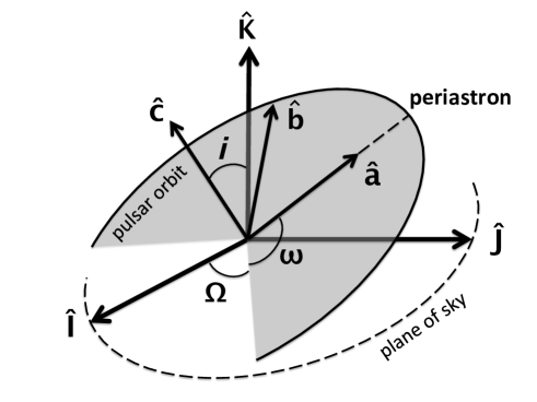
Figure 1: The frame $(\hat{\bf I},\hat{\bf J},\hat{\bf K})$ is comoving with the pulsar system, with $\hat{\bf K}$ pointing along the line of sight to the pulsar from the Earth, while $(\hat{\bf I},\hat{\bf J})$ constitutes the sky plane with $\hat{\bf I}$ to east and $\hat{\bf J}$ to north. The spatial frame $(\hat{\bf a},\hat{\bf b},\hat{\bf c})$ is centered at the pulsar system with $\hat{\bf a}$ pointing from the center of mass to the periastron, $\hat{\bf c}$ along the orbital angular momentum, and $\hat{\bf b}\equiv\hat{\bf c}\times\hat{\bf a}$. The frames, $(\hat{\bf I},\hat{\bf J},\hat{\bf K})$ and $(\hat{\bf a},\hat{\bf b},\hat{\bf c})$, are related through rotation matrices, ${\cal R}^{(\Omega)}$, ${\cal R}^{(i)}$, and ${\cal R}^{(\omega)}$.

In Newtonian gravity, a bound orbit of a binary is a Keplerian ellipse. For a binary pulsar, the shape of the pulsar orbit is specified by the semimajor axis, $a$, and the eccentricity, $e$. The orientation of the orbit with respect to observers is described by three Euler angles, namely the orbital inclination angle, $i$, the longitude of periastron, $\omega$, and the longitude of ascending node, $\Omega$ (see Figure 1 for a graphical illustration). Kepler’s third law relates the orbital size with the orbital period, $P_{b}$, through

$$GM\propto\left(\frac{2\pi}{P_{b}}\right)^{2}a^{3}\,,$$ (3)

where $M\equiv m_{1}+m_{2}$ is the total mass of the system (here we identify $m_{1}$ as the pulsar mass and $m_{2}$ as the companion mass). We further define the orbital frequency, $n_{b}\equiv 2\pi/P_{b}$, the projected semimajor axis of the pulsar orbit, $x\equiv a\sin i$, and the “characteristic” orbital velocity, ${\cal V}_{\rm O}\equiv(GMn_{b})^{1/3}$ for later notation simplification.

In presence of Lorentz-violating fossil fields, the orbital dynamics of a binary pulsar is modified Bailey and Kostelecký (2006); Shao (2014). By using the technique of osculating elements, Bailey and Kostelecký obtained the secular changes for orbital elements after averaging over one orbital period Bailey and Kostelecký (2006),

$$\left\langle\frac{{\rm d}e}{{\rm d}t}\right\rangle = n_{b}F_{e}\sqrt{1-e^{2}}\left(-eF_{e}\bar{s}^{ab}+2\delta X\,{\cal V}_{\rm O}\bar{s}^{0a}\right)\,,$$ (4)

$$\left\langle\frac{{\rm d}\omega}{{\rm d}t}\right\rangle = \frac{3n_{b}{\cal V}_{\rm O}^{2}}{1-e^{2}}-\frac{n_{b}F_{e}\cot i}{\sqrt{1-e^{2}}}\times$$

$$\left(\sin\omega\,\bar{s}^{ac}+\sqrt{1-e^{2}}\cos\omega\,\bar{s}^{bc}+2\delta X\,e{\cal V}_{\rm O}\cos\omega\,\bar{s}^{0c}\right)$$

$$+n_{b}F_{e}\left(F_{e}\frac{\bar{s}^{aa}-\bar{s}^{bb}}{2}+\frac{2}{e}\delta X\,{\cal V}_{\rm O}\bar{s}^{0b}\right)\,,$$

$$\left\langle\frac{{\rm d}x}{{\rm d}t}\right\rangle = \frac{1-\delta X}{2}\frac{F_{e}{\cal V}_{\rm O}\cos i}{\sqrt{1-e^{2}}}\times$$

$$\left(\cos\omega\,\bar{s}^{ac}-\sqrt{1-e^{2}}\sin\omega\,\bar{s}^{bc}-2\delta X\,e{\cal V}_{\rm O}\sin\omega\,\bar{s}^{0c}\right)\,,$$

where we have defined,

$$F_{e} \equiv \frac{1}{1+\sqrt{1-e^{2}}}\,,$$ (7)

$$\delta X \equiv \frac{m_{1}-m_{2}}{m_{1}+m_{2}}\,.$$ (8)

The $\bar{s}^{\mu\nu}$ fields in Eqs. (4–II) are defined in the frame that is comoving with the center of the binary pulsar. The components of $\bar{s}^{\mu\nu}$ are projected onto the spatial coordinate frame $(\hat{\bf a},\hat{\bf b},\hat{\bf c})$ that is attached with the orbit (see Figure 1). The transformation between the pulsar frame and the canonical Sun-centered celestial-equatorial frame is discussed in section III.

We will deal with small-eccentricity NS-WD binaries, where in most cases, the orbits are almost perfectly circular due to mutual tide forces, frictional dissipation, and exchange of materials during the evolutionary history Lorimer and Kramer (2004). Therefore, instead of $e$ and $\omega$, two Laplace-Lagrange parameters, $\eta\equiv e\sin\omega$ and $\kappa\equiv e\cos\omega$, are widely used in practice in order to break the notorious parameter degeneracies Lange et al. (2001). In the limit of $e\ll 1$, it is easy to obtain Shao (2014),

$$\left\langle\frac{{\rm d}e}{{\rm d}t}\right\rangle \simeq n_{b}\delta X\,{\cal V}_{\rm O}\bar{s}^{0a}\,,$$ (9)

$$\left\langle\frac{{\rm d}\omega}{{\rm d}t}\right\rangle \simeq 3n_{b}{\cal V}_{\rm O}^{2}+\frac{n_{b}}{e}\delta X\,{\cal V}_{\rm O}\bar{s}^{0b}\,,$$ (10)

$$\left\langle\frac{{\rm d}x}{{\rm d}t}\right\rangle \simeq \frac{1-\delta X}{4}{\cal V}_{\rm O}\cos i\left(\bar{s}^{ac}\cos\omega-\bar{s}^{bc}\sin\omega\right)\,,$$ (11)

and

$$\left\langle\frac{{\rm d}\eta}{{\rm d}t}\right\rangle \simeq n_{b}\delta X{\cal V}_{\rm O}\left(\bar{s}^{0a}\sin\omega+\bar{s}^{0b}\cos\omega\right)$$ (12)

$$+3en_{b}{\cal V}_{\rm O}^{2}\cos\omega\,,$$

$$\left\langle\frac{{\rm d}\kappa}{{\rm d}t}\right\rangle \simeq n_{b}\delta X{\cal V}_{\rm O}\left(\bar{s}^{0a}\cos\omega-\bar{s}^{0b}\sin\omega\right)$$ (13)

$$-3en_{b}{\cal V}_{\rm O}^{2}\sin\omega\,.$$

These formulae will be used in section IV to construct corresponding tests of gravity.

III Coordinate transformation

In SME, in order to be compatible with the Riemann-Cartan spacetime, the Lorentz symmetry breaking is spontaneous with underlying dynamical fluctuations Kostelecký (2004). With this mechanism, the tensorial background, $\bar{s}^{\mu\nu}$, is observer Lorentz-invariant, while particle Lorentz-violating. Therefore, to experimentally probe the magnitudes of $\bar{s}^{\mu\nu}$ components, an explicit observer coordinate system should be specified. We adopt the standard Sun-centered celestial-equatorial frame, $(\hat{\bf T},\hat{\bf X},\hat{\bf Y},\hat{\bf Z})$, in the experimental studies of SME Bailey and Kostelecký (2006). In the context of post-Newtonian gravity, it is chosen as an asymptotically inertial frame that is comoving with the rest frame of the Solar system and that coincides with the canonical Sun-centered frame. The $\hat{\bf X}$ axis is pointing from the Earth to the Sun at vernal equinox of J2000.0 epoch, and the $\hat{\bf Z}$ axis is along the rotating axis of the Earth, and $\hat{\bf Y}\equiv\hat{\bf Z}\times\hat{\bf X}$ completes a right-handed coordinate system.

For the purpose of this paper, we will assume the existence of a PF for simplicity. The PF can be singled out by the global cosmological evolution or the Universal matter distribution Will and Nordtvedt (1972); Nordtvedt and Will (1972); Will (2014). We will keep the choice of PF general. However, the isotropic CMB frame, which is the most natural choice from the cosmic viewpoint, is kept in mind as a benchmark. This simplification, compared with the most generic case of possible anisotropy in all frames Bailey and Kostelecký (2006); Shao (2014), is discussed in section V.

In the PF, by virtue of rotational invariance, the $s^{\mu\nu}$ tensor takes a simple isotropic form Bailey and Kostelecký (2006),

$$\bar{s}^{\mu\nu}_{\rm PF}=\bar{s}^{00}_{\rm PF}\left(\begin{array}[]{cccc}1&0&0&0\\ 0&\frac{1}{3}&0&0\\ 0&0&\frac{1}{3}&0\\ 0&0&0&\frac{1}{3}\\ \end{array}\right)\,.$$ (14)

Here for numerical reasons, we have denoted $\bar{s}^{00}_{\rm PF}$ to be the $\bar{s}^{00}$ component in the PF. Although the $\bar{s}^{00}$ component of $\bar{s}^{\mu\nu}$ will in general change under a coordinate transformation, the value of $\bar{s}^{00}_{\rm PF}$, which specified in the PF, is fixed. Worthy to mention that, we also naturally have $\bar{t}^{\kappa\lambda\mu\nu}=0$ in the PF Bailey and Kostelecký (2006).

If we consider a frame that is moving with respect to the PF with a velocity ${\bf w}\equiv(w_{\rm X},w_{\rm Y},w_{\rm Z})$, the $s^{\mu\nu}$ matrix takes the form (see Eq. (68) in Ref. Bailey and Kostelecký (2006)),

$$\bar{s}^{\mu\nu}=\bar{s}^{\mu\nu}_{\rm PF}+\bar{s}^{\mu\nu}_{\bf w}\,,$$ (15)

where

$$\bar{s}^{\mu\nu}_{\bf w}=\frac{4}{3}\bar{s}^{00}_{\rm PF}\left(\begin{array}[]{cccc}w_{\rm X}^{2}+w_{\rm Y}^{2}+w_{\rm Z}^{2}&-w_{\rm X}&-w_{\rm Y}&-w_{\rm Z}\\ -w_{\rm X}&w_{\rm X}^{2}&w_{\rm X}w_{\rm Y}&w_{\rm X}w_{\rm Z}\\ -w_{\rm Y}&w_{\rm X}w_{\rm Y}&w_{\rm Y}^{2}&w_{\rm Y}w_{\rm Z}\\ -w_{\rm Z}&w_{\rm X}w_{\rm Z}&w_{\rm Y}w_{\rm Z}&w_{\rm Z}^{2}\\ \end{array}\right)\,.$$ (16)

Previous tests of the pure-gravity sector of SME with pulsar observations, no matter with the orbital dynamics of binary pulsars Bailey and Kostelecký (2006); Shao and Wex (2012); Shao (2014) or the spin evolution of solitary pulsars Shao et al. (2013); Shao (2014), include no observable effect from the component $\bar{s}^{00}\equiv\bar{s}^{11}+\bar{s}^{22}+\bar{s}^{33}$, under the assumption that the Lorentz boost in Eq. (15) is negligible Bailey and Kostelecký (2006). Therefore, we were only able to constrain the other eight time-spatial and spatial-spatial components of $\bar{s}^{\mu\nu}$, even with over-abounded twenty-seven independent tests in Ref. Shao (2014). Nevertheless, with the Lorentz boost, one can clearly see a mixture between the $\bar{s}^{00}$ component and the $\bar{s}^{0j}$ and $\bar{s}^{jk}$ components ($j,k=1,2,3$). Although the systematic velocity of a binary pulsar is small (typically, $|{\bf w}|\sim{\cal O}(10^{-3})$), precision experiments with pulsars can still put a meaningful constraint on the $\bar{s}^{00}$ component with careful studies Shao (2014). This is the main idea of this work that establishes the basis of the test below.

It is worthy to mention that, in the standard post-Newtonian frame of SME, we are interested in constraining the component $\bar{s}^{\rm TT}$, which is the $00$-component of $\bar{s}^{\mu\nu}$ in the standard Sun-centered celestial-equatorial frame, that is

$$\bar{s}^{\rm TT}=\bar{s}^{00}_{\rm PF}\left(1+\frac{4}{3}{\bf w}_{\odot}^{2}\right)\,,$$ (17)

where ${\bf w}_{\odot}$ is the velocity of the Solar system with respect to the PF. This rescaling is negligible, nevertheless, it is accounted for in our calculations.

Besides the boost in Eq. (15), one also needs to perform a spatial rotation, ${\cal R}$, to align the spatial axes of $(\hat{\bf a},\hat{\bf b},\hat{\bf c})$ and $(\hat{\bf X},\hat{\bf Y},\hat{\bf Z})$,

$$\left(\begin{array}[]{c}\hat{\bf a}\\ \hat{\bf b}\\ \hat{\bf c}\end{array}\right)={\cal R}\left(\begin{array}[]{c}\hat{\bf X}\\ \hat{\bf Y}\\ \hat{\bf Z}\end{array}\right)\,.$$ (18)

With the help of an intermediate coordinate system $(\hat{\bf I},\hat{\bf J},\hat{\bf K})$ in Figure 1, one can decompose the full rotation into five simple parts Shao (2014),

$${\cal R}={\cal R}^{(\omega)}{\cal R}^{(i)}{\cal R}^{(\Omega)}{\cal R}^{(\delta)}{\cal R}^{(\alpha)}\,,$$ (19)

with

$${\cal R}^{(\alpha)} = \left(\begin{array}[]{ccc}-\sin\alpha&\cos\alpha&0\\ -\cos\alpha&-\sin\alpha&0\\ 0&0&1\end{array}\right)\,,$$ (23)

$${\cal R}^{(\delta)} = \left(\begin{array}[]{ccc}1&0&0\\ 0&\sin\delta&\cos\delta\\ 0&-\cos\delta&\sin\delta\end{array}\right)\,,$$ (27)

$${\cal R}^{(\Omega)} = \left(\begin{array}[]{ccc}\cos\Omega&\sin\Omega&0\\ -\sin\Omega&\cos\Omega&0\\ 0&0&1\end{array}\right)\,,$$ (31)

$${\cal R}^{(i)} = \left(\begin{array}[]{ccc}1&0&0\\ 0&\cos i&\sin i\\ 0&-\sin i&\cos i\end{array}\right)\,,$$ (35)

$${\cal R}^{(\omega)} = \left(\begin{array}[]{ccc}\cos\omega&\sin\omega&0\\ -\sin\omega&\cos\omega&0\\ 0&0&1\end{array}\right)\,,$$ (39)

where $\alpha$ and $\delta$ are the right ascension and declination of the binary pulsar.

Instead of performing such a rotation to $\bar{s}^{\mu\nu}$ in Eq. (15) or $\bar{s}^{\mu\nu}_{\bf w}$ in Eq. (16), one can decompose the velocity ${\bf w}$ in the $(\hat{\bf a},\hat{\bf b},\hat{\bf c})$ coordinate frame,

$${\bf w} = w_{\rm X}\hat{\bf X}+w_{\rm Y}\hat{\bf Y}+w_{\rm Z}\hat{\bf Z}$$ (40)

$$= w_{a}\hat{\bf a}+w_{b}\hat{\bf b}+w_{c}\hat{\bf c}\,,$$

and replace $(w_{\rm X},w_{\rm Y},w_{\rm Z})$ with $(w_{a},w_{b},w_{c})$ in Eq. (16) to obtain the desired form of $\bar{s}^{\mu\nu}$ in the comoving frame of the pulsar system with the spatial axes $(\hat{\bf a},\hat{\bf b},\hat{\bf c})$. To be more explicit, the components of the $\bar{s}^{\mu\nu}$ field that are to be used in Eqs. (4–13) are Bailey and Kostelecký (2006),

$$\bar{s}^{0a} = -\frac{4}{3}\bar{s}^{00}_{\rm PF}w_{a}\,,$$ (41)

$$\bar{s}^{0b} = -\frac{4}{3}\bar{s}^{00}_{\rm PF}w_{b}\,,$$ (42)

$$\bar{s}^{0c} = -\frac{4}{3}\bar{s}^{00}_{\rm PF}w_{c}\,,$$ (43)

$$\bar{s}^{ab} = \frac{4}{3}\bar{s}^{00}_{\rm PF}w_{a}w_{b}\,,$$ (44)

$$\bar{s}^{bc} = \frac{4}{3}\bar{s}^{00}_{\rm PF}w_{b}w_{c}\,,$$ (45)

$$\bar{s}^{ac} = \frac{4}{3}\bar{s}^{00}_{\rm PF}w_{a}w_{c}\,,$$ (46)

$$\bar{s}^{aa} = \frac{1}{3}\bar{s}^{00}_{\rm PF}(1+4w_{a}^{2})\,,$$ (47)

$$\bar{s}^{bb} = \frac{1}{3}\bar{s}^{00}_{\rm PF}(1+4w_{b}^{2})\,,$$ (48)

$$\bar{s}^{cc} = \frac{1}{3}\bar{s}^{00}_{\rm PF}(1+4w_{c}^{2})\,,$$ (49)

where, to reiterate, $(w_{a},w_{b},w_{c})$ are the components of the 3-dimensional velocity of the pulsar system with respect to the PF, projected on the coordinate frame $(\hat{\bf a},\hat{\bf b},\hat{\bf c})$.

IV Simulations and Results

Table 1: Relevant quantities of PSRs J1012+5307 Lazaridis et al. (2009), J1738+0333 Freire et al. (2012a), and J0348+0432 Antoniadis et al. (2013) for the test, from radio timing and optical spectroscopy observations. Parenthesized numbers represent the $1$-$\sigma$ uncertainty in the last digits quoted. The listed Laplace-Lagrange parameter, $\eta$, is the intrinsic value, after subtraction of the contribution from the Shapiro delay Lange et al. (2001). For orbital inclination, there is an ambiguity between $i$ and $180^{\circ}-i$; only the value $i<90^{\circ}$ is tabulated.

	PSR J1012+5307	PSR J1738+0333	PSR J0348+0432
Observed Quantities
Observational span, $T_{\rm obs}$ (year)	$\sim 15$ Lazaridis et al. (2009)	$\sim 10$ Freire et al. (2012a)	$\sim 4$ Antoniadis et al. (2013)
Right ascension, $\alpha$ (J2000)	${\rm 10^{h}12^{m}33^{s}.4341010(99)}$	${\rm 17^{h}38^{m}53^{s}.9658386(7)}$	${\rm 03^{h}48^{m}43^{s}.639000(4)}$
Declination, $\delta$ (J2000)	$53^{\circ}07^{\prime}02^{\prime\prime}.60070(13)$	$03^{\circ}33^{\prime}10^{\prime\prime}.86667(3)$	$04^{\circ}32^{\prime}11^{\prime\prime}.4580(2)$
Proper motion in $\alpha$, $\mu_{\alpha}~{}(\textrm{mas\,yr}^{-1})$	2.562(14)	7.037(5)	4.04(16)
Proper motion in $\delta$, $\mu_{\delta}~{}(\textrm{mas\,yr}^{-1})$	$-$25.61(2)	5.073(12)	3.5(6)
Distance, $d$ (kpc)	$0.836(80)$	$1.47(10)$	$2.1(2)$
Radial velocity, $v_{r}$ (km s-1)	$44(8)$	$-42(16)$	$-1(20)$
Spin period, $P$ (ms)	5.255749014115410(15)	5.850095859775683(5)	39.1226569017806(5)
Orbital period, $P_{\rm b}$ (day)	0.60467271355(3)	0.3547907398724(13)	0.102424062722(7)
Projected semimajor axis, $x$ (lt-s)	0.5818172(2)	0.343429130(17)	0.14097938(7)
$\eta\equiv e\sin\omega~{}(10^{-7})$	$-1.4(34)$	$-1.4(11)$	$19(10)$
$\kappa\equiv e\cos\omega~{}(10^{-7})$	$0.6(31)$	$3.1(11)$	$14(10)$
Time derivative of $x$, $\dot{x}~{}(10^{-15}~{}\textrm{s\,s}^{-1})$	2.3(8)	0.7(5)	$\cdots$
Mass ratio, $q\equiv m_{1}/m_{2}$	10.5(5)	8.1(2)	11.70(13)
Companion mass, $m_{2}~{}({\rm M}_{\odot})$	0.16(2)	$0.181^{+0.008}_{-0.007}$	0.172(3)
Pulsar mass, $m_{1}~{}(\textrm{M}_{\odot})$	1.64(22)	$1.46^{+0.06}_{-0.05}$	2.01(4)
$\delta X\equiv(q-1)/(q+1)$	0.826(8)	0.780(5)	0.843(2)
Estimated Quantities
Upper limit of $|\dot{x}|~{}(10^{-15}~{}\textrm{s\,s}^{-1})$	$\cdots$	$\cdots$	1.9
Upper limit of $|\dot{\eta}|$ ($10^{-14}\,{\rm s}^{-1}$)	0.25	0.12	2.7
Upper limit of $|\dot{\kappa}|$ ($10^{-14}\,{\rm s}^{-1}$)	0.23	0.12	2.7
Derived Quantities Based on GR
Orbital inclination, $i$ (deg)	52(4)	32.6(10)	40.2(6)
Advance of periastron, $\dot{\omega}\,({\rm deg\,yr}^{-1})$	0.69(6)	1.57(5)	14.9(2)
Characteristic velocity, $\mathcal{V}_{\rm O}\,({\rm km\,s}^{-1})$	308(13)	355(5)	590(4)

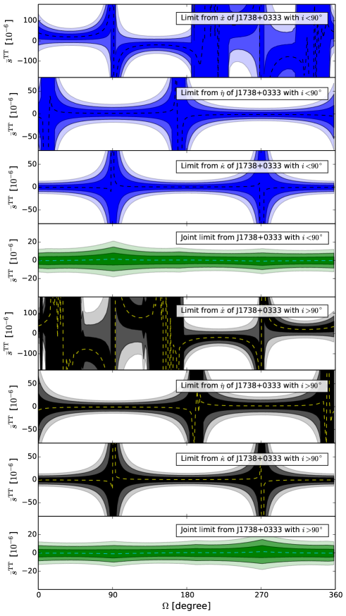
Figure 2: Limits on $\bar{s}^{\rm TT}$ from PSR J1738+0333. In each panel, 1-$\sigma$, 2-$\sigma$, and 3-$\sigma$ contours are drawn with different color scales, while dashed lines are the central values from our Monte Carlo simulations. The upper four panels show in sequence the limits from $\dot{x}$, $\dot{\eta}$, $\dot{\kappa}$ and their combination, with an orbital inclination $i<90^{\circ}$. The cases for $i>90^{\circ}$ are depicted in the lower four panels.

IV.1 Pulsar systems

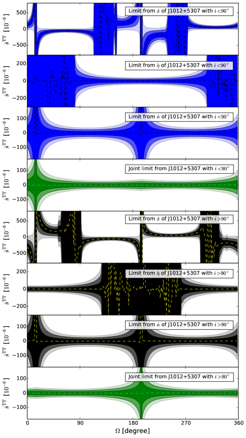
Figure 3: Same as Figure 2, for PSR J1012+5307.

In order to perform tests of the $\bar{s}^{\rm TT}$ component in the pure-gravity sector of SME with binary pulsars, there are several observational requirements that need to be met.

• First of all, because we need the boost to mix different components in the $\bar{s}^{\mu\nu}$ matrix, a measurement of the 3-dimensional velocity of the pulsar system is required. Usually, for a well-timed binary pulsar that is not too far away from the Solar system, we can obtain its proper motion after several years of radio timing. Together with the distance information from the parallax measurement from radio timing, or alternatively, from Very Long Baseline Interferometry (VLBI), we can get the system’s 2-dimensional motion projected on the sky plane. In general, the systematic velocity of the binary along its line of sight is not measurable in radio timing. Fortunately, for some NS-WD systems, we can use the orbitally phase-resolved optical spectroscopy of the white dwarf to separate its sinusoidally varying (projected) orbital velocity and its nearly constant systematic radial velocity Callanan et al. (1998); Antoniadis et al. (2012, 2013). We will make use of three small-eccentricity NS-WD binaries with radial velocity measurements, namely PSRs J1012+5307 Lazaridis et al. (2009), J1738+0333 Freire et al. (2012a) and J0348+0432 Antoniadis et al. (2013).

• As can be seen from Eqs. (4–II), we demand the measurements or upper limits of $\dot{e}$, $\dot{\omega}$ and $\dot{x}$ to perform these tests. Usually, a very good timing precision is needed to achieve these observations. Therefore, only very well timed binary pulsars are considered here (see Table 1). For small-eccentricity binary pulsars, in practice, we use the Laplace-Lagrange parameters, $\eta$ and $\kappa$, to break parameter degeneracies within the fitting procedure of times of arrival of radio pulse signals Lange et al. (2001). Therefore, for these pulsars, we will use $\dot{\eta}$ and $\dot{\kappa}$ in Eqs. (12–13) instead of $\dot{e}$ and $\dot{\omega}$. Because for some pulsars, $\dot{x}$, $\dot{\eta}$, and $\dot{\kappa}$ were not reported along with other timing parameters in their timing solutions published in literature, we adopt the methodology in Ref. Shao (2014). Whenever inaccessible, we conservatively estimate 68% CL upper limits for these parameters as $|\dot{\cal P}|^{\rm upper}=\sqrt{12}\sigma_{\cal P}/T_{\rm obs}$ (${\cal P}=x,\eta,\kappa$), where $T_{\rm obs}$ is the time span used in deriving the timing solution. This choice is in accordance with the case of linear-in-time evolution. It is justified, because if there is any large effect from Lorentz violation or other new sources, the changes in these parameters should have been detected already in these systems, or the uncertainties of $x$, $\eta$, and $\kappa$ derived from times of arrival of pulse signals cannot be too minuscule Shao (2014). Nevertheless, to fully account for all parameter correlations, one will need refitting of times of arrival of these pulsars explicitly with parameters, $\dot{x}$, $\dot{\eta}$, and $\dot{\kappa}$, in the timing model.

• The test of $\bar{s}^{\rm TT}$ is possible only if component masses of the binary are measured independently of the timing parameters we are using in the test. Interestingly, such mass measurements were already obtained, thanks to the optical observations of the WD companions, with the three small-eccentricity binary pulsars we are to use Callanan et al. (1998); Lazaridis et al. (2009); Antoniadis et al. (2012, 2013). From optical observations, the mass of the WD can be inferred based on the WD atmosphere models and, from the ratio of the (projected) orbital velocities of the WD (from optical spectroscopy) and the pulsar (from radio timing), the mass ratio of two components can be derived. Thereby we can get two component masses without assuming GR to be the correct underlying gravity theory as done in other systems with post-Keplerian parameters Stairs (2003); Lorimer and Kramer (2004); Wex (2014). With component masses, one can estimate the mass difference, $\delta X$, and the characteristic orbital velocity of the system, ${\cal V}_{\rm O}$, basing on the Kepler’s third law.

• The geometry of the binary orbit, in terms of three Euler angles, $i$, $\omega$ and $\Omega$, is also required to project the 3-dimensional velocity, ${\bf w}$, onto the coordinate system $(\hat{\bf a},\hat{\bf b},\hat{\bf c})$. The orbital inclination is calculable from Kepler’s law since two masses of the system are known. Because we can only infer $\sin i$ from radio timing, there is an ambiguity between $i$ and $180^{\circ}-i$. The longitude of periastron, $\omega$, is also calculable once $\eta$ and $\kappa$ are given. However, the longitude of ascending node, $\Omega$, is generally not an observable. In Ref. Shao (2014), we had to treat it as an unknown quantity uniformly distributed in the range $[0^{\circ},360^{\circ})$, that renders the tests as probabilistic tests. In this work, we will develop a robust test for $\bar{s}^{\rm TT}$ even without knowing the actual value of $\Omega$. The idea is similar to the robust test of the strong-field parameter, $\hat{\alpha}_{1}$, in the parametrized post-Newtonian (PPN) formalism, in Ref. Shao and Wex (2012), and will be elaborated in detail in the next subsection (also see Ref. Freire et al. (2012b) for a similar idea in testing of strong equivalence principle).

As mentioned, to meet the requirements listed above, we choose PSRs J1012+5307 Lazaridis et al. (2009), J1738+0333 Freire et al. (2012a), and J0348+0432 Antoniadis et al. (2013) to perform the test of $\bar{s}^{\rm TT}$. They are all well-timed small-eccentricity NS-WD binaries with both radio and optical observations. Besides, these binaries are also relativistic binaries with small orbital periods ($P_{b}<15\,$hours). This is important, because relativistic orbits boost the figures of merit of the test with larger orbital frequency, $n_{b}$, and larger characteristic orbital velocity, ${\cal V}_{\rm O}$ (see Eqs. (11–13)). Relevant parameters for the test of these systems, from radio timing and optical spectroscopy, are tabulated in Table 1 (see the original publications Freire et al. (2012a); Lazaridis et al. (2009); Antoniadis et al. (2013) for details).

IV.2 Constraints on $\bar{s}^{\rm TT}$

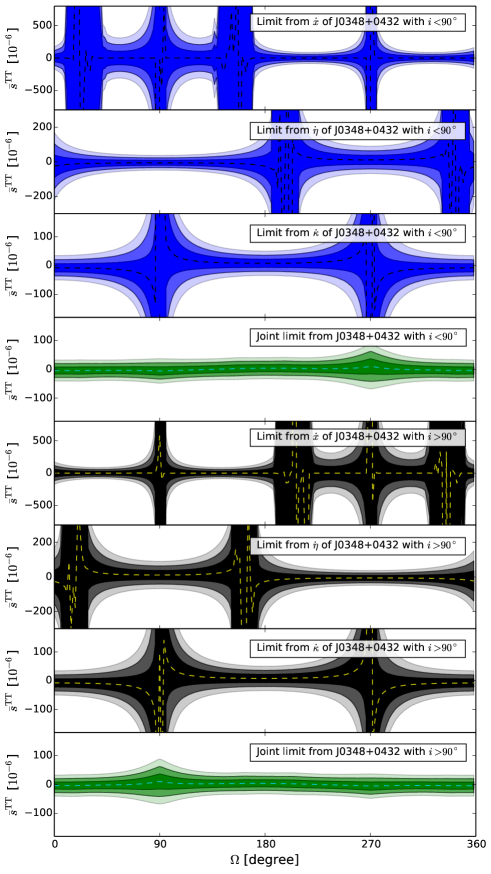
Figure 4: Same as Figure 2, for PSR J0348+0432.

We use expressions of $\dot{x}$, $\dot{\eta}$, and $\dot{\kappa}$ in Eqs. (11–13), together with Eqs. (41–49), to perform tests of $\bar{s}^{\rm TT}$. Here we assume that the isotropic CMB frame singles out a PF (however, see generalized cases in the next section). Therefore, the “absolute” velocity of the pulsar system, ${\bf w}={\bf w}_{\odot}+{\bf v}$, is a vectorial superposition of the velocity of the Solar system to the CMB frame, ${\bf w}_{\odot}$, and the velocity of the pulsar system to the Solar system, ${\bf v}$. From Wilkinson Microwave Anisotropy Probe (WMAP) experiments, a CMB dipole measurement of $3.355\pm 0.008\,$mK was obtained, which implies a peculiar velocity of the Solar system barycentre, $|{\bf w}_{\odot}|=369.0\pm 0.9\,$km s^-1, in the direction of Galactic longitude and latitude, $(l,b)=(263.99^{\circ}\pm 0.14^{\circ},48.26^{\circ}\pm 0.03^{\circ})$ Hinshaw et al. (2013). The 3-dimensional velocities of binary systems, ${\bf v}$’s, are derived from joint radio timing and optical spectroscopy observations. Direct calculations show that the absolute velocities of binary pulsars are of ${\cal O}(10^{-3})$ for three binary systems in Table 1.

Because the longitude of ascending node, $\Omega$, is unknown for all three pulsar systems, we scan through its values in the range $[0^{\circ},360^{\circ})$. After choosing the orbital inclination between $i$ and $180^{\circ}-i$, for each given $\Omega$, we can fix the absolute orientation of the coordinate frame $(\hat{\bf a},\hat{\bf b},\hat{\bf c})$ at Newtonian order. The absolute velocity of the binary is projected on the $(\hat{\bf a},\hat{\bf b},\hat{\bf c})$ frame to get its coordinate components, $(w_{a},w_{b},w_{c})$. Having all these information at hand, from the measured or reasonably estimated $\dot{x}$, $\dot{\eta}$, and $\dot{\kappa}$ (see Table 1), we can calculate limits of $\bar{s}^{\rm TT}$ from Eqs. (11–13) for each $\Omega$.

For each binary pulsar, we perform $10^{5}$ Monte Carlo simulations for each value of $\Omega$ to account for the observational uncertainties in parameters listed in Table 1. From the results of these simulations, we can read out the constraints of $\bar{s}^{\rm TT}$ from $\dot{x}$, $\dot{\eta}$, and $\dot{\kappa}$ separately. The result from PSR J1738+0333 is illustrated in the first three panels of Figure 2 for $\dot{x}$, $\dot{\eta}$, and $\dot{\kappa}$, as a function of $\Omega$ with an orbital inclination $i<90^{\circ}$ (namely, $i=32.6^{\circ}\pm 1.0^{\circ}$). Different colors correspond to 68.3%, 95.5%, and 99.7% CLs. These results remind us the test of the strong-field PPN parameter, $\hat{\alpha}_{2}$, in Ref. Shao and Wex (2012) (see their Figures 2–3), where for some $\Omega$’s, the parameter values are basically unconstrained due to “unfavored” geometrical configurations. This is due to the vectorial/tensorial nature of the LLI violation. It happens for the $\dot{x}$ test in Ref. Shao and Wex (2012), and it is still true for all three tests here (see Ref. Shao and Wex (2012) for more discussions).

For the $\hat{\alpha}_{2}$ test in Ref. Shao and Wex (2012) there is only one “anomalous” parameter entering the test, namely $\dot{x}$, while here we have three parameters entering. Therefore, for a given $\Omega$, if an $\bar{s}^{\rm TT}$ is to pass the test, it should pass all three tests simultaneously. In other words, for a given $\Omega$, we can adopt the tightest constraint of $\bar{s}^{\rm TT}$, out of the three limits from $\dot{x}$, $\dot{\eta}$, and $\dot{\kappa}$. Such limits from PSR J1738+0333 with $i<90^{\circ}$ is depicted in the fourth panel of Figure 2. We can see that, because the unbound situations do not occur simultaneously for all three tests for any given $\Omega$, a quite smooth limit of $\bar{s}^{\rm TT}$ can be attained as a function of $\Omega$. Since there exists no measurement of $\Omega$ for PSR J1738+0333 yet, we conservatively read out the worst constraint from the fourth panel of Figure 2, that gives,

$$|\bar{s}^{\rm TT}|<1.6\times 10^{-5}\quad(95\%~{}{\rm CL})\,,$$ (50)

at $\Omega\simeq 90^{\circ}$.

We also plot the case for $i>90^{\circ}$ (namely, $i=147.4^{\circ}\pm 1.0^{\circ}$) in the last four panels of Figure 2 for PSR J1738+0333. It is symmetric with respect to the case of $i<90^{\circ}$, and the worst limit from the joint constraint (the eighth panel) also gives $|\bar{s}^{\rm TT}|<1.6\times 10^{-5}~{}(95\%~{}{\rm CL})$, at $\Omega\simeq 270^{\circ}$. We claim that this limit is robust instead of probabilistic, in contrast to the limits presented in Ref. Shao (2014) where $\Omega$’s were effectively “averaged” out in the range $[0^{\circ},360^{\circ})$. The limit in Eq. (50) is about 500 times better than the current best (yet unique) limit from the GPB experiment Bailey et al. (2013).

The constraints from PSR J1012+5307 are illustrated in Figure 3 as a function of $\Omega$. In this system, it is seen that for the joint limit, there still exist unconstrained regions for $\bar{s}^{\rm TT}$ around $\Omega\simeq 15^{\circ}$ for $i<90^{\circ}$ (and $\Omega\simeq 195^{\circ}$ for $i>90^{\circ}$). The performance of PSR J1012+5307 is in accordance with its performance in the $\hat{\alpha}_{1}$ test in Ref. Shao and Wex (2012), where PSR J1738+0333 is better in constraining the PF effects in the PPN formalism as well. Partial reason for this performance will be discussed in the next section.

The constraints from PSR J0348+0432 are illustrated in Figure 4 as a function of $\Omega$. The joint limit shows a smooth constraint versus $\Omega\in[0^{\circ},360^{\circ})$, and from its joint constraint, we get the worst limit,

$$|\bar{s}^{\rm TT}|<7.2\times 10^{-5}\quad(95\%~{}{\rm CL})\,,$$ (51)

at $\Omega\simeq 270^{\circ}$ for $i<90^{\circ}$ (and at $\Omega\simeq 90^{\circ}$ for $i>90^{\circ}$). It is about five times weaker than the limit from PSR J1738+0333, yet still 100 times better than the GPB limit.

V Discussions

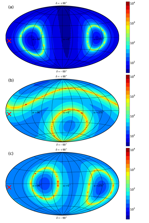
Figure 5: The constraints of $|\bar{s}^{\rm TT}|$ from PSRs J1738+0333 (a), J1012+5307 (b), and J0348+0432 (c) for different PFs. Here $(\alpha,\delta)$ denotes the direction of the absolute motion of the Solar system with respect to a PF. The magnitude of this motion is assumed to be $|{\bf w}_{\odot}|\simeq 369\,{\rm km\,s}^{-1}$. The red cross denotes the direction of the CMB frame, that has equatorial coordinates, $(\alpha,\delta)_{\rm CMB}\simeq(168^{\circ},-7^{\circ})$. Notice that, for convenience in comparison, all three figures use the same color scaling, as displayed on the right side. The unit for $\bar{s}^{\rm TT}$ is $10^{-6}$.

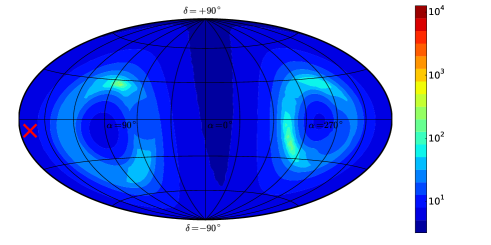
Figure 6: Same as Figure 5, for the combined constraint from three binary pulsars — PSRs J1738+0333, J1012+5307, and J0348+0432. For convenience in comparison, it uses the same color scaling as that of Figure 5. The unit for $\bar{s}^{\rm TT}$ is $10^{-6}$.

While using the isotropic CMB frame as the PF, we are basically assuming that the PF is determined by the global matter distribution in the Universe, and that the extra vectorial or tensorial components of gravitational interaction are of long range, at least comparable to the Hubble radius. When this is generally the most plausible assumption, it is still interesting to consider other PFs, and further show the power of binary pulsars in constraining LLI violation in the gravity sector.

It is straightforward to apply the computations above to other PFs. We here assume that the Solar system is moving with respect to a PF, with a velocity, ${\bf w}_{\odot}$. Its magnitude is assumed to be $|{\bf w}_{\odot}|\simeq 369\,{\rm km\,s}^{-1}$, while its direction is $(\alpha,\delta)$ when expressed in the equatorial coordinate. For every pair of $(\alpha,\delta)$, we perform the test above to get the worst constraint of $\bar{s}^{\rm TT}$ from joint limits of $\dot{x}$, $\dot{\eta}$, and $\dot{\kappa}$, for each pulsar. These limits at 68.3% CL are depicted as contours in Figure 5 for PSRs J1738+0333, J1012+5307, and J0348+0432. For the reason of computational burden, we have ignored the measurement uncertainties of parameters except those of $\dot{x}$, $\dot{\eta}$, and $\dot{\kappa}$ for the illustrated results in the figure. We have checked that this treatment only affects our results at a level $\lesssim 20\%$. We can read out the following results from Figure 5 —

• For each pulsar, there are two cones with opposite directions of ${\bf w}_{\odot}$ that provide almost no constraint on $\bar{s}^{\rm TT}$ for the worst limit versus $\Omega$. This is similar to the PF tests in Ref. Shao and Wex (2012) (see their Figure 8).

• With current timing precision, PSR J1738+0333 has a better power, for most directions of ${\bf w}_{\odot}$, in constraining $\bar{s}^{\rm TT}$ over PSRs J1012+5307 and J0348+0432.

• The CMB frame has a direction $(\alpha,\delta)_{\rm CMB}\simeq(168^{\circ},-7^{\circ})$, denoted as a red cross in Figure 5. Compared with the other two pulsars, it is nearer to the “unconstraining zones” of PSR J1012+5307, hence this pulsar provides a much worse constraint on $\bar{s}^{\rm TT}$ when the CMB frame is assumed to be the PF.

It is interesting to notice that, the “unconstraining zones” of different pulsars are different. Therefore, when combining all constraints from all pulsars can effectively eliminate these “unconstraining zones”. The result of such a combination is shown in Figure 6. It is clearly seen that such a combination indeed eliminates almost all unconstrained directions. The worst directions still provide tight constraints of $|\bar{s}^{\rm TT}|\lesssim{\cal O}(10^{-4})$ at 68.3% CL, where $|{\bf w}_{\odot}|$ is again assumed to be 369 km s^-1. For a different velocity of the Solar system, the constraint of $\bar{s}^{\rm TT}$ can be obtained from our result with a proper rescaling.

Nevertheless, it is dangerous to naively combine limits from different binary pulsars if strong-field effects, associated with NSs, play a significant role. In scalar-tensor theories, Damour and Esposito-Farèse discovered that, within some parameter space, the strong fields associated with NSs can develop nonperturbative gravitational effects which can modify the orbital dynamics significantly. This phenomenon is named as “scalarization” Damour and Esposito-Farese (1993). Although in the Einstein-Æther theory and Hořava-Lifshitz gravity, no similar phenomena were found Yagi et al. (2014), there is no formal proof yet that, for gravity theories with LLI violation, similar strong-field dynamics like “scalarization” is absent in general with compact bodies. Therefore, to be conservative, we claim that the limit of $\bar{s}^{\rm TT}$ obtained in this work should be treated as a strong-field limit to its weak-field counterpart. This statement does not necessarily mean that the limit from binary pulsars is “weak”, on the contrary, in most cases the limits from strongly self-gravitating bodies are much stronger than the corresponding limits from weakly gravitating bodies. For example, the parameter for the strong equivalence principle violation, $\Delta$, obtained from binary pulsars (see e.g. Refs. Stairs (2003); Stairs et al. (2005); Wex (2014)), is in general a factor of ${\cal C}_{\rm NS}/{\cal C}_{0}$ stronger in terms of the Nordtvedt parameter, than a corresponding limit from a weakly gravitating body with compactness ${\cal C}_{0}$. For NSs, we have ${\cal C}_{\rm NS}\sim 0.2$, while for the Earth and the Sun, we have ${\cal C}_{\oplus}\sim 10^{-10}$ and ${\cal C}_{\odot}\sim 10^{-6}$ respectively.

In scalar-tensor theories, if the mentioned scalarization happens, the strong-field parameters of gravity theories, such as the PPN parameters, $\beta$ and $\gamma$, will depend on the compactness of the gravitating body. In other words, they become system dependent. If such phenomenon also happens here, we will expect different values of $\bar{s}^{\rm TT}$ for PSRs J1738+0333, J1012+5307, and J0348+0432. Nonetheless, if the dynamics is still within the perturbative region of the gravity theory, these $\bar{s}^{\rm TT}$’s will be of similar values, and in this situation, we are eligible to combine results from different binary pulsars, as done in Figure 6.

Worthy to reemphasize that the $\bar{s}^{\rm TT}$ constraints here are based on robust designs of tests, in contrast to the probabilistic tests performed in Ref. Shao (2014). The achievement is made possible with multiple observables measured simultaneously. Even without a clear knowledge on $\Omega$, picking the worst limit out of all possible limits makes the test very robust. Such ideas were also proposed in Refs. Freire et al. (2012b); Shao and Wex (2012) under different topics on tests of gravity. In the future if we can measure the longitude of ascending node for these binary pulsars, with e.g. interstellar scintillation rcn+14 , we will gain further in constraining the SME parameters.

In the pure-gravity sector of mSME, there are in total nine degrees of freedom to deviate away from GR at leading order Bailey and Kostelecký (2006). Here to focus on the theme of testing $\bar{s}^{\rm TT}$ and to reduce the burden of work, we have assumed that there exists a PF where the spacetime is isotropic. Universal anisotropy can exist in principle within the framework of SME. Therefore, the actual constraint in this paper could be a linear combination of $\bar{s}^{\rm TT}$ and the other time-spatial and spatial-spatial components of $\bar{s}^{\mu\nu}$. However, it was already shown in Ref. Shao (2014), that the time-spatial and spatial-spatial components of $\bar{s}^{\mu\nu}$ were constrained to very small values at levels of ${\cal O}(10^{-9})$–${\cal O}(10^{-11})$, and more importantly, with multiple pulsar systems with different positions in the sky, different spatial orientations of orbits, and different 3-dimensional systematic velocities, the limits of these components tend to have very little mutual correlations (see Figure 3 in Ref. Shao (2014)). Therefore, the limit obtained in this paper is reliable even when there exists no PF at all for the gravity sector in SME.

From another viewpoint, in the past few years, the time-spatial and spatial-spatial components in the Sun-centered celestial-equatorial frame were already stringently constrained by lunar laser ranging bcs07 , atom interferometry mch+08 ; cch+09 , and radio pulsars Shao (2014). Among these, the current best limits were obtained from the systematic analysis of 27 tests from 13 pulsar systems Shao (2014). From the joint analysis of orbital dynamics of binary pulsars and spin evolution of solitary pulsars, the components of $\bar{s}^{\mu\nu}$ were constrained to be, at 68% confidence level, $\lesssim 10^{-9}$ for $\bar{s}^{\rm TX}$, $\bar{s}^{\rm TY}$, and $\bar{s}^{\rm TZ}$, and $\lesssim 10^{-11}$ for $\bar{s}^{\rm XY}$, $\bar{s}^{\rm YZ}$, $\bar{s}^{\rm XZ}$, $\bar{s}^{\rm XX}-\bar{s}^{\rm YY}$, and $\bar{s}^{\rm XX}+\bar{s}^{\rm YY}-2\bar{s}^{\rm ZZ}$ (see Table 1 in Ref. Shao (2014)). Therefore, we can empirically write the $\bar{s}^{\mu\nu}$ field in the Sun-centered frame as

$$\bar{s}^{\mu\nu}\simeq\left(\begin{array}[]{cccc}\bar{s}^{\rm TT}&0&0&0\\ 0&\frac{1}{3}\bar{s}^{\rm TT}&0&0\\ 0&0&\frac{1}{3}\bar{s}^{\rm TT}&0\\ 0&0&0&\frac{1}{3}\bar{s}^{\rm TT}\\ \end{array}\right)\,.$$ (52)

By writing down the above numerical expression with possibly dominant nonzero components from purely empirical evidence bcs07 ; mch+08 ; cch+09 ; Shao (2014), we are free of assuming the existence of a PF. The calculation to constrain such an $\bar{s}^{\mu\nu}$ is straightforward with the analysis in this paper. With Monte Carlo simulations properly accounting for all measurement uncertainties, we found that the best robust limit of $\bar{s}^{\rm TT}$ still comes from PSR J1738+0333, that gives

$$|\bar{s}^{\rm TT}|<2.8\times 10^{-4}\quad(95\%~{}{\rm CL})\,.$$ (53)

It is weaker than the limit with the isotropic frame of CMB as the PF, due to the fact that the boost between PSR J1738+0333 and the Solar system is only about $|{\bf v}|=74.8\pm 9.5\,{\rm km\,s}^{-1}$. The systematic velocity is related to the evolutionary history of NS-WD systems Lorimer and Kramer (2004). Nevertheless, this limit, free of the assumption that there exists a PF, is still one order of magnitude better than the current best limit.

VI Summary

In this paper, we propose a new idea to test the $\bar{s}^{\rm TT}$ component in the pure-gravity sector of mSME by utilizing the boost between different frames. A new robust limit, in the standard Sun-centered equatorial-celestial coordinate frame, is obtained from PSR J1738+0333,

$$|\bar{s}^{\rm TT}|<1.6\times 10^{-5}\quad(95\%~{}{\rm CL})\,,$$ (54)

when the isotropic CMB frame is assumed to be the PF. The limit is about 500 times better than the current best limit from Gravity Probe B Bailey et al. (2013).

The idea of mixing different components in the condensed (cosmic or even local) tensor fields with a full Lorentz transformation is also applicable in other sectors of SME with careful studies, as demonstrated in Refs. cbp+04 ; hac+08 ; gkv14 . Although such a boost is usually quite small (e.g. ${\cal O}(10^{-3})$ for binary pulsars), with some astrophysical systems, the method could become useful with precision experiments, as done here with the state-of-the-art pulsar timing experiments.

References

- Misner et al. (1973) C. W. Misner, K. S. Thorne, and J. A. Wheeler, Gravitation (San Francisco: W.H. Freeman and Company, 1973).
- Will (2014) C. M. Will, Living Reviews in Relativity 17, 4 (2014), eprint arXiv:1403.7377.
- Einstein (1916) A. Einstein, Annalen der Physik 354, 769 (1916).
- Shapiro (1964) I. I. Shapiro, Physical Review Letters 13, 789 (1964).
- Matthews and Sandage (1963) T. A. Matthews and A. R. Sandage, Astrophys. J. 138, 30 (1963).
- Hewish et al. (1968) A. Hewish, S. J. Bell, J. D. H. Pilkington, P. F. Scott, and R. A. Collins, Nature (London) 217, 709 (1968).
- Penzias and Wilson (1965) A. A. Penzias and R. W. Wilson, Astrophys. J. 142, 419 (1965).
- Everitt et al. (2011) C. W. F. Everitt, D. B. Debra, B. W. Parkinson, J. P. Turneaure, J. W. Conklin, M. I. Heifetz, G. M. Keiser, A. S. Silbergleit, T. Holmes, J. Kolodziejczak, et al., Physical Review Letters 106, 221101 (2011), eprint arXiv:1105.3456.
- Kramer et al. (2006) M. Kramer, I. H. Stairs, R. N. Manchester, M. A. McLaughlin, A. G. Lyne, R. D. Ferdman, M. Burgay, D. R. Lorimer, A. Possenti, N. D’Amico, et al., Science 314, 97 (2006), eprint arXiv:astro-ph/0609417.
- Breton et al. (2008) R. P. Breton, V. M. Kaspi, M. Kramer, M. A. McLaughlin, M. Lyutikov, S. M. Ransom, I. H. Stairs, R. D. Ferdman, F. Camilo, and A. Possenti, Science 321, 104 (2008), eprint arXiv:0807.2644.
- Sathyaprakash and Schutz (2009) B. S. Sathyaprakash and B. F. Schutz, Living Reviews in Relativity 12, 2 (2009), eprint arXiv:0903.0338.
- Pitkin et al. (2011) M. Pitkin, S. Reid, S. Rowan, and J. Hough, Living Reviews in Relativity 14, 5 (2011), eprint arXiv:1102.3355.
- Gair et al. (2013) J. R. Gair, M. Vallisneri, S. L. Larson, and J. G. Baker, Living Reviews in Relativity 16, 7 (2013), eprint arXiv:1212.5575.
- Hobbs (2013) G. Hobbs, Classical and Quantum Gravity 30, 224007 (2013), eprint arXiv:1307.2629.
- Kramer and Champion (2013) M. Kramer and D. J. Champion, Classical and Quantum Gravity 30, 224009 (2013).
- McLaughlin (2013) M. A. McLaughlin, Classical and Quantum Gravity 30, 224008 (2013), eprint arXiv:1310.0758.
- Yunes and Siemens (2013) N. Yunes and X. Siemens, Living Reviews in Relativity 16, 9 (2013), eprint arXiv:1304.3473.
- Capozziello and de Laurentis (2011) S. Capozziello and M. de Laurentis, Phys. Rep. 509, 167 (2011), eprint arXiv:1108.6266.
- Clifton et al. (2012) T. Clifton, P. G. Ferreira, A. Padilla, and C. Skordis, Phys. Rep. 513, 1 (2012), eprint arXiv:1106.2476.
- Ashby (2003) N. Ashby, Living Reviews in Relativity 6, 1 (2003).
- Abramowicz and Fragile (2013) M. A. Abramowicz and P. C. Fragile, Living Reviews in Relativity 16, 1 (2013), eprint arXiv:1104.5499.
- Hořava (2009) P. Hořava, Phys. Rev. D 79, 084008 (2009), eprint arXiv:0901.3775.
- Jacobson and Mattingly (2001) T. Jacobson and D. Mattingly, Phys. Rev. D 64, 024028 (2001), eprint arXiv:gr-qc/0007031.
- Bailey and Kostelecký (2006) Q. G. Bailey and V. A. Kostelecký, Phys. Rev. D 74, 045001 (2006), eprint arXiv:gr-qc/0603030.
- Bailey et al. (2013) Q. G. Bailey, R. D. Everett, and J. M. Overduin, Phys. Rev. D 88, 102001 (2013), eprint arXiv:1309.6399.
- Shao (2014) L. Shao, Physical Review Letters 112, 111103 (2014), eprint arXiv:1402.6452.
- Kostelecký and Samuel (1989a) V. A. Kostelecký and S. Samuel, Phys. Rev. D 39, 683 (1989a).
- Kostelecký and Samuel (1989b) V. A. Kostelecký and S. Samuel, Phys. Rev. D 40, 1886 (1989b).
- Colladay and Kostelecký (1997) D. Colladay and V. A. Kostelecký, Phys. Rev. D 55, 6760 (1997), eprint arXiv:hep-ph/9703464.
- Colladay and Kostelecký (1998) D. Colladay and V. A. Kostelecký, Phys. Rev. D 58, 116002 (1998), eprint arXiv:hep-ph/9809521.
- (31) O. Nachtmann, Conf. Proc. C 690224, 485 (1969).
- (32) S. Chadha and H. B. Nielsen, Nucl. Phys. B 217, 125 (1983).
- (33) F. R. Klinkhamer, Nucl. Phys. B 578, 277 (2000) [arXiv:hep-th/9912169].
- Kostelecký and Russell (2011) V. A. Kostelecký and N. Russell, Reviews of Modern Physics 83, 11 (2011), eprint arXiv:0801.0287.
- Kostelecký (2004) V. A. Kostelecký, Phys. Rev. D 69, 105009 (2004), eprint arXiv:hep-th/0312310.
- (36) Q. G. Bailey, V. A. Kostelecký, and R. Xu, arXiv:1410.6162.
- Kostelecký and Tasson (2011) V. A. Kostelecký and J. D. Tasson, Phys. Rev. D 83, 016013 (2011), eprint arXiv:1006.4106.
- Higgs (2014) P. W. Higgs, Rev. Mod. Phys. 86, 851 (2014).
- Englert (2014) F. Englert, Rev. Mod. Phys. 86, 843 (2014).
- Lorimer and Kramer (2004) D. R. Lorimer and M. Kramer, Handbook of Pulsar Astronomy (Cambridge University Press, 2004).
- Lange et al. (2001) C. Lange, F. Camilo, N. Wex, M. Kramer, D. C. Backer, A. G. Lyne, and O. Doroshenko, MNRAS 326, 274 (2001), eprint arXiv:astro-ph/0102309.
- Will and Nordtvedt (1972) C. M. Will and K. Nordtvedt, Jr., Astrophys. J. 177, 757 (1972).
- Nordtvedt and Will (1972) K. Nordtvedt, Jr. and C. M. Will, Astrophys. J. 177, 775 (1972).
- Shao and Wex (2012) L. Shao and N. Wex, Classical and Quantum Gravity 29, 215018 (2012), eprint arXiv:1209.4503.
- Shao et al. (2013) L. Shao, R. N. Caballero, M. Kramer, N. Wex, D. J. Champion, and A. Jessner, Classical and Quantum Gravity 30, 165019 (2013), eprint arXiv:1307.2552.
- Lazaridis et al. (2009) K. Lazaridis, N. Wex, A. Jessner, M. Kramer, B. W. Stappers, G. H. Janssen, G. Desvignes, M. B. Purver, I. Cognard, G. Theureau, et al., MNRAS 400, 805 (2009), eprint arXiv:0908.0285.
- Freire et al. (2012a) P. C. C. Freire, N. Wex, G. Esposito-Farèse, J. P. W. Verbiest, M. Bailes, B. A. Jacoby, M. Kramer, I. H. Stairs, J. Antoniadis, and G. H. Janssen, MNRAS 423, 3328 (2012a), eprint arXiv:1205.1450.
- Antoniadis et al. (2013) J. Antoniadis, P. C. C. Freire, N. Wex, T. M. Tauris, R. S. Lynch, M. H. van Kerkwijk, M. Kramer, C. Bassa, V. S. Dhillon, T. Driebe, et al., Science 340, 448 (2013), eprint arXiv:1304.6875.
- Callanan et al. (1998) P. J. Callanan, P. M. Garnavich, and D. Koester, MNRAS 298, 207 (1998).
- Antoniadis et al. (2012) J. Antoniadis, M. H. van Kerkwijk, D. Koester, P. C. C. Freire, N. Wex, T. M. Tauris, M. Kramer, and C. G. Bassa, MNRAS 423, 3316 (2012), eprint arXiv:1204.3948.
- Stairs (2003) I. H. Stairs, Living Reviews in Relativity 6, 5 (2003), eprint arXiv:astro-ph/0307536.
- Wex (2014) N. Wex, arXiv:1402.5594.
- Kramer and Wex (2009) M. Kramer and N. Wex, Classical and Quantum Gravity 26, 073001 (2009).
- Freire et al. (2012b) P. C. C. Freire, M. Kramer, and N. Wex, Classical and Quantum Gravity 29, 184007 (2012b), eprint arXiv:1205.3751.
- Hinshaw et al. (2013) G. Hinshaw, D. Larson, E. Komatsu, D. N. Spergel, C. L. Bennett, J. Dunkley, M. R. Nolta, M. Halpern, R. S. Hill, N. Odegard, et al., ApJS 208, 19 (2013), eprint arXiv:1212.5226.
- Damour and Esposito-Farese (1993) T. Damour and G. Esposito-Farèse, Physical Review Letters 70, 2220 (1993).
- Yagi et al. (2014) K. Yagi, D. Blas, E. Barausse, and N. Yunes, Phys. Rev. D 89, 084067 (2014), eprint arXiv:1311.7144.
- Stairs et al. (2005) I. H. Stairs, A. J. Faulkner, A. G. Lyne, M. Kramer, D. R. Lorimer, M. A. McLaughlin, R. N. Manchester, G. B. Hobbs, F. Camilo, A. Possenti, et al., Astrophys. J. 632, 1060 (2005), eprint arXiv:astro-ph/0506188.
- (59) B. J. Rickett, W. A. Coles, C. F. Nava, M. A. McLaughlin, S. M. Ransom, F. Camilo, R. D. Ferdman, P. C. C. Freire, M. Kramer, A. G. Lyne, and I. H. Stairs, Astrophys. J. 787, 161 (2014), arXiv:1404.1120.
- (60) J. B. R. Battat, J. F. Chandler, and C. W. Stubbs, Physical Review Letters 99, 241103 (2007), arXiv:0710.0702.
- (61) H. Müller, S.-W. Chiow, S. Herrmann, S. Chu, and K.-Y. Chung, Physical Review Letters 100, 031101 (2008), arXiv:0710.3768.
- (62) K.-Y. Chung, S.-W. Chiow, S. Herrmann, S. Chu, and H. Müller, Phys. Rev. D 80, 016002 (2009), arXiv:0905.1929.
- (63) F. Canè, D. Bear, D. F. Phillips, M. S. Rosen, C. L. Smallwood, R. E. Stoner, R. L. Walsworth, and V. A. Kostelecký, Physical Review Letters 93, 230801 (2004), arXiv:physics/0309070.
- (64) B. R. Heckel, E. G. Adelberger, C. E. Cramer, T. S. Cook, S. Schlamminger, and U. Schmidt, Phys. Rev. D 78, 092006 (2008), arXiv:0808.2673.
- (65) A. H. Gomes, V. A. Kostelecký, and A. J. Vargas, Phys. Rev. D 90, 076009 (2014), arXiv:1407.7748.