End-to-End Reliability-Aware Scheduling for Wireless Sensor Networks

Abstract

Wireless Sensor Networks (WSN) are gaining popularity as a flexible and economical alternative to field-bus installations for monitoring and control applications. For mission-critical applications, communication networks must provide end-to-end reliability guarantees, posing substantial challenges for WSN. Reliability can be improved by redundancy, and is often addressed on the MAC layer by re-submission of lost packets, usually applying slotted scheduling. Recently, researchers have proposed a strategy to optimally improve the reliability of a given schedule by repeating the most rewarding slots in a schedule incrementally until a deadline. This Incrementer can be used with most scheduling algorithms but has scalability issues which narrows its usability to offline calculations of schedules, for networks that are rather static. In this paper, we introduce SchedEx, a generic heuristic scheduling algorithm extension which guarantees a user-defined end-to-end reliability. SchedEx produces competitive schedules to the existing approach, and it does that consistently more than an order of magnitude faster. The harsher the end-to-end reliability demand of the network, the better SchedEx performs compared to the Incrementer. We further show that SchedEx has a more evenly distributed improvement impact on the scheduling algorithms, whereas the Incrementer favors schedules created by certain scheduling algorithms.

I Introduction

Wireless has been promoted as a flexible alternative to wired field-bus, and is therefore pushing forward into the industrial market [1], thereby widening the scope from more basic information harvesting (sensing) applications for the offline analysis of data, to receiving more and more responsibility for control (acting). The challenge with wireless networks is that they use a communication medium which is intrinsically open and vulnerable to interference, so that the medium access control (MAC) plays a vital role for the guarantee of end-to-end qualities [2]. The two industrial wireless standards that stand for the largest market share, WirelessHART in the first place, and ISA 100.11a in the second place, follow a centralized approach with a central network manager, responsible for the scheduling configuration. WirelessHART adopts the IEEE 802.15.4 PHY layer and the MAC needs to conform to the IEEE 802.15.4 standard. To increase the reliability, WirelessHART uses time-division multiple access (TDMA) and automatic repeat-reQuest (ARQ), but leaves much of the scheduling algorithm specifics and implementation to the vendor. Contention-free protocols are preferred over contention-based protocols, such as carrier sense multiple access (CSMA), because packet delivery is more predictable and energy can easier be saved (e.g. by duty-cycling) [4, 5].

Much of the MAC-layer scheduling research that has been conducted assumes in the network model that packet delivery is certain [6], [7]. The main challenge under that assumption is to identify as short a conflict-free schedule frame as possible that allows all sensors to transmit their packets to a set of sinks or gateways with direct and reliable connections to the network manager. With harsh network-wide delay and reliability constraints, the difficulty of the scheduling problems to be solved increases drastically, and the review of the state-of-the-art declares the combined end-to-end guarantee of quality of service (QoS) features such as reliability and delay as open research [2].

In communication systems, end-to-end reliability is commonly defined as the end-to-end probability that all transmitted packets arrive at their destination before a common deadline has been reached, or before several individual deadlines have been reached. For many industrial applications reliability guarantees are a fixed constraint. A latency bound is of no value if it does not hold at a certain reliability level and lost packets or missed deadlines imply severe consequences for many industrial control applications. Scheduling algorithms in the literature lack the ability of reliability guarantees in the schedule creation process [6, 8]. An improvement of reliability can be achieved by means of redundancy. Redundancy can be implemented on different layers, and come in the form of, e.g., redundant packet content and error correction codes (physical layer), repeated transmissions (MAC layer), the installation of relays to improve connectivity, or the concurrent transmission of packets over multiple paths. Every reliability improving means has it’s caveat, including increased costs, maintenance efforts, or packet delay.

In this paper, we improve reliability on the MAC layer by means of dedicated spare opportunities for packet transmission. The authors in [8] propose a two-step process where initially a schedule is created by one of many scheduling algorithms and then incremented in order to maximize reliability until the maximum acceptable delay has been reached. However, the proposed incremental improvement function is not scalable, and it requires a two-step process; scheduling, and extending. The problem we address is the lack of a scalable, fast to compute and reliability ensuring scheduling algorithm. Running solver software for hours to identify optimal results is not an option for industrial WSN with resource constrained field devices.

We propose SchedEx, a low-complexity generic extension for existing slot-based scheduling algorithms. SchedEx ensures that the resulting schedule frame guarantees a lower end-to-end reliability bound $\underline{\rho}$. SchedEx, as opposed to the Incrementer presented in [8], does not require a valid schedule frame to start with. With SchedEx, schedules can be swiftly calculated at the network manager, or the sensors. The information can be used for a substantially faster re-scheduling than what has been possible thus far. Further, the algorithm could be integrated into cross layer optimization frameworks for re-routing and scheduling. We prove that SchedEx guarantees a user-defined reliability level $\underline{\rho}\in[0,1]$, not increasing the scheduling algorithm complexity by more than a constant factor. The repetition vector it requires for the calculation of necessary repeats is created in $O(|\mathcal{T}|)$, where $\mathcal{T}$ is the amount of transmitters in the network. We compare four recently introduced scheduling algorithms using SchedEx and obtain results that are competitive to the method in [8] for harsh reliability requirements, doing that an order of magnitude faster. We apply single-path routing with a fixed set of transmitters and a single sink, in order to make our results comparable to existing work in [8]. However, without loss of generality, SchedEx can be applied to topologies with arbitrary flows and/or multi-path routing.

The remainder of the paper is organized as follows. Section II gives an overview of related work, Section III provides the network model and general assumptions. Section IV explains the approach, specifying the investigated topologies, and introducing SchedEx. The simulations with their results are presented in Section V. The paper concludes with a discussion in VI and concluding remarks in VII.

II Related Work

Various scheduling problem variants have been investigated in the literature (e.g. [6, 7, 9, 10]). The decision making with respect to medium access and routing have a dominating influence on the QoS. The medium access in proposals for mission-critical applications have been dominated by the TDMA approach [6], also adapted in WirelessHART [11], ISA 100.11a [12], WIA-PA [13], and IEEE 802.15.4e [14]. Using TDMA, sensors require time synchronization, and permissions for transmission are assigned based on dedicated slots in a recurrent TDMA schedule-frame. That way, within-network interference is reduced to a minimum while introducing an administrative overhead. Finding minimal TDMA schedules for a WSN graph is an NP-hard problem [6]. For dynamic environments with conflicts changing over time, the tracking of an optimum becomes computationally infeasible even ignoring interference, packet-loss, and time synchronization in the problem formulation. Fortunately, WSNs for automation do usually not require optimal solutions, but solutions that satisfy QoS constraints with highest possible reliability.

Substantial research for reliability improvement has been conducted in the field of industrial wireless sensor networks (IWSN) [15, 16, 17, 18, 19], which underlines the need for reliability ensuring scheduling. The authors in [2] give a recent review of existing research on QoS guarantees for mission-critical WSN applications. The diversity of applications and their constraints with WSN as a potential solution imply that the tailored proposals in the literature are diverse and problem dependent too, for instance with regards to topology, traffic patterns, or the assignment of responsibilities in the network. Thus, general approaches for guarantees on reliability, latency, and other quality measures (such as jitter, or throughput), considering network dynamics, are highly demanded.

The approaches introduced in [20] and [21] propose offline dimensioning with a-priori assessment of packet delivery ratios on the MAC-layer using TDMA scheduling. Burst-error metrics are used in order to improve end-to-end reliability where latency-bounds are reported by repeating slots until a deadline. The greedy algorithm from [21] employs spatial-reuse to provide latency guarantees, a technique that allows multiple sensors to transmit simultaneously if they are not interfering with one another which can considerably reduce schedule frame sizes, and thereby reduce latency. The underlying packet reception rates for the WSNs in [20, 21] go unreported. They could be high, showing only small traces of interference, which would not be a generalizable assumption for industrial networks [22]. Distributed best-effort protocols like the one in [23] can surely improve on performance in best-effort multi-hop networks, but for the use in industrial networks with harsh end-to-end constraints, best-effort is not enough and centralized solutions are needed.

Recently, researchers have started to consider the trade-off between latency and reliability given it a theoretical basis. A first study on scheduling for WSN with end-to-end transmission delay guarantees and end-to-end reliability maximization can be found in [8]. The authors propose two scheduling algorithms, Dedicated and Shared Scheduling, whereas the second algorithm is a variant of the first. One of the main differences to existing algorithms, such as the ones that are used for comparison in [8] from [6], is that they consider the node-to-node packet reception rates by ordering the sensors according to link quality before scheduling. The authors give a sound mathematical foundation for the problem, both covering single-path and multi-path routing, and further introduce an optimal schedule increment strategy, which under the assumptions of consistent node-to-node packet delivery rates optimally extends the schedule by repeating the most suitable slot up until a certain user-defined deadline has been reached. The schedules are therefore locally optimal only allowing for schedule extension by the repetition of existing slots (no combination or change of slots allowed). In [8], Dedicated and Shared Scheduling showed to outperform the competitors in all experiments. Single-path routing showed to outperform any-path routing with respect to end-to-end reliability, which shows that the assumption of using redundancy in terms of multiple routes does not necessarily pay off, and re-scheduling can be a more lightweight, and well performing, alternative.

III Network Model

A WSN is defined as a digraph $G=\{V,E\}$. $V=\mathcal{T}\cup\mathcal{S}$ is the set of sensors in the network, with transceivers $\mathcal{T}$, sinks $\mathcal{S}$, and $\mathcal{T}\cap\mathcal{S}=\emptyset$. We model the successful arrival of a packet as node-to-node packet arrival rates that include the successful reception of an acknowledgement (ACK) on the receiver side before the end of the time-slot has been reached. Information of packet reception rates can be obtained based on empirical data by methods such as [24].

$E=\{(t,p)|q_{tp}>0\}$ is the set of directed links from any sensor $t\in\mathcal{T}$ to any receiver $p\in V$, with node-to-node packet reception rates, expressed as $q_{tp}$. $Q$ is the link quality matrix of size $|\mathcal{T}|\times|V|$ that assigns each transceiver in row $t$ the empirical likelihood of receiving a packet in $p$ as $q_{tp}$. We assume directed links, because link strength can vary depending on the transmission direction and antenna positioning.

The state of the network is represented by a buffer $b=(b_{1},..,b_{|\mathcal{T}|})$ where $b_{t}$ with $1\leq t\leq|\mathcal{T}|$ is the amount of packets waiting for transmission at sensor $t$. $b=\overrightarrow{x}$ signifies that each sensor has equally $x$ packets in the local buffer.

III-A Model Assumptions

All sensors operate in half-duplex mode, since full-duplex is not readily available and still work in progress. Time-synchronization is a crucial requirement for the enabling of predictability of QoS on a network level. We assume time synchronization between the sensors to be guaranteed by the lower layers of the protocol stack. Imperfect time-synchronization requires receivers to listen some time before the slot starts, and stop listening some time thereafter (guard time). References for the efficient realization of time-synchronization can be found in [25]. Further, in a real TDMA-based setup, each sensor receives a transmission and receiving list, outlining in which recurring time-slot of the schedule-frame it has the right to transmit or is supposed to listen for incoming packets to be relayed. This duty-cycling is a common approach for the reduction of battery drain. Fixed node-to-node reliabilities and topologies with a fixed amount of sensors and sinks are assumed in this paper. Sampled data is transmitted via multi-hop from the sensors to the sinks, and all packets have the same reliability requirements. Packets are further always produced at the beginning of a schedule frame $F$ and the common deadline to be held is the final slot in the schedule, after which all sensors have to have succeeded to transmit all their packets for the frame. Packets that could not be transmitted in $F$ are removed from the buffer in order to preclude contention-problems. Assuming stochastic independence between the different events of transmission success and failure, two independent transmissions from $t$ to $p$ and $t^{\prime}$ to $p^{\prime}$ succeed with a probability

$$P_{success}(tp,t^{\prime}p^{\prime})=q_{tp}q_{t^{\prime}p^{\prime}}$$ (1)

III-B Constrained Optimization Problem

We formulate the problem as a constrained optimization problem. Let $o:\mathcal{I}\rightarrow\mathbb{R}$ be an objective function that assigns each configuration of the network $x\in\mathcal{I}$ a quality index. We define an optimization problem as

$$\min_{x} o(x) x\in\mathcal{I}$$

subject to $$c_{i}(x) \leq 0$$

where all constraints $c_{i}$ must hold true for $x$ in order to be considered a feasible solution $x\in\mathcal{I}$. The QoS requirements can either be expressed as constraints or be included in the objective function. Here, the end-to-end delay given a routing table $R$ is to be minimized:

$$o(x)=|F|,\forall x=(R,F)\in\mathcal{I}$$ (2)

with $|\cdot|$ signifying the size of the frame, and $SA(R)=F$, for a given scheduling algorithm $SA$. This formulation is similar to [6], with the difference that any solution $x=(R,F)$ is not only a schedule $F$ based on a heuristically rendered routing table $R$, but identified and assessed as a whole. We further extend the formulation by the additional end-to-end reliability constraint:

$$c_{0}:\underline{\rho}\leq\rho,$$ (3)

where $\underline{\rho}$ is the required and $\rho$ the actual end-to-end reliability of the network. At times, reliability can be improved at a low cost, for instance by the installation of relays. Other times, latency trade-offs are easier to make, for instance where the pace of a production-line can adapt to the arrival of packets. Thus, the question if a problem should be viewed as a slot minimization or reliability maximization problem depends on the context of the application. In this paper, we made a case for scenarios in which topology changes are not an option, but where shorter scheduling cycles can lead to an increased productivity. This approach is different to the one taken in [8], where reliability is part of the objective function, and the deadlines are expressed as a constraint. In a real setting, the problem is commonly a constraint satisfaction problem, where all quality requirements have to be guaranteed. However, formulating the problem as an optimization problem allows for a better comparison among different approaches and algorithms, which is one of the objectives in this paper.

The formal constraints that ensure the validity of the solutions are introduced below. On the network layer we assume a binary routing table $R$ of size $|\mathcal{T}|\times|V|$ that with $r_{tp}=1$ assigns each transceiver in row $t$ one recipient (parent) $p$. $R$ fulfills the following constraints:

$$c_{1}: r_{tt}=0$$ (4)

$$c_{2}: \sum\limits_{p\in V}r_{tp}\leq 1$$ (5)

$$c_{3}: r_{tp}=1 \Rightarrow(t,p)\in E$$ (6)

Thus, no sensor is its own parent (4), any transmitter has at most one parent (5), and a directed route requires a link (6). R is expected to be successful, meaning that all transceivers in $\mathcal{T}$ can forward their packets to a sink in $\mathcal{S}$ via the established routes using multiple hops (multi-hop routing).

The MAC layer manages access to the shared communication medium. We apply contention-free scheduling due to it’s suitability for QoS satisfaction (see. e.g. [2]). A schedule or schedule-frame $F$ is a binary matrix of size $m\times|\mathcal{T}|$ that with $f_{st}=1$ assigns transmitter $t\in\mathcal{T}$ transmission allowance at discretized time $k$ in time-slot $s=k\mod{m}$. $F$ is continuously repeated in order to ensure that the scheduled transceivers can transmit periodically. We assume a single communication channel to be used as commonly assumed in the scheduling literature. A schedule $F$ is called valid or collision-free if:

$$c_{4}: f_{st}=1\Rightarrow f_{sp}q_{pt}=0$$ (7)

$$c_{5}: f_{st}f_{st^{\prime}}=1\Rightarrow q_{tp}q_{t^{\prime}p}=0\text{ }\vee$$ (8)

$$\sum_{t\in\mathcal{T}}f_{st}r_{tp}=0\text{ }$$ (9)

A sensor cannot receive at the same time as it transmits (7) and a receiving sensor may not be disturbed by a second concurrent transmission (8). Thus, spatial-reuse within a slot is allowed if no conflicts arise and transceivers can be scheduled in multiple slots. The interfering range is modeled by directed packet reception rates of $0.00001$ so that the constraints assure the avoidance of transmissions for interfering sensors.

A pair of schedule frame $F$ and routing table $R$, $x_{b}=(F,R)_{b}$, is here called successful with respect to an initial buffer vector $b$ if it fulfills all the former constraints and enables the transmission of all packets in the buffers to any sink via multi-hop after the consecutive execution of all $m$ slots. In other words, there is a chance that all packets are delivered at the end of the schedule. In existing work, the scheduling problem usually assumes an initial buffer vector $b=\overrightarrow{1}$, a goal buffer vector $b=\overrightarrow{0}$, and a perfect channel not effected by packet loss [6]. This, in fact, reduces the problem to the minimization of schedule size, which is NP-hard in its own respect [6].

IV Guaranteeing Reliability

Instead of calculating the exact reliability, as done for instance in [8], we prove here that SchedEx guarantees a reliability lower bound $\underline{\rho}$. Given the quality variations of links over time, a calculation of exact reliabilities is only of theoretical interest, while ensuring certain lower bounds is highly relevant. The Incrementer and SchedEx are two entirely different approaches to ensure end-to-end reliability $\underline{\rho}$. The Incrementer optimally improves a schedule frame $F$ by repeating the slot within the frame which incurs the largest reliability gain until $\underline{\rho}$ is ensured. It therefore requires a valid schedule frame $F$. SchedEx is a low-complexity generic extension for existing scheduling algorithms which ensures that the resulting schedule frame guarantees a lower end-to-end reliability bound $\underline{\rho}$. SchedEx does not require a schedule frame $F$ to start with. We show that the produced schedules are competitive to the ones produced by the Incrementer introduced in [8], and are calculated more than an order of magnitude faster. In the following, we are gradually increasing a network model from one transmitted packet over a single link to $k_{1},\ldots,k_{l}$ transmitted packets over $l$ independent links, eventually forming a whole network, which guarantees the end-to-end reliability $\underline{\rho}$.

IV-A 1 Link, 1 Packet

Assuming a Bernoulli Distribution for the arrival success of a packet submitted from a sender $s$ to a receiver $r$, the node-to-node probability that a packet arrives in a series of $n$ attempts can be calculated by:

$$P(success\geq 1|n\text{ attempts}) =\sum_{k=1}^{n}P(success=k|n\text{ attempts})$$ (10)

$$=1-P(success=0|n\text{ attempts})$$ (11)

$$=1-(1-q)^{n}$$ (12)

The success probability is empirically explained by the packet reception rate $q$ which translates into the success probability for the individual, stochastically independent, attempts. For mission-critical applications, a minimum reliability $\underline{\rho}=P(success\geq 1|n\text{ attempts})$ must be ensured. Using mathematical terms, $\underline{\rho}$ is called a lower bound. For a given $\underline{\rho}$, we require $n$ attempts to ensure (3).

Proposition 1.

A lower bound of required attempts $n$ that ensures at least one transmission to succeed over a link with packet reception rate $q$ and at reliability level $\underline{\rho}$ can be obtained by

$$n=\left\lceil\frac{\log(1-\underline{\rho})}{\log(1-q)}\right\rceil$$ (13)

Proof.

We activate (12) for $n$, which leaves us with:

$$n^{\prime}=\frac{\log(1-\underline{\rho})}{\log(1-q)}$$ (14)

Repetitions must be integer, thus, the amount of repetitions must be the next larger integer in order to ensure that $n$ is not underestimated. It follows the proposition that $n$ is a lower bound that ensures $\underline{\rho}$. ∎

It can further be proven, by contradiction, that $n$ is in fact the lowest lower bound by differentiating the two cases where $n^{\prime}$ is or is not integer.

IV-B 1 Link, $k$ Packets

The first generalization of the network addresses the transmission of $k$ packets over a single link.

Proposition 2.

For $k$ packets to be independently transmitted from sender $s$ to receiver $r$, a lower bound of required attempts $n_{i}$ per packet that ensures a reliability $\underline{\rho}$ for all of the $k$ packets to arrive can be obtained by

$$n_{i}=\left\lceil\frac{\log(1-\underline{\rho}_{i})}{\log(1-q)}\right\rceil$$ (15)

with

$$\underline{\rho}_{i}=\underline{\rho}^{\frac{1}{k}}$$ (16)

Proof.

In order to ensure reliability $\underline{\rho}\in[0,1]$, we know that $n$ repetitions are required for 1 packet to arrive, according to (13) to ensure (3). For $k$ stochastically independently transmitted packets, we must find $\underline{\rho}_{1},\ldots,\underline{\rho}_{k}$ that ensure both (15) and

$$\underline{\rho}\leq\prod_{i=1}^{k}\underline{\rho}_{i}$$ (17)

For $\underline{\rho}_{i}\in[0,1],i\leq k$, (15) holds trivially due to (13). Without loss of generality, we choose $\underline{\rho}_{i}=\underline{\rho}_{j}=\underline{\rho}^{\frac{1}{k}},\forall i,j\ \leq k$. Since $\underline{\rho}$ must be in $[0,1]$, $\underline{\rho}_{i}$ is too. We show (17) by

$$\prod_{i=1}^{k}\underline{\rho}_{i}=\prod_{i=1}^{k}\underline{\rho}^{\frac{1}{k}}=(\underline{\rho}^{\frac{1}{k}})^{k}=\underline{\rho}$$ (18)

∎

Since $q$ and $\underline{\rho}_{i}$ are identical for all $k$ transmissions, is $n_{i}$, the number of attempts per transmission, identical for all $k$ transmissions too. We therefore claim the total amount of attempts to ensure $\underline{\rho}$ to be

$$n=k\cdot n_{i}$$ (19)

IV-C $l$ Links, $k_{1},\ldots,k_{l}$ Packets

We further generalize the guarantee to $l$ senders $t_{1},\ldots,t_{l}$ with link qualities $q_{1},\ldots,q_{l}$ and $k_{1},\ldots,k_{l}$ packets, and reliability demand $\underline{\rho}$.

Proposition 3.

Given the transmitters $t_{1},\ldots,t_{l}$, the packet reception rates $q_{1},\ldots,q_{l}$ to a receiver $r$, and $k_{1},\ldots,k_{l}$ packets for a stochastically independent transmission at each transmitter, a reliability of $\underline{\rho}$ for all packets to arrive in $r$ can be guaranteed by $n_{i}$ repetitions for each packet, according to:

$$n_{i}=\left\lceil\frac{\log(1-\underline{\rho}_{i})}{\log(1-q_{i})}\right\rceil$$ (20)

with

$$\underline{\rho}_{i}=\underline{\rho}^{\frac{1}{l\cdot k_{i}}}$$ (21)

Proof.

Because of the demand $\underline{\rho}\leq\rho$ and the independence assumption, the constraint

$$\underline{\rho}\leq\rho=\prod_{i=0}^{l}\rho_{i}$$ (22)

has to be fulfilled where $\rho_{i}$ is the reliability of link $i$. Similar to the proof for (15), each link ensures reliability demand $\underline{\rho}_{i}\leq\rho_{i}$ according to (22), with $\rho_{i}\geq\underline{\rho}^{\frac{1}{l}}=\underline{\rho}_{i}$. Applying Proposition (2) for link $i$, we get that $\underline{\rho}_{i}^{\frac{1}{k_{i}}}$ guarantees the reliability $\underline{\rho}_{i}$ for each packet by applying $n_{i}$ repetitions. It follows that

$$\underline{\rho}_{i}^{\frac{1}{k_{i}}}=(\underline{\rho}^{\frac{1}{l}})^{\frac{1}{k_{i}}}=\rho^{\frac{1}{l\cdot k_{i}}} ,k_{i}>0$$ (23)

which concludes the proof. ∎

The total number of required attempts is then calculated by

$$n=\sum_{i=1}^{l}k_{i}n_{i}$$ (24)

with $n_{i}$ from Proposition (1). Further, because of the stochastic independence assumption for all transmissions, is the reliability $\underline{\rho}$ that all packets arrive at different receivers $r_{1},\ldots,r_{l}$ for transmitters $t_{1},\ldots,t_{l}$ equal to the former proposition, with $q_{1},\ldots,q_{l}$ defined for the respective sender, receiver pair (see Figure 1).

\begin{overpic}[width=433.62pt]{kSendersOneReceiver} \put(9.5,29.5){\large$\displaystyle{t_{1}}$} \put(5.5,25.0){$\small\displaystyle{k_{1}}$} \put(9.5,9.0){\large$\displaystyle{t_{l}}$} \put(5.5,4.5){$\small\displaystyle{k_{l}}$} \put(39.0,19.5){\large$\displaystyle{r}$} \put(24.0,27.0){\large$\displaystyle{q_{1}}$} \put(20.0,21.5){\large$\displaystyle{q_{i}}$} \put(24.0,12.0){\large$\displaystyle{q_{l}}$} \par\put(58.5,29.5){\large$\displaystyle{t_{1}}$} \put(55.0,25.0){$\small\displaystyle{k_{1}}$} \put(58.5,9.0){\large$\displaystyle{t_{l}}$} \put(55.0,4.5){$\small\displaystyle{k_{l}}$} \put(88.0,29.5){\large$\displaystyle{r_{1}}$} \put(88.5,9.0){\large$\displaystyle{r_{l}}$} \put(73.0,28.0){\large$\displaystyle{q_{1}}$} \put(73.0,17.5){\large$\displaystyle{q_{i}}$} \put(73.0,7.5){\large$\displaystyle{q_{l}}$} \end{overpic}

Figure 1: Left: Transceivers $t_{1},\ldots,t_{l}$ with the same destination $r$ for their $k_{i}$ packets (Proposition 3). Right: The $l$ transceivers have different destinations $r_{1},\ldots,r_{l}$. The reliability $\underline{\rho}$ is in both cases guaranteed at $r$ ($r_{1},\ldots,r_{l}$) with $n_{i}$ repetitions according to (20).

IV-D Entire Network

In order to generalize the model for end-to-end reliability $\underline{\rho}$ of an entire network, we first introduce some restrictions. First, given a schedule frame of length $m$, we assume that all packets to be transmitted are available at their source at schedule slot 1, and that no new packets are created during the schedule execution, or that those packets are enqueued for the next schedule frame. $\underline{\rho}$ is the guarantee that all packets arrive until the end of the schedule frame, after the execution of all $m$ slots.

Proposition 4.

Given a network with a single-path routing table $R$, sinks $\mathcal{S}$, transceivers $\mathcal{T}$, a link quality matrix $Q$, and a total amount of $k_{1},\ldots,k_{|\mathcal{T}|}$ packets passing each transceiver $t,1\leq t\leq\mathcal{T}$. on their way towards any of the sinks via multi-hop. An end-to-end reliability of $\underline{\rho}$ can be guaranteed if $n_{t}$ repetitions are executed for each route from $t$ to $R_{t}$ for each packet over the whole network, according to:

$$n_{t}=\left\lceil\frac{\log(1-\underline{\rho}^{\frac{1}{|\mathcal{T}|\cdot k_{t}}})}{\log(1-q_{tR_{t}})}\right\rceil,\forall t\in\mathcal{T}$$ (25)

and

$$n=\sum_{t\in\mathcal{T}}k_{t}n_{t}.$$ (26)

Here, $R_{t}$ is the parent of $t$ in routing table $R$. The proof is identical to Proposition (3), with the difference that the amount of links for a single-path routing table is $|\mathcal{T}|$ and the amount of packets $k_{t}$ to be transmitted over link $r_{t{R_{t}}}$ is the sum of all packets produced in the sub-tree of $R$ with root $t$.

IV-E SchedEx

Scheduling algorithms in the literature (e.g. [6, 8]) follow the same general pattern:

• While not all packet-buffers empty

  1. apply scheduling algorithm to decide the next slot(s)

  2. append the slot(s) to the schedule frame

  3. update packet buffers according to the transitions

  4. update meta-data (if required)

SchedEx, in Algorithm 1, implements the packet buffer update in step 3 for each scheduled transceiver $t\in\mathcal{T}$ to ensure end-to-end reliability by a controlled packet move delay. The algorithm maintains a vector of down-counters for all transceivers $t\in\mathcal{T}$. We introduce the vector $\overrightarrow{\tau}$, which for each transceiver $t\in\mathcal{T}$ defines the required number of attempts $\tau_{t}=n_{t}$ to ensure the link-reliability according to Proposition (4), and initialize counter $c_{t}$ by $\tau_{t}$. Each time a transmission attempt in $t$ has been registered in a slot, the counter for $t$ is decremented. The scheduler moves a packet from the transmitter buffer to the receiver buffer once the counter has been hit $\tau_{t}$ times. Thereafter, the counter is reinitialized by $\tau_{t}$. This procedure that implements redundancy into the schedules, guarantees a reliability not below $\underline{\rho}$ since $\overrightarrow{\tau}$ is created from (25) for each transition.

0:  $updatePacketBuffers(t,\mathcal{S},b,c,\tau)$

0:  Scheduled Transmitter $t\in\mathcal{T}$, Sinks $\mathcal{S}$, Buffer State $b$, Counter Vector $c$, Repetition Vector $\tau$

1:  if $b_{t}>0$ then

2:     $c_{t}\text{-}\text{-}$ // count down attempts for transmitter $t$

3:     if $c_{t}=0$ then

4:        $b_{t}\text{-}\text{-}$ // remove packet from transmitter buffer

5:        if $R_{t}\notin\mathcal{S}$ then

6:           $b_{R_{t}}\text{++}$ // add packet to receiver buffer

7:        $c_{t}\leftarrow\tau_{t}$ // update counter

SchedEx is utilized as follows. The chosen scheduling algorithm $SA$, extended by reliability-awareness through SchedEx (Algorithm 1), executes on the central manager (gateway). The link quality matrix $Q$ with lower bounds is derived (e.g. using [24]), and routing table $R$ is created using an arbitrary routing algorithm. SchedEx is run once at network start-time to derive a schedule solving the optimization problem in (2). This schedule is then deployed. SchedEx is re-run in case of routing and link quality changes that violate the end-to-end reliability constraint $\underline{\rho}$. A network can be separated into sub-networks with SchedEx running co-located, but the results presented in this paper assume a centralized approach.

V Simulations

The simulation setup is summarized in Table I. Since the results in [8] suggest that single-path routing results in a slightly better performance than any-path routing, and considering the complexity increase of the problem model as well as for the deployment of scheduled any-path routing in real world, we concentrate on single-path routing in this paper. For comparison reasons, we take the approach from [8] where the routing table is determined by the Dijkstra shortest path algorithm applying the expected transmission count (ETX) metric [26]. Extensions of ETX using signal-to-interference-plus-noise ratio (SINR) were not considered in this paper due to the deficiencies of received signal strength (RSS), the quantifier of received signal strength in all IEEE 802.15.4-compliant devices. The hardware often cannot provide reliable readings. For an in-depth investigation in industrial environments, see [27]. All experiments were conducted on a stationary computer with 4 Intel Xeon processors and 6 gigabyte of random access memory.

Parameter	Value
Routing	Single-Path
Routing Algorithm	Shortest Path (ETX)
Network Size	$\{50,200\}$
Channel Model	Rayleigh Fading
$a_{n}$	$67.7328$
$g_{n}$	$0.9819$
$\gamma_{pn}$	$4.2935$
$\alpha$	$3.3$
$\lambda$	$0.5$
SNR ($\gamma_{n}$)	$60$dB ($50$dB)
Transmission Range $r_{t}$	$30$ units
Interference Range $r_{i}$	$60$ units

TABLE I: Simulation setup parameters.

V-A Topologies

We reconstruct the simulation model from [8] where $n$ nodes are randomly distributed around the single sink within a circular area by a radius of 100 units. For conformity, the first $\frac{n\lambda}{\lambda+1}$ nodes are distributed uniformly at random within the inner circle of radius $\frac{100}{\sqrt{2}}$, with $\lambda\in[0,1]$. The remaining nodes are randomly distributed in the outer partition of the circle. $k$ among the $n$ nodes are randomly assigned to be the sources, each with one packet waiting to be transmitted to the sink. We model the node-to-node packet reception rates using Rayleigh fading [28] with the average packet loss formula reported in [8] and identical model parameters ($a_{n}=67.7328,g_{n}=0.9819,\gamma_{pn}=4.2935$). Paper [8] reports on worst-case algorithm complexity. We further include an analysis of runtimes and performance variances to our investigations, because execution times are often far from worst-case. The transmission range $r_{t}$ is set to $30$ units, and the interference range $r_{i}$ to $60$ units, while $\lambda$ is fixed to $0.5$ for all topologies. The amount of sources with a waiting packet is set to $k=|\mathcal{T}|$. We choose the signal to noise ratio $\gamma_{0}$ for the Rayleigh model to be $60$ dB, as assumed in a simulation series in [8]. All heuristic results are reported with algorithm runtime and standard deviation over 10 repetitions. The reliability constraint $\underline{\rho}$ is investigated for $\underline{\rho}\in\{0.9,0.999,0.99999\}$. The 20 randomly created networks of sizes 50 and 200 (10 each), including their calculated link quality levels are publicly available. For industrial networks, around 50 nodes can be anticipated realistically, as discussed in [29], which is why we focus on relatively small numbers.

V-B Scheduling Algorithms

We utilize the scheduling algorithms compared in [8], namely Node-based Scheduling, Level-based Scheduling, Dedicated Scheduling, Shared Scheduling following the same setup. Node-based and Level-based scheduling are both coloring-based algorithms. Given the conflict matrix, they build a conflict graph of the network, assigning conflicting sensors distinct colors in order to ensure that they do not appear in the same slot for concurrent transmission, thus precluding within network interference. Node-based Scheduling does not assume any order of the sensor assignment, whereas Level-based Scheduling always schedules sensors close to the sink first, and those furthers afar last. We assume that the coloring algorithm for Node-based and Level-based Scheduling used in [8] is the basic algorithm presented in [6], even though this information cannot be found in [8]. Dedicated Scheduling sorts the sensors according to their reliability, and therefore ensures that stable links are scheduled first which leads to a better expected performance of the network. The algorithm sequentially adds new sensor to the current slot, until a conflict appears, which leads to a new slot being added to the graph with the conflicting sensor. In its version described in [8] it dedicates each scheduled transmission to packets from a dedicated source, therefore its name. Shared Scheduling allows the transmitter to share slots among different sources, still reducing this to a well-defined set of (in the case of the paper) two sources. Shared Scheduling repeats slots for valid concurrent transmissions, because the reliability of sending $k$ packets in $n$ slots is higher than the reliability of $k$ times one submission in one slot.

V-C Incrementer Approach

We compare SchedEx to the Incrementer algorithm introduced in [8], which we further refer to as the Incrementer. The Incrementer requires a valid schedule with respect to the constraints c1-c5 in Section III. It further requires that each sensor with transmission rights in a slot dedicates the transmission to packets from a pre-defined set of potential sources. In [8], the algorithm’s stop criterion is a maximum latency bound and the objective is to maximize the reliability for that bound. The resulting schedule is provably locally optimal, assuming that only existing slots in position $i$ in the schedule may be repeated in position $i+1$, no existing slot is altered, and no new slots are introduced. We implemented the Incrementer, exchanging the stop-criterion by end-to-end reliability demand $\underline{\rho}$, in order to make the algorithm comparable to SchedEx. The Incrementer requires a valid schedule from the respective scheduling algorithm, before it can improve on the reliability.

VI Results and Discussion

The bagplots in Figure 2 summarize the distributions of the simulation results for the scheduler without the consideration of reliability, comparing the four algorithms with respect to runtime and schedule size. An optimal bag would be located in the lower left corner of the plot. Both, Dedicated and Shared scheduling, substantially increase in runtime for larger topologies and compared to the other algorithms. Node-based scheduling throughout performs best in terms of runtime. With respect to scheduling performance, no clear winner can be announced, all competitors cover similar or overlapping ranges.

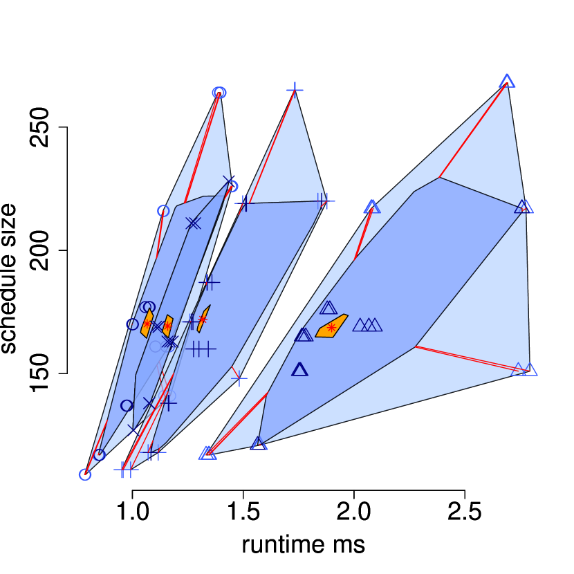
(a) Topologies of size 50.

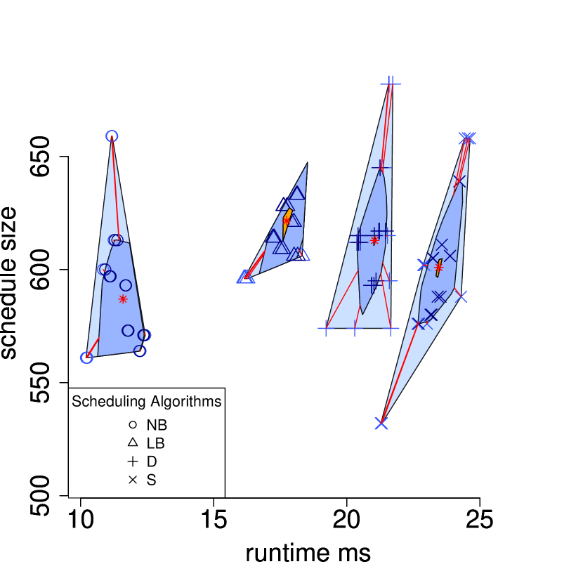
(b) Topologies of size 200.

Figure 2: Normalized bagplots comparing the scheduling algorithm performance for topologies of sizes 50 (left) and 200 (right). Measured runtime is plotted against the produced schedule size. Whereas for the smaller topologies, Dedicated and Shared Scheduling are only slightly slower than Node-Based Scheduling, do the results for the larger topologies indicate that they don’t scale well in the size of the network. The schedule size distributions, read from the y-axis of the plots, overlap largely for both topology sizes, and can therefore not identify a winner in the comparison.

Network Size		50				200
Reliability Algorithm		SchedEx		Incrementer		SchedEx		Incrementer
$\underline{\rho}$	Sched. Alg.	$ms$	$|\mathcal{F}|$	$ms$	$|\mathcal{F}|$	$ms$	$|\mathcal{F}|$	$ms$	$|\mathcal{F}|$
0.9	Node-Based	$\mathbf{5}\pm 3$	$\mathbf{736}\pm 258$	$274\pm 172$	$609\pm 201$	$\mathbf{42}\pm 3$	$\mathbf{1948}\pm 102$	$2021\pm 150$	$1640\pm 59$
	Level-Based	$11\pm 11$	$743\pm 243$	$271\pm 161$	$615\pm 188$	$63\pm 5$	$2053\pm 93$	$2206\pm 125$	$1742\pm 52$
	Dedicated	$7\pm 4$	$751\pm 265$	$284\pm 180$	$609\pm 210$	$79\pm 5$	$2031\pm 101$	$2104\pm 192$	$1668\pm 65$
	Shared	$10\pm 14$	$741\pm 256$	$\mathbf{264}\pm 160$	$\mathbf{606}\pm 192$	$86\pm 3$	$1962\pm 78$	$\mathbf{1963}\pm 111$	$\mathbf{1612}\pm 41$
0.999	Node-Based	$\mathbf{6}\pm 1$	$\mathbf{1083}\pm 366$	$545\pm 318$	$987\pm 307$	$\mathbf{64}\pm 6$	$\mathbf{2794}\pm 124$	$4090\pm 358$	$2558\pm 87$
	Level-Based	$11\pm 3$	$1092\pm 346$	$536\pm 290$	$998\pm 286$	$91\pm 11$	$2944\pm 121$	$4498\pm 292$	$2712\pm 79$
	Dedicated	$10\pm 4$	$1108\pm 375$	$544\pm 324$	$984\pm 318$	$111\pm 9$	$2917\pm 124$	$4153\pm 404$	$2586\pm 99$
	Shared	$8\pm 2$	$1091\pm 363$	$\mathbf{531}\pm 317$	$\mathbf{982}\pm 292$	$123\pm 4$	$2815\pm 82$	$\mathbf{3994}\pm 277$	$\mathbf{2511}\pm 64$
0.99999	Node-Based	$\mathbf{8}\pm 2$	$\mathbf{1428}\pm 468$	$\mathbf{837}\pm 494$	$1366\pm 415$	$\mathbf{86}\pm 6$	$\mathbf{3636}\pm 175$	$6634\pm 667$	$3469\pm 119$
	Level-Based	$13\pm 5$	$1438\pm 438$	$877\pm 508$	$1380\pm 386$	$120\pm 7$	$3838\pm 164$	$7459\pm 490$	$3674\pm 106$
	Dedicated	$12\pm 5$	$1459\pm 480$	$846\pm 506$	$1358\pm 428$	$144\pm 11$	$3804\pm 174$	$6944\pm 756$	$3495\pm 131$
	Shared	$10\pm 2$	$1437\pm 464$	$843\pm 490$	$\mathbf{1356}\pm 394$	$162\pm 7$	$3659\pm 127$	$\mathbf{6462}\pm 543$	$\mathbf{3400}\pm 84$

TABLE II: Execution time in $ms$ and schedule size $|\mathcal{F}|$ for the different scheduling algorithms under three reliability constraints comparing SchedEx and the Incrementer from [8] with reliability stop criterion.

See Table II for a summary of the numeric results for the reliability ensuring simulations with SchedEx and the Incrementer. Listed runtimes for the Incrementer contain both, scheduler runtime and Incrementer runtime. First, SchedEx is significantly faster than the Incrementer. Figure 3(a) shows the distributions for how many times SchedEx is faster than the Incrementer. For $\underline{\rho}=0.9(0.99999)$, SchedEx is in average $31$ ($56$) times, and thereby more than an order of magnitude, faster. Figure 3(b) illustrates the performance improvement over the Incrementer in terms of schedule size. It reveals that, the harsher the constraint, the larger the expected improvement of the schedule over the incremental approach. For $\underline{\rho}=0.9$, SchedEx is expected to create schedules that are in average $21\%$ longer than those from the Incrementer. For $\underline{\rho}=0.99999$, the difference is down to $6\%$.

A signal to noise ratio of 60 dB together with a transmission range of 30 units lead to link qualities not below 67%, which we see as a reasonable assumption for networks that are meant to support mission-critical applications. We would, however, like to mention that choosing a signal to noise ratio of 50 dB leads to SchedEx being 2-3 orders of magnitude faster than the Incrementer, while schedule sizes for the harsh scenarios with $0.99999$ lead to in average $5.3\%$ shorter schedules than the Incrementer. This can partly be explained by the fact that the required schedules become much longer, and that the Incrementer does not scale well in the size of the required schedule frame. SchedEx performs better in the severity of the reliability constraint, and that substantially faster.

For a given scheduling algorithm $SA$ with time complexity $C_{Time}(SA)$, SchedEx increases the time complexity by a summand and a factor according to:

$$SchedEx(SA)\leq O(|\mathcal{T}|)+\tau_{max}\times C_{Time}(SA)$$ (27)

The summand $O(|\mathcal{T}|)$ explains the creation of vector $\overrightarrow{\tau}$, and $\tau_{max}=\max{(\overrightarrow{\tau})}$ explains the worst case increase of a schedule. The smaller the signal-to-noise ratio, the proportionally larger is $\tau_{max}$.

The Incrementer requires two steps. First, the initial schedule creation of $C_{Time}(SA)$, and second, the incremental phase until the stop criterion has been reached, according to the incremental algorithm in [8]. The incremental phase is of complexity $O(|\mathcal{T}|D^{2})$, with $D$ being the size of the eventual frame when reaching the stop criterion, as it in each iteration requires a recalculation of a convex improvement metric over the iteratively increasing schedule frame $F$. Thus, the time complexity for the Incrementer is

$$Incrementer(SA)=C_{Time}(SA)+\Theta(|\mathcal{T}|D^{2}),$$ (28)

with $D$ not known a-priori. The smaller the signal-to-noise ratio, the proportionally larger becomes $D$. Thus, where SchedEx scales linearly in the harshness of the problem does the Incrementer scale quadratic. Further, the average topology requires significantly fewer elementary operations than the worst-case with SchedEx, whereas the Incrementer grows relative to $|\mathcal{T}|D^{2}$. For the Incrementer, the experiments reveal that the scheduling phase with time complexity $C_{Time}(SA)$ stands in our simulations in average for only about $0.003$% of its total runtime, and does therefore not weigh in significantly.

(a)

(b)

Figure 3: The percentual performance improvement of SchedEx over the Incrementer grouped by reliability constraint $\underline{\rho}$. (Left: Time, Right: Schedule Size)

\begin{overpic}[width=346.89731pt]{simpleSAcomparison} \put(22.0,3.0){Basic} \put(45.0,3.0){SchedEx} \put(70.0,3.0){Incrementer} \end{overpic}

Figure 4: The distance to optimum distribution for all four scheduling algorithms given three methods: Basic, SchedEx, and Incrementer.

Figure 5: The difference in required schedule size that can be expected for varying $\underline{\rho}$ over all scheduling algorithms, using SchedEx.

Figure 4 shows the relative distance to the best found solution among the four scheduling algorithms, grouped by the basic scheduling without reliability constraints (Basic), SchedEx, and the Incrementer. The Incrementer favors Dedicated and Shared Scheduling, while SchedEx creates less variance among the scheduling algorithms, suggesting that it is more generic and less sensitive to the specifics of the scheduling algorithm of use. SchedEx produces in average the best schedules with Node-based Scheduling, whereas the Incrementer performs best with Dedicated Scheduling.

Figure 5 illustrates the required schedule size difference for varying $\underline{\rho}$ over all scheduling algorithms. The expected schedule sizes for $\underline{\rho}$ being $0.9,0.999$ and $0.99999$ are $1370$, $1980$, and $2587$, respectively. The schedules can therefore be expected to be ca. 45% longer for a change in harshness from $0.9$ to $0.999$, and ca. 89% longer for a change from $0.9$ to $0.99999$ on the same topology.

With SchedEx, schedules with reliability guarantees can swiftly be calculated. However, for many control applications would the latency implications still not be acceptable. For instance, assuming WirelessHART with slot sizes of 10 ms and $\underline{\rho}=0.99999$, the schedule frame would require about 1430 slots, translating into a delay of 14.3 seconds for one packet from each transmitter to arrive at the destination on topologies of size 50. High node-to-node packet reception rates between the sensors are one way to reduce that number, for instance by installing relays, or using multiple channels.

VII Conclusions

We introduced SchedEx, a generic scheduling algorithm extension which gives reliability guarantees for topologies with guaranteed lower-bounded node-to-node packet reception rates. SchedEx is an order of magnitude faster than the theoretically well developed approach in [8] and the harsher the reliability constraint, the relatively better SchedEx performs. Guaranteeing harsh reliability constraints implies a substantial latency penalty, where the expected difference in schedule size from one nine to five nines is nearly twice the length. As stated in the discussion, guaranteeing reliability bounds has a huge impact on the effected latency bounds. For future work, multi-channel scheduling and multiple sink deployment should be investigated considering the required latency improvements. For instance, WirelessHART uses up to 15 channels to concurrently transmit packets. Other important future scheduling extensions are the consideration of individual latency bounds for different flows, priority handling, and the verification of the simulation results in a testbed. The introduced SchedEx algorithm presents one step towards scalable scheduling, a highly required feature for end-to-end QoS guarantees in WSN.

References

- [1] G. Hancke, V. Gungor, and G. Hancke, “Guest editorial special section on industrial wireless sensor networks,” Industrial Informatics, IEEE Transactions on, vol. 10, no. 1, pp. 762–765, Feb 2014.
- [2] P. Suriyachai, U. Roedig, and A. Scott, “A survey of mac protocols for mission-critical applications in wireless sensor networks,” Communications Surveys Tutorials, IEEE, vol. 14, no. 2, pp. 240–264, 2012.
- [3] K. S. J. Pister and L. Doherty, “Tsmp: Time synchronized mesh protocol,” in In Proceedings of the IASTED International Symposium on Distributed Sensor Networks, 2008.
- [4] G. Bianchi, “Performance analysis of the ieee 802.11 distributed coordination function,” Selected Areas in Communications, IEEE Journal on, vol. 18, no. 3, pp. 535–547, 2000.
- [5] T. Lennvall, S. Svensson, and F. Hekland, “A comparison of wirelesshart and zigbee for industrial applications,” in IEEE International Workshop on Factory Communication Systems, vol. 2008, 2008, pp. 85–88.
- [6] S. Ergen and P. Varaiya, “Tdma scheduling algorithms for wireless sensor networks,” Wireless Networks, vol. 16, pp. 985–997, 2010.
- [7] O. Incel, A. Ghosh, and B. Krishnamachari, “Scheduling algorithms for tree-based data collection in wireless sensor networks,” in Theoretical Aspects of Distributed Computing in Sensor Networks. Springer Berlin Heidelberg, 2011, pp. 407–445.
- [8] M. Yan, K.-Y. Lam, S. Han, E. Chan, Q. Chen, P. Fan, D. Chen, and M. Nixon, “Hypergraph-based data link layer scheduling for reliable packet delivery in wireless sensing and control networks with end-to-end delay constraints,” Information Sciences, vol. 278, pp. 34–55, 2014.
- [9] P. Djukic and S. Valaee, “Delay aware link scheduling for multi-hop tdma wireless networks,” IEEE/ACM Trans. Netw., vol. 17, no. 3, pp. 870–883, Jun. 2009.
- [10] W. Shen, T. Zhang, M. Gidlund, and F. Dobslaw, “Sas-tdma: a source aware scheduling algorithm for real-time communication in industrial wireless sensor networks,” Wireless networks, vol. 19, no. 6, pp. 1155–1170, 2013.
- [11] “Wirelesshart technology,” HART communication foundation, Tech. Rep., Dec 2009.
- [12] “Wireless systems for industrial automation: Process control and related applications,” International Society of Automation (ISA), Standard ISA-100.11a, 2009.
- [13] “IEC 62601 ed1.0, industrial communication network - fieldbus specifications - WIA-PA communication network and communication profile,” 2011.
- [14] “IEEE standard for local and metropolitan area networks - part 15.4: Low-rate wireless personal area networks (lr-wpans) - amendment 1: Mac sublayer, ieee std. 802.15.4e,” IEEE, 2012.
- [15] E. Felemban, C.-G. Lee, and E. Ekici, “Mmspeed: multipath multi-speed protocol for qos guarantee of reliability and. timeliness in wireless sensor networks,” Mobile Computing, IEEE Transactions on, vol. 5, no. 6, pp. 738–754, 2006.
- [16] S.-e. Yoo, P. K. Chong, D. Kim, Y. Doh, M.-L. Pham, E. Choi, and J. Huh, “Guaranteeing real-time services for industrial wireless sensor networks with ieee 802.15. 4,” Industrial Electronics, IEEE Transactions on, vol. 57, no. 11, pp. 3868–3876, 2010.
- [17] E. Toscano and L. Lo Bello, “Multichannel superframe scheduling for ieee 802.15. 4 industrial wireless sensor networks,” Industrial Informatics, IEEE Transactions on, vol. 8, no. 2, pp. 337–350, 2012.
- [18] W. Shen, T. Zhang, F. Barac, and M. Gidlund, “Prioritymac: A priority-enhanced mac protocol for critical traffic in industrial wireless sensor and actuator networks,” Industrial Informatics, IEEE Transactions on, vol. 10, no. 1, 2014.
- [19] N. Marchenko, T. Andre, G. Brandner, W. Masood, and C. Bettstetter, “An experimental study of selective cooperative relaying in industrial wireless sensor networks,” Industrial Informatics, IEEE Transactions on, vol. 10, no. 3, 2014.
- [20] P. Suriyachai, J. Brown, and U. Roedig, “Time-critical data delivery in wireless sensor networks,” in Proceedings of the 6th IEEE international conference on Distributed Computing in Sensor Systems, 2010, pp. 216–229.
- [21] S. Munir, S. Lin, E. Hoque, S. M. S. Nirjon, J. A. Stankovic, and K. Whitehouse, “Addressing burstiness for reliable communication and latency bound generation in wireless sensor networks,” in Proceedings of the 9th ACM/IEEE International Conference on Information Processing in Sensor Networks, ser. IPSN ’10, 2010, pp. 303–314.
- [22] F. Barac, M. Gidlund, and T. Zhang, “Scrutinizing bit-and symbol-errors of ieee 802.15. 4 communication in industrial environments,” Instrumentation and Measurements, IEEE Transactions on, vol. 63, no. 7, 2014.
- [23] E. Felemban, C.-G. Lee, and E. Ekici, “Mmspeed: multipath multi-speed protocol for qos guarantee of reliability and. timeliness in wireless sensor networks,” Mobile Computing, IEEE Transactions on, vol. 5, no. 6, pp. 738–754, 2006.
- [24] R. Fonseca, O. Gnawali, K. Jamieson, and P. Levis, “Four-bit wireless link estimation,” in Proceedings of the Sixth Workshop on Hot Topics in Networks (HotNets VI), vol. 2007, 2007.
- [25] D. Stanislowski, X. Vilajosana, Q. Wang, T. Watteyne, and K. S. Pister, “Adaptive synchronization in ieee802. 15.4 e networks,” Industrial Informatics, IEEE Transactions on, vol. 10, no. 1, pp. 795–802, 2014.
- [26] D. S. De Couto, D. Aguayo, J. Bicket, and R. Morris, “A high-throughput path metric for multi-hop wireless routing,” Wireless Networks, vol. 11, no. 4, pp. 419–434, 2005.
- [27] F. Barac, M. Gidlund, and T. Zhang, “Ubiquitous, yet deceptive: Hardware-based channel metrics on interfered wsn links,” Vehicular Technology, IEEE Transactions on, 2014.
- [28] Q. Liu, S. Zhou, and G. B. Giannakis, “Cross-layer combining of adaptive modulation and coding with truncated arq over wireless links,” Wireless Communications, IEEE Transactions on, vol. 3, no. 5, pp. 1746–1755, 2004.
- [29] V. Ç. Güngör and G. P. Hancke, Industrial Wireless Sensor Networks: Applications, Protocols, and Standards. CRC Press, 2013.