Geometric pumping induced by shear flow in dilute liquid crystalline polymer solutions

Abstract

We investigate nonlinear rheology of dilute liquid crystalline polymer solutions under time dependent two-directional shear flow. We analyze the Smoluchowski equation, which describes the dynamics of the orientation of a liquid crystalline polymer, by employing technique of the full counting statistics. In the adiabatic limit, we derive the expression for time integrated currents generated by a Berry-like curvature. Using this expression, it is shown that the expectation values of the time-integrated angular velocity of a liquid crystalline polymer and the time-integrated stress tensor are generally not zero even if the time average of the shear rate is zero. The validity of the theoretical calculations is confirmed by direct numerical simulations of the Smoluchowski equation. Nonadiabatic effects are also investigated by means of simulations and it is found that the time-integrated stress tensor depends on the speed of the modulation of the shear rate if we adopt the isotropic distribution as an initial state.

I Introduction

Recently, nonlinear transport phenomena in stochastic processes under an adiabatic modulation of the externally controlled parameters have attracted much attention. It is found that a current is generated under modulation even if there is no mean bias because of the existence of a geometrical phase which are analogous to Berry’s phase Berry ; Samuel Bhandari ; Thouless ; Sinisyn ; Sinitsyn2 ; Ohkubo ; Chernyak . We call such phenomena geometric pumping in this paper. In the context of steady state thermodynamics, Sagawa and Hayakawa obtained the geometric expression of the excess entropy production for a Markov Jump process Sagawa-Hayakawa . We also note that similar phenomena in quantum dot systems were investigated by means of quantum master equations Ren Hanggi Li ; Yuge . The nonadiabatic effects in quantum pumping for a spin-boson system were also investigated recently Watanabe hayakawa . So far, however, most of these studies were limited only to simple jump processes and quantum dot systems. It may be of great interest to verify whether similar effects exist even in macroscopic systems using the framework of the geometrical pumping process.

We focus on dilute liquid crystalline polymer solutions in this paper as one of the simplest macroscopic systems where we can apply idea of the geometrical pumping. Note that liquid crystalline polymers are characterized by their high rigidity. Thus, for instance, a helix structure of some polypeptide and tobacco mosaic viruses can be regarded as hard rods Doi-Edwards ; de Gennes Prost . It is known that the macroscopic rheological behavior of liquid crystalline polymer solutions as well as the dynamics of the orientation of a liquid crystalline polymer can be described in terms of the Smoluchowski equation Doi-Edwards . We analyze the Smoluchowski equation by applying the framework of Ref. Sagawa-Hayakawa .

The behavior of liquid crystalline polymers under shear flows has been studied extensively Nemoto ; Ookubo . The polymer motion is influenced by the shear flow, while the conformation dynamics of polymers influence the rheological properties of the polymer solution Doi-Edwards . Harasim et al. recently observed the dynamics of f-actins under a steady shear flow and found that polymers undergo tumbling motion but the periods of tumbling motion are stochastically fluctuating Harasim . Recently, van Leeuwen and Blöte carried out numerical simulations of dynamics of a rod-like particle under a shear flow in the large Weissenberg number regime and obtained asymptotic behavior of the average of the angular velocity van Leeuwen Blote . We note that there are several studies on nonlinear rheology of dilute liquid crystalline polymers, they mostly focus on steady states and the effects of shear modulation have not been investigated systematically Hinch Leal ; Hinch Leal2 ; Stewart Sorensen .

In this paper, we consider situations where there is time-dependent two-directional shear flow. We investigate the averaged angular velocity of rods and the macroscopic stress tensor under adiabatic modulation of the two shear rates. It is shown that one component of the time-integrated angular velocity of the rod and one component of the time-integrated stress tensor are generally not zero even if the time average of the shear rate is zero. The former result suggests that the rod can work as a microscopic or nano machine that converts the angular velocity of the external shear flow to the rotation of the rod under thermally fluctuating environment. The latter result suggests that geometric pumping effect of a single rod is related to a novel rheological response of macroscopic dilute liquid crystalline solutions.

The organization of this paper is as follows. In Section II, we briefly review the Smoluchowski equation, which is employed to describe the dynamics of orientation of a hard rod under external flow. In Section III, we formulate the full counting statistics to derive the decomposition of the time integrated current into the housekeeping and excess parts under adiabatic modulation of externally controlled parameters. In Section IV, we numerically calculate the excess angular velocity and the excess stress tensor under two adiabatic shear rate protocols. We confirm that the theoretically predicted values calculated from the expression obtained in Section III agree well with those obtained by direct numerical simulations of the Smoluchowski equation in adiabatic condition.

II Model

In this section, we briefly explain the model we use, and explain the general framework of Smoluchowski equation. We consider a dilute solution of liquid crystalline polymers under a time-dependent uniform shear rate tensor:

$$v_{\alpha}\left(\vec{x},t\right)=\kappa_{\alpha\beta}\left(t\right)x_{\beta},$$ (1)

where $\kappa_{\alpha\beta}\left(t\right)$ is the velocity gradient tensor. Here, we adopt Einstein summation convention when an index variable appears twice throughout this paper. In this paper, we consider the two-directional shear rate tensor:

$$\kappa_{\alpha\beta}\left(t\right)=\left(f_{1}\left(t\right)\delta_{\alpha x}+f_{2}\left(t\right)\delta_{\alpha y}\right)\delta_{\beta z}.$$ (2)

We assume that the shear flow is periodic in time: $f_{i}\left(t_{f}\right)=f_{i}\left(0\right)$. We assume that the polymers are rigid to regard them as straight hard rods with an identical length. We denote the orientation of the long-axis of a rod as $\vec{u}$ which satisfies $\left|\vec{u}\right|=1$. We ignore the interactions between polymers. We also assume that the distribution function $\Psi\left(\vec{u},t\right)$ is spatially uniform.

Each rod undergoes rotational Brownian motion as well as translational Brownian motion due to thermal fluctuations. In overdamped cases, the Langevin equation for the orientation of each polymer is given by Doi-Edwards

$$\frac{d\vec{u}}{dt}=-\vec{\nabla}U\left(\vec{u}\right)+\overleftrightarrow{\kappa}\left(t\right)\cdot\vec{u}-\vec{u}\left(\vec{u}\cdot\overleftrightarrow{\kappa}\left(t\right)\cdot\vec{u}\right)+\vec{\xi},$$ (3)

where we have introduced the potential $U\left(\vec{u}\right)$ which represents a softening constraint of $\left|\vec{u}\right|=1$ and a zero-mean Gaussian white noise $\vec{\xi}\left(t\right)$ which satisfies

$$\left\langle\vec{\xi}\left(t\right)\vec{\xi}\left(t^{\prime}\right)\right\rangle=2D_{r}\delta\left(t-t^{\prime}\right)\overleftrightarrow{1},$$ (4)

where $D_{r}$ is the rotational diffusion constant. We note that $\vec{u}$ is a dimensionless vector, and therefore, $D_{r}$ has the dimension of the inverse of time. The terms $\overleftrightarrow{\kappa}\cdot\vec{u}-\vec{u}\left(\vec{u}\cdot\overleftrightarrow{\kappa}\cdot\vec{u}\right)$ represent the rotation of rods under the shear rate $\kappa_{\alpha\beta}\left(t\right)$. It is known that Eq. (3) is equivalent to the following Smoluchowski equation Doi-Edwards .

$$\frac{\partial\Psi}{\partial t}=D_{r}\mathcal{R}\cdot\mathcal{R}\Psi-\mathcal{R}\cdot\left(\vec{u}\times\overleftrightarrow{\kappa}\left(t\right)\cdot\vec{u}\Psi\right)$$ (5)

Here we have introduced the rotational operator $\mathcal{R}$ as

$$\mathcal{R}=\vec{u}\times\frac{\partial}{\partial\vec{u}}.$$ (6)

The first term on the right hand side (RHS) of Eq. (5) describes the rotational diffusion of rod orientation, and the second term represents the deterministic rotation of rods under the external flow.

For dilute liquid crystalline polymers, the macroscopic stress tensor $\sigma_{\alpha\beta}$ can be decomposed into two partsDoi-Edwards ; Hinch Leal ; Hinch Leal2 :

$$\sigma_{\alpha\beta}=\sigma_{\alpha\beta}^{\left(e\right)}+\sigma_{\alpha\beta}^{\left(v\right)},$$ (7)

where the elastic contribution $\sigma_{\alpha\beta}^{\left(e\right)}$ and the viscous contribution $\sigma_{\alpha\beta}^{\left(v\right)}$ are given by

$$\sigma_{\alpha\beta}^{\left(e\right)}=k_{B}T\nu\left\langle 3\left(u_{\alpha}u_{\beta}-\frac{1}{3}\delta_{\alpha\beta}\right)\right\rangle,$$ (8)

$$\sigma_{\alpha\beta}^{\left(v\right)}=\frac{k_{B}T\nu}{2D_{r}}\left\langle u_{\alpha}u_{\beta}u_{\mu}u_{\nu}\right\rangle\kappa_{\mu\nu}\left(t\right),$$ (9)

where $\nu$ is the number of polymers in unit volume. The elastic contribution $\sigma_{\alpha\beta}^{\left(e\right)}$ represents the free energy increment due to the orientation alignment induced by the external flow and the viscous contribution $\sigma_{\alpha\beta}^{\left(v\right)}$ comes from the dissipation of the free energy due to the friction between the rod and the surrounding fluid. We note that the viscous contribution depends on how we treat the hydrodynamic interaction between the monomers in a liquid crystalline polymer. The coefficient $\frac{k_{B}T\nu}{2D_{r}}$ is evaluated using the so-called shish-kebab model Doi-Edwards ; Hinch Leal ; Hinch Leal2 .

Next, let us introduce the integrated angular velocity and stress tensor $J_{1}$ and $J_{2}$:

$$J_{1}=\int_{0}^{t_{f}}dt\left[\vec{u}\times\overleftrightarrow{\kappa}\left(t\right)\cdot\vec{u}\right]_{x}$$ (10)

$$J_{2}=\int_{0}^{t_{f}}dt\sigma_{yz}=k_{B}T\nu\int_{0}^{t_{f}}dt\left[3u_{y}u_{z}+\frac{1}{2D_{r}}u_{y}u_{z}u_{\mu}u_{\nu}\kappa_{\mu\nu}\left(t\right)\right]$$ (11)

In this paper we consider how the statistical average of these integrated currents $J_{1}$ and $J_{2}$ depend on the time dependent shear rate $\kappa_{\alpha\beta}\left(t\right)$.

III Formulation

In this section, we consider the average value of the time integrated quantity

$$J=\int_{0}^{t_{f}}dt^{\prime}H\left(\vec{u},\left\{\kappa_{j}\left(t^{\prime}\right)\right\}\right)$$ (12)

and derive the expression of the excess part of $J$ under time dependent shear rate $\overleftrightarrow{\kappa}\left(t\right)$. Throughout this paper $H\left(\vec{u},\left\{\kappa_{j}\left(t^{\prime}\right)\right\}\right)$ represents an arbitrary function. To prove our results, we use the technique of the full counting statistics Sinitsyn review ; Okubo review , which makes use of the cumulant generating function

$$S\left(i\chi\right)=\ln\int dJe^{i\chi J}P\left(J\right),$$ (13)

following Ref. Sagawa-Hayakawa by Sagawa and Hayakawa. They applied the adiabatic approximation to the cumulant generating function and obtained a geometric expression of the excess currents. First, we develop our formulation for a Brownian particle under a potential. Next, we will impose the constraint $\left|\vec{u}\right|=1$ as by adding a steep potential as in Eq. (3) and we derive the expression of the excess part of a time-integrated quantity for a rod.

III.1 A Brownian particle under a potential

We consider a Brownian particle in three dimensional space under external force $\vec{f}\left(\vec{x},\left\{\kappa_{j}\left(t\right)\right\}\right)$ depending on the control parameters $\left\{\kappa_{j}\left(t\right)\right\}$. Here, we assume that the motion of the Brownian particle is described by the Langevin equation:

$$\dot{\vec{x}} = \vec{f}\left(\vec{x},\left\{\kappa_{j}\left(t\right)\right\}\right)+\vec{\xi}\left(t\right),$$ (14)

where $\vec{\xi}\left(t\right)$ is a zero-mean Gaussian white noise satisfying

$$\left\langle\vec{\xi}\left(t\right)\vec{\xi}\left(t^{\prime}\right)\right\rangle=2D\delta\left(t-t^{\prime}\right)\overleftrightarrow{1},$$ (15)

where $D$ is the diffusion constant. We introduce the initial probability distribution $P_{0}\left(\vec{x}_{0}\right)$ at the particle position $\vec{x}_{0}$. Here, we only consider a protocol satisfying $\left\{\kappa_{j}\left(t_{f}\right)\right\}=\left\{\kappa_{j}\left(0\right)\right\}$. In order to write down the path-integral expression of path probability, we first discretize time $t$ as

$$t_{n}=n\epsilon$$ (16)

for $n=0,1,\cdots,N$ and we take $\epsilon$ as $N\epsilon=t_{f}$. We will take the continuous-time limit $\epsilon\rightarrow 0$ in deriving the continuous-time expression. By employing It$\bar{\mathrm{o}}$ calculus, we discretize the Langevin equation given by Eq. (14) as

$$\vec{x}_{n+1} = \vec{x}_{n}+\vec{f}\left(\vec{x}_{n},\left\{\kappa_{j}\left(\epsilon n\right)\right\}\right)\epsilon+\vec{\xi}_{n}\epsilon$$ (17)

$$= \vec{x}_{0}+\epsilon\sum_{i=0}^{n}\left(\vec{f}\left(\vec{x}_{i},\left\{\kappa_{j}\left(\epsilon i\right)\right\}\right)+\vec{\xi}_{i}\right).$$

Here we now convert the Gaussian noise in Eq. (14) by $\vec{\xi}_{i}$ $(i=0,1,\cdots,N-1)$ which satisfies

$$<\vec{\xi}_{i}>=0,\quad\left\langle\vec{\xi}_{i}\vec{\xi}_{j}\right\rangle=\frac{2D}{\epsilon}\delta_{ij}\overleftrightarrow{1}.$$ (18)

The distribution function for $\vec{\xi}_{i}$ is given by

$$P\left(\vec{\xi}_{0},\cdots,\vec{\xi}_{N-1}\right)=\left(\frac{\epsilon}{4\pi D}\right)^{3N/2}\exp\left[-\frac{\epsilon}{4D}\sum_{i=0}^{N-1}\vec{\xi}_{i}^{2}\right]$$ (19)

Then we convert the variable $\vec{\xi}_{i}$ to $\vec{x}_{i}$ in the above distribution function $P\left(\vec{\xi}_{0},\cdots,\vec{\xi}_{N-1}\right)$ by using Eq. (17). The Jacobi matrix $\left(\frac{\partial x_{k}}{\partial\xi_{l}}\right)$ is an upper triangular matrix if we take the row elements as $\left\{x_{N,1},x_{N,2},x_{N,3},x_{N-1,1},x_{N-1,2},x_{N-1,3},\cdots,x_{1,1},x_{1,2},x_{1,3}\right\}$ and the line elements as $\left\{\xi_{N-1,1},\xi_{N-1,2},\xi_{N-1,3},\xi_{N-2,1},\xi_{N-2,2},\xi_{N-2,3},\cdots,\xi_{0,1},\xi_{0,2},\xi_{0,3}\right\}$. Then, the Jacobian of the transformation $\vec{\xi}_{i}$ to $\vec{x}_{i}$ is given by

$$\left|\frac{\partial\left(\vec{x}_{1},\cdots,\vec{x}_{N}\right)}{\partial\left(\vec{\xi}_{0},\cdots,\vec{\xi}_{N-1}\right)}\right|=\epsilon^{3N}.$$ (20)

Thus we obtain the probability distribution function for a discretized path $\vec{x}_{0},\vec{x}_{1},\cdots,\vec{x}_{N}$ :

$$P\left(\vec{x}_{0},\vec{x}_{1},\cdots,\vec{x}_{N}\right)=\frac{1}{\epsilon^{3N}}\left(\frac{\epsilon}{4\pi D}\right)^{3N/2}\exp\left[-\frac{\epsilon}{4D}\sum_{i=0}^{N-1}\left(\frac{\vec{x}_{i+1}-\vec{x}_{i}}{\epsilon}-\vec{f}\left(\vec{x}_{i},\left\{\kappa_{j}\left(\epsilon i\right)\right\}\right)\right)^{2}\right].$$ (21)

Then the cumulant generating function for this discretized process is expressed as

$$S\left(i\chi\right) =\ln\int dJe^{i\chi J}P\left(J\right)$$

$$=\ln\int d^{3}xF_{N}\left(i\chi,\vec{x}\right),$$ (22)

where $\chi\in\mathbb{R}$ is the counting field. Here we have introduced the probability distribution function $P\left(J\right)$ and a function $F_{m}\left(i\chi,\vec{x}\right)$ $(m=1,2,\cdots,N)$ as

$$P\left(J\right)=\frac{1}{\epsilon^{3N}}\left(\frac{\epsilon}{4\pi D}\right)^{3N/2}\int\prod_{i=0}^{N}d^{3}x_{i}P\left(\vec{x}_{0},\vec{x}_{1},\cdots,\vec{x}_{N}\right)\delta\left(J-\epsilon\sum_{i=0}^{N-1}H\left(\vec{x}_{i},\left\{\kappa_{j}\left(\epsilon i\right)\right\}\right)\right)P_{0}\left(\vec{x}_{0}\right),$$ (23)

$$F_{m}\left(i\chi,\vec{x}\right) = \frac{1}{\epsilon^{3m}}\left(\frac{\epsilon}{4\pi D}\right)^{3m/2}\int\prod_{i=0}^{m-1}d^{3}x_{i}\exp\left[i\chi\epsilon\sum_{i=0}^{m-1}H\left(\vec{x}_{i},\left\{\kappa_{j}\left(\epsilon i\right)\right\}\right)\right]$$ (24)

$$\times\exp\left[-\frac{\epsilon}{4D}\sum_{i=0}^{m-1}\left(\frac{\vec{x}_{i+1}-\vec{x}_{i}}{\epsilon}-\vec{f}\left(\vec{x}_{i},\left\{\kappa_{j}\left(\epsilon i\right)\right\}\right)\right)^{2}\right]P_{0}\left(\vec{x}_{0}\right),$$

where $\vec{x}_{m}$ is fixed as $\vec{x}_{m}=\vec{x}$ in Eq. (24). We can interpret $F_{m}\left(i\chi,\vec{x}\right)$ as the path-integration of the path probability multiplied by the phase factor $\exp\left[i\chi\int_{0}^{m\epsilon}H\left(\vec{x}\left(t\right),\left\{\kappa_{j}\left(t^{\prime}\right)\right\}\right)dt\right]\cong\exp\left[i\chi\epsilon\sum_{i=0}^{m-1}H\left(\vec{x}_{i},\left\{\kappa_{j}\left(t^{\prime}\right)\right\}\right)\right]$ with respect to the all paths which satisfy $\vec{x}\left(m\epsilon\right)=\vec{x}$. In the continuous time limit $\epsilon\rightarrow 0$, we denote the continuous time limit of $F_{m}\left(i\chi,\vec{x}\right)$ as

$$F\left(i\chi,\vec{x},t\right)\cong F_{m}\left(i\chi,\vec{x}\right),$$ (25)

where $t\cong m\epsilon$. From the definition of $F\left(i\chi,\vec{x},t\right)$ in Eqs. (24) and (25), we express the average value of $\int_{0}^{t}dt^{\prime}H\left(\vec{x},\left\{\kappa_{j}\left(t^{\prime}\right)\right\}\right)$ as

$$\left\langle\int_{0}^{t}dt^{\prime}H\left(\vec{x},\left\{\kappa_{j}\left(t^{\prime}\right)\right\}\right)\right\rangle$$ (26)

$$= \frac{1}{i}\left(\frac{\partial S\left(i\chi\right)}{\partial\chi}\right)_{\chi=0}$$

$$= \int d^{3}x\frac{1}{i}\left(\frac{\partial F\left(i\chi,\vec{x},t\right)}{\partial\chi}\right)_{\chi=0}\left(\int d^{3}x^{\prime}F\left(0,\vec{x^{\prime}},t\right)\right)^{-1}$$

$$= \int d^{3}x\frac{1}{i}\left(\frac{\partial F\left(i\chi,\vec{x},t\right)}{\partial\chi}\right)_{\chi=0},$$

where $\left\langle\cdots\right\rangle$ represents the statistical average. To obtain the last expression we have used the following relation.

$$\int d^{3}x^{\prime}F\left(0,\vec{x^{\prime}},t\right)=1$$ (27)

Next, let us evaluate $F\left(i\chi,\vec{x},t\right)$. As in Appendix A,

$$\frac{dF}{dt}\left(i\chi,\vec{x},t\right) = -\frac{\partial}{\partial x_{k}}\left[\left(\vec{f}\left(\vec{x},\left\{\kappa_{j}\left(t\right)\right\}\right)\right)_{k}F\left(i\chi,\vec{x},t\right)\right]+D\nabla^{2}F\left(i\chi,\vec{x},t\right)$$ (28)

$$+i\chi\left(H\left(\vec{x},\left\{\kappa_{j}\left(t\right)\right\}\right)\right)F\left(i\chi,\vec{x},t\right)$$

$$= \mathcal{K}\left(\chi,\left\{\kappa_{j}\left(t\right)\right\}\right)F\left(i\chi,\vec{x},t\right),$$

where the operator $\mathcal{K}\left(\chi,\left\{\kappa_{j}\left(t\right)\right\}\right)$ in the last expression of Eq. (28) acting on an arbitrary function $a(\vec{x})$ is given by

$$\mathcal{K}\left(\chi,\left\{\kappa_{j}\left(t\right)\right\}\right)a\left(\vec{x}\right) = -\frac{\partial}{\partial x_{k}}\left[\left(\vec{f}\left(\vec{x},\left\{\kappa_{j}\left(t\right)\right\}\right)\right)_{k}a\left(\vec{x}\right)\right]+D\nabla^{2}a\left(\vec{x}\right)$$ (29)

$$+i\chi\left(H\left(\vec{x},\left\{\kappa_{j}\left(t\right)\right\}\right)\right)a\left(\vec{x}\right).$$

We denote the eigenfunction of $\mathcal{K}\left(\chi,\left\{\kappa_{j}\left(t\right)\right\}\right)$ for the $n$-th largest real part by $f_{\chi}^{n}\left(\left\{\kappa_{j}\left(t^{\prime}\right)\right\},\vec{x}\right)$ and its eigenvalue by $\lambda_{\chi}^{n}\left(\left\{\kappa_{j}\left(t^{\prime}\right)\right\}\right)$. When we set $\chi=0$, Eq. (28) reduces to the Fokker-Planck equation for the probability distribution function $P\left(\vec{x},t\right)=F\left(0,\vec{x},t\right)$. We assume that the Fokker-Planck operator $\mathcal{K}\left(0,\left\{\kappa_{j}\left(t\right)\right\}\right)$ is diagonalizable and $\lambda_{\chi=0}^{0}\left(\left\{\kappa_{j}\left(t^{\prime}\right)\right\}\right)=0$ is not degenerated. When $\left|\chi\right|$ is sufficiently small, $\mathcal{K}\left(\chi,\left\{\kappa_{j}\left(t\right)\right\}\right)$ can be also diagonalized and $\lambda_{\chi}^{0}\left(\left\{\kappa_{j}\left(t^{\prime}\right)\right\}\right)$ is not degenerated. In order to solve the above equation, we expand $F\left(i\chi,\vec{x},t\right)$ in terms of the eigenfunctions as

$$F\left(i\chi,\vec{x},t\right)=\sum_{n}c_{n}\left(t\right)\exp\left[\int_{0}^{t}dt^{\prime}\lambda_{\chi}^{n}\left(\left\{\kappa_{j}\left(t^{\prime}\right)\right\}\right)\right]f_{\chi}^{n}\left(\left\{\kappa_{j}\left(t^{\prime}\right)\right\},\vec{x}\right).$$ (30)

Using Eq. (28), we readily obtain

$$\dot{c}_{0}\left(t\right) = -\int d^{3}x\tilde{f_{\chi}^{0}}\left(\left\{\kappa_{j}\left(t^{\prime}\right)\right\},\vec{x}\right)\sum_{n}c_{n}\left(t\right)\exp\left[\int_{0}^{t}dt^{\prime}\left[\lambda_{\chi}^{n}\left(\left\{\kappa_{j}\left(t^{\prime}\right)\right\}\right)-\lambda_{\chi}^{0}\left(\left\{\kappa_{j}\left(t^{\prime}\right)\right\}\right)\right]\right]$$ (31)

$$\times\left(\frac{\partial}{\partial\kappa_{k}}f_{\chi}^{n}\left(\left\{\kappa_{j}\left(t^{\prime}\right)\right\},\vec{x}\right)\right)\dot{\kappa}_{k}\left(t^{\prime}\right),$$

where we have introduced the left eigenvector $\tilde{f_{\chi}^{m}}\left(\left\{\kappa_{j}\left(t^{\prime}\right)\right\},\vec{x}\right)$ satisfying

$$\int d^{3}x\tilde{f_{\chi}^{m}}\left(\left\{\kappa_{j}\left(t^{\prime}\right)\right\},\vec{x}\right)f_{\chi}^{n}\left(\left\{\kappa_{j}\left(t^{\prime}\right)\right\},\vec{x}\right)=\delta_{n,m},$$ (32)

$$\mathcal{K}^{\dagger}\left(\chi,\left\{\kappa_{j}\left(t\right)\right\}\right)\tilde{f_{\chi}^{n}}\left(\left\{\kappa_{j}\left(t^{\prime}\right)\right\},\vec{x}\right) = \lambda_{\chi}^{n}\tilde{f_{\chi}^{n}}\left(\left\{\kappa_{j}\left(t^{\prime}\right)\right\},\vec{x}\right),$$ (33)

$$\left(\tilde{f_{\chi}^{0}}\left(\left\{\kappa_{j}\left(t^{\prime}\right)\right\},\vec{x}\right)\right)_{\chi=0}=1.$$ (34)

Here the operator $\mathcal{K}^{\dagger}\left(\chi,\left\{\kappa_{j}\left(t\right)\right\}\right)$ is the conjugate to $\mathcal{K}\left(\chi,\left\{\kappa_{j}\left(t\right)\right\}\right)$ acting on an arbitrary function $a\left(\vec{x}\right)$ as

$$\mathcal{K}^{\dagger}\left(\chi,\left\{\kappa_{j}\left(t\right)\right\}\right)a\left(\vec{x}\right)= \left(\vec{f}\left(\vec{x},\left\{\kappa_{j}\left(t\right)\right\}\right)\right)_{k}\frac{\partial}{\partial x_{k}}a\left(\vec{x}\right)+D\nabla^{2}a\left(\vec{x}\right)$$

$$+i\chi\left(H\left(\vec{x},\left\{\kappa_{j}\left(t\right)\right\}\right)\right)a\left(\vec{x}\right).$$ (35)

If we modulate the control parameter much slower than a typical relaxation rate of the system, the contributions from $c_{n}\left(t\right)\left(n\neq 0\right)$ in Eq. (30) are negligible and we obtain

$$F\left(i\chi,\vec{x},t\right) \cong c_{0}\left(i\chi\right)f_{\chi}^{0}\left(\left\{\kappa_{j}\left(t\right)\right\},\vec{x}\right)\exp\left[\int_{0}^{t}dt^{\prime}\lambda_{\chi}^{0}\left(\left\{\kappa_{j}\left(t^{\prime}\right)\right\}\right)\right]$$ (36)

$$\times\exp\left(-\int_{0}^{t}dt^{\prime}\int d^{3}x\tilde{f_{\chi}^{0}}\left(\left\{\kappa_{j}\left(t^{\prime}\right)\right\},\vec{x}\right)\right.$$

$$\left.\times\left(\frac{\partial}{\partial\kappa_{k}}f_{\chi}^{0}\left(\left\{\kappa_{j}\left(t^{\prime}\right)\right\},\vec{x}\right)\right)\dot{\kappa}_{k}\left(t^{\prime}\right)\right),$$

where we have assumed that the real part of $\lambda_{\chi}^{n}\left(\left\{\kappa_{j}\left(t^{\prime}\right)\right\}\right)-\lambda_{\chi}^{0}\left(\left\{\kappa_{j}\left(t^{\prime}\right)\right\}\right)$ is negative for $n\neq 0$. We also assume

$$c_{0}\left(i\chi\right)=\int d^{3}x\tilde{f_{\chi}^{0}}\left(\left\{\kappa_{j}\left(0\right)\right\},\vec{x}\right)\left(f_{\chi}^{0}\left(\left\{\kappa_{j}\left(0\right)\right\},\vec{x}\right)\right)_{\chi=0},$$ (37)

i.e. the initial state is the stationary state $\left(f_{\chi}^{0}\left(\left\{\kappa_{j}\left(0\right)\right\},\vec{x}\right)\right)_{\chi=0}$ for the initial control parameter $\left\{\kappa_{j}\left(0\right)\right\}$. Using Eqs. (26), (32), (34), (36) and (37), we can evaluate the average $\left\langle\int_{0}^{t_{f}}dt^{\prime}H\left(\vec{x},\left\{\kappa_{j}\left(t^{\prime}\right)\right\}\right)\right\rangle$ as

$$\left\langle\int_{0}^{t_{f}}dt^{\prime}H\left(\vec{x},\left\{\kappa_{j}\left(t^{\prime}\right)\right\}\right)\right\rangle$$

$$= \int d^{3}x\frac{1}{i}\left(\frac{\partial F\left(i\chi,\vec{x},t_{f}\right)}{\partial\chi}\right)_{\chi=0}$$

$$= -\frac{1}{i}\int_{0}^{t_{f}}dt^{\prime}\int d^{3}x\left(\frac{\partial\tilde{f_{\chi}^{0}}}{\partial\chi}\left(\left\{\kappa_{j}\left(t^{\prime}\right)\right\},\vec{x}\right)\sum_{k}\left(\frac{\partial}{\partial\kappa_{k}}f_{\chi}^{0}\left(\left\{\kappa_{j}\left(t^{\prime}\right)\right\},\vec{x}\right)\dot{\kappa}_{k}\left(t^{\prime}\right)\right)\right)_{\chi=0}$$

$$+\int_{0}^{t_{f}}dt^{\prime}H_{hk}\left(\left\{\kappa_{j}\left(t^{\prime}\right)\right\}\right)$$

$$+\int d^{3}x\frac{1}{i}\left(\frac{\partial f_{\chi}^{0}}{\partial\chi}\left(\left\{\kappa_{j}\left(t_{f}\right)\right\},\vec{x}\right)\right)_{\chi=0}$$

$$-\int d^{3}x\frac{1}{i}\left(f_{\chi}^{0}\left(\left\{\kappa_{j}\left(t_{f}\right)\right\},\vec{x}\right)\int d^{3}x^{\prime}\left(\frac{\partial f_{\chi}^{0}}{\partial\chi}\left(\left\{\kappa_{j}\left(t_{f}\right)\right\},\vec{x^{\prime}}\right)-\frac{\partial f_{\chi}^{0}}{\partial\chi}\left(\left\{\kappa_{j}\left(0\right)\right\},\vec{x^{\prime}}\right)\right)\right)_{\chi=0}$$

$$+\left(\frac{1}{i}\frac{\partial c_{0}}{\partial\chi}\left(i\chi\right)\right)_{\chi=0},$$ (38)

where we have defined the housekeeping part of the current as $H_{hk}\left(\left\{\kappa_{j}\left(t^{\prime}\right)\right\}\right)\equiv\frac{1}{i}\left(\frac{\partial\lambda_{\chi}^{0}}{\partial\chi}\left(\left\{\kappa_{j}\left(t^{\prime}\right)\right\}\right)\right)_{\chi=0}$. The housekeeping part represents the average current $\left\langle H\left(\vec{x},\left\{\kappa_{j}\left(t^{\prime}\right)\right\}\right)\right\rangle$ under the steady state corresponding to the control parameters $\left\{\kappa_{j}\left(t^{\prime}\right)\right\}.$ We note the following relation

$$\left(\frac{\partial c_{0}\left(i\chi\right)}{\partial\chi}\right)_{\chi=0} =\int d^{3}x\frac{\partial\tilde{f_{\chi}^{0}}}{\partial\chi}\left(\left\{\kappa_{j}\left(0\right)\right\},\vec{x}\right)\left(f_{\chi}^{0}\left(\left\{\kappa_{j}\left(0\right)\right\},\vec{x}\right)\right)_{\chi=0}$$

$$=-\int d^{3}x\frac{\partial f_{\chi}^{0}}{\partial\chi}\left(\left\{\kappa_{j}\left(0\right)\right\},\vec{x}\right)\left(\tilde{f_{\chi}^{0}}\left(\left\{\kappa_{j}\left(0\right)\right\},\vec{x}\right)\right)_{\chi=0}$$

$$=-\int d^{3}x\frac{\partial f_{\chi}^{0}}{\partial\chi}\left(\left\{\kappa_{j}\left(0\right)\right\},\vec{x}\right),$$ (39)

where we have used Eqs. (32) and (34). From the above relation and $\left\{\kappa_{j}\left(t_{f}\right)\right\}=\left\{\kappa_{j}\left(0\right)\right\}$, we finally obtain a simple expression of the statistical average as

$$\left\langle\int_{0}^{t_{f}}dt^{\prime}H\left(\vec{x},\left\{\kappa_{j}\left(t^{\prime}\right)\right\}\right)\right\rangle$$

$$= -\frac{1}{i}\int_{0}^{t_{f}}dt^{\prime}\int d^{3}x\left(\frac{\partial\tilde{f_{\chi}^{0}}}{\partial\chi}\left(\left\{\kappa_{j}\left(t^{\prime}\right)\right\},\vec{x}\right)\right)_{\chi=0}\left(\frac{\partial}{\partial\kappa_{k}}f^{0}\left(\left\{\kappa_{j}\left(t^{\prime}\right)\right\},\vec{x}\right)\right)_{\chi=0}\dot{\kappa}_{k}\left(t^{\prime}\right)$$

$$+\int_{0}^{t_{f}}dt^{\prime}H_{hk}\left(\left\{\kappa_{j}\left(t^{\prime}\right)\right\}\right),$$ (40)

Thus, the statistical average of the time-integrated quantity $\left\langle\int_{0}^{t_{f}}dt^{\prime}H\left(\vec{x},\left\{\kappa_{j}\left(t^{\prime}\right)\right\}\right)\right\rangle$ under adiabatic modulation of the externally controlled parameter, in general, can be decomposed into the excess part and the house keeping part.

III.2 Geometrical phase of a rigid rod under shear

In this section, we apply the general framework developed in the last subsection to Eq. (3), which describes the dynamics of the orientation of a rod under a shear flow. We take the shear rate $f_{1}$ and $f_{2}$ defined in Eq. (2) as external controlled parameters $\left\{\kappa_{j}\left(t\right)\right\}$ in this case and we derive the expression of the statistical average $\left\langle\int_{0}^{t_{f}}dt^{\prime}H\left(\vec{u},\overleftrightarrow{\kappa}\left(t^{\prime}\right)\right)\right\rangle$. In the next section, we apply this result to

$$H_{1}\equiv\left[\vec{u}\times\overleftrightarrow{\kappa}\left(t\right)\cdot\vec{u}\right]_{x}$$ (41)

and

$$H_{2}\equiv\left[3u_{y}u_{z}+\frac{1}{2D_{r}}u_{y}u_{z}u_{\mu}u_{\nu}\kappa_{\mu\nu}\left(t\right)\right].$$ (42)

In this subsection, to simplify the argument, we adopt the following potential $U\left(\vec{u}\right)$ for the restriction $\left|\vec{u}\right|=1$,

$$U\left(\vec{u}\right) =0\,\left(1-\delta\leq\left|\vec{u}\right|\leq 1+\delta\right)$$ (43)

$$=\infty\,\left(\mathrm{otherwise}\right)$$ (44)

and we will take the limit $\delta\rightarrow 0$, though our formulation is also applicable to arbitrary potentials that realize the restriction $\left|\vec{u}\right|=1$. In this case, $\left|\vec{u}\right|$ is confined in a thin region between $1-\delta\leq\left|\vec{u}\right|\leq 1+\delta$. Let us introduce

$$F^{\prime}\left(i\chi,\vec{u},t\right)=\int_{1-\delta}^{1+\delta}d\alpha F\left(i\chi,\alpha\vec{u},t\right)$$ (45)

on the spherical surface $\left|\vec{u}\right|=1$. In the limit $\delta\rightarrow 0$, we expect that the variation of $F\left(i\chi,\alpha\vec{u},t\right)$ along the direction parallel to $\vec{u}$ is small and it can be expressed as

$$F\left(i\chi,\alpha\vec{u},t\right)\cong\frac{1}{2\delta}F^{\prime}\left(i\chi,\vec{u},t\right)$$ (46)

By setting the diffusion constant in Eq. (15) as $D=D_{r}$ with the aid of Eq. (28), the time evolution equation for $F^{\prime}\left(i\chi,\vec{u},t\right)$ can be rewritten as

$$\frac{dF^{\prime}}{dt}\left(i\chi,\vec{u},t\right) \cong -\frac{\partial}{\partial u_{j}}\left[\left(\left(\overleftrightarrow{\kappa}\cdot\vec{u}\right)_{j}-u_{j}\left(\vec{u}\cdot\overleftrightarrow{\kappa}\left(t\right)\cdot\vec{u}\Psi\right)\right)F^{\prime}\left(i\chi,\vec{u},t\right)\right]+D_{r}\nabla_{\perp}^{2}F^{\prime}\left(i\chi,\vec{u},t\right)$$ (47)

$$+i\chi\left(H\left(\vec{u},\left\{\overleftrightarrow{\kappa}\left(t\right)\right\}\right)\right)F^{\prime}\left(i\chi,\vec{u},t\right)$$

$$= D_{r}\mathcal{R}\cdot\left(\mathcal{R}F^{\prime}\left(i\chi,\vec{u},t\right)\right)-\mathcal{R}\cdot\left(\vec{u}\times\overleftrightarrow{\kappa}\left(t\right)\cdot\vec{u}F^{\prime}\left(i\chi,\vec{u},t\right)\right)$$

$$+i\chi H\left(\vec{u},\left\{\overleftrightarrow{\kappa}\left(t\right)\right\}\right)F^{\prime}\left(i\chi,\vec{u},t\right)$$

$$= \left(\mathcal{K}_{0}^{\prime}\left(\left\{\overleftrightarrow{\kappa}\left(t\right)\right\}\right)+i\chi H\left(\vec{u},\left\{\overleftrightarrow{\kappa}\left(t\right)\right\}\right)\right)F^{\prime}\left(i\chi,\vec{u},t\right),$$

where $\nabla_{\perp}^{2}$ is the spherical Laplacian and the operator $\mathcal{K}_{0}^{\prime}\left(\left\{\overleftrightarrow{\kappa}\left(t\right)\right\}\right)$ on the spherical surface $\left|\vec{u}\right|=1$ acting on an arbitrary function $f\left(\vec{u}\right)$ has been defined as

$$\mathcal{K}_{0}^{\prime}\left(\left\{\overleftrightarrow{\kappa}\left(t\right)\right\}\right)f\left(\vec{u}\right)=D_{r}\mathcal{R}\cdot\left(\mathcal{R}f\left(\vec{u}\right)\right)-\mathcal{R}\cdot\left(\vec{u}\times\overleftrightarrow{\kappa}\left(t\right)\cdot\vec{u}f\left(\vec{u}\right)\right)$$ (48)

The statistical average $\left\langle\int_{0}^{t_{f}}dt^{\prime}H\left(\vec{u},\overleftrightarrow{\kappa}\left(t^{\prime}\right)\right)\right\rangle$ in this case can be also derived using Eq. (40) as

$$\left\langle\int_{0}^{t_{f}}dt^{\prime}H\left(\vec{u},\overleftrightarrow{\kappa}\left(t^{\prime}\right)\right)\right\rangle$$

$$= -\frac{1}{i}\int_{0}^{t_{f}}dt^{\prime}\int d\Omega\left(\frac{\partial\tilde{f_{\chi}^{0}}}{\partial\chi}\left(\overleftrightarrow{\kappa}\left(t^{\prime}\right),\vec{u}\right)\right)_{\chi=0}\left(\frac{\partial}{\partial f_{j}}f_{\chi}^{0}\left(\overleftrightarrow{\kappa}\left(t^{\prime}\right),\vec{u}\right)\right)_{\chi=0}\dot{f}_{j}\left(t^{\prime}\right)$$

$$+\int_{0}^{t_{f}}dt^{\prime}H_{hk}\left(\overleftrightarrow{\kappa}\left(t^{\prime}\right)\right),$$ (49)

where $f_{\chi}^{0}\left(\overleftrightarrow{\kappa}\left(t^{\prime}\right),\vec{u}\right)$ and $\tilde{f_{\chi}^{0}}\left(\overleftrightarrow{\kappa}\left(t^{\prime}\right),\vec{u}\right)$ are, respectively, the right and left eigenfunction of the operator $\mathcal{K}_{0}^{\prime}\left(\left\{\overleftrightarrow{\kappa}\left(t\right)\right\}\right)+i\chi H$ corresponding to the eigenvalue $\lambda_{\chi}^{0}\left(\overleftrightarrow{\kappa}\left(t\right)\right)$. $\int d\Omega$ denotes integration over $\left|\vec{u}\right|=1$. The right eigenfunction $f_{\chi}^{0}\left(\overleftrightarrow{\kappa}\left(t^{\prime}\right),\vec{u}\right)$, now, satisfies the eigenequation

$$D_{r}\mathcal{R}\cdot\left(\mathcal{R}f_{\chi}^{0}\left(\overleftrightarrow{\kappa}\left(t^{\prime}\right),\vec{u}\right)\right)-\mathcal{R}\cdot\left(\left(\vec{u}\times\overleftrightarrow{\kappa}\left(t^{\prime}\right)\cdot\vec{u}\right)f_{\chi}^{0}\left(\overleftrightarrow{\kappa}\left(t^{\prime}\right),\vec{u}\right)\right)$$

$$+i\chi H\left(\vec{u},\left\{\overleftrightarrow{\kappa}\left(t\right)\right\}\right)f_{\chi}^{0}\left(\overleftrightarrow{\kappa}\left(t^{\prime}\right),\vec{u}\right)$$

$$= \lambda_{\chi}^{0}\left(\overleftrightarrow{\kappa}\left(t^{\prime}\right)\right)f_{\chi}^{0}\left(\overleftrightarrow{\kappa}\left(t^{\prime}\right),\vec{u}\right).$$ (50)

Using Green’s theorem, the first term on RHS in Eq. (49) can be rewritten as

$$\mp\frac{1}{i}\int_{C}dS\int d\Omega\epsilon_{3jk}\frac{\partial}{\partial f_{k}}\left(\frac{\partial\tilde{f_{\chi}^{0}}}{\partial\chi}\left(\overleftrightarrow{\kappa}\left(t^{\prime}\right),\vec{u}\right)\right)_{\chi=0}\frac{\partial}{\partial f_{j}}\left(f_{\chi}^{0}\left(\overleftrightarrow{\kappa}\left(t^{\prime}\right),\vec{u}\right)\right)_{\chi=0},$$ (51)

where $\epsilon_{3jk}$ is the Levi-Civita symbol in three dimensional space and $C$ is the domain in $f_{1}-f_{2}$ space which is surrounded by the closed path $f_{1}\left(t\right)$ and $f_{2}\left(t\right)$ introduced in Eq. (2) for $0\leq t\leq t_{f}$. We take the $-$ ($+$) sign if the path $(f_{1}\left(t\right),f_{2}\left(t\right))$ circulates around the domain $C$ clockwise (anti-clockwise). Here we can regard

$$-\frac{1}{i}\int d\Omega\epsilon_{3jk}\frac{\partial}{\partial f_{k}}\left(\frac{\partial\tilde{f_{\chi}^{0}}}{\partial\chi}\left(\overleftrightarrow{\kappa}\left(t^{\prime}\right),\vec{u}\right)\right)_{\chi=0}\frac{\partial}{\partial f_{j}}\left(f_{\chi}^{0}\left(\overleftrightarrow{\kappa}\left(t^{\prime}\right),\vec{u}\right)\right)_{\chi=0}$$ (52)

as a Berry-like curvature in the parameter space which creates the excess time-integrated current by an adiabatic modulation of the shear rates.

IV Analysis and results

Now let us calculate the excess currents $J_{1}$ and $J_{2}$ using Eq. (49). Several formulae used in the following calculations are given in Appendix B. We need to find the eigenvalue $\lambda_{\chi}^{0}\left(\left\{\overleftrightarrow{\kappa}\left(t\right)\right\}\right)$ and its corresponding right and left eigenvectors $f_{\chi}^{0}\left(\overleftrightarrow{\kappa},\vec{u}\right)$ and $\tilde{f_{\chi}^{0}}\left(\overleftrightarrow{\kappa},\vec{u}\right)$ for the operator $\mathcal{K}_{0}^{\prime}\left(\left\{\overleftrightarrow{\kappa}\left(t\right)\right\}\right)+i\chi H_{i}$. For this purpose, let us expand $f_{\chi}^{0}\left(\overleftrightarrow{\kappa},\vec{u}\right)$ and $\tilde{f_{\chi}^{0}}\left(\overleftrightarrow{\kappa},\vec{u}\right)$ in terms of the spherical harmonics $Y_{lm}\left(\vec{u}\right)$ as

$$f_{\chi}^{0}\left(\overleftrightarrow{\kappa},\vec{u}\right)=\sum_{l=0}^{\infty}\sum_{m=-l}^{l}a_{lm}\left(\chi,\overleftrightarrow{\kappa}\right)Y_{lm}\left(\vec{u}\right).$$ (53)

For $l=1,2,\cdots$ and $m=-l,-l+1,\cdots,l-1,l$, the spherical harmonics $Y_{lm}\left(\vec{u}\right)$ are given by Eq. (66). Using Eqs. (49), (68) and (69), we can construct a finite-dimensional matrix by projecting the operator $\mathcal{K}_{0}^{\prime}\left(\left\{\overleftrightarrow{\kappa}\left(t\right)\right\}\right)+i\chi H_{i}$ to a space spanned by finite number of spherical harmonics. By solving its eigenequation Eq. (50), we can evaluate the Berry-like curvatures Eq. (52) for the excess part of the time-integrated currents $J_{1}$ and $J_{2}$. Here we truncate the spherical harmonic functions up to $l=10$ and numerically evaluate the Berry-like curvatures as presented in Fig. 1, where we use the scaled shear rate $f_{i}=D_{r}\tilde{f_{i}}$. Note that, in the cases of steady shear, the dimensionless number $\sqrt{\tilde{f}_{1}^{2}+\tilde{f}_{2}^{2}}$ is known as Weissenberg number.

To check the validity of the theoretical calculations, we simulate Langevin equation Eq. (3) under the following two shear protocols, where the housekeeping contributions in Eq. (49) vanish in adiabatic condition. For $0\leq t\leq t_{f}$, protocol I:

$$\left(\tilde{f_{1}}\left(t\right),\tilde{f_{2}}\left(t\right)\right)=\left(5-5\cos\left(2\pi t/t_{f}\right),5\sin\left(2\pi t/t_{f}\right)\right),$$ (54)

and protocol II:

$$\left(\tilde{f_{1}}\left(t\right),\tilde{f_{2}}\left(t\right)\right)=\begin{cases}\left(0,30t/t_{f}\right)&\left(t<\frac{1}{6}t_{f}\right)\\ \left(30\left(t/t_{f}-\frac{1}{6}\right),5\right)&\left(\frac{1}{6}t_{f}\leq t<\frac{2}{6}t_{f}\right)\\ \left(5,30\left(\frac{1}{2}-t/t_{f}\right)\right)&\left(\frac{2}{6}t_{f}\leq t<\frac{4}{6}t_{f}\right)\\ \left(30\left(\frac{5}{6}-t/t_{f}\right),-5\right)&\left(\frac{4}{6}t_{f}\leq t<\frac{5}{6}t_{f}\right)\\ \left(0,30\left(t/t_{f}-1\right)\right)&\left(\frac{5}{6}t_{f}\leq t<t_{f}\right)\end{cases}.$$ (55)

To evaluate the dependence of $J_{1}$ and $J_{2}$ on the initial distribution of $\vec{u}$, we repeat each protocol twice, namely,

$$\left(\tilde{f_{1}}\left(t\right),\tilde{f_{2}}\left(t\right)\right)=\left(\tilde{f_{1}}\left(t-t_{f\mathbb{}}\right),\tilde{f_{2}}\left(t-t_{f\mathbb{}}\right)\right)\quad\left(t_{f}\leq t\leq 2t_{f}\right).$$ (56)

This choice implies that the measurement starts from $F^{\prime}\left(0,\vec{u},t_{f}\right)$ in the second cycle. In numerical simulations, we discretize the time with $\Delta t=0.002D_{r}^{-1}$ and we investigate how the time integrated currents $J_{1}$ and $J_{2}$ obtained from simulations approaches to the theoretically predicted values when we increase $t_{f}$. As the initial distribution of $\vec{u}$ at $t=0$, we adopt the isotropic distribution, which is the steady state for $\left(f_{1}(0),f_{2}(0)\right)=(0,0)$. Then, we expect that $J_{1}\left(J_{2}\right)$ integrated during $0\leq t\leq t_{f}$ is equal to $J_{1}\left(J_{2}\right)$ integrated during $t_{f}\leq t\leq 2t_{f}$ in the adiabatic limit $t_{f}\rightarrow\infty$. We take statistical average of the time integrated quantities $J_{1}$ and $J_{2}$ over $N=100000\sim 8000000$ ensembles, depending on $t_{f}$, for the protocols I and II. We note that larger number of ensembles is needed for larger $t_{f}$ to reduce the statistical error. The error bars of the numerical results are evaluated by calculating the dispersions of the sample averages $\sigma_{a}$ using the relation

$$\sigma_{a}^{2}=\frac{\sigma^{2}}{N-1},$$ (57)

where $\sigma$ is the dispersion of the sample itself. We also evaluate the theoretical value by numerically integrating the Berry-like curvature Eq. (52) inside the domains $C_{I}$ and $C_{II}$ surrounded by the path $(f_{1}\left(t\right),f_{2}\left(t\right))\,\left(0\leq t\leq t_{f}\right)$ in protocol I and II, respectively. We note that $(f_{1}\left(t\right),f_{2}\left(t\right))\,\left(0\leq t\leq t_{f}\right)$ circulates clockwise around $C_{I(II)}$ in protocol I(II).

The comparison between the theoretical values and the simulated values is shown in Fig. 2. Here we plot the simulated value of $J_{1}$ and $J_{2}$ integrated during the first cycle $\left(0\leq t\leq t_{f}\right)$ and the second cycle $\left(t_{f}\leq t\leq 2t_{f}\right)$ to compare them with the theoretical values predicted in the adiabatic limit. As for $J_{1}$, the values obtained from both the first cycle and the second cycle except for $t_{f}=2$ agree with the theoretical values within the sum of the statistical errors (shown by the error bars) and the systematic errors, which are of the order of a few percent of the theoretical values. The systematic error may be due to the discrete time interval used in our simulations. As for $J_{2}$, the values obtained from the first cycle are much larger for $t_{f}\lesssim 25D_{r}^{-1}$ than the theoretical values, which suggests $J_{2}$ for smaller $t_{f}$ has large dependence on the initial condition. We can also see that the values of $J_{2}$ obtained from the second cycle agree well with the theoretical values within the error bars.

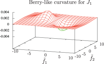
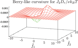
Figure 1: The Berry-like curvatures in $\tilde{f_{1}}-\tilde{f_{2}}$ plane associated with the time-integrated angular velocity $J_{1}$ (Left) and the scaled time-integrated stress tensor $J_{2}D_{r}/\nu k_{B}T$ (Right).

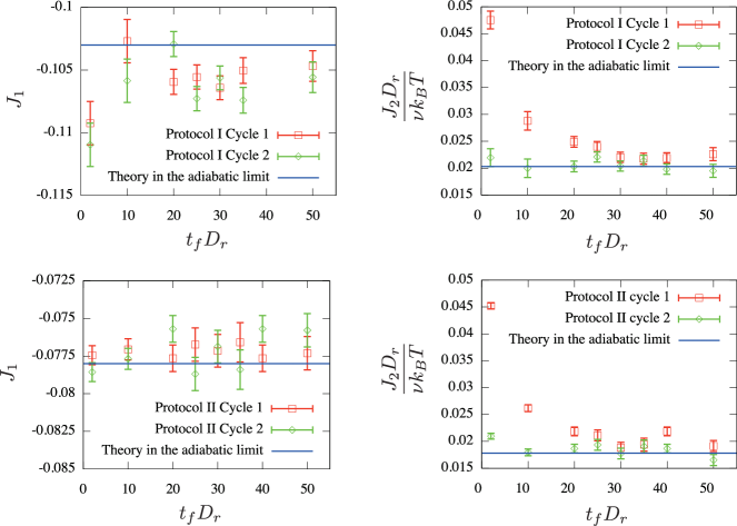
Figure 2: Comparison between the theoretically predicted values and the results of numerical simulations.

V Discussions

In this paper, we have analyzed the Smoluchowski equation under a time-dependent shear. We have found that the time-integrated angular velocity and the time-integrated stress tensor are generated due to the geometrical phase such as Berry-like phase created by an adiabatic modulation of the shear rate even when the housekeeping contributions vanish. It has been shown that the expectation values of the time-integrated angular velocity of a liquid crystalline polymer and the time-integrated stress tensor are generally not zero even if the time average of the shear rate is zero. The validity of our theoretical calculation has been verified by the direct simulation of the Smoluchowski equation. We have confirmed that the theoretically predicted values calculated from the expression obtained in Section III agree well with those obtained by direct numerical simulations of the Smoluchowski equation in adiabatic condition ($t_{f}\rightarrow\infty$).

We can interpret that such excess contributions originates from the deviation of the orientation distribution function from the steady state distribution function as follows. When we modulate the external parameter slowly compared with the rotational diffusion, $\left(\dot{\overleftrightarrow{\kappa}}\left(t\right)\right)$ is proportional to the slowness parameter $\epsilon$. We expect that $F^{\prime}\left(0,\vec{u},t\right)$ can be expanded in terms of $\epsilon$ as

$$F^{\prime}\left(0,\vec{u},t\right)\cong\left(f_{\chi}^{0}\left(\overleftrightarrow{\kappa}\left(t\right),\vec{u}\right)\right)_{\chi=0}+\epsilon\delta F^{\prime}\left(0,\vec{u},t\right)+O\left(\epsilon^{2}\right),$$ (58)

where $\delta F^{\prime}\left(0,\vec{u},t\right)$ is of the order $O\left(1\right)$. Therefore, $\epsilon\delta F^{\prime}\left(0,\vec{u},t\right)$ gives the $O\left(1\right)$ correction to the time-integrated current $J_{i}$ because the required time for a protocol is the order of $O\left(\epsilon^{-1}\right)$.

We examined the dependence of the integrated currents $J_{1}$ and $J_{2}$ on the initial condition. Our results suggest that the dependence of $J_{1}$ on the initial condition is not so strong, which is contrast to the result for a spin-boson system Watanabe hayakawa . The values of $J_{2}$ obtained from the numerical simulations are much larger than the theoretically predicted values if we take the isotropic distribution as an initial condition for $t_{f}\lesssim 25D_{r}^{-1}$, while $J_{2}$ obtained from the numerical simulation agrees well with the theoretical prediction if we adopt the distribution $F^{\prime}\left(0,\vec{u},t_{f}\right)$ obtained numerically as an initial condition. This effect should be regarded as an nonadiabatic effect Watanabe hayakawa because $F^{\prime}\left(0,\vec{u},t_{f}\right)$ approaches to the isotropic distribution in the limit $t_{f}\rightarrow\infty$.

We note that our formulation in Section III for Langevin systems is quite general and applicable to other systems. For example, the motion of a Brownian particle under an adiabatically modulated trapping potential can be discussed within our formulation.

$J_{1}$ can be measured by means of direct observation of the orientation of a rod under shear. However it requires large number of ensembles (about 100000 ensembles even for $t_{f}=2D_{r}^{-1}$ ) in order to reduce the statistical error. $J_{2}$ can be measured by macroscopic rheological experiments on a dilute liquid crystalline solution. In such cases, we expect that it is not needed to make statistical average because there exist large number of liquid crystalline polymers in the solution.

We have discussed the rheology of dilute liquid crystalline solutions, which can be described only by the one-body distribution function of the orientation vectors $\vec{u}$ of rods. It is of interest to investigate whether path-dependent rheological response also exists in other fluid systems where the interactions between particles are important and spatial correlations exist. To investigate such systems, we need to extend our formulation for Liouville equations which describe interacting particle systems or fluctuating hydrodynamic equations.

VI Acknowledgement

One of the authors (S.Y.) was supported by the Japan Society for Promotion of Science. We are grateful to Yusuke Korai for useful discussions and letting us know the formula Eq. (71). This work is partially supported by the Grant-in-Aid of MEXT (Grant No. 25287098).

Appendix A Derivation of Eq. (28)

In this section we derive Eq. (28). At $t=m\epsilon$, we approximate $\frac{dF}{dt}\left(i\chi,\vec{x},t\right)$ as $\frac{dF}{dt}\left(i\chi,\vec{x},t\right)\cong\frac{1}{\epsilon}\left(F_{m}\left(i\chi,\vec{x}\right)-F_{m-1}\left(i\chi,\vec{x}\right)\right)$. Then it can be evaluated as

$$\frac{dF}{dt}\left(i\chi,\vec{x},t\right) \cong \frac{1}{\epsilon}\left(F_{m}\left(i\chi,\vec{x}\right)-F_{m-1}\left(i\chi,\vec{x}\right)\right)$$ (59)

$$= \frac{1}{\epsilon}\left(\frac{1}{\epsilon^{3}}\left(\frac{\epsilon}{4\pi D}\right)^{3/2}\int d^{3}x_{m-1}\exp\left[i\chi\epsilon\left(H\left(\vec{x}_{m-1},\left\{\kappa_{j}\left(\epsilon\left(m-1\right)\right)\right\}\right)\right)\right]\right.$$

$$\left.\times\exp\left[-\frac{\epsilon}{4D}\left(\frac{\vec{x}-\vec{x}_{m-1}}{\epsilon}-\vec{f}\left(\vec{x}_{m-1},\left\{\kappa_{j}\left(\epsilon\left(m-1\right)\right)\right\}\right)\right)^{2}\right]F_{m-1}\left(i\chi,\vec{x}_{m-1}\right)\right)$$

$$-\frac{1}{\epsilon}F_{m-1}\left(i\chi,\vec{x}\right).$$

Here we have used the following relation, which can be derived from the path-integral expression of $F_{m-1}\left(i\chi,\vec{x}_{m-1}\right)$ given by Eq. (24).

$$F_{m}\left(i\chi,\vec{x}\right) = \frac{1}{\epsilon^{3}}\left(\frac{\epsilon}{4\pi D}\right)^{3/2}\int d^{3}x_{m-1}\exp\left[i\chi\epsilon\left(H\left(\vec{x}_{m-1},\left\{\kappa_{j}\left(\epsilon\left(m-1\right)\right)\right\}\right)\right)\right]$$ (60)

$$\times\exp\left[-\frac{\epsilon}{4D}\left(\frac{\vec{x}-\vec{x}_{m-1}}{\epsilon}-\vec{f}\left(\vec{x}_{m-1},\left\{\kappa_{j}\left(\epsilon\left(m-1\right)\right)\right\}\right)\right)^{2}\right]$$

$$\times F_{m-1}\left(i\chi,\vec{x}_{m-1}\right)$$

By expanding $F_{m-1}\left(i\chi,\vec{x}_{m-1}\right)$ around $\vec{x}$:

$$F_{m-1}\left(i\chi,\vec{x}_{m-1}\right)= F_{m-1}\left(i\chi,\vec{x}\right)-\left(\vec{x}-\vec{x}_{m-1}\right)_{k}\frac{\partial}{\partial x_{k}}F_{m-1}\left(i\chi,\vec{x}\right)$$

$$+\frac{1}{2}\left(\vec{x}-\vec{x}_{m-1}\right)_{k}\left(\vec{x}-\vec{x}_{m-1}\right)_{l}\frac{\partial^{2}}{\partial x_{k}\partial x_{l}}F_{m-1}\left(i\chi,\vec{x}\right)+\cdots,$$ (61)

we can derive the following equation in the continuous time limit $\left(\epsilon\rightarrow 0\right)$ by keeping only the terms $O\left(1\right)$.

$$\frac{dF}{dt}\left(i\chi,\vec{x},t\right) \cong \frac{1}{\epsilon}\left(\frac{1}{\epsilon^{3}}\left(\frac{\epsilon}{4\pi D}\right)^{3/2}\int d^{3}x_{m-1}\exp\left[-\frac{\epsilon}{4D}\left(\frac{\vec{x}-\vec{x}_{m-1}}{\epsilon}-\vec{f}\left(\vec{x}_{m-1},\left\{\kappa_{j}\left(\epsilon\left(m-1\right)\right)\right\}\right)\right)^{2}\right]\right.$$ (62)

$$\times\left[1+i\chi\epsilon H\left(\vec{x}_{m-1},\left\{\kappa_{j}\left(\epsilon\left(m-1\right)\right)\right\}\right)+O\left(\epsilon^{2}\right)\right]$$

$$\times\left(F_{m-1}\left(i\chi,\vec{x}\right)-\left(\vec{x}-\vec{x}_{m-1}\right)_{k}\frac{\partial}{\partial x_{k}}F_{m-1}\left(i\chi,\vec{x}\right)\right.$$

$$\left.+\frac{1}{2}\left(\vec{x}-\vec{x}_{m-1}\right)_{k}\left(\vec{x}-\vec{x}_{m-1}\right)_{l}\frac{\partial^{2}}{\partial x_{k}\partial x_{l}}F_{m-1}\left(i\chi,\vec{x}\right)+\cdots\right)$$

$$-\frac{1}{\epsilon}F_{m-1}\left(i\chi,\vec{x}\right)$$

$$= -\left(\vec{f}\left(\vec{x},\left\{\kappa_{j}\left(\epsilon\left(m-1\right)\right)\right\}\right)\right)_{k}\frac{\partial}{\partial x_{k}}F_{m-1}\left(i\chi,\vec{x}\right)+D\nabla^{2}F_{m-1}\left(i\chi,\vec{x}\right)$$

$$-\left(\frac{\partial}{\partial x_{k}}\left(\vec{f}\left(\vec{x},\left\{\kappa_{j}\left(\epsilon\left(m-1\right)\right)\right\}\right)\right)_{k}\right)F_{m-1}\left(i\chi,\vec{x}\right)$$

$$+i\chi H\left(\vec{x},\left\{\kappa_{j}\left(\epsilon\left(m-1\right)\right)\right\}\right)F_{m-1}\left(i\chi,\vec{x}\right)$$

Here we have employed the following equations.

$$\frac{1}{\epsilon}\left(\frac{1}{\epsilon^{3}}\left(\frac{\epsilon}{4\pi D}\right)^{3/2}\int d^{3}x_{m-1}\exp\left[-\frac{\epsilon}{4D}\left(\frac{\vec{x}-\vec{x}_{m-1}}{\epsilon}-\vec{f}\left(\vec{x}_{m-1},\left\{\kappa_{j}\left(\epsilon\left(m-1\right)\right)\right\}\right)\right)^{2}\right]\right.$$

$$= \frac{1}{\epsilon}-\sum_{k}\frac{\partial}{\partial x_{k}}\left(\vec{f}\left(\vec{x},\left\{\kappa_{j}\left(\epsilon\left(m-1\right)\right)\right\}\right)\right)_{k}+O\left(\epsilon\right),$$ (63)

$$\frac{1}{\epsilon}\frac{1}{\epsilon^{3}}\left(\frac{\epsilon}{4\pi D}\right)^{3/2}\int d^{3}x_{m-1}\exp\left[-\frac{\epsilon}{4D}\left(\frac{\vec{x}-\vec{x}_{m-1}}{\epsilon}-\vec{f}\left(\vec{x}_{m-1},\left\{\kappa_{j}\left(\epsilon\left(m-1\right)\right)\right\}\right)\right)^{2}\right]\left(\vec{x}-\vec{x}_{m-1}\right)_{k}$$

$$= \left(\vec{f}\left(\vec{x},\left\{\kappa_{j}\left(\epsilon\left(m-1\right)\right)\right\}\right)\right)_{k}+O\left(\epsilon\right),$$ (64)

$$\frac{1}{\epsilon}\frac{1}{\epsilon^{3}}\left(\frac{\epsilon}{4\pi D}\right)^{3/2}\int d^{3}x_{m-1}\exp\left[-\frac{\epsilon}{4D}\left(\frac{\vec{x}-\vec{x}_{m-1}}{\epsilon}-\vec{f}\left(\vec{x}_{m-1},\left\{\kappa_{j}\left(\epsilon\left(m-1\right)\right)\right\}\right)\right)^{2}\right]$$

$$\times\left(\vec{x}-\vec{x}_{m-1}\right)_{k}\left(\vec{x}-\vec{x}_{m-1}\right)_{l}$$

$$= 2D\delta_{kl}+O\left(\epsilon\right).$$ (65)

Appendix B Several formulae used in the evaluation of the berry-like curvatures

In this section, we give several formulae used in the calculations in Section IV. For $l=1,2,\cdots$ and $m=-l,-l+1,\cdots,l-1,l$ , the spherical harmonics is defined as

$$Y_{lm}\left(\vec{u}\right)=\left(-1\right)^{\left(m+\left|m\right|\right)/2}\sqrt{\frac{2l+1}{4\pi}}\sqrt{\frac{\left(l-\left|m\right|\right)!}{\left(l+\left|m\right|\right)!}}P_{l}^{\left|m\right|}\left(\cos\theta\right)e^{im\phi},$$ (66)

where $P_{l}^{\left|m\right|}$ are associated Legendre polynomials. We note that the polar coordinates $\theta$ and $\phi$ are connected to $\vec{u}$ as

$$\vec{u}=\left(\cos\theta\cos\phi,\cos\theta\sin\phi,\sin\phi\right).$$ (67)

The matrix representations of $\mathcal{K}_{0}^{\prime}$ and $H_{i}$ for $i=1,2$ are given by

$$\left\langle lm\left|\mathcal{K}_{0}^{\prime}\right|l^{\prime}m^{\prime}\right\rangle$$

$$= -l\left(l+1\right)\delta_{ll^{\prime}}\delta_{mm^{\prime}}$$

$$-\frac{1}{3}\sqrt{\frac{\left(2l^{\prime}+1\right)}{\left(2l+1\right)}}\left\langle l,0\left|2,0,\right.l^{\prime}0\right\rangle\times$$

$$\left[\left(f_{1}-if_{2}\right)\sqrt{l\left(l+1\right)-\left(m-1\right)m}\left\langle l,\left(m-1\right)\left|2,0,\right.l^{\prime}m^{\prime}\right\rangle\right.$$

$$\left.+\left(-f_{1}-if_{2}\right)\sqrt{l\left(l+1\right)-\left(m+1\right)m}\left\langle l,\left(m+1\right)\left|2,0,\right.l^{\prime}m^{\prime}\right\rangle\right]$$

$$+\left(-f_{1}+if_{2}\right)\frac{1}{6}\sqrt{l\left(l+1\right)-\left(m-1\right)m}\delta_{m-1,m^{\prime}}\delta_{l,l^{\prime}}$$

$$+\left(f_{1}+if_{2}\right)\frac{1}{6}\sqrt{l\left(l+1\right)-\left(m+1\right)m}\delta_{m+1,m^{\prime}}\delta_{l,l^{\prime}}$$

$$+m\left\langle l,0\left|2,0,\right.l^{\prime}0\right\rangle\sqrt{\frac{\left(2l^{\prime}+1\right)}{6\left(2l+1\right)}}$$

$$\times\left(\left(-f_{1}+if_{2}\right)\left\langle l,m\left|2,1,\right.l^{\prime}m^{\prime}\right\rangle+\left(-f_{1}-if_{2}\right)\left\langle l,m\left|2,-1,\right.l^{\prime}m^{\prime}\right\rangle\right),$$ (68)

$$\left\langle lm\left|H_{1}\right|l^{\prime}m^{\prime}\right\rangle=-f_{2}\frac{1}{3}\left(2\sqrt{\frac{\left(2l^{\prime}+1\right)}{\left(2l+1\right)}}\left\langle l,0\left|2,0,\right.l^{\prime}0\right\rangle\left\langle l,m\left|2,0,\right.l^{\prime}m^{\prime}\right\rangle+\delta_{ll^{\prime}}\delta_{mm^{\prime}}\right),$$ (69)

$$\left\langle lm\left|H_{2}\right|l^{\prime}m^{\prime}\right\rangle$$

$$= \sqrt{\frac{\left(2l^{\prime}+1\right)}{\left(2l+1\right)}}\times$$

$$\left[\left\langle l,0\left|4,0,\right.l^{\prime}0\right\rangle\times\left(-\frac{1}{7\sqrt{10}}\left(if_{1}+f_{2}\right)\left\langle l,m\left|4,2,\right.l^{\prime},m^{\prime}\right\rangle\right.\right.$$

$$\left.+\frac{1}{7\sqrt{10}}\left(if_{1}-f_{2}\right)\left\langle l,m\left|4,-2,\right.l^{\prime},m^{\prime}\right\rangle-\frac{2}{35}f_{1}\left\langle l,m\left|4,0,\right.l^{\prime},m^{\prime}\right\rangle\right)$$

$$+\left\langle l,0\left|2,0,\right.l^{\prime}0\right\rangle\times$$

$$\left(\frac{1}{14}\sqrt{\frac{1}{6}}\left(-if_{1}-f_{2}\right)\left\langle l,m\left|2,2,\right.l^{\prime},m^{\prime}\right\rangle+\sqrt{\frac{3}{2}}i\left\langle l,m\left|2,1,\right.l^{\prime},m^{\prime}\right\rangle\right.$$

$$+\frac{1}{42}f_{2}\left\langle l,m\left|2,0,\right.l^{\prime},m^{\prime}\right\rangle+\sqrt{\frac{3}{2}}i\left\langle l,m\left|2,-1,\right.l^{\prime},m^{\prime}\right\rangle$$

$$\left.+\frac{1}{14}\sqrt{\frac{1}{6}}\left(if_{1}-f_{2}\right)\left\langle l,m\left|2,-2,\right.l^{\prime},m^{\prime}\right\rangle\right)$$

$$\left.+\frac{1}{30}f_{2}\delta_{ll^{\prime}}\delta_{mm^{\prime}}\right].$$ (70)

Here we have employed the Dirac’s bra-ket notation and $\left|l,m\right\rangle$ represents $Y_{lm}\left(\vec{u}\right)$. We have also introduced the Clebsch-Gordan coefficients $\left\langle l,m\left|l^{\prime}m^{\prime},\right.l^{\prime\prime}m^{\prime\prime}\right\rangle$. In deriving these expressions, we have used the following formula Messiah .

$$\int d\Omega\left(Y_{lm}\left(\vec{u}\right)\right)^{*}Y_{l_{1}m_{1}}\left(\vec{u}\right)Y_{l_{2}m_{2}}\left(\vec{u}\right)$$

$$= \sqrt{\frac{\left(2l_{1}+1\right)\left(2l_{2}+1\right)}{4\pi\left(2l+1\right)}}\left\langle l0\left|l_{1}0,\right.l_{2}0\right\rangle\left\langle lm\left|l_{1}m_{1},\right.l_{2}m_{2}\right\rangle$$ (71)

References

- (1) M. V. Berry, Proc. Roy. Soc. Lond. A 392, 45 (1984).
- (2) J. Samuel and R. Bhandari, Phys. Rev. Lett. 60, 2339 (1988).
- (3) D. J. Thouless, Phys. Rev. B 27, 6083 (1983).
- (4) N. A. Sinitsyn and I. Nemenman, Europhys. Lett. 77, 58001 (2007).
- (5) N. A. Sinitsyn and I. Nemenman, Phys. Rev. Lett. 99, 220408 (2007).
- (6) J. Ohkubo, J. Chem. Phys. 129, 205102 (2008).
- (7) V. Y. Chernyak, J. R. Klein, and N. A. Sinitsyn, J. Chem. Phys. 136, 154107 (2012), ibid 154108 (2012).
- (8) T. Sagawa and H. Hayakawa, Phys. Rev. E 84, 051110 (2011).
- (9) J. Ren, P. Hänggi, and B. Li, Phys. Rev. Lett. 104, 170601 (2010).
- (10) T. Yuge, T. Sagawa, A. Sugita, and H. Hayakawa, Phys. Rev. B 86, 235308 (2012).
- (11) K. L. Watanabe and H. Hayakawa, Prog. Theor. Exp. Phys. 113A01 (2014).
- (12) M. Doi and S. F. Edwards, The theory of polymer dynamics, (Oxford university press, Oxford, 1988).
- (13) P. G. de Gennes and J. Prost, The Physics of Liquid Crystals, Clarendon Press, Oxford, 2nd edn, 1993.
- (14) N. Nemoto, J. L. Schrag, J. D. Ferry, and R. W. Fulton, Biopolymers 14, 409 (1975).
- (15) N. Ookubo, M. Komatsubara, H. Nakajima, and Y. Wada, Biopolymers 15 929 (1976).
- (16) M. Harasim, B. Wunderlich, O. Peleg, M. Kröger, and A. R. Bausch, Phys. Rev Lett. 110 (2013) 108302.
- (17) J. M. J. van Leeuwen, H. W. J. Blöte, arXiv:1406.1317.
- (18) E. J. Hinch and L. G. Leal, Fluid Mech. 52, 683 (1972).
- (19) E. J. Hinch and L. G. Leal, Fluid Mech. 76, 187 (1976).
- (20) W. E. Stewart and J. P. Sorensen, Trans. Soc. Rheol. 16, 1 (1972).
- (21) N. A. Sinitsyn, J. Phys. A: Math. Theor. 42 193001 (2009).
- (22) J. Ohkubo, IEICE Transactions on Communications, E96-B 11 2733 (2013).
- (23) A. Messiah, Quantum Mechanics, (Dover Publications, New York 2014).