Minimum Local Distance Density Estimation

Abstract

We present a local density estimator based on first order statistics. To estimate the density at a point, $x$, the original sample is divided into subsets and the average minimum sample distance to $x$ over all such subsets is used to define the density estimate at $x$. The tuning parameter is thus the number of subsets instead of the typical bandwidth of kernel or histogram-based density estimators. The proposed method is similar to nearest-neighbor density estimators but it provides smoother estimates. We derive the asymptotic distribution of this minimum sample distance statistic to study globally optimal values for the number and size of the subsets. Simulations are used to illustrate and compare the convergence properties of the estimator. The results show that the method provides good estimates of a wide variety of densities without changes of the tuning parameter, and that it offers competitive convergence performance.

Keywords: Density estimation, nearest-neighbor, order statistics

1 Introduction

Nonparametric density estimation is a classic problem that continues to play an important role in applied statistics and data analysis. More recently, it has also become a topic of much interest in computational mathematics, especially in the uncertainty quantification community where one is interested in, for example, densities of a large number of coefficients of a random function in terms of a fixed set of deterministic functions (e.g., truncated Karhunen-Loève expansions). The method we present here was motivated by such applications.

Among the most popular techniques for density estimation are the histogram [Scott, 1979, Scott, 1992], kernel [Parzen, 1962, Scott, 1992, Wand and Jones, 1995] and orthogonal series [Efromovich, 2010, Silverman, 1986] estimators. For the one-dimensional case, histogram methods remain in widespread use due to their simplicity and intuitive nature, but kernel density estimation has emerged as a method of choice thanks, in part, to recent adaptive bandwidth-selection methods providing fast and accurate results [Botev et al., 2010]. However, these kernel density estimators can fail to converge in some cases (e.g., recovering a Cauchy density with Gaussian kernels) [Buch-Larsen et al., 2005] and can be computationally expensive with large samples (${{\cal O}\left(N^{2}\right)}$, for a sample size $N$). Note that histogram estimators are typically implemented using equal-sized bins, and nearest-neighbor density estimators can be roughly thought as histograms whose bins adapt to the local density of the data. More precisely, let $X_{1},\ldots,X_{N}$ be iid variables from a distribution with density, $f$, and let $X_{(1)},\ldots,X_{(N)}$ be the corresponding order statistics. For any $x$, define $Y_{i}=|X_{i}-x|$ and $D_{j}(x)=Y_{(j)}$. The $k$-nearest-neighbor estimate of $f$ is defined as (see [Silverman, 1986] for an overview): $\widehat{f}_{N}(x)=(\,C_{N}/N\,)/[\,2D_{k}(x)\,],$ where $C_{N}$ is a constant that may depend on the sample size. We may think of $2D_{k}(x)$ as the width of the bin around $x$. The value of $C_{N}$ is often chosen as $C_{N}\approx N^{1/2}$ but some effort has been directed towards its optimal selection [Fukunaga and Hostetler, 1973, Hall et al., 2008, Li, 1984], with some recent work involving the use of order statistics [Kung et al., 2012]. One of the disadvantages of nearest-neighbor estimators is that their derivative has discontinuities at the points $(X_{(j)}+X_{(j+k)})/2$, which is caused by the discontinuities of the derivative of the function $D_{k}(x)$ at these points. This is clear in Figure 1, which shows plots of $D_{k}(x)$ for a sample of size $N=125$ from a Cauchy$(0,1)$ distribution with $k=1$ and $k=round(\sqrt{N})$. One way to obtain smoother densities is using a combination of kernel and nearest-neighbor density estimation where the nearest-neighbors technique is used to choose the kernel bandwidth [Silverman, 1986]. We introduce an alternative averaging method that improves smoothness and can still be used to obtain local density estimates.

The main idea of this paper may be summarized as follows: Instead of using the $k$th nearest-neighbor to provide an estimate of the density at a point, $x$, we use a subset-average of first order statistics of $|X_{i}-x|$. So, the original sample of size $N$ is split into $m$ subsets of size $s$ each; this decomposition into subsets allows the control of the asymptotic mean squared error (MSE) of the density estimate. Thus, the problem of bandwidth selection is transformed into that of choosing an optimal number of subsets. This density estimator is naturally parellelizable with complexity ${{\cal O}\left(N^{{1}/{3}}\right)}$ for parallel systems.

The rest of this article is organized as follows. In Section 2 we develop the theory that underlies the estimator and describe asymptotic results. In Sections 3 and 4 we describe the actual estimator and study its performance using numerical experiments. A variety of densities are used to reveal the strengths and weaknesses of the estimator. We provide concluding remarks and generalizations in Section 5. Proofs and other auxiliary results are collected in Appendix A. From here on, when we refer to the size of a sample set being the power of the total number of samples, we assume that it represents a rounded value, for example, $k=\sqrt{N}\Rightarrow k=round(\sqrt{N})$.

2 Theoretical framework

Let $X_{1},\ldots,X_{N}$ be iid random variables from a distribution with invertible CDF, $F$, and PDF $f$. Our goal is to estimate the value of $f$ at a point, $x_{*}$, where $f(x_{*})>0$, and where $f$ is either continuous or has a jump discontinuity. The non-negative random variables $Y_{i}=|X_{i}-x_{*}|$ are iid with PDF: $g(y)=f(y+x_{*})+f(x_{*}-y).$ In particular, $f(x_{*})=g(0)/2$. Thus, an estimate of $g(0)$ leads to an estimate of $f(x_{*})$. Furthermore, $g$ is more regular than $f$ in a sense described by the following lemma (its proof and those of the other results in this section are collected in Appendix A).

Lemma 1.

Let $f$ and $g$ be as defined above. Then:

• If $f$ has left and right limits at $x_{*}$ (i.e., it is either continuous or has a jump discontinuity at $x_{*}$), then $g$ is continuous at zero.

• If $f$ has left and right derivatives at $x_{*}$, then $g$ has a right derivative at zero. Furthermore, if $f$ is differentiable at $x_{*}$, then $g^{\prime}(0)=0$.

The original question is thus reduced to the following problem: Let $X_{1},\ldots,X_{N}$ be iid non-negative random variables from a distribution with invertible CDF, $G$, and PDF $g$. The goal is to estimate $g(0)>0$ assuming that $g$ is right continuous at zero. The continuity at zero comes from Lemma 1(i). For some asymptotic results we also assume that $g$ is right-differentiable with $g^{\prime}(0)=0$. The zero derivative is justified by Lemma 1(ii). We estimate $g(0)$ using a subset-average of first order statistics.

There is a natural connection between density estimation and first order statistics: If ${X_{(1),N}}$ is the first order statistic of $X_{1},\ldots,X_{N}$, then (under regularity conditions) $\mathbb{E}{X_{(1),N}}\sim Q(1/(N+1))$ as $N\to\infty$, where $Q=G^{-1}$ is the quantile function, and therefore $(N+1)\,\mathbb{E}{X_{(1),N}}\to 1/g(0)$. This shows that one should be able to estimate $g(0)$ provided $N$ is large and we have a consistent estimate of $\mathbb{E}{X_{(1),N}}$. In the next section we provide conditions for the limit to be valid and derive a similar limit for the second moment of ${X_{(1),N}}$; we then define the estimator and study its asymptotics.

2.1 Limits of first order statistics

We start by finding a representation of the first two moments of the first-order statistic in terms of functions that allow us to determine the limits of the moments as $N\to\infty$.

Lemma 2.

Let $X_{1},\ldots,X_{N}$ be iid non-negative random variables with PDF $g$, invertible CDF $G$ and quantile function $Q$. Assume that $g(0)>0$, and define the sequence of functions $\delta_{N}(z)=(N+1)(1-z)^{N}$ on $z\in[0,1]$, $N\in\mathbb{N}$. Then:

• $$(N+1)\,\mathbb{E}{X_{(1),N}} = \int_{0}^{1}\frac{\delta_{N}(z)}{g(Q(z))}\,dz=\int_{0}^{1}Q^{\prime}(z)\,\delta_{N}(z)\,dz$$ (1)

  $$= \frac{1}{g(0)}+\frac{1}{(N+2)}\int_{0}^{1}Q^{\prime\prime}(z)\,\delta_{N+1}(z)\,dz.$$ (2)

  Furthermore, if $g$ is twice differentiable with $g^{\prime}(0)=0$, then

  $$(N+1)\,\mathbb{E}{X_{(1),N}}=\frac{1}{g(0)}+\frac{1}{(N+2)(N+3)}\int_{0}^{1}Q^{\prime\prime\prime}(z)\,\delta_{N+2}(z)\,dz.$$ (3)

• If $g$ is differentiable a.e., then

  $$(N+1)^{2}\,\mathbb{E}[\,{X_{(1),N}}^{2}\,]=\left(\frac{N+1}{N+2}\right)\int_{0}^{1}(Q^{2}(z))^{\prime\prime}\,\delta_{N+1}(z)\,dz.$$ (4)

We use the following result to evaluate the limits of the moments as $N\to\infty$.

Proposition 2.1.

Let $H$ be a function defined on $[0,1]$ that is continuous at zero, and assume there is an integer $m>0$ and a constant $C>0$ such that

$$|H(x)|\leq{C}/{(1-x)^{m}}$$ (5)

a.e. on $[0,1]$. Then,  $\lim_{N\to\infty}\int_{0}^{1}H(x)\,\delta_{N}(x)\,dx=H(0).$

This proposition allows us to compute the limits of (1)-(4) provided the quantile functions satisfy appropriate regularity conditions. When a function $H$ satisfies (5), we shall say that $H$ satisfies a tail condition for some $C>0$ and integer $m>0$. The following corollary follows from Lemma 2 and Proposition 2.1:

Corollary 1.

Let $X_{1},\ldots,X_{N}$ be iid non-negative random variables with PDF $g$, invertible CDF $G$ and quantile function $Q$. Assume that $g(0)>0$. Then:

If $g$ is continuous at zero and $Q^{\prime}$ satisfies a tail condition, then

$$\lim_{N\to\infty}(N+1)\,\mathbb{E}{X_{(1),N}}=Q^{\prime}(0)={1}/{g(0)}.$$ (6)

If $g$ is differentiable and $Q^{\prime\prime}$ satisfies a tail condition, then

$$(N+1)\,\mathbb{E}{X_{(1),N}}={1}/{g(0)}+{{\cal O}\left(1/N\right)}.$$ (7)

If $g$ is twice differentiable with $g^{\prime}(0)=0$, $g^{\prime\prime}$ is continuous at zero and $Q^{\prime\prime\prime}$ satisfies a tail condition, then

$$(N+1)\,\mathbb{E}{X_{(1),N}}={1}/{g(0)}+{{\cal O}\left(1/N^{2}\right)}.$$ (8)

If $g$ is differentiable a.e., $g^{\prime}$ and $g$ are continuous at zero, and $Q^{\prime\prime}$ satisfies a tail condition, then

$$\lim_{N\to\infty}(N+1)^{2}\,\mathbb{E}[{X_{(1),N}}^{2}] = 2\,Q^{\prime}(0)^{2}={2}/{g(0)^{2}}$$ (9)

$$\lim_{N\to\infty}{\mathbb{V}{\rm ar}}\left[\,(N+1)\,{X_{(1),N}}\,\right] = {1}/{g(0)^{2}}.$$ (10)

We now provide examples of distributions that satisfy the hypotheses of Corollary 1. For these examples, we temporarily return to the notations $X_{i}$ (iid random variables) and $Y_{i}=|X_{i}-x_{*}|$ used before Lemma 1.

Example 1.

Let $X_{1},\ldots,X_{N}$ be iid with exponential distribution $\mathcal{E}(\lambda)$ and fix $x_{*}>0$. The PDF, CDF and quantile function of $Y_{i}$ are, respectively,

$$g(y) = 2\lambda\,e^{-\lambda x_{*}}\cosh(\lambda y)\,I_{y\leq x_{*}}+\lambda\,e^{-\lambda(x_{*}+y)}\,I_{y>x_{*}}$$

$$G(y) = 2e^{-\lambda x_{*}}\sinh(\lambda y)\,I_{y\leq x_{*}}+(1-e^{-\lambda(x_{*}+y)})\,I_{y>x_{*}}$$

$$Q(z) = \lambda^{-1}\mathrm{arcsinh}(ze^{\lambda x_{*}}/2)\,I_{z\leq z_{*}}-[\,x_{*}+\lambda^{-1}\,\log(1-z)\,]\,I_{z>z_{*}}$$

for $y\geq 0$, $z\in[0,1)$ and $z_{*}=1-e^{-2\lambda x_{*}}$. As expected, $g^{\prime}(0)=0$. In addition, $Q$ and its derivatives are continuous at zero. Furthermore, since $|\log(1-z)|\leq z/(1-z)$ on $(0,1)$, we see that $Q$ and its derivatives satisfy tail conditions.

Example 2.

Let $X_{1},\ldots,X_{N}$ be iid with Cauchy distribution and fix $x_{*}\in{\mathbb{R}}$. The PDF and CDF of $Y_{i}$ are:

$$g(y) = \frac{1}{\pi[1+(y+x_{*})^{2}]}+\frac{1}{\pi[1+(x_{*}-y)^{2}]}$$

$$G(y) = \arctan(y+x_{*})/\pi-\arctan(x_{*}-y)/\pi.$$

Again, $g^{\prime}(0)=0$. To verify the conditions on the quantile function, $Q$, note that

$$Q(z)=-\cot(\pi z)+\cot(\pi z)\sqrt{1+(1+x_{*}^{2})\tan^{2}(\pi z)},$$

in a neighborhood of zero, while for $z$ in a neighborhood of 1, $Q$ is given by

$$Q(z)=-\cot(\pi z)-\cot(\pi z)\sqrt{1+(1+x_{*}^{2})\tan^{2}(\pi z)}.$$

Since $Q(z)\to 0$ as $z\to 0^{+}$ and $g$ is smooth, it follows that $Q$ and its derivatives are continuous at zero. It is easy to see that the tail conditions for $Q^{\prime}$, $Q^{\prime\prime\prime}$ and $(Q^{2})^{\prime\prime}$ are determined by the tail condition of $\csc(\pi z)$, which in turn follows from the inequality $|\csc(\pi z)|\leq 1/[\,\pi z(1-z)]$ on $(0,1)$.

It is also easy to check that the Gaussian and beta distributions satisfy appropriate tail conditions for Corollary 1.

2.2 Estimators and their properties

Let $X_{1},\ldots,X_{N}$ be iid non-negative random variables whose PDF $g$, CDF $G$ and quantile function $Q$ satisfy appropriate regularity conditions for Corollary 1. We randomly split the sample into $m_{N}$ independent subsets of size $s_{N}$. Both sequences, $(m_{N})$ and $(s_{N})$, tend to infinity as $N\to\infty$ and satisfy $m_{N}s_{N}=N$. Let $X^{(1)}_{(1),s_{N}},\ldots,X^{(m_{N})}_{(1),s_{N}}$ be the first-order statistics for each of the $m_{N}$ subsets, and let ${\overline{X}_{m_{N},s_{N}}}$ be their average,

$${\overline{X}_{m_{N},s_{N}}}=\frac{1}{m_{N}}\sum_{k=1}^{m_{N}}X^{(k)}_{(1),s_{N}}.$$ (11)

The estimators of $1/g(0)$ and $g(0)$ are defined, respectively, as:

$$\widehat{f^{-1}(0)}_{N}=(s_{N}+1){\overline{X}_{m_{N},s_{N}}},\quad\widehat{f(0)}_{N}=1/\widehat{f^{-1}(0)}_{N}.$$ (12)

Proposition 2.2.

Let $N$, $m_{N}$ and $s_{N}$ be as defined above. Then:

• If $g$ is differentiable a.e., $g^{\prime}$ and $g$ are continuous at zero, and $Q^{\prime\prime}$ satisfies a tail condition, then

  $$\lim_{N\to\infty}{\rm MSE}(\,\widehat{f^{-1}(0)}_{N}\,)=0,$$ (13)

  and therefore $\widehat{f(0)}_{N}\stackrel{{\scriptstyle{P}}}{{\longrightarrow}}g(0)$ as $N\to\infty$.

• Let $g$ be twice differentiable with $g^{\prime}(0)=0$, $g^{\prime\prime}$ be continuous at zero, and let $Q^{\prime\prime\prime}$ satisfy a tail condition. If $\sqrt{m_{N}}/s_{N}\to\infty$ and $\sqrt{m_{N}}/s_{N}^{2}\to 0$ as $N\to\infty$, then

  $$\sqrt{m_{N}}\left(\,\widehat{f^{-1}(0)}_{N}-1/g(0)\,\right)\stackrel{{\scriptstyle{\cal L}}}{{\longrightarrow}}N(0,1/g(0)^{2}),$$ (14)

  which leads to

  $$\sqrt{m_{N}}\left(\,\widehat{f(0)}_{N}-g(0)\,\right)\stackrel{{\scriptstyle{\cal L}}}{{\longrightarrow}}N(0,g(0)^{2}).$$ (15)

  Furthermore, ${\rm MSE}(\widehat{f^{-1}(0)}_{N})$ and ${\rm MSE}(\widehat{f(0)}_{N})$ are ${{\cal O}\left(1/m_{N}\right)}$. In particular, (14) and (15) are satisfied when $s_{N}=N^{\alpha}$ and $m_{N}=N^{1-\alpha}$ for some $\alpha\in(1/5,1/3)$. This leads to the MSE optimal rate ${{\cal O}\left(N^{-4/5-\varepsilon}\right)}$ for any $\varepsilon>0$.

By (ii), we need a balance between the sample size, $s_{N}$, and the number of samples, $m_{N}$: $m_{N}$ should grow faster than $s_{N}$ but not much faster. For comparison, the optimal rate of the MSE is ${{\cal O}\left(N^{-2/3}\right)}$ for the smoothed histogram, and ${{\cal O}\left(N^{-4/5}\right)}$ for the kernel density estimator [DasGupta, 2008].

Distance function

We return to the original sample $X_{1},\ldots,X_{N}$ from a density $f$ before the transformation to $Y_{1}=|X_{1}-x|,\ldots,Y_{N}=|X_{N}-x|$. The sample is split into $m_{N}$ subsets. Let $D_{1}(x;m)$ be the distance from $x$ to its nearest-neighbor in the $m$th subset. The mean ${\overline{X}_{m_{N},s_{N}}}$ in (11) is the average of $D_{1}(x;m)$ over all the subsets; we call this average the distance function, $D_{\rm MLD}$, of the MLD density estimator. That is,

$$D_{\rm MLD}(x)={\overline{X}_{m_{N},s_{N}}}=\frac{1}{m_{N}}\sum_{m=1}^{m_{N}}D_{1}(x;m).$$

The estimators in (12) can then be written in terms of $D_{\rm MLD}(x)$. This distance function tends to be smoother than the usual distance function used by $k$-nearest-neighbor density estimators. For example, Figure 1 shows the different distance functions $D_{\rm MLD}(x)$, $D_{1}(x)$ and $D_{k}(x)$ (the latter as defined in the introduction) for a sample of $N=125$ variables from a Cauchy$(0,1)$. Note that $D_{\rm MLD}$ is an average of first-order statistics for samples of size $s_{N}$, while $D_{1}$ is a first-order statistic for a samples of size $N$, so $D_{\rm MLD}>D_{1}$. On the other hand, $D_{\sqrt{N}}$ is a $N^{1/2}$th-order statistic based on a sample of size $N$; hence the order $D_{\rm MLD}>D_{\sqrt{N}}>D_{1}$.

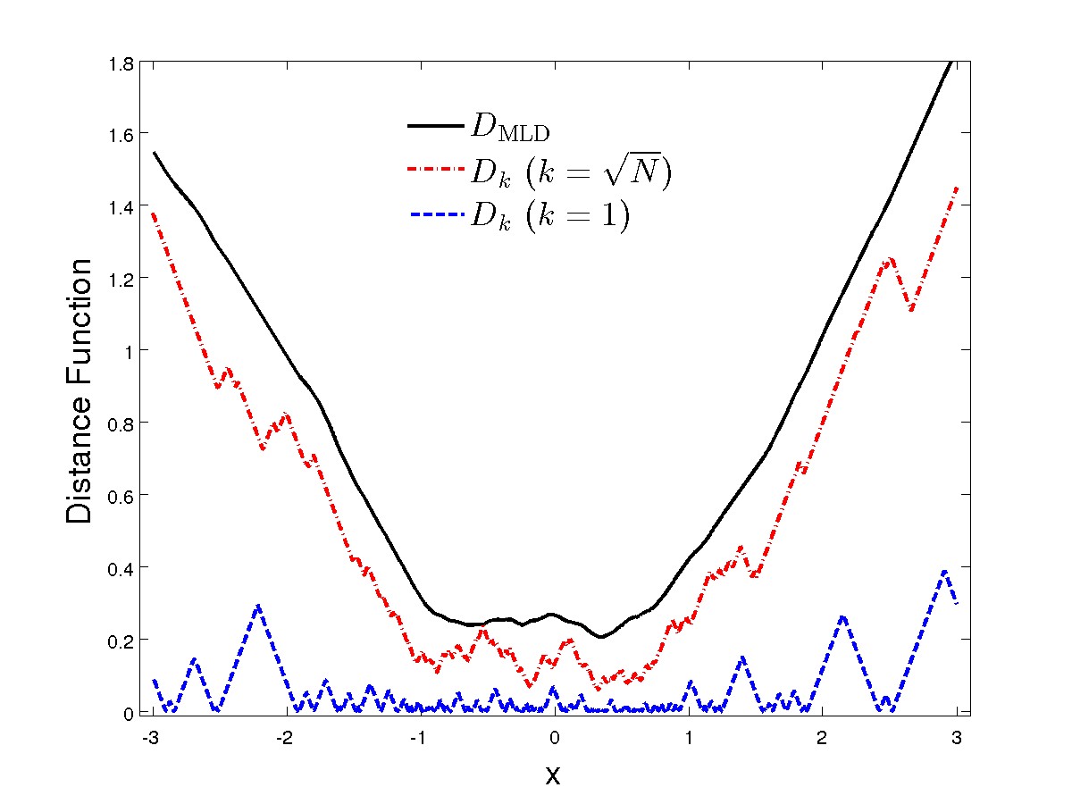
Figure 1: Distance function $D_{k}(x)$ for $k$-nearest-neighbor (for $k=1$ and $k=11\approx\sqrt{N}$) and the distance function $D_{\rm MLD}(x)$ (with $m_{N}=N^{\frac{2}{3}}=25$ subsets) for 125 samples taken from a Cauchy(0,1) distribution.

3 Minimum local distance density estimator

We now describe the local distance density estimator (MLD-DE). The inputs are: a sample, a set of points where the density is to be estimated and the parameter $\alpha$ whose default is set to $\alpha=1/3$. The basic steps to obtain the density estimate at a point $x$ are: (1) Start with a sample of $N$ iid variables from the unknown density, $f$; (2) Randomly split the sample into $m_{N}=N^{1-\alpha}$ disjoint subsets of size $s_{N}=N^{\alpha}$ each; (3) Find the nearest sample distance to $x$ in each subset; (4) Compute the density estimate by inverting the average nearest distance across the subsets and scaling it (see Eq.(12)). This is summarized in Algorithm 1.

Algorithm 1 Returns density estimates at the points of evaluation $\{x_{l}\}_{l=1}^{M}$ given the sample $X_{1},\ldots,X_{N}$ from the unknown density $f$.

1:$m_{N}\leftarrow$ round($N^{1-a}$)

2:$s_{N}\leftarrow$ round(${N}/{m_{N}}$)

3:Create an $s_{N}\times m_{N}$ matrix $M_{ij}$ with the $m_{N}$ subsets with $s_{N}$ variables each

4:Create a vector $\widehat{f}=(\widehat{f}_{\ell})$ to hold the density estimates at the points $\{x_{l}\}_{l=1}^{M}$

5:for $l=1\to M$ do

6:     for $k=1\to s_{N}$ do

7:         Find the nearest distance $d_{lk}$ to the current point $x_{\ell}$ within the $k$th subset

8:     end for

9:     Compute the subset average of distances to $x_{\ell}$: $d_{\ell}=(1/m_{N})\sum\limits_{k=1}^{m_{N}}d_{\ell k}$

10:     Compute the density estimate at $x_{l}$: $\widehat{f}_{\ell}={1}/{2d_{\ell}}$

11:end for

12:return $\widehat{f}$

Note that for each of the $M$ points where the density is to be estimated, the algorithm loops over $N^{1-\alpha}$ subsets, and within each it does a nearest-neighbor search over $N^{\alpha}$ points. The computational complexity is therefore ${{\cal O}\left(MN^{1-\alpha}N^{\alpha}\right)}={{\cal O}\left(MN\right)}$, which is of the same order as the ${{\cal O}\left(N^{2}\right)}$ complexity of kernel density estimators [Raykar et al., 2010] when $M\sim N$. However, MLD-DE displays multiple levels of parallelism. The first level is the highly parallelizable evaluation of the density at the $M$ specified points. The second level arises from the the nearest-neighbor distances that can be computed independently in each subset. Thus, for parallel systems the effective computational complexity of the algorithm is ${{\cal O}\left(MN^{\alpha}\right)}$, which is the same as that of histogram methods if $\alpha={1}/{3}$.

4 Numerical examples

An extensive suite of numerical experiments was used to test the MLD-DE method. We now summarize the results to show that they are consistent with the theory derived in Section 2, and illustrate some salient features of the estimator. We also compare MLD-DE to the adaptive kernel density estimator (KDE) introduced by Botev et al. [Botev et al., 2010] and to the histogram method based on Scott’s normal reference rule [Scott, 1979].

We first discuss experiments for density estimation at a fixed point and show the effects of changing the number of subsets for a fixed sample size. We then estimate the integrated mean square error for various densities, and compare the convergence of MLD-DE to that of other density estimators. Next, we present numerical experiments that show the spatial variation of the bias and variance of MLD-DE, and relate them to the theory derived in Section 2. Finally, we check the impact of changing the tuning parameter $\alpha$ (see Proposition 2.2).

4.1 Pointwise estimation of a density

We use MLD-DE to estimate values of the beta$(1,4)$ and $N(0,1)$ densities at a single point and analyze its convergence performance. Starting with a sample size $N=100$, $N$ was progressively increased to three million. For each $N$, 1000 trials were performed to estimate the MSE of the density estimate. The parameter $\alpha$ was also changed; it was set to ${1}/{3}$ for one set of experiments anticipating a bias of ${{\cal O}\left({1}/{N}\right)}$, and to ${1}/{5}$ for another set, anticipating a bias of ${{\cal O}\left({1}/{N^{2}}\right)}$. The results are shown in Figure 2.

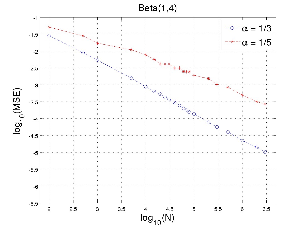
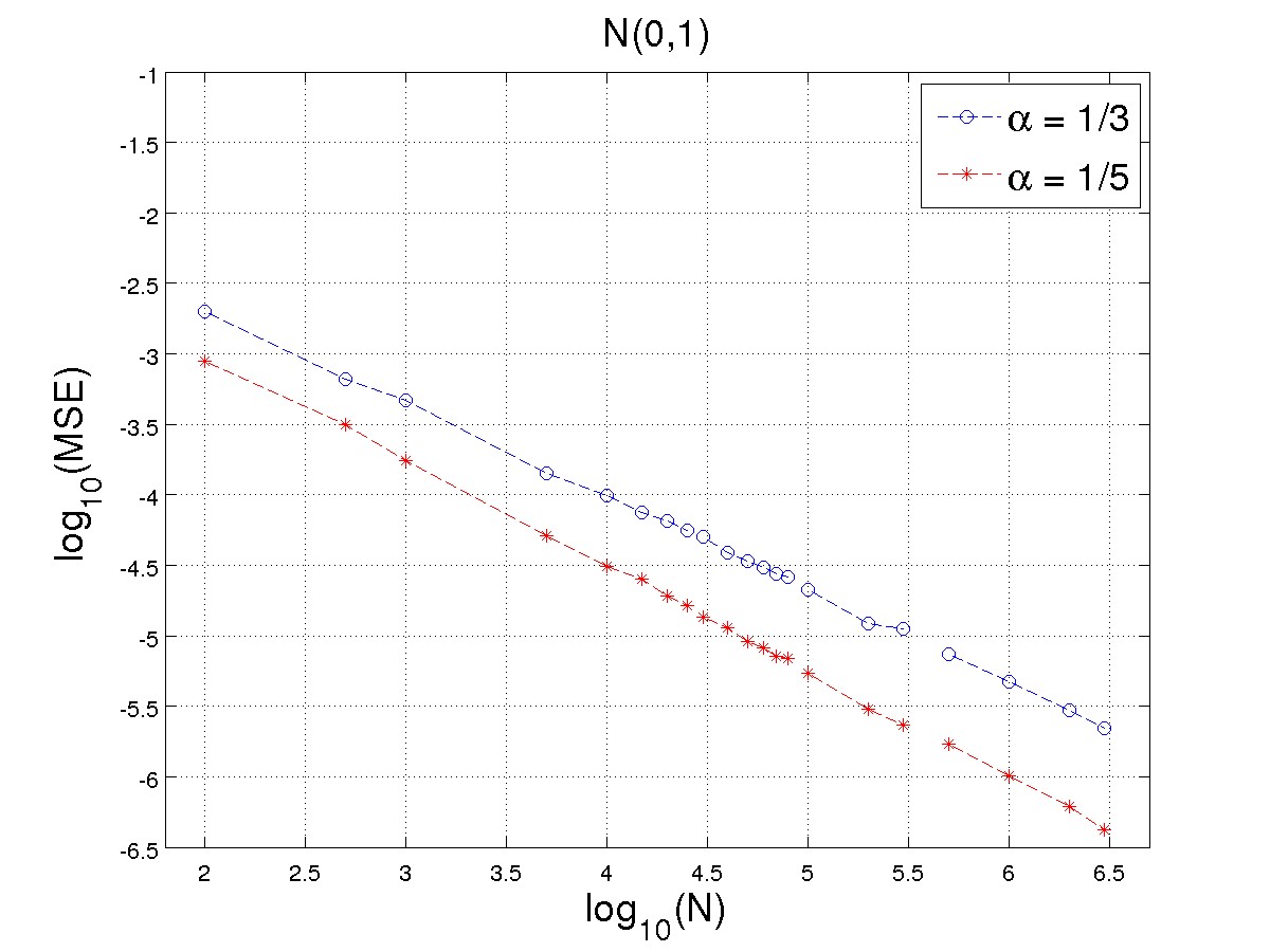
Figure 2: Convergence plots of the density estimates at $x=1/2$ for the distribution beta$(1,4)$ (left), and at $x=1$ for $N(0,1)$ (right).

We see the contrasting convergence behavior for the beta$(1,4)$ and $N(0,1)$ distributions. For the former, the convergence is faster when $\alpha={1}/{3}$, while for the Gaussian it is faster with $\alpha={1}/{5}$. We recall from Section 2 that the asymptotic bias of the density estimate at a point is ${{\cal O}\left({1}/{N^{2}}\right)}$. However, reaching the asymptotic regime depends on the convergence of $\int_{0}^{1}Q^{\prime\prime}(z)\,\delta_{N}(z)\,dz$ to zero, which can be quite slow, depending on the behavior of the density at the chosen point. Hence, the effective bias in simulations can be ${{\cal O}\left({1}/{N}\right)}$. The numerical experiments thus indicate that the quantile function derivative of the Gaussian decays to zero much faster than that of the beta distribution, and hence the optimal value of $\alpha$ for $N(0,1)$ is ${1}/{5}$, while that for beta$(1,4)$ is ${1}/{3}$. However, in either case the order of the decay in the figure is close to $N^{-3/4}$.

4.2 $L^{2}$-convergence

We now summarize simulation results regarding the $L^{2}$-error (i.e., integrated MSE) of estimates of a beta$(1,4)$, a Gaussian mixture and the Cauchy$(0,1)$ density. The Gaussian mixture used is (see  [Wasserman, 2006]): $0.5\,N(0,1)+0.1\sum_{i=0}^{4}N(\,i/2-1,\,1/100^{2}\,).$ For comparison, these densities were estimated using MLD-DE, the Scott’s rule-based histogram, and the adaptive KDE proposed by [Botev et al., 2010]. Both, the Scott’s rule-based histograms and KDE method fail to recover the Cauchy$(0,1)$ density. For the histogram method, this limitation was overcome using an interquartile range (IQR) based approach for the Cauchy density that uses a bandwidth, $h_{N}$, based on the Freedman-Diaconis rule [Freedman and Diaconis, 1981]:

$$h_{N}=2\,N^{-1/3}\,\mathrm{IQR}_{N},$$ (16)

where IQR_N is the sample interquartile range for a sample of size $N$. For the KDE, there is no clear method that enables us to estimate a Cauchy density, thus KDE was only used for the Gaussian mixture and beta densities.

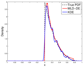
(a) Beta(1,4) distribution

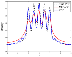
(b) Gaussian Mixture

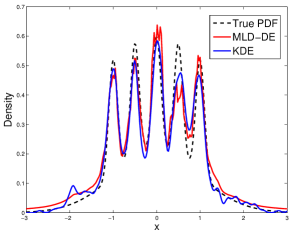
(c) Gaussian Mixture: optimal $\alpha$

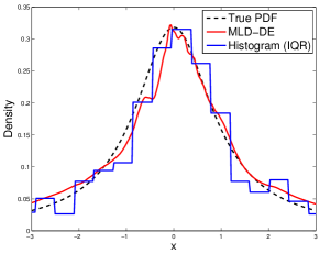
(d) Cauchy(0,1) distribution

Figure 3: Density estimates using MLD-DE, KDE and histogram approaches for the beta$(1,4)$, Gaussian mixture and Cauchy$(0,1)$ distributions.

For the MLD-DE and histogram-based estimators, estimates were obtained for 256 points in specified intervals. The interval used for each distribution is shown in the figures as the range over which the densities are plotted. Once the pointwise density estimates were calculated, interpolated density estimates were obtained using nearest-neighbor interpolation. For example, Figure 3 shows density estimates from a single sample using $\alpha=1/3$ for the beta (Figure 3(a)), Gaussian Mixture (Figure 3(b)) and Cauchy (Figure 3(d)), and with an optimal $\alpha$ for the Gaussian mixture (Figure 3(c)) obtained by simulation.

The sample size was again increased progressively starting with $N=125$ up to a maximum sample size $N=8000$. The MSE was calculated at every point of estimation, and then numerically integrated to obtain an estimate of the $L^{2}$-error. A total of 1000 trials were performed at each sample size to obtain the expected $L^{2}$-error for such sample size. Figure 4 shows the convergence plots obtained for the three densities using the various density estimation methods (the error bars are the size of the plotting symbols). We see that the performance of MLD-DE is comparable to that of the histogram method for the beta and Gaussian mixture densities, and KDE performs better with both these densities.

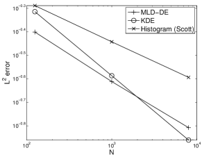
(a) Beta(1,4) distribution

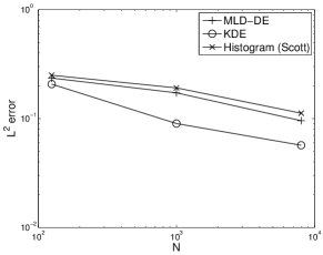
(b) Gaussian Mixture

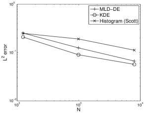
(c) Gaussian Mixture: optimal $\alpha$

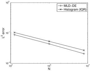
(d) Cauchy(0,1) density

Figure 4: $L^{2}$-convergence plots for various densities.

For the Cauchy density, both the histogram based on Scott’s rule and the KDE approach fail to converge. This is because Scott’s rule requires a finite second moment, whereas the kernel used in the KDE estimator is a Gaussian kernel, which has finite moments. But MLD-DE produces convergent estimates of the Cauchy density without any need to change the parameters from those used with the other densities. Furthermore, it also performs better than the IQR-based histogram, which is designed to be less sensitive to outliers in the data. Thus, MLD-DE provides a robust alternative to the histogram and kernel density estimation methods, while offering competitive convergence performance.

4.3 Spatial variation of the pointwise error

We now consider the pointwise bias and variance of MLD-DE. Given a fixed sample size, $N$, the bias and variance are estimated by simulations over 1000 trials. Figure 5 shows the results; it shows pointwise estimates of the mean and the standard error of the density estimates plotted alongside the true densities. We see that the pointwise variance increases with the value of the true density, while the bias is larger towards the corners of the estimation region. For comparison, Figure 6 shows analogous plots for the KDE and IQR histogram methods.

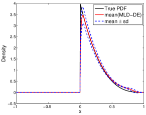
(a) Beta(1,4) distribution

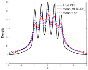
(b) Gaussian Mixture

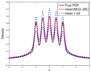
(c) Gaussian mixture: optimal $\alpha$

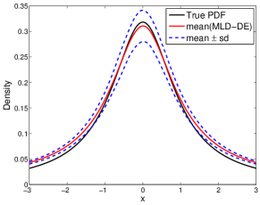
(d) Cauchy(0,1) distribution

Figure 5: Pointwise mean and variance of the MLD-DE estimates for various densities.

In particular, for the beta density (Figure 5(a)), the bias is smaller in the middle regions of the support of the density. However, the bias is large near the boundary point $x=0$, where the density has a discontinuity. Figure 5(b) shows the corresponding results for the Gaussian mixture. Again, we see a smaller variance in the tails of the density, but a larger bias in the tails. As the variance increases with the density, we see larger variances near the peaks than at the troughs. The results improve considerably with the optimal choice of $\alpha$ (Figure 5(c)), with a significant decrease in the bias. Figure 5(d) shows the results for the Cauchy density; these show a small bias in the tails but very low variance.

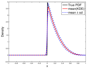
(a) Beta(1,4) distribution

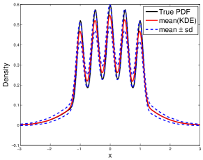
(b) Gaussian Mixture

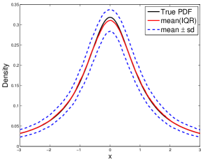
(c) Cauchy(0,1) distribution

Figure 6: Pointwise mean and variance of the adaptive KDE and IQR based histogram methods.

4.4 Effect of varying the tuning parameter $\alpha$

The MLD-DE method depends on the parameter, $\alpha$, that controls the ratio of number of subsets, $m_{N}$, to size, $s_{N}$, of each subset. This is similar to the dependence of histogram and KDE methods on a bandwidth parameter. However, MLD-DE allows the use of different $\alpha$ at each point of estimation without affecting the estimates at other points. This opens the possibility of flexible adaptive density estimation.

To evaluate the effect of $\alpha$ on the $L^{2}$-error, simulations were performed using values of $\alpha$ that increased from zero to one, with the total number of samples fixed to $N=1000$. The simulations were done for the beta$(1,4)$, Gaussian mixture and Cauchy$(0,1)$ distributions. Figure 7 shows plots of the estimated $L^{2}$-error as a function of $\alpha$ for the different densities.

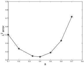
(a) Beta(1,4) distribution

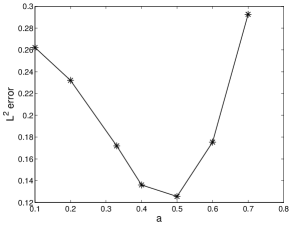
(b) Gaussian Mixture

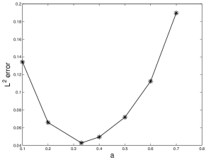
(c) Cauchy(0,1) distribution

Figure 7: $L^{2}$-error versus the parameter $\alpha$ for various densities. The sample size was fixed to $N=1000$. A large $\alpha$ implies a small number of subsets $m_{N}$, but a large number of samples $s_{N}$ in each subset, while a smaller $\alpha$ implies the converse.

All the curves have a similar profile, with the error increasing sharply for $\alpha\geq 0.7$; so the plots only show the errors for $\alpha\leq 0.8$. This indicates that, as we saw in Section 2, the number of subsets must be larger than their size. As we decrease $\alpha$ (i.e., increase the number of subsets), we see that the error is less sensitive to changes in the parameter. Decreasing $\alpha$ increases the bias, but keeps the variance low. In general, the ‘optimal’ value of $\alpha$ lies in between 0.2 and 0.6 for these simulations, which further restricts the search range of any optimization problem for $\alpha$.

An example of adaptive implementation

An adaptive approach was used to improve MLD-DE estimates of the Cauchy distribution. The numerical results in Figure 5(d) indicate that there is a larger bias in the tails of the distribution, while the theory indicates that the bias can be reduced by decreasing the number of subsets (correspondingly increasing the number of samples in each subset). The adaptive procedure used is as follows: (1) A pilot density was first computed using MLD-DE with $\alpha={1}/{3}$; (2) The points of estimation where the pilot density was within a fifth of the gap between the maximum and minimum density values from the minimum value (i.e., where the density was relatively small) were identified; (3) The MLD-DE procedure was repeated with the value $\alpha={1}/{2}$ for those points of estimation.

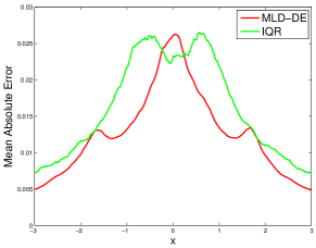
(a) Mean Absolute Error

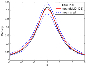
(b) Bias and Variance Error

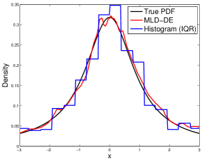
(c) Adaptive MLD Density

Figure 8: Cauchy density estimation with the adaptive MLD-DE

Figure 8 shows the results of this adaptive approach. We see that the bias has decreased significantly compared to that shown in the earlier plots for the non-adaptive approach. More sophisticated adaptive strategies can be employed with MLD-DE on account of its naturally adaptive nature, however a discussion of them is beyond the scope of this paper.

5 Discussion and generalizations

We have presented a simple, robust and easily parallelizable method for one-dimensional density estimation. Like nearest-neighbor density estimators, the method is based on nearest-neighbors but it offers the advantage of providing smoother density estimates, and has parallel complexity ${{\cal O}\left(N^{{1}/{3}}\right)}$ . Its tuning parameter is the number of subsets in which the original sample is divided. Theoretical results concerning the asymptotic distribution of the estimator were developed and its MSE was analyzed to determine a globally optimal split of the original sample into subsets. Numerical experiments illustrate that the method can recover different types of densities, including the Cauchy density, without the need for special kernels or bandwidth selections. Based on a heuristic analysis of high bias in low-density regions, an adaptive implementation that reduces the bias was also presented. Further work will be focused on more sophisticated adaptive schemes for one-dimensional density estimation and extensions to higher dimensions. We present here a brief overview of a higher dimensional extension of MLD-DE. Its generalization is straightforward but its convergence is usually not better than that of histogram methods. To see why, we consider the bivariate case. Let $(X,Y)$ be a random vector with PDF $f(x,y)$, and let $h(x,y)$ and $H(x,y)$ be the PDF and CDF of $(|X|,|Y|)$. It is easy to see that $h(0,0)=4f(0,0).$ In addition, let $q(t)=H(t,t)$, then $q^{\prime}(t)=\int_{0}^{t}h(t,y)\,dy+\int_{0}^{t}h(x,t)\,dx.$ It follows that (assuming continuity at $(0,0)$), $q^{\prime\prime}(0)=\lim_{t\to 0}q^{\prime}(t)/t=2\,h(0,0).$ Let ${\bf{X}}_{1}=(X_{1},Y_{1}),\ldots,{\bf{X}}_{N}=(X_{N},Y_{N})$ be iid vectors and define $U_{i}$ to be the product norm of ${\bf{X}}_{i}$: $U_{i}=\|{\bf{X}}_{i}\|_{\otimes}=\max\{\,|X_{i}|,\,|Y_{i}|\,\},$ and $Z=U_{(1)}$. Then

$$\mathbb{P}(\,Z>t\,) = \mathbb{P}(\,\|{\bf{X}}_{1}\|_{\otimes}>t,\ldots,\|{\bf{X}}_{N}\|_{\otimes}>t\,)=\mathbb{P}(\,\|{\bf{X}}_{1}\|_{\otimes}>t\,)^{N}$$

$$= [\,1-\mathbb{P}(\,\|{\bf{X}}_{1}\|_{\otimes}\leq t\,)\,]^{N}=[\,1-\mathbb{P}(\,|X_{1}|\leq t,|Y_{1}|\leq t\,)\,]^{N}$$

$$= [\,1-q(\,t\,)\,]^{N}.$$

Let $Q$ be the inverse of the function $q$. It is easy to check that $Q^{\prime}(z)=1/q^{\prime}(Q(z)).$ Proceeding as in the 1D case, we have

$$\mathbb{E}(\,Z^{2}\,) = 2\!\!\int_{0}^{\infty}t\,\mathbb{P}(\,Z>t\,)\,dt=2\!\!\int_{0}^{\infty}t\,[\,1-q(\,t\,)\,]^{N}\,dt=\int_{0}^{1}(Q^{2}(z))^{\prime}\,(1-z)^{N}\,dz.$$

Therefore $\mathbb{E}[\,(N+1)\,Z^{2}\,]=\int_{0}^{1}(Q^{2}(z))^{\prime}\,\delta_{N}(z)\,dz,$ and by the results in Section 2,

$$\lim_{n}\mathbb{E}[\,(N+1)\,Z^{2}\,]=(Q^{2}(z))^{\prime}|_{z=0}={1}/{h(0,0)}={1}/{(4\,f(0,0))}.$$

Furthermore,

$$\mathbb{E}[\,(N+1)\,Z^{2}\,]=\frac{1}{h(0,0)}+\frac{1}{N+2}\int_{0}^{1}(Q^{2}(z))^{\prime\prime}\,\delta_{N+1}(z)\,dz.$$

But, unlike in the 1D case, this time we have $\lim_{z\to 0}\,(Q^{2}(z))^{\prime\prime}={q^{(4)}(0)}/{(3q^{\prime\prime}(0))}\neq 0,$ and this makes the convergence rates closer to those of histogram methods.

Acknowledgments. We thank Y. Marzouk for reviewing our proofs, and D. Allaire, L. Ng, C. Lieberman and R. Stogner for helpful discussions. The first and third authors acknowledge the support of the the DOE Applied Mathematics Program, Awards DE-FG02-08ER2585 and DE-SC0009297, as part of the DiaMonD Multifaceted Mathematics Integrated Capability Center.

Appendix A Proofs

Proof of Lemma 1: (i) Since $f$ has right and left limits, $f(x_{*}^{+})$ and $f(x_{*}^{-})$, at $x_{*}$, we may re-define $f(x_{*})=(f(x_{*}^{+})+f(x_{*}^{-}))/2$. It then follows that

$$\lim_{y\to 0^{+}}g(y)=f(x_{*}^{+})+f(x_{*}^{-})=2f(x_{*})=g(0),$$

and therefore $g$ is right-continuous at zero. (ii) If $f$ has right and left derivatives, $f^{\prime}(x_{*}^{+})$ and $f^{\prime}(x_{*}^{-})$, at $x_{*}$, then $\lim_{y\to 0^{+}}({g(y)-g(0)})/{y}=f^{\prime}(x_{*}^{+})-f^{\prime}(x_{*}^{-})$ and therefore $g^{\prime}(0)$ exits, and $g^{\prime}(0)=0$ if $f$ is differentiable at $x_{*}$. ∎

The proof of Proposition 2.1 makes use of the elementary fact that the functions $\delta_{N}(z)=(N+1)(1-z)^{N}$, $z\in[0,1]$, define a sequence of Dirac functions. That is, for every $N\in\mathbb{N}$: (i) $\delta_{N}\geq 0$; (ii) $\int_{0}^{1}\delta_{N}(z)\,dz=1$; and (iii) for any $\varepsilon>0$ and $\delta\in(0,1)$, there is an integer $N_{0}$ such that $\int_{\delta}^{1}\delta_{N}(z)\,dz<\varepsilon$ for any $N\geq N_{0}$.

Proof of Lemma 2: The results follow from straightforward applications of the tail formula for the moments of a non-negative random variable. For (i) we have

$$\mathbb{E}{X_{(1),N}}=\int_{0}^{\infty}\mathbb{P}({X_{(1),N}}>t)\,dt=\int_{0}^{\infty}(1-G(t))^{N}\,dt.$$

Using the change of variable $z=G(t)$ leads to $\mathbb{E}{X_{(1),N}}=\int_{0}^{1}Q^{\prime}(z)\,(1-z)^{N}\,dz,$ and (1) follows. Version (2) follows from (1) using integration by parts, while version (2) follows using two integration by parts and the fact that $g^{\prime}(0)=0$. For (ii) we have something similar,

$$\mathbb{E}[{X_{(1),N}}^{2}] = \int_{0}^{\infty}2t\,\mathbb{P}({X_{(1),N}}>t)\,dt=\int_{0}^{\infty}2t\,(1-G(t))^{N}\,dt$$

$$= \int_{0}^{1}2\,Q(z)Q^{\prime}(z)\,(1-z)^{N}\,dz,$$

and therefore

$$(N+1)^{2}\,\mathbb{E}[{X_{(1),N}}^{2}] = (N+1)\int_{0}^{1}(Q^{2}(z))^{\prime}\,\delta_{N}(z)\,dz$$

$$= \left(\frac{N+1}{N+2}\right)\int_{0}^{1}(Q^{2}(z))^{\prime\prime}\,\delta_{N+1}(z)\,dz.$$

The last equation follows from integration by parts. $\square$

Proof of Proposition 2.1: Assume first that $H(0)\neq 0$. Let $\varepsilon>0$. By continuity at 0, there is $\eta\in(0,1)$ such that $|H(z)-H(0)|<\varepsilon/3$ if $0\leq z<\eta$. Also, by the properties of $\delta_{N}$ and, because $(N+1)/(N-m+1)\to 1$ as $N\to\infty$, there is an integer $N_{0}$ such that for $N>N_{0}$,

$$\int_{\eta}^{1}\!\!\delta_{N}(z)\,dz<\min\{{\varepsilon}/{(3|H(0)|)},{\varepsilon}/{(6C)}\}\,\,\mbox{and}\,\,(N+1)/(N-m+1)\leq 2.$$

Then,

$$\left|\int_{0}^{1}\!\!H(z)\,\delta_{N}(z)\,dz-H(0)\right| \leq \int_{0}^{\eta}|H(z)-H(0)|\,\delta_{N}(z)\,dz+\int_{\eta}^{1}|H(z)|\,\delta_{N}(z)\,dz$$

$$+\quad|H(0)|\int_{\eta}^{1}\delta_{N}(z)\,dz$$

$$\leq \varepsilon/3+\varepsilon/3+\int_{|z|\geq\eta}\!\!\!\!|H(z)|\,\delta_{N}(z)\,dz$$

$$\leq \varepsilon/3+\varepsilon/3+C\!\left(\frac{N+1}{N-m+1}\right)\!\!\int_{\eta}^{1}\delta_{N-m}(z)\,dz\leq\varepsilon$$

for $N>N_{0}+m$. The proof for $H(0)=0$ is analogous. $\square$

Proof of Proposition 2.2: (i) Since for a fixed $s_{N}$, $X^{(1)}_{(1),s_{N}},\ldots,X^{(m_{N})}_{(1),s_{N}}$ is an iid sequence, it follows from Corollary 1(i) that

$$\mathbb{E}\,\widehat{f^{-1}(0)}_{N}=({1}/{m_{N}})\sum_{k=1}^{m_{N}}\mathbb{E}[\,(s_{N}+1)X^{(k)}_{(1),s_{N}}\,]=\mathbb{E}[\,(s_{N}+1)X^{(1)}_{(1),s_{N}}\,]\to{1}/{g(0)}$$

as $N\to\infty$. For the second moment we have (for simplicity we define $a_{N}=s_{N}+1$),

$$\mathbb{E}[\,\widehat{f^{-1}(0)}_{N}^{2}\,] = \frac{1}{m_{N}^{2}}\sum_{k=1}^{m_{N}}\mathbb{E}[\,(a_{N}X^{(k)}_{(1),s_{N}})^{2}\,]+\frac{1}{m_{N}^{2}}\sum_{j\neq k}\mathbb{E}(\,a_{N}X^{(j)}_{(1),s_{N}}\,)\mathbb{E}(\,a_{N}X^{(k)}_{(1),s_{N}}\,)$$

$$= \frac{1}{m_{N}}\mathbb{E}[\,(a_{N}X^{(1)}_{(1),s_{N}})^{2}\,]+\left(\,\frac{m_{N}-1}{m_{N}}\,\right)[\,\mathbb{E}(\,a_{N}X^{(1)}_{(1),s_{N}}\,)\,]^{2}.$$

The variance and MSE are thus given by

$${\mathbb{V}{\rm ar}}[\,\widehat{f^{-1}(0)}_{N}^{2}\,] = ({1}/{m_{N}})\mathbb{E}[\,(a_{N}X^{(1)}_{(1),s_{N}})^{2}\,]-({1}/{m_{N}})[\,\mathbb{E}(\,a_{N}X^{(1)}_{(1),s_{N}}\,)\,]^{2}$$

$${\rm MSE}(\,\widehat{f^{-1}(0)}_{N}\,) = \frac{1}{m_{N}}\mathbb{E}[\,(a_{N}X^{(1)}_{(1),s_{N}})^{2}\,]+\left(\,\frac{m_{N}-1}{m_{N}}\,\right)[\,\mathbb{E}(\,a_{N}X^{(1)}_{(1),s_{N}}\,)\,]^{2}$$

$$-\frac{2}{g(0)}\mathbb{E}(\,a_{N}X^{(1)}_{(1),s_{N}}\,)+\frac{1}{g(0)^{2}}.$$

By (6) and (9), the MSE converges to zero as $N\to\infty$, Hence, (13) follows.
(ii) Since limit (14) implies (15) by Cramer’s $\delta$-method, it is sufficient to prove (14). Define $\mu_{N}=\mathbb{E}X_{(1),s_{N}}^{(k)}$,  $Z_{k,s_{N}}=\,X_{(1),s_{N}}^{(k)}-\mu_{N}$, and $Y_{k,N}=a_{N}\,Z_{k,s_{N}}/\sqrt{m_{N}}$ for $k\leq m_{N}$, with $Y_{k,N}=0$, otherwise. The variables $Y_{1,N},\ldots,Y_{N,N}$ are independent, zero-mean and, by Corollary 1(iii),

$$\sum_{k=1}^{N}\mathbb{E}(\,Y_{k,N}^{2}\,)={\mathbb{V}{\rm ar}}(\,a_{N}X_{(1),s_{N}}^{(1)}\,)\to 1/g(0)^{2},$$ (17)

as $N\to\infty$. Fix $\varepsilon>0$. We show that the following Lindeberg condition is satisfied:

$$\sum_{k=1}^{N}\mathbb{E}(\,Y_{k,N}^{2}\,I_{Y_{k,N}^{2}>\varepsilon^{2}}\,)=\mathbb{E}(\,a_{N}^{2}Z_{1,N}^{2}\,I_{a_{N}^{2}Z_{1,N}^{2}>\varepsilon^{2}{m_{N}}}\,)\to 0.$$ (18)

To see this, note that since $X_{i}\geq 0$, we have $a_{N}^{2}Z_{1,s_{N}}^{2}\leq a_{N}^{2}X_{(1),s_{N}}^{2}+a_{N}^{2}\mu_{N}^{2}.$ Since $a_{N}\mu_{N}$ has a finite limit, the difference $\varepsilon m_{N}-a_{N}^{2}\mu_{N}^{2}$ is positive for $N$ larger than some integer $N_{1}$. For simplicity, define $c_{N}^{2}=\varepsilon^{2}m_{N}-a_{N}^{2}\mu_{N}^{2}$. We then have

$$\mathbb{E}(\,a_{N}^{2}Z_{1,N}^{2}\,I_{a_{N}^{2}Z_{1,N}^{2}>\varepsilon^{2}m_{N}}\,)\leq\mathbb{E}(\,a_{N}^{2}X_{(1),s_{N}}^{2}I_{a_{N}^{2}X_{(1),s_{N}}^{2}>c_{N}^{2}}\,)+a_{N}^{2}\mu_{N}^{2}\mathbb{P}(a_{N}^{2}X_{(1),s_{N}}^{2}>c_{N}^{2}).$$

Since $m_{N}/s_{N}\to\infty$, it follows that $c_{N}/a_{N}\to\infty$ and therefore $\mathbb{P}(\,X>c_{N}/a_{N}\,)<1/2$ for $N$ larger than an integer $N_{2}$. Hence, for $N>\max\{N_{1},N_{2}\}$,

$$a_{N}^{2}\mu_{N}^{2}\mathbb{P}(a_{N}^{2}X_{(1),s_{N}}^{2}>c_{N}^{2})\!\!\! = \!\!a_{N}^{2}\mu_{N}^{2}\mathbb{P}(\,X>c_{N}/a_{N}\,)^{s_{N}}\leq a_{N}^{2}\mu_{N}^{2}/2^{s_{N}}$$

$$\mathbb{E}(\,a_{N}^{2}X_{(1),s_{N}}^{2}I_{a_{N}^{2}X_{(1),s_{N}}^{2}>c_{N}^{2}}\,)\!\!\! = 2\!\!\int_{0}^{\infty}t\,\mathbb{P}(a_{N}^{2}X_{(1),s_{N}}^{2}I_{a_{N}^{2}X_{(1),s_{N}}^{2}>c_{N}^{2}}>t)\,dt$$

$$\leq 2\!\!\int_{0}^{\infty}t\,\mathbb{P}(\,a_{N}X_{(1),s_{N}}>t,a_{N}X_{(1),s_{N}}>c_{N}\,)\,dt$$

$$= 2\mathbb{P}(\,X_{(1),s_{N}}>c_{N}/a_{N}\,)\!\int_{0}^{c_{N}}t\,dt+2\!\!\int_{c_{N}}^{\infty}t\,\mathbb{P}(\,X_{(1),s_{N}}>t/a_{N}\,)\,dt.$$

The tail condition (with $C>0$ and integer $k>0$) on the last integral yields

$$\mathbb{E}(\,a_{N}^{2}X_{(1),s_{N}}^{2}I_{a_{N}^{2}X_{(1),s_{N}}^{2}>c_{N}^{2}}\,) \leq c_{N}^{2}\mathbb{P}(\,X_{(1),s_{N}}>c_{N}/a_{N}\,)+Ca_{N}^{2}\!\!\int_{G(c_{N}/a_{N})}^{1}(1-z)^{s_{N}-k}\,dz$$

$$= c_{N}^{2}\mathbb{P}(\,X>c_{N}/a_{N}\,)^{s_{N}}+\frac{Ca_{N}^{2}}{a_{N}+k}\mathbb{P}(\,X>c_{N}/a_{N}\,)^{a_{N}-k}$$

$$\leq \frac{c_{N}^{2}}{2^{s_{N}}}+\frac{C\,a_{N}^{2}}{(a_{N}+k)\,2^{a_{N}-k}}.$$

Since the right hand-side converges to zero, (18) follows. By Lindeberg-Feller’s theorem, (17) and (18) imply that

$$\sqrt{m_{N}}\,[\,\widehat{f^{-1}(0)}_{N}-\mathbb{E}\widehat{f^{-1}(0)}_{N}\,]\stackrel{{\scriptstyle{\cal L}}}{{\longrightarrow}}N(0,1/g(0)^{2}).$$ (19)

On the other hand, by (8),

$$\sqrt{m_{N}}\,[\,a_{N}\mu_{N}-1/g(0)\,]\to 0$$ (20)

because $\sqrt{m_{N}}/s_{N}^{2}\to 0$. Combining (8) and (20) yields (14). Note that since $s_{N}^{2}>\sqrt{m_{N}}$, it follows that the ME of $\widehat{f^{-1}(0)}_{N}$ is ${{\cal O}\left(1/m_{N}\right)}$, and using a simple Taylor expansion one also finds that the MSE of $\widehat{f(0)}_{N}$ is also ${{\cal O}\left(1/m_{N}\right)}$. $\square$

References

- [Botev et al., 2010] Botev, Z. I., Grotowski, J. F., and Kroese, D. P. (2010). Kernel density estimation via diffusion. The Annals of Statistics, 38(5):2916–2957.
- [Buch-Larsen et al., 2005] Buch-Larsen, T., Nielsen, J. P., Guillén, M., and Bolancé, C. (2005). Kernel density estimation for heavy-tailed distributions using the Champernowne transformation. Statistics, 39(6):503–516.
- [DasGupta, 2008] DasGupta, A. (2008). Asymptotic Theory of Statistics and Probability. Springer.
- [Efromovich, 2010] Efromovich, S. (2010). Orthogonal series density estimation. WIREs Comp. Stat., 2:467–476.
- [Freedman and Diaconis, 1981] Freedman, D. and Diaconis, P. (1981). On the histogram as a density estimator: theory. Probability Theory and Related Fields, 57(4):453–476.
- [Fukunaga and Hostetler, 1973] Fukunaga, K. and Hostetler, L. (1973). Optimization of nearest-neighbor density estimates. Information Theory, IEEE Transactions on, 19(3):320–326.
- [Hall et al., 2008] Hall, P., Park, B. U., and Samworth, R. J. (2008). Choice of neighbor order in nearest-neighbor classification. The Annals of Statistics, 36(5):2135–2152.
- [Kung et al., 2012] Kung, Y. H., Lin, P. S., and Kao, C. H. (2012). An optimal k-nearest neighbor for density estimation. Statistics & Probability Letters, (82):1786–1791.
- [Li, 1984] Li, K.-C. (1984). Consistency for cross-validated nearest-neighbor estimates in nonparametric regression. The Annals of Statistics, pages 230–240.
- [Parzen, 1962] Parzen, E. (1962). On estimation of a probability density function and mode. The Annals of Mathematical Statistics, 33(3):1065–1076.
- [Raykar et al., 2010] Raykar, V. C., Duraiswami, R., and Zhao, L. H. (2010). Fast computation of kernel estimators. Journal of Computational and Graphical Statistics, 19(1):205–220.
- [Scott, 1979] Scott, D. W. (1979). On optimal and data-based histograms. Biometrika, 66(3):605–610.
- [Scott, 1992] Scott, D. W. (1992). Multivariate Density Estimation. Theory, Practice and Visualization. Wiley.
- [Silverman, 1986] Silverman, B. W. (1986). Density Estimation for Statistics and Data Analysis. Chapman & Hall/CRC.
- [Wand and Jones, 1995] Wand, M. P. and Jones, M. C. (1995). Kernel Smoothing. Chapman & Hall.
- [Wasserman, 2006] Wasserman, L. (2006). All of Nonparametric Statistics. Springer.