An integrable deformation of an ellipse of small eccentricity is an ellipse

Abstract.

The classical Birkhoff conjecture claims that the boundary of a strictly convex integrable billiard table is necessarily an ellipse (or a circle as a special case). In the paper we show that a version of this conjecture is true for tables bounded by small perturbations of ellipses of small eccentricity.

1. Introduction

Let $\Omega\subset\mathbb{R}^{2}$ be a strictly convex domain; we say that $\Omega$ is $C^{r}$ if its boundary is a $C^{r}$-smooth curve. We consider the billiard problem inside $\Omega$, which is then commonly called the “billiard table”. The problem was first investigated by Birkhoff (see [3]) and is described as follows: a massless billiard ball moves with unit speed and no friction following a rectilinear path inside the domain $\Omega$. When the ball hits the boundary, it is reflected elastically according to the law of optical reflection: the angle of reflection equals the angle of incidence. Such trajectories are called broken geodesics, as they correspond to local minimizers of the distance functional.

We call a (possibly not connected) curve $\widehat{\Gamma}\subset\Omega$ a caustic if any billiard orbit having one segment tangent to $\widehat{\Gamma}$ has all its segments tangent to $\widehat{\Gamma}$.

We call a billiard $\Omega$ locally integrable if the union of all caustics has nonempty interior; likewise, a billiard $\Omega$ is said to be integrable (see [10]) if the union of all smooth convex caustics, denoted $\mathcal{C}_{\Omega}$, has nonempty interior.

It follows by rather elementary geometrical considerations, (but see e.g. [20, Theorem 4.4] for a detailed proof) that a billiard in an ellipse is integrable: its caustics are indeed co-focal ellipses and hyperbolas. A long standing open question asks whether or not there exist integrable billiards which are different from ellipses.

Birkhoff Conjecture (see [16], [10]).

If the billiard in $\Omega$ is integrable, then $\partial\Omega$ is an ellipse.

The most notable result related to the Birkhoff Conjecture is due to Bialy (see [2] but also [24]) who proved that, if convex caustics completely foliate $\Omega$, then $\Omega$ is necessarily a disk. On the other hand, it is simple to construct smooth (but not analytic) locally integrable billiards different from ellipses. In fact, it suffices to perturb an ellipse away from a neighborhood of the two endpoints of the minor axis. More interestingly, Treschev (see [22]) gives indication that there are analytic locally integrable billiards such that the dynamics around one elliptic point is conjugate to a rigid rotation.

There is a remarkable relation between properties of the billiard dynamics in $\Omega$ and the spectrum of the Laplace operator in $\Omega$. Given a smooth domain $\Omega$, the length spectrum of $\Omega$ is defined as the collection of perimeters of its periodic trajectories, counted with multiplicity:

$$\mathcal{L}_{\Omega}:=\mathbb{N}\{\text{lengths of periodic trajectories in }\Omega\}\cup\mathbb{N}\ell_{\partial\Omega},$$

where $\ell_{\partial\Omega}$ denotes the length of $\partial\Omega$.

Let $\text{Spec}\,\Delta$ denote the spectrum of the Laplace operator in $\Omega$ with (e.g) Dirichlet boundary condition, i.e. the set of $\lambda$ so that

$$\Delta u =\lambda u, u =0\text{ on }\partial\Omega.$$

Andersson–Melrose (see [1, Theorem (0.5)], which substantially generalizes some earlier result by [5, 6]) proved that, for strictly convex $C^{\infty}$ domains, the following relation between the wave trace and the length spectrum holds:

$$\textup{sing\ supp}\left(t\mapsto\sum_{\lambda_{j}\in\text{Spec}\,\Delta}\exp(i\sqrt{-\lambda_{j}}t)\right)\subset\pm\mathcal{L}_{\Omega}\cup\{0\}.$$

Generically (i.e. when each element of the length spectrum has multiplicity one and the corresponding periodic orbits satisfy a non-degeneracy condition) the above inclusion becomes an equality and the Laplace spectrum determines the length spectrum (see e.g. [15] and references therein).

This is, of course, related to inverse spectral theory and to the famous question by M. Kac [12]: “Can one hear the shape of a drum?”, which more formally translates to “Does the Laplace spectrum determine a domain?” There is a number of counterexamples to this question (see e.g. [8, 19, 23]), but the domains considered in such examples are neither smooth nor convex.

In [18], P. Sarnak conjectures that the set of smooth convex domains isospectral to a given smooth convex domain is finite. Hezari–Zelditch, going in the affirmative direction, proved in [11] that, given an ellipse $\mathcal{E}$, any one-parameter $C^{\infty}$-deformation $\Omega_{\varepsilon}$ which preserves the Laplace spectrum (with respect to either Dirichlet or Neumann boundary conditions) and the $\mathbb{Z}_{2}\times\mathbb{Z}_{2}$ symmetry group of the ellipse has to be flat (i.e., all derivatives have to vanish for $\varepsilon=0$). Further historical remarks on the inverse spectral problem can also be found in [11].

2. Our main result

Given a strictly convex domain $\Omega$, we define the associated billiard map $f_{\Omega}$ as follows. Let us fix a point $P_{0}\in\partial\Omega$ and denote with $s$ the arc-length parametrization of $\partial\Omega$ starting at $P_{0}$ in the counter-clockwise direction; let $P_{s}$ denote the point on $\partial\Omega$ parametrized by $s$. We define the billiard map

(1) $$f_{\Omega}:\mathbb{T}_{\Omega}\times[0,\pi] \to\mathbb{T}_{\Omega}\times[0,\pi],$$

$$(s,\varphi) \mapsto(s^{\prime},\varphi^{\prime}),$$

where $\mathbb{T}_{\Omega}=\mathbb{R}/\ell_{\partial\Omega}\mathbb{Z}$, $\ell_{\partial\Omega}$ is the length of $\partial\Omega$, $P_{s^{\prime}}$ is the reflection point of a ray leaving $P_{s}$ with angle $\varphi$ with respect to the counter-clockwise tangent ray to the boundary $\partial\Omega$ and $\varphi^{\prime}$ is the angle of incidence of the ray at $P_{s^{\prime}}$ with the clockwise tangent. If there is no confusion we will drop the subscript $\Omega$ and simply refer to the billiard map as $f$ and let $\mathbb{T}=\mathbb{T}_{\Omega}$.

In the remaining part of this paper, we agree that all caustics that we will consider will be smooth and convex; we will refer to such curves simply as caustics.

Let $\widehat{\Gamma}$ be a caustic for $\Omega$; for any $s\in\mathbb{T}_{\Omega}$ there exist two rays leaving $P_{s}$ which are tangent to $\widehat{\Gamma}$, one aligned with the counter-clockwise tangent of $\widehat{\Gamma}$ and the other one with the clockwise tangent; let us denote with $\varphi^{\pm}_{\widehat{\Gamma}}(s)$ their corresponding angles of reflection. Observe that, by reversibility of the dynamics, the trajectory associated with $\varphi^{-}$ is the time-reversal of the trajectory associated with $\varphi^{+}$, i.e. $\varphi^{-}=\pi-\varphi^{+}$. We can, thus, restrict our analysis to (e.g.) $\varphi^{+}$; in doing so we will drop, for simplicity, the superscript $+$ from our notations.

The graph $\Gamma=\{(s,\varphi_{\widehat{\Gamma}}(s))\}_{s\in\mathbb{T}}$   is, by definition of a caustic, a (non-contractible) $f$-invariant curve. Therefore, the restriction $f|_{\Gamma}$ is a homeomorphism of the circle, and, as such, it admits a rotation number, which we denote with $\omega$. In fact (since we have chosen $\varphi^{+}$ over $\varphi^{-}$), we always have $0<\omega\leq 1/2$.

Definition.

We say $\widehat{\Gamma}$ is an integrable rational caustic if the corresponding (non-contractible) invariant curve $\Gamma$ consists of periodic points; in particular, the corresponding rotation number is rational. If $\Omega$ admits integrable rational caustics of rotation number $1/q$ for all $q>2$, we say that $\Omega$ is rationally integrable.

Remark.

A more standard definition of integrability requires existence of a “nice” first integral. Existence of a “nice” first integral for a billiard does not imply integrability of any caustic of rational rotation number. For instance, the invariant curve corresponding to points belonging to the coinciding separatrix arcs of a hyperbolic periodic orbit of $f$ is not integrable.

The following lemma provides a sufficient (although a priori weaker) condition for rational integrability.

Lemma 1.

Assume the interior of the union of all smooth convex caustics $\textup{int}\,{}\mathcal{C}_{\Omega}$ of a billiard $\Omega$ contains caustics of rotation number $1/q$ for any $q\geq 2$, then $\Omega$ is rationally integrable.

Proof.

It is known that if a caustic with rational rotation number belongs to the interior of a foliation with caustics, then it is integrable (see e.g. [20, Corollary 4.5] for the general statement and [9, Proposition 2.8] for the special case of an ellipse). Thus, our assumption guarantees the rational integrability of $\Omega$. ∎

Let us denote with $\mathcal{E}_{e}\subset\mathbb{R}^{2}$ an ellipse of eccentricity $e$ and perimeter $1$.

Main Theorem.

There exists $e_{0}>0$ and $\varepsilon_{0}>0$ such that for any $0\leq e\leq e_{0}$, $0\leq\varepsilon<\varepsilon_{0}$, any rationally integrable $C^{39}$-smooth domain $\Omega$ so that $\partial\Omega$ is $C^{{39}}$-$\varepsilon$-close to $\mathcal{E}_{e}$ is an ellipse.

Remark.

We will indeed prove a slightly stronger version of the above theorem, stated as Theorem 25.

Remark.

Our requirements for smoothness are probably not optimal, but they are crucial for the approach used in our proof (see the proof of Lemma 24 and, in particular, Footnote 9). One could possibly relax them using [4].

Acknowledgments: We thank L. Bunimovich, D. Jakobson, I. Polterovich, A. Sorrentino, D. Treschev, J. Xia, S. Zelditch and the anonymous referee for their most useful comments which allowed to vastly improve the exposition of our result. JDS acknowledges partial NSERC support. VK acknowledges partial support of the NSF grant DMS-1402164.

3. Our strategy and the outline of the paper

Let us start by exploring the simplified setting of integrable infinitesimal deformations of a circle; we then use this insight to describe the main strategy of our proof in the general case. Let $\Omega_{0}$ be the unit disk and let us denote polar coordinates on the plane with $(r,\phi)$. Let $\Omega_{\varepsilon}$ be a one-parameter family of deformations given in polar coordinates by $\partial\Omega_{\varepsilon}=\{(r,\phi)=(1+\varepsilon n(\phi)+O(\varepsilon^{2}),\phi)\}$. Consider the Fourier expansion of $n$:

$$n(\phi)=n_{0}+\sum_{k>0}n^{\prime}_{k}\sin(k\phi)+n^{\prime\prime}_{k}\cos(k\phi).$$

Theorem (Ramirez-Ros [17]).

If $\Omega_{\varepsilon}$ has an integrable rational caustic $\Gamma_{1/q}$ of rotation number $1/q$ for all sufficiently small $\varepsilon$, then $n^{\prime}_{kq}=n_{kq}^{\prime\prime}=0$ for any $k\in\mathbb{N}$.

Let us now assume that the domains $\Omega_{\varepsilon}$ are rationally integrable for all sufficiently small $\varepsilon$: then the above theorem implies that $n^{\prime}_{k}=n^{\prime\prime}_{k}=0$ for $k>2$, i.e.

$$n(\phi) =n_{0}+n^{\prime}_{1}\cos\phi+n_{1}^{\prime\prime}\sin\phi+n^{\prime}_{2}\cos 2\phi+n_{2}^{\prime\prime}\sin 2\phi$$

$$=n_{0}+n_{1}^{*}\cos(\phi-\phi_{1})+n_{2}^{*}\cos 2(\phi-\phi_{2})$$

where $\phi_{1}$ and $\phi_{2}$ are appropriately chosen phases.

Remark 2.

Observe that

• $n_{0}$ corresponds to an homothety;

• $n_{1}^{*}$ corresponds to a translation in the direction forming an angle $\phi_{1}$ with the polar axis ($\{\phi=0\}$);

• $n_{2}^{*}$ corresponds to a deformation into an ellipse of small eccentricity with the major axis meeting the polar axis at the angle $\phi_{2}$.

This implies that, infinitesimally (as $\varepsilon\to 0$), rationally integrable deformations of a circle are tangent to the $5$-parameter family of ellipses.

Observe that in principle, in the above theorem, one may need to take $\varepsilon\to 0$ as $q\to\infty$. On the other hand, we are studying a situation in which $\varepsilon>0$ is small but not infinitesimal; hence we cannot use directly the above theorem to prove our result, and we need to pursue a more elaborate strategy, which we now describe.

Let $\Omega_{0}$ be a strictly convex domain (to fix ideas the reader may assume $\Omega_{0}$ to be an ellipse) and consider a tubular neighborhood $U_{\Omega_{0}}$ of $\partial\Omega_{0}$ so that for any $P\in U_{\Omega_{0}}$ we can associate the tubular coordinates $(s,n)$, where $s$ is the $s$-coordinate of the orthogonal projection of $P$ onto the boundary $\partial\Omega_{0}$ and ${n}$ is the oriented distance of $P$ along the orthogonal direction to $\partial\Omega_{0}$ defined so that $n>0$ outside (resp. $n<0$ inside) of $\Omega_{0}$.

We can, thus, identify any given domain $\Omega$ so that $\partial\Omega\subset U_{\Omega_{0}}$ with the graph of a function ${\bf n}(s)$ in tubular coordinates. In order to do that one can project points from $\partial\Omega$ to $\partial\Omega_{0}$ and lift points from $\partial\Omega_{0}$ to $\partial\Omega$. In the sequel we will only consider perturbations $\Omega$ which can be described by a function ${\bf n}(s)$ of this form and we introduce the following (slightly abusing, but suggestive) notation

$$\partial\Omega=\partial\Omega_{0}+{\bf n}.$$

Our strategy now proceeds as follows: let $\Omega_{0}$ be an ellipse $\mathcal{E}_{e}$ of eccentricity $e$ and perimeter $1$; in particular, all rational caustics of rotation number $1/q$ for $q>2$ are integrable.

Step 1: We derive a quantitative necessary condition for preservation of an integrable rational caustic (see Theorem 3 in Section 4).

Step 2: We define Deformed Fourier modes for the case of ellipses; they will be denoted by $\{c_{0},c_{q},s_{q}:q>0\}$ and satisfy the following properties:

• (relation with Fourier Modes) There exists (see Lemma 20) $C^{*}(e)>0$ with $C^{*}(e)\to 0$ as $e\to 0$ so that $\|c_{0}-1\|_{C^{0}}\leq C^{*}(e)$ and for any $q\geq 1$

  $$\|c_{q}-\cos(2\pi q\cdot)\|_{C^{0}} \leq C^{*}(e)/q, \|s_{q}-\sin(2\pi q\cdot)\|_{C^{0}} \leq C^{*}(e)/q.$$

• (transformations preserving integrability) We define (in Section 6) the functions

  $$c_{0},\,c_{1},\,s_{1},\,c_{2},\,s_{2}$$

  having the same meaning described in the previous remark: they generate homotheties, translations and hyperbolic rotations about an arbitrary axis.

• (annihilation of inner products) Let ${\bf n}$ identify a $C^{r}$ deformation of $\Omega_{0}$ and consider, for $\varepsilon\in(-\varepsilon_{0},\varepsilon_{0})$, the one-parameter family of domains

  $$\partial\Omega_{\varepsilon}:=\partial\Omega_{0}+\varepsilon{\bf n}.$$

  For any $q>2$, we define (in Section 5) functions $c_{q},s_{q}$ so that if $\Omega_{\varepsilon}$ has an integrable rational caustic $\widehat{\Gamma}^{\varepsilon}_{1/q}$ of rotation number $1/q$ for all sufficiently small $\varepsilon$, then

  (2) $$\langle{\bf n},c_{q}\rangle=\langle{\bf n},s_{q}\rangle=0,$$

  where $\langle\cdot,\cdot\rangle$ is a weighted $L^{2}$ inner product. In fact, in Lemma 13 we derive a perturbative version of the above infinitesimal orthogonality conditions. More precisely: if, for some sufficiently $C^{1}$-small, $C^{5}$-perturbation ${\bf n}$, the domain bounded by $\partial\Omega=\partial\Omega_{0}+{\bf n}$ has an integrable rational caustic $\widehat{\Gamma}_{1/q}$, then we can replace (2) with

  (3) $$\langle{\bf n},c_{q}\rangle =O(q^{8}\|{\bf n}\|_{C^{1}}^{2}), \langle{\bf n},s_{q}\rangle =O(q^{8}\|{\bf n}\|_{C^{1}}^{2}).$$

  Observe that, as we hinted at earlier, the above estimate is necessarily non-uniform in $q$. Notice that the functions $c_{q},s_{q}$ can be explicitly defined using elliptic integrals via action-angle coordinates (see (22)).

• (linear independence) For sufficiently small eccentricity (see Section 7), the functions $\{c_{0},c_{q},s_{q}\,:\,q>0\}$ form a (non-orthogonal) basis of $L^{2}$.

Step 3: We then conclude the proof (in Section 8) using the following approximation result (Lemma 24): if $\Omega_{\varepsilon}$ is rationally integrable and $\partial\Omega_{\varepsilon}$ is an $O(\varepsilon)$-perturbation of an ellipse $\partial\Omega_{0}=\mathcal{E}_{e}$ of small eccentricity $e$, then there exists an ellipse $\bar{\mathcal{E}}$ such that $\partial\Omega_{\varepsilon}$ is an $O(\varepsilon^{\beta})$-perturbation of $\bar{\mathcal{E}}$ for some $\beta>1$. This step is done as follows

• For a fixed $\varepsilon=\|{\bf n}\|_{C^{1}}$ and each $2<q\leq q_{0}(\varepsilon)=[\varepsilon^{-1/9}]$, condition (3) implies that the size of the $q$-th generalized Fourier coefficients is small and, therefore, their sum up to $q_{0}$ is bounded by $\varepsilon^{\beta}$.

• Due to decay of the generalized Fourier coefficients we can also show that the sum over $q>q_{0}$ is bounded by $\varepsilon^{\beta}$.

Combining the above estimates, we gather that $\partial\Omega_{\varepsilon}$ can be approximated by an ellipse $\bar{\mathcal{E}}$ with an error $O(\varepsilon^{\beta})$, where $\bar{\mathcal{E}}$ is the ellipse generated by projecting ${\bf n}$ onto the subspace generated by the first $5$ Deformed Fourier modes. Applying this result to the best approximation of $\partial\Omega_{\varepsilon}$ by an ellipse, we obtain a contradiction unless $\partial\Omega_{\varepsilon}$ is itself an ellipse.

Remark.

We emphasize that our condition on eccentricity is not an abstract smallness assumption. More specifically: one has to check that some explicit condition on the eccentricity (given in (28)) holds true.

4. A sufficient condition for rational integrability, the Deformation Function, and action-angle variables

Let $\Omega_{0}=\mathcal{E}_{e}\subset\mathbb{R}^{2}$ be an ellipse of eccentricity $e$ and perimeter $1$; let $f=f_{\mathcal{E}_{e}}$ be the associated billiard map. For convenience, let us fix $P_{0}$ be one of the end-points of the major axis. For $0<\omega<1/2$, let $\hat{\Gamma}_{\omega}$ be the caustic of rotation number $\omega$ and $\Gamma_{\omega}$ be the corresponding invariant curve of $f$. Then, for any $\omega$, there exists a parametrization $\theta$ of $\mathcal{E}_{e}$ so that $f$ acts as a rigid rotation of angle $\omega$, i.e. if $S(\theta;\omega)$ denotes the change of variables from the $\theta$-parametrization to the arc-length parametrization, for any $\theta\in\mathbb{T}$ we have:

(4) $$f(S(\theta;\omega),\Phi(\theta;\omega))=(S(\theta+\omega;\omega),\Phi(\theta+\omega;\omega)),$$

where we introduced the shorthand notation $\Phi(\theta;\omega)=\varphi_{\widehat{\Gamma}_{\omega}}(S(\theta;\omega))$. In other words, $(S,\Phi)$ is the change of variables from the action-angle coordinates $(\theta,\omega)$ to arc-length and reflection angle. Geometrically: given $S(\theta;\omega)$, consider the trajectory leaving $P_{S(\theta;\omega)}$ with angle $\Phi(\theta;\omega)$; this ray will be tangent to $\widehat{\Gamma}_{\omega}$ and land at the point parametrized by $S(\theta+\omega;\omega)$ with angle $\Phi(\theta+\omega;\omega)$ with respect to the tangent to $\mathcal{E}_{e}$ at $S(\theta+\omega;\omega)$.

We normalize $S$ so that $S(0;\omega)=0$ for all $\omega\in(0,1/2)$. Following Tabanov (see [21]) we can assume $S$ and $\Phi$ to be analytic in both $\theta$ and $\omega$. In particular, for each $\omega\in(0,1/2)$ the map $S(\cdot;\omega)$ is an (analytic) circle diffeomorphism. Observe additionally that both functions depend analytically on the parameter $e$ and, moreover, for $e=0$ we have $S(\theta;\omega)=\theta$ and $\Phi(\theta;\omega)=\pi\omega$.

Let now $\Omega$ be a deformation of $\mathcal{E}_{e}$ identified by a $C^{{39}}$ function ${\bf n}$. Given $p/q\in\mathbb{Q}\cap(0,1/2)$ with $p$ and $q$ relatively prime, let us define the Deformation Function:

(5) $$\mathcal{D}\left({\bf n},S,\Phi,\frac{p}{q}\right)(\theta)=2\sum_{k=1}^{q}{\bf n}\left(S\left(\theta+k\frac{p}{q};\frac{p}{q}\right)\right)\sin\Phi\left(\theta+k\frac{p}{q};\frac{p}{q}\right).$$

In Theorem 3 below we show that the Deformation Function is the leading term of the change of perimeter of the possibly non-convex polygon inscribed in $\mathcal{E}_{e}$ corresponding to an orbit of rotation number $p/q$ starting at $P_{S(\theta)}$. In order state more precisely the above consideration, we now proceed to introduce some further notation.

First, since in the present article we are interested only in caustics of rotation number $1/q$, we restrict the analysis to this case. Let us thus introduce the convenient shorthand notations $S_{q}=S(\cdot,1/q)$ and $\Phi_{q}=\Phi(\cdot,1/q)$. Recall that for any ellipse $\mathcal{E}_{e}$, every caustic $\widehat{\Gamma}_{1/q}$ of rotation number $1/q$ with $q>2$ is an integrable rational caustic. Recall also that, for any $0\leq s<1$, $P_{s}$ denotes the point whose arc-length distance from $P_{0}$ in the counter-clockwise direction equals $s$. Define

$$P^{0}_{k}(\theta) =P_{S_{q}(\theta+k/q)} \text{for }k =0,\cdots,q-1.$$

In other words, for any $\theta\in\mathbb{T}$ we associate the corresponding $q$-periodic orbit tangent to the caustic $\widehat{\Gamma}_{1/q}$ given by the points $P^{0}_{0}(\theta),\cdots,P^{0}_{q-1}(\theta)$. The variational characterization of periodic orbits (see e.g. [3]) implies that periodic orbits are given by the vertices of an inscribed convex $q$-gon with one vertex at $P_{S_{q}(\theta)}$ and whose perimeter is a stationary value. Let $L^{0}_{q}(\theta)$ be the perimeter of this $q$-gon, i.e.

$$L^{0}_{q}(\theta)=\sum_{k=0}^{q-1}\|P^{0}_{k+1}(\theta)-P^{0}_{k}(\theta)\|,$$

where $\|\cdot\|$ is the Euclidean distance. Then, since $\widehat{\Gamma}_{1/q}$ is an integrable rational caustic, we conclude that $L^{0}_{q}(\theta)$ is actually constant in $\theta$. In fact, all periodic orbits belonging to a smooth one-parameter family have the same, constant, perimeter.

Let us denote with $P^{\prime}_{0}(\theta)\in\partial\Omega$ the lift of $P^{0}_{0}(\theta)\in\partial\Omega_{0}$ to $\partial\Omega$. Since $\Omega$ is strictly convex, for each $\theta\in\mathbb{T}$, there is a convex $q$-gon starting at $P^{\prime}_{0}(\theta)$ of maximal perimeter. Denote its vertices by $P^{\prime}_{k}(\theta),\ k=0,\cdots,q-1$ and its perimeter by

$$L^{\prime}_{q}(\theta)=\sum_{k=0}^{q-1}\|P^{\prime}_{k+1}(\theta)-P^{\prime}_{k}(\theta)\|.$$

If, moreover, $\Omega$ admits an integrable rational caustic of rotation number $1/q$, then the points $P^{\prime}_{0}(\theta),\cdots,P^{\prime}_{q-1}(\theta)$ are actually the reflection points of the $q$-periodic orbit of rotation number $1/q$ starting at $P^{\prime}_{0}(\theta)$. By the arguments given above, $L^{\prime}_{q}(\theta)$ is also constant.

Theorem 3.

Let $\Omega_{0}=\mathcal{E}_{e}$ be an ellipse of eccentricity $0\leq e<1$ and perimeter $1$, and let $(S,\Phi)$ be the corresponding functions defined above. Then there is $c=c(e)>0$ such that for any integer $q$, $q>2$ and $C^{5}$ deformation $\partial\Omega:=\mathcal{E}_{e}+{\bf n}$ so that $\Omega$ admits an integrable rational caustic $\Gamma_{1/q}$ of rotation number $1/q$ and $\ q^{8}\|{\bf n}\|_{C^{1}}<c$:

$$\max_{\theta}\left|L_{q}^{\prime}(\theta)-L_{q}^{0}(\theta)-\mathcal{D}({\bf n},S,\Phi;1/q)(\theta)\right|\leq C\,q^{8}\|{\bf n}\|_{C^{1}}^{2},$$

where $C=C(e,\|{\bf n}\|_{C^{5}})$ depends on the eccentricity $e$ and monotonically on the $C^{5}$-norm of ${\bf n}$, but is independent of $q$.

Remark.

Notice that in [14, Proposition 11] a different (weaker, but cleaner) version of this statement is given, where it suffices to know only $S(\theta,\omega)$. We also point out that $c(e)\to 0$ as $e\to 1$.

Proof of Theorem 3.

Let $\alpha_{k}(\theta)$ be the angle between $P^{\prime}_{k}(\theta)-P^{0}_{k}(\theta)$ and the positive tangent to $\mathcal{E}_{e}$ at $P^{0}_{k}(\theta)$ (see Figure 1). We assume $\alpha_{k}(\theta)$ to be positive towards the exterior of $\mathcal{E}_{e}$, i.e. if $P^{\prime}_{k}(\theta)$ is outside of $\mathcal{E}_{e}$, then $\alpha_{k}(\theta)\in(0,\pi)$. Introduce the displacements

$$v_{k}(\theta)=\|P^{\prime}_{k}(\theta)-P^{0}_{k}(\theta)\|$$

and let $\varphi_{k}(\theta)=\Phi_{q}(\theta+k/q)$. By definition of action-angle coordinates, the edge $P^{0}_{k+1}(\theta)-P^{0}_{k}(\theta)$ has reflection angle $\varphi_{k}(\theta)$ at $P^{0}_{k}(\theta)$ and $\varphi_{k+1}(\theta)$ at $P^{0}_{k+1}(\theta)$ respectively. Finally, let us introduce the notation $l^{0}_{k}(\theta)=\|P^{0}_{k+1}(\theta)-P^{0}_{k}(\theta)\|$ and $l^{\prime}_{k}(\theta)=\|P^{\prime}_{k+1}(\theta)-P^{\prime}_{k}(\theta)\|$. Observe that by Corollary 10, for each $k=0,\cdots,q-1$ we have

(6) $$\frac{1}{\Xi q}\leq l^{\prime}_{k}(\theta)\leq\frac{\Xi}{q}\ \text{ for some }\ \Xi=\Xi(e,\|{\bf n}\|_{C^{5}})>1,$$

and $\Xi$ depends monotonically on $\|{\bf n}\|_{C^{5}}$. For $k=0,\cdots,q-1$, project $P^{\prime}_{k}(\theta)$ onto $\mathcal{E}_{e}$ by the orthogonal projection and denote the projected point by $\bar{P}^{\prime}_{k}(\theta)$. Observe that, by construction, $\bar{P}^{\prime}_{0}(\theta)=P^{0}_{0}(\theta)$. Denote, moreover, with $\bar{\varphi}^{+}_{k}$ (resp. $\bar{\varphi}^{-}_{k}$) the angle between $\bar{P}^{\prime}_{k+1}(\theta)-\bar{P}^{\prime}_{k}(\theta)$ (resp. $\bar{P}^{\prime}_{k}(\theta)-\bar{P}^{\prime}_{k-1}(\theta)$) and the positive (resp. negative) tangent to $\mathcal{E}_{e}$ at $\bar{P}^{\prime}_{k}(\theta)$ (see Figure 2).

Lemma 4.

Let $\Xi$ be the constant appearing in (6); for any $k=0,\cdots,q-1$:

$$|\bar{\varphi}_{k}^{+}-\bar{\varphi}_{k}^{-}|\leq 5\Xi\,q\,\|{\bf n}\|_{C^{1}}.$$

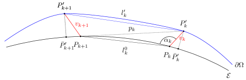
Figure 1. Two orbits: unperturbed (in black) and perturbed (in blue)

Proof.

Since $\|P^{\prime}_{k}-\bar{P}^{\prime}_{k}\|\leq\|{\bf n}\|_{C^{0}}$ for any $k=0,\cdots,q-1$, the angle between the $k$-th perturbed edge and the $k$-th projected edge satisfies

$$\sphericalangle\{P^{\prime}_{k}(\theta)-P^{\prime}_{k+1}(\theta),\bar{P}^{\prime}_{k}(\theta)-\bar{P}^{\prime}_{k+1}(\theta)\}\leq\frac{2\|{\bf n}\|_{C^{0}}}{l^{\prime}_{k}(\theta)-2\|{\bf n}\|_{C^{0}}}\leq{4\Xi\,q\,\|{\bf n}\|_{C^{0}}}$$

where in the last inequality we have used (6): in fact, we know $l^{\prime}_{k}(\theta)>\Xi/q$ and by our assumptions on ${\bf n}$ we have $\|{\bf n}\|_{C^{0}}\leq\|{\bf n}\|_{C^{1}}<c/q^{8}$, thus, if $c<1/\Xi$, since $q>2$:

$$l^{\prime}_{k}(\theta)-2\|{\bf n}\|_{C^{0}}\geq l^{\prime}_{k}(\theta)/2>1/(2\Xi q).$$

Since $\Omega$ has an integrable rational caustic $\Gamma_{1/q}$ of rotation number $1/q$, the collection $P^{\prime}_{k}(\theta),\ k=0,\cdots,q-1$ corresponds to a $q$-periodic orbit, thus, the angle of incidence at $P^{\prime}_{k}(\theta)$ of $P^{\prime}_{k}(\theta)-P^{\prime}_{k+1}(\theta)$ equals the angle of reflection of $P^{\prime}_{k-1}(\theta)-P^{\prime}_{k}(\theta)$. See Figure 2: the angle between the tangent to $\partial\Omega$ at $P^{\prime}_{k}(\theta)$ and the tangent to $\mathcal{E}_{e}$ at the projected point $\bar{P}^{\prime}_{k}(\theta)$ is bounded above by ${\bf n}^{\prime}(S_{q}(\theta+k/q))$, hence by $\|{\bf n}\|_{C^{1}}$. Therefore, adding the two deviations coming from the discrepancy of the tangents to $\partial\Omega$ (resp. $\mathcal{E}_{e}$) and the discrepancy of end-points $P^{\prime}_{i}(\theta)$ (resp. $\bar{P}^{\prime}_{i}(\theta)$) with $i=k\pm 1,k$ we get that

$$|\bar{\varphi}^{+}_{k}-\bar{\varphi}^{-}_{k}|\leq 4\Xi\,q\,\|{\bf n}\|_{C^{0}}+2\|{\bf n}\|_{C^{1}},$$

from which we conclude our proof. ∎

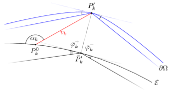
Figure 2. Reflection angles: in blue (above) the trajectory of the periodic orbit given by $P^{\prime}_{0},\cdots,P^{\prime}_{q-1}$; in black (below) the pseudo-orbit given by $\bar{P}^{\prime}_{0},\cdots,\bar{P}^{\prime}_{q-1}$.

Lemma 5.

For each $k=0,\cdots,q-1$ let $\bar{\theta}_{k}$ be so that $\bar{P}^{\prime}_{k}(\theta)=P_{S_{q}(\bar{\theta}_{k})}$. Then there exists $C=C(e,\|{\bf n}\|_{C^{5}})$ so that, in the above notations, for any  $k=0,\cdots,q-1$:

(7) $$|\bar{\theta}_{k}-\theta_{k}| \leq Cq^{3}\|{\bf n}\|_{C^{1}}, v_{k}(\theta) \leq Cq^{3}\|{\bf n}\|_{C^{1}}.$$

Proof.

The basic idea of the proof is to consider the worst case scenario for the deviation of the reflection angles $\bar{\varphi}^{\pm}_{k}(\theta)$ from $\varphi_{k}(\theta)$. Since, unless $\mathcal{E}_{e}$ is a circle, the reflection angles $\varphi_{k}$ vary depending on the reflection point, it is more convenient to keep track of a first integral, which is constant along any orbit on the ellipse $\mathcal{E}_{e}$ and, therefore, cannot change too rapidly for the perturbed domain $\Omega$. We now quantitatively explain this phenomenon. Recall that for the ellipse one can explicitly define a conserved quantity (a first integral), as follows. For simplicity, assume $\mathcal{E}_{e}$ is centered at the origin and that the major axis is horizontal; let

$$\mathcal{E}_{e}=\{x^{2}+y^{2}/(1-e^{2})=a_{e}^{2}\},$$

where $a_{e}$ is the semi-major axis, given by $a_{e}=1/(4E(e))$, and $E(e)$ is the complete elliptic integral of the second kind, so that the ellipse $\mathcal{E}_{e}$ has, as we always assume, perimeter $1$. Let us then introduce the so-called elliptical coordinates $(\mu,\psi)$ on $\mathbb{R}^{2}$ as follows:

$$x =h\cdot\cosh\mu\cdot\cos\psi, y =h\cdot\sinh\mu\cdot\sin\psi$$

where $h^{2}=a_{e}^{2}e^{2},\ 0\leq\mu<\infty,\ 0\leq\psi<2\pi$. The family of co-focal ellipses $\mu=$const and hyperbolas $\psi=$const form an orthogonal net of curves. The ellipse $\mathcal{E}_{e}$ has the equation $\mu=\mu_{0}$, where $\cosh^{2}\mu_{0}=e^{-2}>1$. Thus, the length parametrization $s$ of the ellipse can be given as a function of $\psi$, (see e.g. [21] for an explicit formula): Then, the billiard map has a first integral given by

$$I(\psi,\varphi)=\cos^{2}\varphi+\frac{\cos^{2}\psi}{\cosh^{2}\mu_{0}}\sin^{2}\varphi;$$

observe that $I(\psi,\varphi)=I(\psi,\pi-\varphi)$. Recall that $\theta$ denotes the action-angle parametrization of $\mathcal{E}_{e}$ in action-angle coordinates with rotation number $1/q$ and $S_{q}$ is the change of variables to arc-length coordinates. Since the elliptic angle $\psi$ is an analytic function of the arc-length parametrization $s$ and $S$, in turn, is an analytic function of $\theta$ (see (4)), we can define the first integral $I(\theta,\varphi)$ in the $(\theta,\varphi)$ coordinates. Notice that $\cosh^{2}\mu_{0}>1\geq\cos^{2}\psi$; hence

$$\partial_{\varphi}I(\psi,\varphi)=\left(\frac{\cos^{2}\psi}{\cosh^{2}\mu_{0}}-1\right)\,\sin 2\varphi;$$

observe that for any $\psi$, the function $I(\psi,\cdot)$ is strictly decreasing on $(0,\pi/2)$; moreover $|\partial_{\varphi}I|<1$ and

(8) $$|\partial_{\varphi}I|\in[1-\cosh^{-2}\mu_{0},2]\,\varphi\ \text{ for $\varphi\in[0,\pi/6]$}.$$

Moreover, this holds in both $(\psi,\varphi)$ and $(\theta,\varphi)$ coordinates.

Then we claim that there exists ${k_{*}}$ so that $\bar{\varphi}_{{k_{*}}}^{-}\leq\Phi_{q}(\bar{\theta}_{k_{*}})\leq\bar{\varphi}_{{k_{*}}}^{+}$. Observe that by definition

$$f(S_{q}(\bar{\theta}_{k}),\bar{\varphi}_{k}^{+})=(S_{q}(\bar{\theta}_{k+1}),\bar{\varphi}_{k+1}^{-});$$

by well-known properties of monotone twist maps, no orbit can cross the invariant curve $\Gamma_{1/q}$, thus we obtain that if $\bar{\varphi}^{+}_{k}<\Phi_{q}(\bar{\theta}_{k})$ (resp. $\bar{\varphi}^{+}_{k}>\Phi_{q}(\bar{\theta}_{k})$), then $\bar{\varphi}^{-}_{k+1}<\Phi_{q}(\bar{\theta}_{k+1})$ (resp. $\bar{\varphi}^{-}_{k+1}>\Phi_{q}(\bar{\theta}_{k+1})$). We conclude that if our claim does not hold, necessarily, either $\bar{\varphi}_{k}^{+}<\Phi_{q}(\bar{\theta}_{k})$ or $\bar{\varphi}_{k}^{+}>\Phi_{q}(\bar{\theta}_{k})$ for all $k=0,\cdots,q-1$. In the first case, the twist condition implies that $\bar{\theta}_{k+1}-\bar{\theta}_{k}<1/q$; but this is a contradiction, since $\bar{\theta}_{q}=\bar{\theta}_{0}+1$ (passing to the covering space $\mathbb{R}$). Similar arguments in the second case also lead to a contradiction; this, in turn, implies our claim. Moreover, Lemma 4 implies that

$$\bar{\varphi}^{+}_{{k_{*}}}-\Phi_{q}(\bar{\theta}_{k_{*}})\leq 5\Xi\,q\,\|{\bf n}\|_{C^{1}}<5q^{-7}.$$

Define now the instant first integral $I_{k}^{\pm}=I(\bar{\theta}_{k},\bar{\varphi}_{k}^{\pm})$; then $I^{+}_{k}=I^{-}_{k+1}$ and since

$$|I^{+}_{k}-I^{-}_{k}|\leq\left|\int_{\bar{\varphi}_{k}^{-}}^{\bar{\varphi}_{k}^{+}}\partial_{\varphi}I(\bar{\theta}_{k},\varphi)d\varphi\right|$$

and $\Phi_{q}(\bar{\theta}_{k_{*}})<C(e)/q$ (applying Corollary 9 to $\mathcal{E}_{e}$), Lemma 4 and (8) allow us to conclude (possibly choosing a larger $C$) that

(9) $$|I^{+}_{k_{*}}-I_{*}|<C\,\|{\bf n}\|_{C^{1}},$$

where $I_{*}=I(\theta,\varphi_{0}(\theta))$ and $C=C(e,\|{\bf n}\|_{C^{5}})$. Inducing at most $q$ times and applying repeatedly the same argument we conclude that $|I_{0}^{\pm}-I_{*}|<Cq\|{\bf n}\|_{C^{1}}$. This in turn implies that

$$|\bar{\varphi}_{0}^{\pm}(\theta)-\varphi_{0}(\theta)|<Cq^{2}\|{\bf n}\|_{C^{1}}$$

and inducing on $k$ and using again Lemma 4 we conclude (possibly choosing a larger $C$)

$$|\bar{\theta}_{k}-\theta_{k}| <Cq^{3}\|{\bf n}\|_{C^{1}}.$$

The second bound of (7) follows immediately by applying the triangle inequality. ∎

Lemma 6.

In the notations introduced above we have

(10) $$\Big{|}l^{\prime}_{k}(\theta)-l^{0}_{k}(\theta) -v_{k}(\theta)\cos\left(\varphi_{k}(\theta)+\alpha_{k}(\theta)\right)$$

$$+v_{k+1}(\theta)\cos\left(\varphi_{k+1}(\theta)-\alpha_{k+1}(\theta)\right)\Big{|}\leq 10\frac{v_{k}(\theta)^{2}+v_{k+1}(\theta)^{2}}{l^{0}_{k}(\theta)}.$$

Proof.

Let $p_{k}(\theta)=\|P^{\prime}_{k}(\theta)-P^{0}_{k+1}(\theta)\|$; applying the Cosine Theorem to the triangle $\bigtriangleup P^{0}_{k}(\theta)P^{0}_{k+1}(\theta)P^{\prime}_{k}(\theta)$ we have

$$p_{k}(\theta)^{2} =v_{k}(\theta)^{2}+l^{0}_{k}(\theta)^{2}-2v_{k}(\theta)l^{0}_{k}(\theta)\cos(\varphi_{k}(\theta)+\alpha_{k}(\theta)).$$

Likewise, applying it to the triangle $\bigtriangleup P^{0}_{k+1}(\theta)P^{\prime}_{k+1}(\theta)P^{\prime}_{k}(\theta)$ we have

$$l^{\prime}_{k}(\theta)^{2}=v_{k+1}(\theta)^{2}+p_{k}(\theta)^{2}+2v_{k+1}(\theta)p_{k}(\theta)\cos(\varphi_{k+1}(\theta)-\alpha_{k+1}(\theta)-\delta_{k+1}(\theta)),$$

where $\delta_{k+1}(\theta)$ is the oriented angle $\sphericalangle(P^{0}_{k}(\theta)P^{0}_{k+1}(\theta)P^{\prime}_{k}(\theta))$. Combining the above expressions we get

(11) $$l^{\prime}_{k}(\theta)^{2}-l^{0}_{k}(\theta)^{2} =v_{k}(\theta)^{2}+v_{k+1}(\theta)^{2}-2v_{k}(\theta)l^{0}_{k}(\theta)\cos(\varphi_{k}(\theta)+\alpha_{k}(\theta))$$

$$\phantom{=}+2v_{k+1}(\theta)p_{k}(\theta)\cos(\varphi_{k+1}(\theta)-\alpha_{k+1}(\theta)-\delta_{k+1}(\theta)).$$

Observe that by the triangle inequality:

$$l^{0}_{k}(\theta)-v_{k}(\theta)-v_{k+1}(\theta)\leq l^{\prime}_{k}(\theta),p_{k}(\theta)\leq l^{0}_{k}(\theta)+v_{k}(\theta)+v_{k+1}(\theta).$$

Moreover, elementary geometry implies $|\sin\delta_{k+1}(\theta)|\leq v_{k}(\theta)/l^{0}_{k}(\theta)$. Now (10) immediately follows dividing both sides of (11) by $l^{\prime}_{k}(\theta)+l^{0}_{k}(\theta)$ and using the above estimates. ∎

We can now conclude the proof of Theorem 3; observe that by definition $L^{0}_{q}(\theta)=\sum_{k=0}^{q-1}l^{0}_{k}(\theta)$ and likewise $L^{\prime}_{q}(\theta)=\sum_{k=0}^{q-1}l^{\prime}_{k}(\theta)$. By Lemma 6 we thus gather:

$$\Big{|}L^{\prime}_{q}(\theta)-L^{0}_{q}(\theta) -\sum_{k=0}^{q-1}v_{k}(\theta)\cos\left(\varphi_{k}(\theta)+\alpha_{k}(\theta)\right)$$

$$+\sum_{k=0}^{q-1}v_{k+1}(\theta)\cos\left(\varphi_{k+1}(\theta)-\alpha_{k+1}(\theta)\right)\Big{|}\leq 20\sum_{k=0}^{q-1}\frac{v_{k}(\theta)^{2}}{l^{0}_{k}(\theta)}.$$

Observe that

$$\sum_{k=0}^{q-1}\Big{[} -v_{k}(\theta)(\cos\varphi_{k}(\theta)\cos\alpha_{k}(\theta)-\sin\varphi_{k}(\theta)\sin\alpha_{k}(\theta))$$

$$+v_{k+1}(\theta)(\cos\varphi_{k+1}(\theta)\cos\alpha_{k+1}(\theta)+\sin\varphi_{k+1}(\theta)\sin\alpha_{k+1}(\theta))\Big{]}$$

$$=2\sum_{k=0}^{q-1}v_{k}(\theta)\sin\varphi_{k}(\theta)\sin\alpha_{k}(\theta).$$

Notice that, by (7), we have $v_{k}(\theta)\sin\alpha_{k}(\theta)={\bf n}(S_{q}(\theta+k/q))+O(q^{6}\|{\bf n}\|^{2}_{C^{1}})$. Therefore,

$$\left|L^{\prime}_{q}(\theta)-L^{0}_{q}(\theta)-\sum_{k=0}^{q-1}{\bf n}(S_{q}(\theta+k/q))\sin\Phi_{q}(\theta+k/q)\right|\leq Cq^{8}\|{\bf n}\|_{C^{1}}^{2}.$$

This completes the proof of Theorem 3. ∎

5. Lazutkin parametrization and Deformed Fourier Modes

It turns out that for nearly glancing orbits, i.e. orbits having small reflection angle, it is more convenient to study the billiard map $f$, which has been defined in (1), in Lazutkin coordinates (see [13]), which we now proceed to define.

Let $\Omega$ be a strictly convex domain; recall that $s$ denotes the arc-length parametrization of $\partial\Omega$ and denote with $\rho(s)$ its radius of curvature at $s$. Observe that if $\Omega$ is $C^{r}$, then $\rho$ is $C^{r-2}$. Define the Lazutkin parametrization of the boundary:

(12) $$x(s) =C_{\Omega}\,\int_{0}^{s}\,\rho(\sigma)^{-2/3}\ d\sigma, \text{ where }C_{\Omega} =\left[\int_{0}^{\ell_{\partial\Omega}}\rho(\sigma)^{-2/3}d\sigma\right]^{-1}.$$

We call the Lazutkin map the following change of variables:

(13) $$\Psi_{\text{L}} :(s,\varphi)\mapsto(\,x=x(s),y(s,\varphi)=4C_{\Omega}\,\rho(s)^{1/3}\sin(\varphi/2)\,).$$

Also let us introduce the Lazutkin density

(14) $$\mu(x)=\frac{1}{2C_{\Omega}\rho(x)^{1/3}},$$

where we denote by $\rho(x)=\rho(s(x))$ the radius of curvature in the Lazutkin parametri- zation, where $s(x)$ can be obtained by inverting (12). Observe that $\mu(x)=\pi$ for a circle and varies analytically with the eccentricity for ellipses.

By replacing the arc-length parametrization $s$ with the Lazutkin parametrization $x$ in the definition of the tubular coordinates, we obtain the definition of the Lazutkin tubular coordinates. With a slight abuse of notation, we denote the corresponding perturbation function with ${\bf n}(x)$. Observe that if $\partial\Omega=\mathcal{E}_{e}$ is an ellipse, $\rho$ is analytic and, thus, the Lazutkin parametrization is itself an analytic parametrization of $\mathcal{E}_{e}$.

Lemma 7.

Let $\Omega$ be a perturbation of the ellipse $\mathcal{E}_{e}$ identified by the function ${\bf n}$ (i.e. $\partial\Omega=\mathcal{E}_{e}+{\bf n}$). Consider another ellipse $\bar{\mathcal{E}}$ sufficiently close to $\mathcal{E}_{e}$: let ${\bf n}_{\bar{\mathcal{E}}}$ so that $\bar{\mathcal{E}}=\mathcal{E}_{e}+{\bf n}_{\bar{\mathcal{E}}}$ and $(\bar{x},\bar{n})$ denote Lazutkin tubular coordinates in a neighborhood of $\bar{\mathcal{E}}$. If $\bar{\mathcal{E}}$ is sufficiently close to $\mathcal{E}_{e}$ we can write $\partial\Omega=\bar{\mathcal{E}}+\bar{\bf n}$ for some function $\bar{\bf n}(\bar{x})$. There exists $C=C(e)$ so that

(15) $$|\bar{\bf n}(x)-({\bf n}(x)-{\bf n}_{\bar{\mathcal{E}}}(x))|\leq C\|{\bf n}_{\bar{\mathcal{E}}}\|_{C^{1}}\|{\bf n}-{\bf n}_{\bar{\mathcal{E}}}\|_{C^{1}}.$$

In particular, for any $C^{\prime}>1$, if $\bar{\mathcal{E}}$ is sufficiently close to $\mathcal{E}_{e}$ we have

(16) $$\frac{1}{C^{\prime}}\|{\bf n}-{\bf n}_{\bar{\mathcal{E}}}\|_{C^{1}}\leq\|\bar{\bf n}\|_{C^{1}}\leq C^{\prime}\|{\bf n}-{\bf n}_{\bar{\mathcal{E}}}\|_{C^{1}}.$$

Proof.

Consider the change of variables $(x,n)\mapsto(\bar{x},\bar{n})$ defined in the intersection of the tubular neighborhoods of $\mathcal{E}_{e}$ and $\bar{\mathcal{E}}$. Clearly this is an analytic change of variables, that is $C\|{\bf n}_{\bar{\mathcal{E}}}\|_{C^{0}}$-close to the identity in any $C^{r}$-norm for some $C$ depending on $r$ and on the eccentricity $e$. In particular, we have:

$$\bar{x}(x,n) =x+\varrho_{1}(x,n),$$

$$\bar{n}(x,n) =(n-{\bf n}_{\bar{\mathcal{E}}}(x))(1+\varrho_{2}(x,n)),$$

where $\varrho_{1}$ and $\varrho_{2}$ are analytic functions that are $C\|{\bf n}_{\bar{\mathcal{E}}}\|_{C^{0}}$-small in any $C^{r}$-norm for some $C$ depending on $r$ and on the eccentricity $e$. Observe that if $x_{\text{c}}$ is a critical point of ${\bf n}_{\bar{\mathcal{E}}}$, we have by construction $\bar{n}(x_{\text{c}},n)=n-{\bf n}_{\bar{\mathcal{E}}}(x_{\text{c}})$. Since $\partial\Omega=\mathcal{E}_{e}+{\bf n}=\bar{\mathcal{E}}+\bar{\bf n}$, we conclude that

$$\bar{n}(x,{\bf n}(x))=\bar{\bf n}(\bar{x}(x,{\bf n}(x))).$$

Let us denote with $\bar{x}_{\Omega}(x)=\bar{x}(x,{\bf n}(x))$; observe that by our previous estimates we have that $\bar{x}_{\Omega}$ is a diffeomorphism and $\bar{x}_{\Omega}^{\prime}=1+O(\|{\bf n}_{\bar{\mathcal{E}}}\|_{C^{1}}\|{\bf n}\|_{C^{1}})$. By the implicit function theorem we conclude that

$$\bar{\bf n}^{\prime}(\bar{x}_{\Omega}(x)))=\frac{\partial_{x}\bar{n}(x,{\bf n}(x))+\partial_{n}\bar{n}(x,{{\bf n}}(x)){\bf n}^{\prime}(x)}{\partial_{x}\bar{x}(x,{{\bf n}}(x))+\partial_{n}\bar{x}(x,{{\bf n}}(x)){\bf n}^{\prime}(x)}.$$

Using the above expression for $n(\bar{x},\bar{n})$ and $x(\bar{x},\bar{n})$ we gather

$$\bar{\bf n}^{\prime}(\bar{x}_{\Omega}(x)))=\frac{({\bf n}^{\prime}(x)-{\bf n}^{\prime}_{\bar{\mathcal{E}}}(x))(1+O(\|{\bf n}_{\bar{\mathcal{E}}}\|_{C^{0}}))}{1+O(\|{\bf n}_{\bar{\mathcal{E}}}\|_{C^{0}})}.$$

Thus, integrating:

$$\bar{\bf n}(\bar{x}) =\bar{\bf n}(x_{\text{c}})+\int_{x_{\text{c}}}^{\bar{x}}\bar{\bf n}^{\prime}(\bar{x})d\bar{x}$$

$$=\left[{\bf n}(x_{\Omega}^{-1}(\bar{x}))-{\bf n}_{\bar{\mathcal{E}}}(x_{\Omega}^{-1}(\bar{x}))\right](1+O(\|{\bf n}_{\bar{\mathcal{E}}}\|_{C^{0}}))$$

$$={\bf n}(\bar{x})-{\bf n}_{\bar{\mathcal{E}}}(\bar{x})+O(\|{\bf n}_{\bar{\mathcal{E}}}\|_{C^{1}}\|{\bf n}-{\bf n}_{\bar{\mathcal{E}}}\|_{C^{1}}),$$

that is (15). It is then immediate to obtain (16). ∎

Consider now the billiard map in Lazutkin coordinates $f_{\text{L}}=\Psi_{\text{L}}\circ f\circ\Psi_{\text{L}}^{-1}$; then $f_{\text{L}}$ has the following form (see e.g. [13, (1.4)]):

(17) $$f_{\text{L}}:(x,y) \to(x+y+y^{3}g(x,y),y+y^{4}h(x,y)),$$

where $g$ and $h$ can be expressed analytically in terms of derivatives of the curvature radius $\rho$ up to order $3$: hence, if $\Omega$ is $C^{r}$, $g,h$ are $C^{r-5}$. Recall that $\widehat{\Gamma}_{1/q}\subset\Omega$ denotes a caustic of rotation number $1/q$, while $\Gamma_{1/q}$ denotes the associated non-contractible invariant curve for the billiard map $f$. We denote by $\Gamma_{\text{L},1/q}$ the corresponding invariant curve for the billiard map $f_{\text{L}}$ in Lazutkin coordinates, i.e. $\Gamma_{\text{L},1/q}=\Psi_{\text{L}}\,\Gamma_{1/q}$. Moreover, let us introduce the change of variables from action-angle coordinates $(\theta,\omega)$ to Lazutkin coordinates, i.e $(X(\theta,\omega),Y(\theta,\omega))=\Psi_{\text{L}}(S(\theta,\omega),\Phi(\theta,\omega))$; as before, we define $X_{q}(\theta)=X(\theta,1/q)$ and $Y_{q}(\theta)=Y(\theta,1/q)$.

Lemma 8.

Let $\Omega$ be a $C^{5}$ strictly convex domain; for $k\in\mathbb{Z}$, let $(x_{k},y_{k})=f_{\text{L}}^{k}(x_{0},y_{0})$ be a periodic orbit of rotation number $1/q$ with $q>2$. Then there exists $C$ depending on $\|\rho\|_{C^{3}}$ and independent of $q$, such that for $0\leq k<q$

(18) $$\left|y_{k}-\frac{1}{q}\right| <\frac{C}{q^{3}}, \left|\tilde{x}_{k}-\tilde{x}_{0}-\frac{k}{q}\right| <\frac{C}{q^{2}},$$

where $\tilde{x}_{k}$ is a lift of $x_{k}$ to $\mathbb{R}$.

Corollary 9.

Let $\Omega$ be a $C^{5}$ strictly convex domain and let $\Gamma_{\text{L},1/q}$ be the invariant curve corresponding to an integrable rational caustic of rotation number $1/q$ with $q>2$, given by

$$\Gamma_{\text{L},1/q}=\{(x,y_{q}(x)):\ x\in\mathbb{T}\}.$$

Then there exists $C$ depending on $\|\rho\|_{C^{3}}$, such that

(19) $$\left|y_{q}(x)-\frac{1}{q}\right| <\frac{C}{q^{3}} \ x\in\mathbb{T}$$ for any .

Moreover, in the case $\partial\Omega$ is an ellipse $\mathcal{E}_{e}$ of eccentricity $e$ and perimeter $1$, the constant $C$ can be chosen to depend continuously on $e$ and satisfies $C(e)\to 0$ as $e\to 0$.

Proof.

The proof of the first part immediately follows from the first bound of (18). Observe now that if $\partial\Omega$ is an ellipse of eccentricity $e$, $\Gamma_{\text{L},1/q}=\{(X_{q}(\theta),Y_{q}(\theta))\}_{\theta\in\mathbb{T}}$ where both $X_{q}$ and $Y_{q}$ vary analytically with $e$. Moreover, if $\partial\Omega$ is a circle, $Y_{q}(\theta)$ is the constant function equal to $1/q$. We conclude that we can choose $C(e)$ so that it is continuous in $e$ and $\lim_{e\to 0}C(e)=0$. ∎

Corollary 10.

Let $\Omega$ be a $C^{5}$ strictly convex domain and $q>2$. Let $(s_{k},\varphi_{k}),\ k=0,\cdots,q-1$ be a $q$-periodic orbit of rotation number $1/q$ and $P_{k},\ k=0,\cdots,q-1$ be the corresponding collision points on $\partial\Omega$. Then there is $\Xi=\Xi(\Omega)>1$, depending on $\|\rho\|_{C^{3}}$, such that the Euclidean length of each edge $\|P_{k+1}-P_{k}\|$ satisfies

$$\frac{1}{\Xi q}\leq\|P_{k+1}-P_{k}\|\leq\frac{\Xi}{q}.$$

Moreover, if $\Omega$ is a perturbation ${\bf n}$ of an ellipse $\mathcal{E}_{e}$ (i.e. $\partial\Omega=\mathcal{E}_{e}+{\bf n}$), then $\Xi$ can be chosen to depend continuously on the eccentricity $e$ and $\|{\bf n}\|_{C^{5}}$.

Proof.

Recall that, by definition, $y(s,\varphi)=4\,C_{\Omega}\,\rho^{1/3}(s)\sin(\varphi/2)$. By Lemma 8 we have $y\in[1/q-C/q^{3},1/q+C/q^{3}]$ for some $C$ depending on $\rho$ only. Therefore, $\sin(\varphi/2)\in[1/Cq-1/q^{3},C/q+C^{2}/q^{3}]$. Since the angle of reflection is of order $1/q$ and curvature is uniformly bounded, we get the required bound on the distance $\|P_{k+1}-P_{k}\|$. ∎

Proof of Lemma 8.

Choose $q_{0}$ (sufficiently large depending on $\|\rho\|_{C^{3}}$) to be specified in due course and assume $q\geq q_{0}$. Observe that we can choose $C$ so large that our statement trivially holds for any $2<q<q_{0}$. First of all, we claim that we have the preliminary bound

$$y_{k} \leq\frac{C_{1}}{q}, \text{ for }0\leq k<q,$$

where $C_{1}$ is a large constant depending on the curvature $\rho$. In fact, let $(s_{k},\varphi_{k})=\Psi_{\text{L}}^{-1}(x_{k},y_{k})$, so that

$$(s_{k+1},\varphi_{k+1})=f(s_{k},\varphi_{k})$$

and let $\tilde{s}_{k}$ be a lift to $\mathbb{R}$. Since $\tilde{s}_{q}=\tilde{s}_{0}+1$, there exists $0\leq{k_{*}}<q$ so that $0<\tilde{s}_{{k_{*}}+1}-\tilde{s}_{k_{*}}\leq 1/q$. For fixed $s_{k}$, we can find a function $\varphi(s_{k+1})$ so that the ray leaving $s_{k}$ with angle $\varphi(s_{k+1})$ will collide with $\partial\Omega$ at $s_{k+1}$; if $q_{0}$ is sufficiently large, we can use expansion of the billiard map for small $\varphi$ in terms of curvature (see e.g. [13, (1.1)]) and conclude that $\varphi_{k_{*}}<C/q$, where $C=C(\|\rho\|_{C^{1}})$ and thus, by definition of the Lazutkin coordinate map (13) we conclude that $y_{k_{*}}\leq{C_{1}}/{q}$, where $C_{1}=C_{1}(\|\rho\|_{C^{1}})$. By iterating (17), starting from ${k_{*}}$, we conclude by (finite) induction that for any $0\leq k<q$:

$$|y_{k+1}-y_{k}| \leq\dfrac{C_{0}}{q^{4}}, y_{k} <\dfrac{C_{1}}{q},$$

where $C_{0}=\max\{\|g\|,\|h\|\}C_{1}^{4}$ and we have possibly chosen a larger $C_{1}$. Observe that since $\|g\|$ and $\|h\|$ depend on $\|\rho\|_{C^{3}}$, so does $C_{0}$. Moreover, by iterating the first inequality $q$ times we also have

(20) $$|y_{j}-y_{k}| \leq\dfrac{C_{0}}{q^{3}} \text{ for any }0\leq k,j<q.$$

We now claim that $|y_{k}-1/q|\leq 4C_{0}/q^{3}$ for any $0\leq k<q$. Assume by contradiction that for some $j$, $y_{j}-1/q>4C_{0}/q^{3}$. Then by (20) we gather that $y_{k}-1/q>3C_{0}/q^{3}$ for any $0\leq k<q$. Hence, by (17) and the above estimates, for any $0\leq k<q$ we have, assuming $q_{0}$ is sufficiently large:

$$\tilde{x}_{k+1}-\tilde{x}_{k} \geq\frac{1}{q}+\frac{C_{0}}{q^{3}}.$$

Iterating $q$ times, we conclude that

$$\tilde{x}_{q}-\tilde{x}_{0}\geq 1+\frac{C_{0}}{q^{2}},$$

which is a contradiction, since $\tilde{x}_{q}=\tilde{x}_{0}+1.$ A similar argument implies that if there exists $0\leq j<q$ so that

$$y_{j}-\frac{1}{q}<-\frac{4C_{0}}{q^{3}}$$

we also reach a contradiction. This implies our claim, which in turn implies (18). Notice that in order to have $C_{0}/q^{3}$ to be small compared to $1/q$ we need $q_{0}$ (and thus $q$) to be sufficiently large (with respect to $\|\rho\|_{C^{3}}$). ∎

Lemma 11.

Let $\mathcal{E}_{e}$ be an ellipse of eccentricity $e$ and perimeter $1$; then there exists $C(e)$ with $C(e)\to 0$ as $e\to 0$ so that

$$\|X_{q}-\textup{Id}\|_{C^{1}}\leq\dfrac{C(e)}{q^{2}}.$$

Proof.

In the proof of this statement, to simplify the notation, $C(e)$ will denote an arbitrary constant which depends on $e$ only; its actual value might change from an instance to the next. Recall that $X(0,\omega)$ parametrizes a fixed point $P_{0}$ (i.e. one of end points of the major axis) for all $\omega\in[0,1/3]$. Now consider the $q$-periodic orbit leaving the point $P_{0}$: in angle coordinates the orbit is given by

$$\{\theta_{k}=k/q\mod 1\}.$$

Then by (17) and the definition of $(X_{q}(\theta),Y_{q}(\theta))$ we have

$$f_{L}(X_{q}(\theta),Y_{q}(\theta))=(X_{q}(\theta+1/k),Y_{q}(\theta+1/k)).$$

and

$$X_{q}(\theta_{k+1})-X_{q}(\theta_{k})=Y_{q}(\theta_{k})\left(1+Y^{2}_{q}(\theta_{k})\,g(X_{q}(\theta_{k}),Y_{q}(\theta_{k}))\right).$$

By Corollary 9 we conclude that

$$\left|\frac{X_{q}(\theta_{k+1})-X_{q}(\theta_{k})}{\theta_{k+1}-\theta_{k}}-1\right|\leq\frac{C(e)}{q^{2}};$$

by the intermediate value theorem we conclude that there exists some $\bar{\theta}_{k}\in(\theta_{k},\theta_{k+1})$ so that $|X_{q}^{\prime}(\bar{\theta}_{k})-1|<C(e)/q^{2}$. Likewise, $|\bar{\theta}_{k}-\bar{\theta}_{k+1}|\leq 2/q$ and we can find $\bar{\bar{\theta}}_{k}\in(\bar{\theta}_{k},\bar{\theta}_{k+1})$ so that $|X^{\prime\prime}_{q}(\bar{\bar{\theta}}_{k})|\leq C(e)/q$. Hence, for each $\theta\in[\bar{\theta}_{k},\bar{\theta}_{k+1}]$ we can write

$$X^{\prime}_{q}(\theta)=X^{\prime}_{q}(\bar{\bar{\theta}}_{k})+\int_{\bar{\bar{\theta}}_{k}}^{\theta}\left[X^{\prime\prime}_{q}(\bar{\bar{\theta}}_{k})+\int_{\bar{\bar{\theta}}_{k}}^{\theta^{\prime}}X^{\prime\prime\prime}_{q}(\theta^{\prime\prime})d\theta^{\prime\prime}\right]d\theta^{\prime}.$$

Now recall that $X_{q}(\theta)=S(\theta,1/q)$, where $S$ is analytic in both arguments; in particular, all derivatives of $X_{q}$ are bounded uniformly in $q$. Moreover, $\|X^{\prime\prime\prime}_{q}\|<C(e)$ such that $C(e)\to 0$ as $e\to 0$, since, as noted before, $X_{q}$ depends analytically on $e$ and for $e=0$ the function $X_{q}$ is the identity.

We conclude that $|X^{\prime}_{q}(\theta)-X^{\prime}_{q}(\bar{\bar{\theta}})|<C(e)/q^{2}$ for any $\theta\in[\bar{\theta}_{k},\bar{\theta}_{k+1}]$, which implies that $\|X_{q}^{\prime}-1\|_{C^{0}}<C(e)/q^{2}$. Our estimate then holds integrating in $\theta$. ∎

We now finaly proceed to define the functions $\{c_{q}(x),s_{q}(x)\}_{q>2}$ which we hinted at in Section 3. Although the definition of such functions can be carried out for an arbitrary convex domain $\Omega_{0}$, let us restrict ourselves to the case $\partial\Omega_{0}=\mathcal{E}_{e}$, for which they enjoy stronger properties which are crucial for our later construction. Recall that $s(x)$ denotes the length parametrization of $\partial\Omega_{0}$ as a function of the Lazutkin parametrization, which can by obtained by inverting (12). Since $y=4\,C_{\Omega}\,\rho(s)^{1/3}\sin(\varphi/2)$, for any $(s,\varphi)\in\Gamma_{1/q}$, (19) implies that:

$$\left|\sin\Phi_{q}\left(X_{q}^{-1}(x)\right)-\frac{w_{q}}{2C_{\Omega_{0}}q\rho(x)^{1/3}}\right|\leq\frac{2C}{q^{3}},$$

where $w_{q}=q\sin(\pi/q)/\pi\in[1/2,1]$. Also, Corollary 9 implies that, in the above expression, $C=C(e)\to 0$ as $e\to 0$. To simplify our notations let us introduce the auxiliary function $\eta_{q}(x)=\sin\Phi_{q}\left(X_{q}^{-1}(x)\right)$ and notice, moreover, that $q\eta_{q}(x)$ has a well defined limit as $q\to\infty$. Recall that in (14) we defined the Lazutkin Density $\mu(x)=1/(2C_{\Omega_{0}}\rho(x)^{1/3})$. Recall that the density function $\mu(x)$ given above, depends only on the domain $\Omega_{0}$ (i.e. on the eccentricity $e$); in particular, it does not depend on $q$. Using the previous bound we have

(21) $$\left|\frac{q\eta_{q}(x)}{w_{q}\mu(x)}-1\right|\leq\frac{C}{q^{2}}$$

for some $C$ depending on $C_{\Omega_{0}}$ and $\rho$. For any $q>2$ define

(22a) $$c_{q}(x) =\frac{q\eta_{q}(x)}{w_{q}\mu(x)}\ \frac{1}{X^{\prime}_{q}(X_{q}^{-1}(x))}\ \cos\,2\pi qX_{q}^{-1}(x),$$

(22b) $$s_{q}(x) =\frac{q\eta_{q}(x)}{w_{q}\mu(x)}\ \frac{1}{X^{\prime}_{q}(X_{q}^{-1}(x))}\ \sin\,2\pi qX_{q}^{-1}(x).$$

Observe that Lemma 11 implies that the above functions tend to the corresponding Fourier Modes as $q\to\infty$. We will henceforth refer to them as the Deformed Fourier Modes. The next lemma gives a bound on the speed of this approximation.

Lemma 12.

Let $\mathcal{E}_{e}$ be an ellipse of eccentricity $e$ and perimeter $1$; there exists $C^{*}(e)$ with $C^{*}(e)\to 0$ as $e\to 0$ so that for any $q>2$,

$$\|s_{q}-\sin(2\pi q\,\cdot)\|_{C^{0}}<\frac{C^{*}(e)}{q},\quad\|c_{q}-\cos(2\pi q\,\cdot)\|_{C^{0}} <\frac{C^{*}(e)}{q}.$$

Proof.

By (21) and the bound of Lemma 11 we obtain

$$\left\|\frac{q\eta_{q}(x)}{w_{q}\mu(x)}\ \frac{1}{X^{\prime}_{q}(X_{q}^{-1}(x))}-1\right\|_{C^{0}} <\frac{C^{*}(e)}{q^{2}};$$

likewise, Lemma 11 gives

$$\|\sin 2\pi qX_{q}^{-1}(x)-\sin 2\pi qx\|_{C^{0}} <\frac{C^{*}(e)}{q}$$

$$\|\cos 2\pi qX_{q}^{-1}(x)-\cos 2\pi qx\|_{C^{0}} <\frac{C^{*}(e)}{q}$$

from which we conclude. ∎

Lemma 13.

Using the notations of Theorem 3, let $\mathcal{E}_{e}$ be an ellipse of perimeter $1$ and eccentricity $e$ and $\partial\Omega$ be a perturbation of $\mathcal{E}_{e}$ identified by a $C^{5}$-smooth function ${\bf n}(x)$; assume that $\Omega$ has an integrable rational caustic $\Gamma_{1/q}$ of rotation number $1/q$ for some $2<q<c(e)\|{\bf n}\|_{C^{1}}^{-1/8}$. Then there exists $C=C(e,\|{\bf n}\|_{C^{5}})>0$ so that:

$$\left|\int{\bf n}(x)\mu(x)a_{q}(x)dx\right|\leq Cq^{8}\|{\bf n}\|_{C^{1}}^{2},$$

where $a_{q}=c_{q}$ or $s_{q}$.

Proof.

Denote $\mathcal{D}(\theta)=[\mathcal{D}({\bf n},S,\Phi;1/q)](\theta)$ the Deformation Function given by (5); then by definition we have

$$\int_{0}^{1}\mathcal{D}(\theta)\sin(2\pi q\theta)\,d\theta =2q\int_{0}^{1}\ {\bf n}\left(X_{q}(\theta)\right)\sin\Phi_{q}\left(\theta\right)\,\sin(2\pi q\theta)\,d\theta$$

$$=2\int_{0}^{1}{\bf n}\left(X_{q}(\theta)\right)\,[q\eta_{q}(X_{q}(\theta))]\,\sin(2\pi q\theta)\,d\theta.$$

Notice that if $\Omega$ has an integrable rational caustic $\Gamma_{1/q}$ of a rotation number $1/q$ for some $q>2$, then, using the notation introduced in Theorem 3, perimeters $L^{0}_{q}(\theta)$ and $L^{\prime}_{q}(\theta)$ of the $q$-gons inscribed in $\mathcal{E}$ and $\partial\Omega$, respectively, are constant. Therefore, Theorem 3 implies that the Deformation Function $\mathcal{D}(\theta)$ is $Cq^{8}\|{\bf n}\|_{C^{1}}^{2}$ close to a constant. Since, for any $k$, $\int_{k/q}^{(k+1)/q}\sin(2\pi q\theta)\,d\theta=0$, we conclude that

$$\left|\int_{0}^{1}\mathcal{D}(\theta)\sin(2\pi q\theta)\,d\theta\right| \leq Cq^{8}\|{\bf n}\|^{2}_{C^{1}}$$

On the other hand, let us rewrite $x=X_{q}(\theta),\ \theta=X^{-1}_{q}(x)$: we obtain:

$$\int_{0}^{1}{\bf n}(x)\,\left[q\eta_{q}(x)\right]\,\sin(2\pi qX_{q}^{-1}(x))\ dX_{q}^{-1}(x)$$

$$=w_{q}\int_{0}^{1}{\bf n}(x)\ \mu(x)\ \frac{q\eta_{q}(x)}{w_{q}\mu(x)}\ \frac{1}{X^{\prime}_{q}(X_{q}^{-1}(x))}\ \sin(2\pi qX_{q}^{-1}(x))\,dx$$

$$=w_{q}\int_{0}^{1}{\bf n}(x)\mu(x)s_{q}(x)dx,$$

which gives the required inequality for $s_{q}$. Repeating the argument verbatim, replacing $\sin(2\pi q\theta)$ with $\cos(2\pi q\theta)$ gives the corresponding inequality for $c_{q}$; this concludes the proof. ∎

Lemma 14.

Let ${\bf n}(x)$ be a $C^{1}$ function, $\mathcal{E}_{e}$ be an ellipse of eccentricity $e$ and perimeter $1$. Then there is $C=C(e)>0$ such that for each $q>2$ we have

$$\left|\int{\bf n}(x)\mu(x)c_{q}(x)dx\right| \leq\frac{C\|{\bf n}\|_{C^{1}}}{q}, \left|\int{\bf n}(x)\mu(x)s_{q}(x)dx\right| \leq\frac{C\|{\bf n}\|_{C^{1}}}{q}.$$

Remark 15.

In the above lemma, $C(e)$ does not tend to $0$ together with $e$.

Proof.

Using Lemma 12 we have

$$\left|\int{\bf n}(x)\mu(x)c_{q}(x)dx-\int{\bf n}(x)\mu(x)\cos(2\pi qx)dx\right|\leq\frac{C^{*}(e)\|{\bf n}\mu\|_{C^{0}}}{q}.$$

Since $\mu(x)$ is analytic, the function ${\bf n}(x)\mu(x)$ is $C^{1}$-smooth; hence, its $q$-th Fourier cosine coefficient satisfies the inequality

$$\left|\int{\bf n}(x)\,\mu(x)\,\cos(2\pi qx)dx\right|\leq\frac{c\|{\bf n}\mu\|_{C^{1}}}{q}$$

This implies the required estimate, since $\|\mu\|_{C^{1}}$ is bounded; the estimate for $s_{q}$ is completely analogous and it is omitted. ∎

6. Selection of functional directions preserving the family of ellipses

In this section we introduce the remaining $5$ Deformed Fourier Modes, which we denote with $c_{0},c_{1},s_{1},c_{2},s_{2}$. As in the case of the circle (see Remark 2), these five functions generate homotheties ($c_{0}$), translations ($c_{1},s_{1}$) and hyperbolic rotations about an arbitrary axis ($c_{2},s_{2}$).

In principle, we could define these functions for an arbitrary smooth convex domain $\Omega_{0}$. We refrain to do so and assume $\Omega_{0}$ is an ellipse, since all remaining Deformed Fourier Modes have been defined only for ellipses. To further fix ideas, assume that $\Omega_{0}=\mathcal{E}_{e}$ is centered at the origin $O\in\mathbb{R}^{2}$ and that its major axis is horizontal. As usual, we assume that $\mathcal{E}_{e}$ has perimeter $1$.

Let $(r,\phi)$ denote polar coordinates on the plane; we refer to $\{(r,\phi):r\geq 0,\phi=0\}$ as the polar axis. Let $r_{e}(\phi)$ be the polar equation of the ellipse $\mathcal{E}_{e}$, i.e. $\mathcal{E}_{e}=\{(r_{e}(\phi),\phi)\,:\,\phi\in\mathbb{T}\}$; let $x$ be the Lazutkin parametrization of $\mathcal{E}_{e}$ so that $x=0$ corresponds to the point $(r_{e}(0),0)$. Let $x(\phi)$ be the corresponding change of variable and $\phi(x)$ denote its inverse; observe that $x(\phi)$ is an analytic diffeomorphism. Let $\theta^{\textup{t}}_{e}(\phi)$ be the angle between the polar axis and the outward normal to $\mathcal{E}_{e}$ at $(r_{e}(\phi),\phi)$, measured in the counter-clockwise direction. The function $\theta^{\textup{t}}_{e}(\phi)$ is strictly increasing and has topological degree $1$ by the strict convexity of $\mathcal{E}_{e}$. We gather that $\theta^{\textup{t}}_{e}$ is an (analytic) diffeomorphism. Moreover, $\theta^{\textup{t}}_{e}$ depends analytically on $e$ and $\|\theta^{\textup{t}}_{e}-\textup{Id}\|_{C^{1}}\to 0$ as $e\to 0$. Naturally, all functions on $\mathcal{E}_{e}$ can be expressed with respect to either the $\phi$-parametrization or the $x$-parametrization and differ via an analytic change of variable; in particular, we let, with an abuse of notation, $\theta^{\textup{t}}_{e}(x):=\theta^{\textup{t}}_{e}(\phi(x)),\ r_{e}(x):=r_{e}(\phi(x))$.

We now fix $0\leq e<1$ and, in order to ease our notation, let us drop $e$ from all subscripts.

Consider the ellipse $\mathcal{E}^{\textup{h}}[a_{0}]$ obtained by replacing the radial component $r(\phi)$ with $\exp(a_{0})r(\phi)$ and denote with ${\bf n}^{\textup{h}}[a_{0}]$ the corresponding perturbation function so that $\mathcal{E}^{\textup{h}}[a_{0}]=\mathcal{E}+{\bf n}^{\textup{h}}[a_{0}]$. Let us define the $0$-th Deformed Fourier mode as

$$c_{0}(x) :=r(x)\cos(\theta^{\textup{t}}(x)-\phi(x)).$$

Observe that $\theta^{\textup{t}}(x)-\phi(x)$ is the angle (measured in the counter-clockwise direction) between the radial direction and the outer normal to $\mathcal{E}$ at the point identified by $x$.

Lemma 16.

For $C$ depending on the eccentricity $e$ we have

$$\|{\bf n}^{\textup{h}}[a_{0}]-a_{0}\,c_{0}\|_{C^{1}}\leq Ca_{0}^{2}.$$

Similarly, for any (Cartesian) vector $(a_{1},b_{1})$, consider the ellipse $\mathcal{E}^{\textup{t}}[a_{1},b_{1}]$ obtained by translating $\mathcal{E}$ by $(a_{1},b_{1})$ and denote with ${\bf n}^{\textup{t}}[a_{1},b_{1}]$ the corresponding perturbation function. Let us define the first and second Deformed Fourier modes as:

$$c_{1}(x) :=\cos(\theta^{\textup{t}}(x)), s_{1}(x) :=\sin(\theta^{\textup{t}}(x)).$$

Lemma 17.

For $C$ depending on the eccentricity $e$ we have:

$$\|{\bf n}^{\textup{t}}[a_{1},b_{1}]-a_{1}c_{1}-b_{1}s_{1}\|_{C^{1}}\leq C(a_{1}^{2}+b_{1}^{2}).$$

Finally, let $\mathcal{E}^{\textup{hr}}[a_{2},b_{2}]$ be the ellipse obtained by applying to $\mathcal{E}$ the hyperbolic rotation generated by the linear map

(25) $$L[a_{2},b_{2}]=\exp\left(\begin{array}[]{cc}a_{2}&b_{2}\\ b_{2}&-a_{2}\end{array}\right).$$

Observe that the eccentricity $e^{\textup{hr}}[a_{2},b_{2}]$ of the ellipse $\mathcal{E}^{\textup{hr}}[a_{2},b_{2}]$ satisfies $|e^{\textup{hr}}[a_{2},b_{2}]-e|\leq C\sqrt{a_{2}^{2}+b^{2}_{2}}$, where $C=C(e)$. Let ${\bf n}^{\textup{hr}}[a_{2},b_{2}]$ be the corresponding perturbation function and define $\theta^{\textup{hr}}(\phi):=(\theta^{\textup{t}}(\phi)+\phi)/2$; observe that $\theta^{\textup{hr}}$ is an analytic diffeomorphism satisfying $\|\theta^{\textup{hr}}-\textup{Id}\|_{C^{1}}\to 0$ as $e\to 0$. Once again we abuse notation and write $\theta^{\textup{hr}}(x)$ for $\theta^{\textup{hr}}(\phi(x))$; we can then define the third and fourth Deformed Fourier mode as:

$$c_{2}(x) :=r(x)\cos 2\theta^{\textup{hr}}(x) s_{2}(x) :=r(x)\sin 2\theta^{\textup{hr}}(x).$$

Lemma 18.

For $C$ depending on the eccentricity $e$ we have

$$\|{\bf n}^{\textup{hr}}[a_{2},b_{2}]-a_{2}c_{2}-b_{2}s_{2}\|_{C^{1}}\leq C(a_{2}^{2}+b_{2}^{2}).$$

Proofs of Lemmata 16–18.

The proofs follow from elementary geometry and are left to the reader. ∎

Corollary 19.

Let $\mathcal{E}$ be an ellipse of eccentricity $e$ and perimeter $1$ and let ${\bf n}$ be a linear combination of $c_{0}$, $c_{1}$, $s_{1}$, $c_{2}$ and $s_{2}$, i.e.

$${\bf n}=a_{0}c_{0}+a_{1}c_{1}+b_{1}s_{1}+a_{2}c_{2}+b_{2}s_{2}$$

for some $a_{0},a_{1},b_{1},a_{2},b_{2}$ which we assume to be sufficiently small. Then there exists $C$ depending on the eccentricity $e$ and an ellipse $\bar{\mathcal{E}}$ so that $\bar{\mathcal{E}}=\mathcal{E}+{\bf n}_{\bar{\mathcal{E}}}$ with

$$\|{\bf n}-{\bf n}_{\bar{\mathcal{E}}}\|_{C^{{1}}}\leq C\|{\bf n}\|^{2}_{C^{{1}}}.$$

Proof.

Let $\Omega$ be so that $\partial\Omega=\mathcal{E}+{\bf n}$; denote with $\mathcal{E}^{*}=\mathcal{E}^{\textup{h}}[a_{0}]$ the ellipse obtained by applying to $\mathcal{E}$ the homothety by $\exp(a_{0})$ and let ${\bf n}_{\mathcal{E}^{*}}={\bf n}^{\textup{h}}[a_{0}]$. By Lemma 16 we have $\|{\bf n}_{\mathcal{E}^{*}}-a_{0}c_{0}\|_{C^{1}}<Ca_{0}^{2}$. Let ${\bf n}^{*}$ be so that $\partial\Omega=\mathcal{E}^{*}+{\bf n}^{*}$; then by Lemma 7 we gather that $\|{\bf n}^{*}-({\bf n}-{\bf n}_{\mathcal{E}^{*}})\|_{C^{{1}}}<Ca_{0}\|{\bf n}-{\bf n}_{\mathcal{E}^{*}}\|_{C^{{1}}}$. Combining with the above estimate and by definition of ${\bf n}$ we conclude that

$$\|{\bf n}^{*}-(a_{0}c_{0}+a_{1}c_{1}+b_{1}s_{1}+a_{2}c_{2}+b_{2}s_{2})\|\leq C\|{\bf n}\|^{2}_{C^{1}}.$$

Let $c^{*}_{q}$ and $s^{*}_{q}$ denote the Deformed Fourier modes for $\mathcal{E}^{*}$; then by construction we have $\|c^{*}_{q}-c_{q}\|_{C^{1}}<Ca_{0}$ (and similarly for $s^{*}_{q}-s_{q}$) for $q=1,2$. We conclude that:

$$\|{\bf n}^{*}-(a_{1}c^{*}_{1}+b_{1}s^{*}_{1}+a_{2}c^{*}_{2}+b_{2}s^{*}_{2})\|\leq C\|{\bf n}\|^{2}_{C^{1}}.$$

Now let $\mathcal{E}^{**}=\mathcal{E}^{*\textup{t}}[a_{1},b_{1}]$ be the ellipse obtained by applying to $\mathcal{E}^{*}$ the translation by the vector $(a_{1},b_{1})$ and let ${\bf n}^{*}_{\mathcal{E}^{**}}={\bf n}^{*\textup{t}}[a_{1},b_{1}]$; by Lemma 17 we have

$$\|{\bf n}^{*}_{\mathcal{E}^{**}}-(a_{1}c^{*}_{1}+b_{1}s^{*}_{1})\|\leq C(a_{1}^{2}+b_{1}^{2}).$$

Let ${\bf n}^{**}$ be so that $\partial\Omega=\mathcal{E}^{**}+{\bf n}^{**}$ and let $c_{q}^{**}$ and $s_{q}^{**}$ denote the Deformed Fourier modes for $\mathcal{E}^{**}$; then arguing as before we conclude that

$$\|{\bf n}^{**}-(a_{2}c^{**}_{2}+b_{2}s^{**}_{2})\|\leq C\|{\bf n}\|^{2}_{C^{{1}}}.$$

Finally, let $\bar{\mathcal{E}}=\mathcal{E}^{**\textup{hr}}[a_{2},b_{2}]$ be the ellipse obtained by applying to $\mathcal{E}^{**}$ the hyperbolic rotation $L[a_{2},b_{2}]$ and let ${\bf n}^{**}_{\bar{\mathcal{E}}}={\bf n}^{**\textup{hr}}[a_{2},b_{2}]$; by Lemma 18 we have

$$\|{\bf n}^{**}_{\bar{\mathcal{E}}}-(a_{2}c_{2}^{**}+b_{2}s_{2}^{**})\|_{C^{1}}\leq C(a_{2}^{2}+b_{2}^{2}).$$

Let $\bar{\bf n}$ be so that $\partial\Omega=\bar{\mathcal{E}}+\bar{\bf n}$; arguing once again as before, we conclude that $\|\bar{\bf n}\|_{C^{1}}\leq C\|{\bf n}\|_{C^{1}}^{2}$, which then concludes our proof by means of Lemma 7. ∎

Remark.

The norm $\|\cdot\|_{C^{1}}$ in all previous estimates could in fact be replaced with the norm $\|\cdot\|_{C^{r}}$ for any $r\geq 0$, since all involved quantities are analytic functions.

We can now extend Lemma 12:

Lemma 20.

In the notation of Lemma 12 and possibly increasing $C^{*}(e)$, for any positive integer $q$ we have

$$\|c_{0}-1\|_{C^{0}} \leq C^{*}(e), \|c_{q}-\cos(2\pi q\cdot)\|_{C^{0}} \leq\frac{C^{*}(e)}{q}, \|s_{q}-\sin(2\pi q\cdot)\|_{C^{0}} \leq\frac{C^{*}(e)}{q}.$$

Proof.

The case $q>2$ is covered by Lemma 12. The cases $q=0,1,2$ follow by the above definitions. ∎

From now on, for convenience of notation we rename and normalize the functions $c_{q}$ and $s_{q}$ as follows: let $e_{0}=c_{0}$ and for $j>0$ let $e_{j}$ so that $e_{2j}=\sqrt{2}\,c_{j}$ and $e_{2j-1}=\sqrt{2}\,s_{j}$. The five functions that we introduced in this section generate deformations which preserve integrability of all rational caustics, as the following lemma shows.

Lemma 21.

Let $0\leq j\leq 4$ and $k>4$; then

$$\int e_{j}(x)\mu(x)e_{k}(x)dx=0.$$

Proof.

For any $\varepsilon>0$ small, consider the $\varepsilon$-deformation of the ellipse $\mathcal{E}_{e}$ identified by ${\bf n}=\varepsilon e_{j}$. By Lemmata 16–18 there exists another ellipse $\bar{\mathcal{E}}$ so that $\bar{\mathcal{E}}=\mathcal{E}+{\bf n}_{\bar{\mathcal{E}}}$ and $\|{\bf n}_{\bar{\mathcal{E}}}-{\bf n}\|_{C^{1}}=O(\varepsilon^{2})$. Certainly, integrability of the caustics $\Gamma_{1/q}$ (where $q=\lceil k/2\rceil$ and $\lceil\cdot\rceil$ denotes the ceiling function) is preserved by the perturbation ${\bf n}_{\bar{\mathcal{E}}}$. Therefore, by Lemma 13, if $4<k\leq\varepsilon^{-1/9}$ we gather that $|\int{\bf n}_{\bar{\mathcal{E}}}\mu e_{k}|\leq Ck^{8}\|{\bf n}_{\bar{\mathcal{E}}}\|_{C^{1}}^{2}$, which gives:

(26) $$\left|\varepsilon\int e_{j}(x)\,\,\mu(x)\,e_{k}(x)\,dx\right|\leq Ck^{8}\varepsilon^{2}\leq C\varepsilon^{10/9}.$$

Since $\varepsilon$ can be chosen arbitrarily and the functions $\{e_{k}\}$ do not depend on the perturbation, but only on $\mathcal{E}_{e}$, our lemma follows. ∎

Remark.

Lemma 21 can be seen as an orthogonality relation with respect to the $L^{2}$ inner product with weight $\mu$.

7. The Deformed Fourier basis

In the previous section we completed the definition of the Deformed Fourier modes by introducing the first $5$ modes; let $\mathcal{B}:=(e_{0},e_{1},\cdots,e_{j},\cdots)$. Let us also introduce the corresponding Fourier Modes $e^{\mathbb{F}}_{j}$ so that $e^{\mathbb{F}}_{0}=1$ and, for $j>0$, $e^{\mathbb{F}}_{2j}=\sqrt{2}\,\cos(2\pi j\cdot)$ and $e^{\mathbb{F}}_{2j-1}=\sqrt{2}\,\sin(2\pi j\cdot)$. Observe that we choose the normalization in such a way that $(e^{\mathbb{F}}_{j})$ is an orthonormal basis.

Let us define the following operator acting on $L^{2}$:

(27) $${\mathcal{L}:v\mapsto\sum_{j=0}^{\infty}\left[\int e^{\mathbb{F}}_{j}vdx\right]e_{j}=\sum_{j=0}^{\infty}\hat{v}_{j}e_{j}}$$

where $\hat{v}_{j}$ is the $j$-th Fourier coefficient of $v$, i.e. $v=\sum_{j=0}^{\infty}\hat{v}_{j}e^{\mathbb{F}}_{j}$. In the sequel we will denote by $\|\cdot\|_{L^{2}\to L^{2}}$ the usual operator norm in $L^{2}$ given by:

$$\|T\|_{L^{2}\to L^{2}}\ =\ \sup_{f:\,\|f\|_{L^{2}}\leq 1}\ \|T\,f\|_{L^{2}}.$$

Proposition 22.

Assume that $e_{*}>0$ is so small that

(28) $$C^{*}(e_{*})\sqrt{1+\frac{\pi^{2}}{3}} <1, \text{where $C^{*}(e)$ is defined in Lemma~{}\ref{error-estimate-2}}.$$

Then, if $\mathcal{E}_{e}$ is an ellipse of eccentricity $0\leq e\leq e_{*}$ and perimeter $1$, the operator $\mathcal{L}$ is bounded and invertible as an operator from $L^{2}$ to $L^{2}$. In particular, $\mathcal{B}$ is a basis of $L^{2}$.

Proof.

First of all, observe that if $\|\mathcal{L}-\textup{Id}\|_{L^{2}\to L^{2}}<1$, then $\mathcal{L}$ is an bounded invertible operator with a bounded inverse. Notice that for any $v\in L^{2}$, $v=\sum_{j=0}^{\infty}\hat{v}_{j}e^{\mathbb{F}}_{j}$:

$$[\mathcal{L}-\textup{Id}](v)=\sum_{j=0}^{\infty}\hat{v}_{j}(e_{j}-e^{\mathbb{F}}_{j}).$$

By definition, then:

$$\|\mathcal{L}-\textup{Id}\|_{L^{2}\to L^{2}} =\sup_{v:\|v\|_{L^{2}}\leq 1}\|[\mathcal{L}-\textup{Id}]v\|_{L^{2}},$$

hence, by the Cauchy Inequality

$$\|[\mathcal{L}-\textup{Id}]v\|_{L^{2}} \leq\sum_{j=2N+1}^{\infty}|\hat{v}_{j}|\|e_{j}-e^{\mathbb{F}}_{j}\|_{L^{2}}$$

$$\leq\left[\sum_{j=0}^{\infty}|\hat{v}_{j}|^{2}\right]^{1/2}\left[\sum_{j=0}^{\infty}\|e_{j}-e^{\mathbb{F}}_{j}\|_{L^{2}}^{2}\right]^{1/2}.$$

Thus, using Parseval’s identity we conclude that $\sum_{j=0}^{\infty}|\hat{v}_{j}|^{2}=\|v\|_{L^{2}}^{2}\leq 1$. Therefore, by Lemma 20, the definition of $e_{j}$ and $e^{\mathbb{F}}_{j}$ and using (28) we finally conclude that:

$$\|\mathcal{L}-\textup{Id}\|_{L^{2}\to L^{2}}\leq C^{*}(e)\left[1+2\sum_{j=1}^{\infty}\frac{1}{j^{2}}\right]^{1/2}<1.\qed$$

Let us now define, for any $q\geq 0$

(29) $$\tilde{n}_{q} :=\int{\bf n}(x)\mu(x)e_{q}(x)dx.$$

Notice that these numbers are not the coefficients of the decomposition of ${\bf n}\cdot\mu$ in the basis $\mathcal{B}$, because $\mathcal{B}$ is not an orthonormal basis. Despite this limitation, it is possible to obtain the following useful bound.

Corollary 23.

The following estimate holds

$$\|{\bf n}\|_{L^{2}}^{2}\leq C\sum_{q=0}^{\infty}|\tilde{n}_{q}|^{2}.$$

Proof.

Let us define the operator $\mathcal{L}_{\mu}$ from $L^{2}\to L^{2}$ given by

$$\mathcal{L}_{\mu}v(x)=\mu(x)\cdot[\mathcal{L}v](x),$$

where $\mathcal{L}$ is defined in (27). Then by Proposition 22 and since both $\mu(x)$ and $\mu(x)^{-1}$ are bounded and analytic, we conclude that $\mathcal{L}_{\mu}:L^{2}\to L^{2}$ is a bounded invertible operator; therefore, so is its adjoint $\mathcal{L}_{\mu}^{*}$. Hence, using Parseval’s Identity:

$$\|{\bf n}\|^{2}_{L^{2}} =\|(\mathcal{L}_{\mu}^{*})^{-1}\mathcal{L}_{\mu}^{*}{\bf n}\|^{2}_{L^{2}}\leq C\|\mathcal{L}_{\mu}^{*}{\bf n}\|^{2}_{L^{2}}=C\sum_{q=0}^{\infty}\left|\int\mathcal{L}_{\mu}^{*}({\bf n})e^{\mathbb{F}}_{q}\right|^{2}$$

$$=C\sum_{q=0}^{\infty}\left|\int{\bf n}\mathcal{L}_{\mu}(e^{\mathbb{F}}_{q})\right|^{2}\leq C\sum_{q=0}^{\infty}\left|\int{\bf n}\mu e_{q}\right|^{2}$$

where we used the fact that $\mathcal{L}_{\mu}e^{\mathbb{F}}_{q}=\mu\cdot\mathcal{L}e^{\mathbb{F}}_{q}=\mu\cdot e_{q}$. ∎

8. Proof of the Main Theorem

The proof of our Main Theorem relies on the following approximation result.

Lemma 24.

Let $e_{*}$ be sufficiently small, so that (28) holds and let $\mathcal{E}_{e}$ be an ellipse of perimeter $1$ and eccentricity $e\in[0,e_{*}]$. Let $\Omega$ be a rationally integrable $C^{39}$ deformation of $\mathcal{E}_{e}$ identified by a $C^{39}$ function ${\bf n}(x)$, i.e. $\partial\Omega:=\mathcal{E}_{e}+{\bf n}.$ Then there exists an ellipse $\bar{\mathcal{E}}$ and $\bar{\bf n}$ so that $\partial\Omega=\bar{\mathcal{E}}+\bar{\bf n}$ and

$$\|\bar{\bf n}\|_{C^{1}}\leq C(e,\|{\bf n}\|_{C^{39}})\,\|{\bf n}\|^{{703/702}}_{C^{1}}.\ \$$

Before giving the proof of Lemma 24, let us use it to prove our Main Theorem, which we now state in a (slightly) stronger version:

Theorem 25.

Let $e_{*}$ be sufficiently small, so that (28). For any $0<e_{0}<e_{*}$ and $K>0$, there exists $\varepsilon>0$ so that, for any $0\leq e\leq e_{0}$, any rationally integrable $C^{39}$-smooth domain $\Omega$ so that $\partial\Omega$ is $C^{{39}}$-$K$-close and $C^{1}$-$\varepsilon$-close to $\mathcal{E}_{e}$ is an ellipse.

Proof.

To ease our notations, let us drop the subscript $e$ and let $\mathcal{E}=\mathcal{E}_{e}$. Let us fix $K>0$ arbitrarily and $\varepsilon>0$ sufficiently small to be specified later. Denote with $\mathbb{E}_{\varepsilon}(\mathcal{E})$ the set of ellipses (not necessarily of perimeter $1$) whose $C^{0}$-Hausdorff distance from $\mathcal{E}$ is not larger than $2\varepsilon$, i.e.

$$\mathbb{E}_{\varepsilon}(\mathcal{E})=\{\mathcal{E}^{\prime}\subset\mathbb{R}^{2},\text{dist}_{\text{H}}(\mathcal{E},\mathcal{E}^{\prime})\leq 2\varepsilon\}.$$

We assume $\varepsilon$ so small (depending on $e_{0}$) that any $\mathcal{E}^{\prime}\in\mathbb{E}_{\varepsilon}(\mathcal{E})$ has length $\ell_{\mathcal{E}^{\prime}}\in[3/4,5/4]$ and eccentricity $e^{\prime}\in[0,e_{*}]$. Recall that any ellipse in $\mathbb{R}^{2}$ can be parametrized by $5$ real quantities (e.g. the coefficients of the corresponding quadratic equation): let $A_{\varepsilon}(\mathcal{E})$ be the set of parameters $a\in\mathbb{R}^{5}$ corresponding to ellipses in $\mathbb{E}_{\varepsilon}(\mathcal{E})$; then $A_{\varepsilon}(\mathcal{E})$ is compact.

Let now ${\bf n}$ be a $C^{39}$ perturbation with $\|{\bf n}\|_{C^{{39}}}<K$ and $\|{\bf n}\|_{C^{1}}<\varepsilon$ and consider the domain $\Omega$ given by

$$\partial\Omega=\mathcal{E}+{\bf n}.$$

For any $5$-tuple of parameters $a\in A$ we associate the corresponding ellipse $\mathcal{E}_{a}$ and perturbation ${\bf n}_{a}$ so that $\partial\Omega=\mathcal{E}_{a}+{\bf n}_{a}$. Observe that the Lazutkin tubular coordinates $(x,n)$ of $\Omega$ change analytically with respect to $a$; we conclude that ${\bf n}_{a}$ also varies analytically with respect to $a$. In particular, we can assume $\varepsilon$ so small that for any $a\in A_{\varepsilon}(\mathcal{E})$, $\|{\bf n}_{a}\|_{C^{{39}}}<2K$. Moreover, the function $a\mapsto\|{\bf n}_{a}\|_{C^{{1}}}$ is a continuous function and as such it will have a minimum, which we denote by $a_{*}\in A_{\varepsilon}(\mathcal{E})$. To ease our notation, let $\mathcal{E}_{*}=\mathcal{E}_{a_{*}}$ and correspondingly ${\bf n}_{*}={\bf n}_{a_{*}}$; then by definition:

$$0\leq\|{\bf n}_{*}\|_{C^{{1}}}\leq\|{\bf n}\|_{C^{{1}}}\leq\varepsilon.$$

Modulo a possible linear rescaling (which also rescales linearly ${\bf n}$, since the Lazutkin perimeter is normalized to be $1$) we can assume that $\mathcal{E}_{*}$ has perimeter $1$; we thus, apply Lemma 24 to $\mathcal{E}_{*}$ and ${\bf n}_{*}$ obtaining $\bar{\mathcal{E}}_{*}$ and $\bar{\bf n}_{*}$. But if $\varepsilon$ is small enough, then there exists $\varrho\in(0,1)$ so that $\|\bar{\bf n}_{*}\|_{C^{{1}}}\leq\varrho\|{\bf n}_{*}\|_{C^{{1}}}$. Hence, by the triangle inequality,

$$\text{dist}_{\text{H}}(\mathcal{E},\bar{\mathcal{E}}_{*})\leq\text{dist}_{\text{H}}(\mathcal{E},\Omega)+\text{dist}_{\text{H}}(\Omega,\bar{\mathcal{E}}_{*})\leq(1+\varrho)\varepsilon<2\varepsilon$$

thus $\bar{\mathcal{E}}_{*}\in\mathbb{E}_{\varepsilon}(\mathcal{E})$. Since $\|{\bf n}_{*}\|_{C^{{1}}}$ was minimal, we conclude that $\|{\bf n}_{*}\|_{C^{{1}}}=\|\bar{\bf n}_{*}\|_{C^{{1}}}=0$, i.e. $\Omega=\mathcal{E}_{*}$ is an ellipse. ∎

We conclude this article by giving the

Proof of Lemma 24.

Observe that Lemma 21 implies that the vectors $\{e_{j}\,:\,0\leq j\leq 4\}$ are $\mu$-orthogonal to the subspace generated by $\{e_{j}\,:\,j>4\}$.

Now, let us decompose

(30) $${\bf n}(x)={\bf n}^{(5)}(x)+{\bf n}^{\perp}(x)$$

where ${\bf n}^{\perp}$ is $\mu$-orthogonal to the subspace spanned by $\{e_{j}\,:\,0\leq j\leq 4\}$ and ${\bf n}^{(5)}$ is its complement; then ${\bf n}^{(5)}=\sum_{j=0}^{4}a_{j}e_{j}$ for some $(a_{j})_{0\leq j\leq 4}$.

We claim that $|a_{j}|<C\|{\bf n}\|_{C^{1}}$, where $C=C(e)$ depends on the eccentricity $e$ only. By $\mu$-orthogonality we have

$$\|{\bf n}^{(5)}\|_{L_{\mu}^{2}}^{2}+\|{\bf n}^{\perp}\|_{L_{\mu}^{2}}^{2}=\|{\bf n}\|_{L_{\mu}^{2}}^{2}\leq C\|{\bf n}\|_{C^{1}}^{2},$$

where $C=C(e)$ and $\|\cdot\|_{L_{\mu}^{2}}$ denotes the $L^{2}$ norm induced by the inner product with weight $\mu$, i.e. $\|f\|_{L_{\mu}^{2}}=\|\sqrt{\mu}f\|_{L^{2}}$; this norm is clearly equivalent to the standard $L^{2}$ norm. In particular, we have $\|{\bf n}^{(5)}\|_{L^{2}}\leq C\|{\bf n}\|_{C^{1}}$, which implies our claim.

Since $e_{j}$ is analytic for $0\leq j\leq 4$, we also have

(31) $$\|{\bf n}^{(5)}\|_{C^{39}}<C\|{\bf n}\|_{C^{1}}.$$

We now claim that

(32) $$\|{\bf n}^{\perp}\|_{C^{1}}\leq C(e,\|{\bf n}\|_{C^{39}})\|{{\bf n}}\|_{C^{1}}^{{703/702}}$$

where $C$ above depends monotonically on $\|{\bf n}\|_{C^{{39}}}$. The above estimate allows to conclude the proof of our result as we now describe.

Let $\bar{\mathcal{E}}$ be the ellipse obtained by applying Corollary 19 to $\mathcal{E}$ and ${\bf n}^{(5)}$; recall that by construction $\bar{\mathcal{E}}=\mathcal{E}+{\bf n}_{\bar{\mathcal{E}}}$ and, using (31), we obtain the bound

(33) $$\|{\bf n}_{\bar{\mathcal{E}}}-{\bf n}^{(5)}\|_{C^{{1}}}\leq C\|{\bf n}\|_{C^{1}}^{2}.$$

Then let $\Omega=\bar{\mathcal{E}}+\bar{\bf n}$; by Lemma 7 we conclude that for some $C$ depending on $e$ only,

$$\|\bar{\bf n}\|_{C^{1}}\leq C\|{\bf n}-{\bf n}_{\bar{\mathcal{E}}}\|_{C^{{1}}}=C\|{\bf n}^{(5)}-{\bf n}_{\bar{\mathcal{E}}}+{\bf n}^{\perp}\|_{C^{{1}}}.$$

By the triangle inequality, using (32) and (33) we gather that

$$\|{\bf n}^{(5)}-{\bf n}_{\bar{\mathcal{E}}}+{\bf n}^{\perp}\|_{C^{1}}<C(e,\|{\bf n}\|_{C^{39}})\|{{\bf n}}\|_{C^{1}}^{{703/702}},$$

which completes the proof of our lemma.

We are left with the proof of (32): we first show that the component ${\bf n}^{\perp}$ of the decomposition (30) is $L^{2}$-small and, later, we will deduce that it is indeed $C^{1}$-small. Applying Corollary 23 to ${\bf n}^{\perp}$ and taking into account its orthogonality to the first $5$ modes (see Lemma 21) we obtain

$$\|{\bf n}^{\perp}\|^{2}_{L^{2}} \leq C\sum_{q=5}^{\infty}|\tilde{n}_{q}|^{2},$$

where $\tilde{n}_{q}$ has been defined in (29).

Fix $\alpha<1/8$ to be specified later and let $q_{0}=[\|{\bf n}\|_{C^{1}}^{-\alpha}]$, where $[x]$ denotes the integer part of $x$; by Lemma 13, for any $4<q\leq q_{0}$, we have

$$|\tilde{n}_{q}|\leq Cq^{8}\|{\bf n}\|_{C^{1}}^{2}\leq C\|{\bf n}\|_{C^{1}}^{2-8\alpha},$$

where $C$ depends on $e$ and on $\|{\bf n}\|_{C^{5}}$ only. Then, summing over $5\leq q\leq q_{0}$, we obtain

$$\sum_{q=5}^{q_{0}}|\tilde{n}_{q}|^{2}\leq C\|{\bf n}\|_{C^{1}}^{4-17\alpha}.$$

On the other hand, Lemma 14 gives:

$$|\tilde{n}_{q}|^{2}\leq C\frac{\|{\bf n}\|_{C^{1}}^{2}}{q^{2}};$$

therefore, summing over $q>q_{0}$ we conclude that

$$\sum_{q=q_{0}+1}^{\infty}|\tilde{n}_{q}|^{2}\leq C\|{\bf n}\|_{C^{1}}^{2+\alpha}.$$

Combining the two above estimates and optimizing for $\alpha$ (i.e. choosing $\alpha=1/9$), we conclude that $\|{\bf n}^{\perp}\|_{L^{2}}\leq C\|{\bf n}\|_{C^{1}}^{19/18}$.

In order to upgrade this $L^{2}$ estimate to a $C^{1}$ estimate, first, observe that we have:

$$\|{\bf n}^{\perp}\|_{C^{1}}\leq\|D{\bf n}^{\perp}\|_{L^{1}}+\|D^{2}{\bf n}^{\perp}\|_{L^{1}}\leq\|D{\bf n}^{\perp}\|_{L^{2}}+\|D^{2}{\bf n}^{\perp}\|_{L^{2}}.$$

We then use standard Sobolev interpolation inequalities (see e.g. [7]): for any $\delta>0$ and any $1\leq j\leq 2$ we have,

$$\|D^{j}{\bf n}^{\perp}\|_{L^{2}}\leq C\left[\delta\|{\bf n}^{\perp}\|_{C^{39}}+\delta^{-j/({39}-j)}\|{\bf n}^{\perp}\|_{L^{2}}\right].$$

Optimizing the above estimate, we choose $\delta=\|{\bf n}\|_{C^{1}}^{{703/702}}$. Observe that $\|{\bf n}^{\perp}\|_{C^{{39}}}$ is uniformly bounded using (31); we thus conclude that (32) holds. ∎

References

- [1] K. G. Andersson and R. B. Melrose. The propagation of singularities along gliding rays. Invent. Math., 41(3):197–232, 1977.
- [2] M. Bialy. Convex billiards and a theorem by E. Hopf. Math. Z., 214(1):147–154, 1993.
- [3] G. D. Birkhoff. Dynamical systems. With an addendum by Jurgen Moser. American Mathematical Society Colloquium Publications, Vol. IX. American Mathematical Society, Providence, R.I., 1966.
- [4] L. A. Bunimovich. On absolutely focusing mirrors. In Ergodic theory and related topics, III (Güstrow, 1990), volume 1514 of Lecture Notes in Math., pages 62–82. Springer, Berlin, 1992.
- [5] J. Chazarain. Formule de Poisson pour les variétés riemanniennes. Invent. Math., 24:65–82, 1974.
- [6] J. J. Duistermaat and V. W. Guillemin. The spectrum of positive elliptic operators and periodic bicharacteristics. Invent. Math., 29(1):39–79, 1975.
- [7] D. Gilbarg and N. S. Trudinger. Elliptic partial differential equations of second order. Classics in Mathematics. Springer-Verlag, Berlin, 2001. Reprint of the 1998 edition.
- [8] C. Gordon, D. L. Webb, and S. Wolpert. One cannot hear the shape of a drum. Bull. Amer. Math. Soc. (N.S.), 27(1):134–138, 1992.
- [9] V. Guillemin and R. Melrose. An inverse spectral result for elliptical regions in . Adv. in Math., 32(2):128–148, 1979.
- [10] E. Gutkin. Billiard dynamics: an updated survey with the emphasis on open problems. Chaos, 22(2):026116, 13, 2012.
- [11] H. Hezari and S. Zelditch. spectral rigidity of the ellipse. Anal. PDE, 5(5):1105–1132, 2012.
- [12] M. Kac. Can one hear the shape of a drum? Amer. Math. Monthly, 73(4, part II):1–23, 1966.
- [13] V. F. Lazutkin. Existence of caustics for the billiard problem in a convex domain. Izv. Akad. Nauk SSSR Ser. Mat., 37:186–216, 1973.
- [14] S. Pinto-de Carvalho and R. Ramírez-Ros. Non-persistence of resonant caustics in perturbed elliptic billiards. Ergodic Theory Dynam. Systems, 33(6):1876–1890, 2013.
- [15] G. Popov. Invariants of the length spectrum and spectral invariants of planar convex domains. Comm. Math. Phys., 161(2):335–364, 1994.
- [16] H. Poritsky. The billiard ball problem on a table with a convex boundary—an illustrative dynamical problem. Ann. of Math. (2), 51:446–470, 1950.
- [17] R. Ramírez-Ros. Break-up of resonant invariant curves in billiards and dual billiards associated to perturbed circular tables. Phys. D, 214(1):78–87, 2006.
- [18] P. Sarnak. Determinants of Laplacians; heights and finiteness. In Analysis, et cetera, pages 601–622. Academic Press, Boston, MA, 1990.
- [19] T. Sunada. Riemannian coverings and isospectral manifolds. Ann. of Math. (2), 121(1):169–186, 1985.
- [20] S. Tabachnikov. Geometry and billiards, volume 30 of Student Mathematical Library. American Mathematical Society, Providence, RI; Mathematics Advanced Study Semesters, University Park, PA, 2005.
- [21] M. B. Tabanov. New ellipsoidal confocal coordinates and geodesics on an ellipsoid. J. Math. Sci., 82(6):3851–3858, 1996. Algebra, 3.
- [22] D. Treschev. Billiard map and rigid rotation. Phys. D, 255:31–34, 2013.
- [23] M.-F. Vignéras. Variétés riemanniennes isospectrales et non isométriques. Ann. of Math. (2), 112(1):21–32, 1980.
- [24] M. P. Wojtkowski. Two applications of Jacobi fields to the billiard ball problem. J. Differential Geom., 40(1):155–164, 1994.