Nonequilibrium plasmons with gain in graphene

Abstract

Graphene supports strongly confined transverse-magnetic sheet plasmons whose spectral characteristics depend on the energetic distribution of Dirac particles. The question arises whether plasmons can become amplified when graphene is pumped into a state of inversion. In establishing a theory for the dynamic non-equilibrium polarizability, we are able to determine the exact complex-frequency plasmon dispersion of photo-inverted graphene and study the impact of doping, collision loss, and temperature on the plasmon gain spectrum. We calculate the spontaneous emission spectra and carrier recombination rates self-consistently and compare the results with approximations based on Fermi’s golden rule. Our results show that amplification of plasmons is possible under realistic conditions but inevitably competes with ultrafast spontaneous emission, which, for intrinsic graphene, is a factor 5 faster than previously estimated. This work casts new light on the nature of non-equilibrium plasmons and may aid the experimental realization of active plasmonic devices based on graphene.

I Introduction

Graphene, a two-dimensional crystal of carbon atoms arranged in a honeycomb lattice, owes its extraordinary optical and electronic properties to the presence of Dirac points in its bandstructure. The strong linear Falkovsky and Pershoguba (2007); Kuzmenko et al. (2008); Nair et al. (2008); Mak et al. (2008) and nonlinear interaction Mikhailov (2007); Hendry et al. (2010); Ishikawa (2010); Nesterov et al. (2013) of the massless Dirac fermions (MDFs) with light, together with a tunable conductivity and broadband response, make graphene an attractive material for atomically-thin active devices operating at optical and terahertz frequencies, such as saturable absorbers Bao et al. (2009), modulators Liu et al. (2011a), metamaterial devices Lee et al. (2012a); Vakil and Engheta (2012); Hamm and Hess (2013), photo-detectors Mueller et al. (2010); Withers et al. (2013); Liu et al. (2014), and sensing applications Schedin et al. (2010); Lee et al. (2012b).

Graphene’s strong interaction with light is epitomized by its ability to support plasmons that are bound to the mono-atomic sheet of carbon Shin et al. (2011); Chen et al. (2012); Fei et al. (2012); Grigorenko et al. (2012); Bao and Loh (2012); Low and Avouris (2014); Stauber (2014); García de Abajo (2014). These collective excitations of the two-dimensional electron gas in form of charge density waves feature a strong spatial confinement of the electromagnetic energy to typically $1/100$ of the freespace wavelength or less Koppens et al. (2011); Chen et al. (2012), group velocities several hundred times lower than the vacuum speed of light Castro Neto et al. (2009); Das Sarma et al. (2011), and tunable propagation characteristics controllable by chemical doping (i.e., using ionic gels) or application of a gate voltage (DC doping) Kim et al. (2010); Liu et al. (2011b); Ju et al. (2011); Fei et al. (2012). Although these properties are very attractive from an application perspective, graphene plasmons suffer from high losses at infrared wavelengths Tassin et al. (2012) attributed to the presence of multiple damping pathways Yan et al. (2013); Low and Avouris (2014), such as collisions with impurities and phonons, as well as particle/hole generation via interband damping. Arguably, the success of graphene as material for plasmonic applications depends on the development of strategies to control or compensate plasmonic losses.

One such strategy is to supply gain via optical pumping. When graphene is excited by a short optical pulse, a hot non-equilibrium particle/hole distribution is created, that thermalizes rapidly within the bands to form an inverted carrier plasma in quasi-equilibrium, which provides gain over a wide range of frequencies Ryzhii et al. (2007); Li et al. (2012); Winzer et al. (2013). As a result of the inverted carrier state, plasmons are now not only subjected to interband absorption but can also experience amplification via stimulated emission Rana (2008); Rana et al. (2011). Just as with interband absorption, the stimulated plasmon emission is equally enhanced by the concentration of field energy at the sheet that greatly increases the coupling of the plasmons to the particle/hole plasma.

The possibility of overcoming plasmon losses at terahertz and infrared frequencies in photo-inverted graphene has been explored in refs. Rana (2008); Dubinov et al. (2011); Popov et al. (2012). These studies offer first theoretical insight into the interplay of plasmons with particle/hole excitations via stimulated emission, but employ approximative expressions for the polarizability (or conductivity), which do not establish the proper plasmon dispersion of inverted graphene. As both, the plasmon gain and emission rates depend critically on the plasmon dispersion and the derived density of states, it remains a matter of debate whether plasmon amplification is achievable under realistic conditions, i.e. under consideration of collision loss, doping, and temperature.

The stimulated emission of plasmons in photo-inverted graphene is necessarily accompanied by the spontaneous emission of plasmons. Contrary to plasmon amplification, spontaneous emission of plasmons is a broadband phenomenon that involves incoherent emission into all available modes. The concentration of the plasmon field energy to small volumes, their low group velocity, and the broadband gain all impact on the local density of optical states at the graphene sheet (Purcell factor), that causes the acceleration of the spontaneous plasmon emission processes. Indeed, theoretical studies suggest that spontaneous plasmon emission provides an ultrafast channel for carrier recombination George et al. (2008); Rana et al. (2011), that influences the non-equilibrium dynamics of hot carriers Girdhar and Leburton (2011); Malić et al. (2011); Kim et al. (2011); Winzer and Malić (2012); Sun et al. (2012); Tomadin et al. (2013); Sun and Wu (2013).

Only recently, transient carrier inversion has been observed in graphene by time- and angular-resolved photo-emission spectroscopy (tr-ARPES) Bostwick et al. (2007); Gierz et al. (2013); Johannsen et al. (2013); Gierz et al. (2014), and pump-probe experiments Dawlaty et al. (2008a); Choi et al. (2009); Breusing et al. (2009, 2011); Sun et al. (2012); Li et al. (2012); Malard et al. (2013); Jensen et al. (2014). These experiments reveal that while the photo-excited hot carriers (i.e., Dirac particles and holes) thermalize quickly (on a $10-\mathrm{fs}$ timescale) within the conduction and valence band, they simultaneously undergo ultrafast recombination processes, limiting the life-time of the inversion to the $100-\mathrm{fs}$ timescale. As these recombination rates are too fast to be explained by optical phonon emission, which occurs on $1-\mathrm{ps}$ timescales, other recombination processes are likely to be responsible for the rapid loss of inversion.

A candidate for this is the Auger recombination of carriers, where the energy of a recombined particle/hole pair is transferred to a particle (or hole) that is then lifted into a higher state within its band. However, the rates for Auger recombination depend critically on the model for the screened Coulomb interaction between the carriers and thus remain subject to discussion Rana (2007); Winzer and Malić (2012); Pirro and Girdhar (2012); Tomadin et al. (2013); Brida et al. (2013).

Carrier recombination due to plasmon emission is another mechanism that affects the carrier life-times Bostwick et al. (2007); George et al. (2008). First theoretical calculations predict ultrafast recombination rates in the $10\,\mathrm{fs}-100\>\mathrm{ps}$ range, depending on temperature and doping Rana et al. (2011). The wide range of timescales and their relevance for the carrier relaxation dynamics motivate the refined calculations on the plasmon emission rates presented in this work under consideration of the exact non-equilibrium plasmon dispersion.

The relevance of plasmons for both non-equilibrium carrier dynamics and many-body effects in graphene cannot be overstated. Plasmons do not only contribute to the spontaneous recombination of carriers, but also to the self-energy of the carriers Bostwick et al. (2007); Polini et al. (2008); Lischner et al. (2013). Furthermore, plasmons are associated with the poles of the screened Coulomb potential, which in turn affects the interaction processes between charged particles, such as such as carrier-carrier scattering Grushin et al. (2009); Peres et al. (2010), Auger recombination and impact ionization, as well as scattering with optical phonons Butscher et al. (2007); Rana et al. (2009); Wang et al. (2010) and charged impurities Hwang and Das Sarma (2009). While the plasmon dispersion has been extensively studied in thermal equilibrium Vafek (2006); Wunsch et al. (2006); Hwang and Das Sarma (2007); Mikhailov and Ziegler (2007); Wang and Chakraborty (2007); Pyatkovskiy (2009); Ramezanali et al. (2009); Jablan et al. (2009); Scholz and Schliemann (2011); Scholz et al. (2012); Gutiérrez-Rubio et al. (2013), there is, until now, no general formalism that allows for the efficient calculation of the plasmon dispersion (or the screening) for arbitrary carrier distributions far from thermal equilibrium, although such a theory would be important to accurately calculate the interaction processes in hot carrier distributions created by ultra-short optical excitation.

In this article we investigate the properties of the plasmons in photo-inverted, gapless (i.e., free-standing) graphene. The presented study can be broadly split into two parts. The first part seeks to clarify how carrier inversion affects the non-equilibrium plasmon dispersion and decay rate, and establishes the conditions under which coherent plasmon amplification becomes possible. The second part of this work concerns the incoherent, spontaneous emission of plasmons, which competes with the plasmon amplification for gain.

As a basis for our theoretical analysis we introduce a general theoretical framework for the non-equilibrium polarizability that is applicable to arbitrary carrier distributions in graphene (section II). In section III this theory is used to calculate the exact (complex-frequency) plasmon dispersion for photo-inverted intrinsic graphene and compare the it to the plasmon dispersion in thermal equilibrium. In particular, we analyze how the stimulated excitation/de-excitation processes impact on the gain/loss spectrum (see fig. 1) and then how the doping level of the particle/hole plasmas affects the plasmon dispersion curves and the associated gain spectra. The initial studies for a zero temperature and collision-free particle/hole plasma are followed by calculations that incorporate temperature and collision loss (see section IV). The results exemplify that plasmon amplification is possible under realistic assumptions of temperature and collision loss, even for relatively low levels of inversion.

In section V we evaluate the plasmon emission spectra and spontaneous emission rates and compare the exact results with approximative results obtained from Fermi’s golden rule (FGR). As part of this analysis we study the impact of collision loss and temperature on the spontaneous emission rates, and establish that spontaneous plasmon emission is significantly faster than previous estimates suggest.

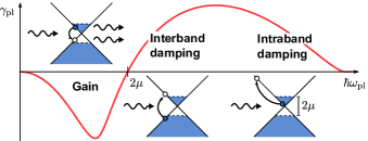
Figure 1: Plasmon decay rate $\gamma_{\mathrm{pl}}$ over plasmon energy $\hbar\omega_{\mathrm{pl}}$ for inverted intrinsic graphene. At energies below $2\mu$ (where $\mu$ is the chemical potential of particles and holes) plasmons undergo stimulated emission processes, accompanied by interband recombination of carriers. Above energies of $2\mu$ stimulated absorption processes associated with inter- and intraband recombination of particle/hole pairs dominate.

II Non-equilibrium plasmons

Graphene supports two types of plasmons, associated with the longitudinal density-density response and the transverse current-current response of the MDF plasma Wunsch et al. (2006); Principi et al. (2009); Stauber and Gómez-Santos (2010); Pellegrino et al. (2011); Gutiérrez-Rubio et al. (2013). Within the field of plasmonics, these collective excitations are frequently referred to as TM (transverse magnetic) and TE (transverse electric) plasmons according to the polarization of the electromagnetic fields. In contrast to the conventional strongly bound TM plasmons, TE plasmons are weakly bound and can only exist under certain restrictive conditions, such as low temperatures or a high-permittivity environment Gutiérrez-Rubio et al. (2013). For the present study on plasmon gain, we only consider TM-polarized longitudinal plasmons, as these plasmons couple more strongly to the particle/hole plasma Polini et al. (2008); Bostwick et al. (2010) and thus constitute the dominant channel for stimulated and spontaneous emission Nikitin et al. (2011); Stauber and Gómez-Santos (2012).

The dispersion of TM graphene plasmons can be obtained by solving Maxwell’s equations for bound TM waves. For graphene suspended in air, neglecting wave retardation (i.e., $|q|\gg\omega/c$), this gives Stern (1967); Mikhailov and Ziegler (2007); Jablan et al. (2009)

$$1+\frac{iq\sigma_{s}(q,\omega)}{2\varepsilon_{0}\omega}\approx 0\>,$$ (1)

where $\sigma_{s}(q,\omega)$, the non-local sheet conductivity, describes the linear current response to an applied electric field with in-plane wavevector $q$ and frequency $\omega$. The same plasmon dispersion equation can be obtained from linear response theory of 2D electron gases Giuliani and Vignale (2005) where longitudinal plasmons emerge as collective charge density waves, whose dispersion is determined by the zeros of the dielectric function Hasegawa and Watabe (1969); Bruus and Flensberg (2004),

$$\varepsilon(q,\omega)=1-V_{q}\Pi(q,\omega)=0\>,$$ (2)

introducing $V_{q}=e^{2}/(2\varepsilon_{0}q)$ as the bare 2D Coulomb potential and $\Pi(q,\omega)$, the irreducible polarizability. Both eqs. (1) and (2) are assuming a linear response of the carriers to an external excitation. Thus, the non-local linear response functions $\sigma_{s}(q,\omega)$ and $\Pi(q,\omega)$ relate to each other via $\sigma_{s}(q,\omega)=i\omega(e^{2}/q^{2})\Pi(q,\omega)$, as a comparison of eqs. (1) and (2) shows. Assuming a weakly interacting 2D electron gas, the irreducible polarizability is, in random-phase approximation (RPA), replaced by the leading order term. We note that the RPA is a commonly employed (see e.g., ref. Hwang and Das Sarma (2007)) and surprisingly accurate approximation for graphene Hofmann et al. (2014).

In the following we lay out the theory for calculating the exact complex-frequency plasmon dispersion, first for the equilibrium system, and then for arbitrary non-equilibrium carrier distributions.

II.1 Complex-frequency dispersion

One of the main objectives of this work is to determine the gain spectrum of plasmons in photo-inverted graphene. This involves consideration of regimes where plasmons are strongly amplified or damped as they couple to the particle/hole plasma via stimulated emission and absorption processes. We therefore do not make the usual low-loss approximation, which treats the plasmon frequency as a purely real variable and extracts the gain/decay rate perturbatively, but instead seek the exact complex-frequency plasmon dispersion (CFPD), as explained in the following.

Our starting point is eq. (2). In RPA, the irreducible polarizability $\Pi(q,\omega)$ is replaced by its leading order term, the polarizability of the non-interacting particle/hole plasma, which we subsequently refer to as, simply, the polarizability. Assuming an arbitrary (non-equilibrium) distribution $n(\epsilon)$ of Dirac fermions, the polarizability is obtained from Stern (1967); Wunsch et al. (2006); Hwang and Das Sarma (2007); Wang and Chakraborty (2007)

$$\Pi[n](q,\omega)=\frac{g}{A}\sum_{s,s^{\prime}=\pm}\sum_{\mathbf{k}}\frac{M_{\mathbf{k},\mathbf{k}+\mathbf{q}}^{ss^{\prime}}\left[n(\epsilon_{\mathbf{k}}^{s})-n(\epsilon_{\mathbf{k}+\mathbf{q}}^{s^{\prime}})\right]}{\epsilon_{\mathbf{k}}^{s}-\epsilon_{\mathbf{k}+\mathbf{q}}^{s^{\prime}}+\hbar\omega+i\times 0}\>,$$ (3)

which describes the bare (unscreened) response of the particle/hole plasma to density fluctuations induced by an external disturbance. The expression is a weighted sum over all intra- and interband transitions $(\mathbf{k},s)\rightarrow(\mathbf{k}+\mathbf{q},s^{\prime})$ where $s=+$ ($s=-$) labels the conduction (valence) band and includes the spin/valley degeneracy in the prefactor $g=4$. Close to the Dirac point, the energy dispersion of the conduction and valence bands is approximately linear ($\epsilon_{\mathbf{k}}^{s}=s\hbar v_{\mathrm{F}}|\mathbf{k}|$) and the square of the transition matrix element is $M_{\mathbf{k},\mathbf{k}^{\prime}}^{ss^{\prime}}=[1+ss^{\prime}\cos(\text{$\theta$}_{\mathbf{k},\mathbf{k}^{\prime}})]/2$ Kotov et al. (2012). The notation $\Pi[n](q,\omega)$ indicates that the polarizability is a functional of the distribution function. In thermal equilibrium, the distribution function $n(\epsilon)$ is given by the Fermi-Dirac distribution, $n(\epsilon)\rightarrow f(\epsilon)|_{\mu}^{T}=1/(\exp[(\epsilon-\mu)/(k_{B}T)]+1)$, parametrized by the chemical potential $\mu$ and temperature $T$; and we define $\Pi|_{\mu}^{T}:=\Pi[f(\circ)|_{\mu}^{T}]$ for brevity. At zero temperature, closed-form expressions have been derived for the equilibrium polarizability Wunsch et al. (2006); Hwang and Das Sarma (2007); Pyatkovskiy (2009), while for finite temperatures it reduces to a semi-analytical form Ramezanali et al. (2009).

For real wavevectors $q$, the complex frequency zeros of eq. (2) define the CFPD $\omega(q)=\omega_{\mathrm{pl}}(q)-i\gamma_{\mathrm{pl}}(q)$, whose real part $\omega_{\mathrm{pl}}(q)$ is the frequency dispersion and imaginary part $\gamma_{\mathrm{pl}}(q)$ is the temporal decay rate. Per definition a negative decay rate implies plasmon gain. Finding the complex-frequency solution requires a polarizability function that is well-defined on the complex frequency plane. The expressions given in refs. Wunsch et al. (2006); Hwang and Das Sarma (2007); Ramezanali et al. (2009), for example, are restricted to real $q$ and $\omega$ as they are defined piecewise or contain Heaviside functions which have no unique complex representation. In regimes where plasmons do not couple to the particle/hole plasma, this is not a problem as one can assume $\gamma_{\mathrm{pl}}\ll\omega_{\mathrm{pl}}$ and then solve eq. (2) approximately by extrapolating around values on the real frequency axis Pyatkovskiy (2009); Jablan et al. (2009). Using a first order Taylor expansion the approximate frequency dispersion $\omega_{\mathrm{pl}}(q)$ is obtained by solving

$$\mathrm{Re}\left[\varepsilon(q,\omega)|_{\omega=\omega_{\mathrm{pl}}(q)}\right]\approx 0\>,$$ (4)

while the corresponding imaginary part, the decay rate Pyatkovskiy (2009); Fetter and Walecka (2012); Principi et al. (2013), emerges as

$$\gamma_{\mathrm{pl}}(q)\approx\left.\frac{\mathrm{Im}[\Pi(q,\omega)]}{\frac{\partial\mathrm{Re}[\Pi(q,\omega)]}{\partial\omega}}\right|_{\omega=\omega_{\mathrm{pl}}(q)}\>.$$ (5)

In section V we show that the rhs is in fact equivalent to the FGR expression for the net stimulated absorption rate of plasmons. In regimes where $\mathrm{Im}[\Pi(q,\omega_{\mathrm{pl}})]=0$ the decay rate $\gamma_{\mathrm{pl}}$ is zero and the solutions of eq. (4) are exact.

For the purpose of finding the exact plasmon gain/loss spectra, we require an expression for the polarizability that applies to complex frequency values. In ref. Pyatkovskiy (2009) an equation for the zero-temperature equilibrium polarizability is reported, which, for the case of gapless graphene, can be written in compact form,

$$\Pi(q,\omega)|_{\mu}^{T=0} =\frac{g\mu}{8\pi\hbar^{2}v_{\mathrm{F}}^{2}}\tilde{\Pi}\left(\frac{\hbar v_{\mathrm{F}}q}{\mu},\frac{\hbar\omega}{\mu}\right)\>,$$ (6)

where

$$\tilde{\Pi}(\tilde{q},\tilde{\omega})=-4+\tilde{q}^{2}\frac{G^{+}\left(\frac{2+\tilde{\omega}}{\tilde{q}}\right)+G^{-}\left(\frac{2-\tilde{\omega}}{\tilde{q}}\right)}{2\sqrt{\tilde{q}^{2}-\tilde{\omega}^{2}}}$$ (7)

is the dimensionless polarizability function, and $G^{\pm}(z)=z\sqrt{1-z^{2}}\pm i\operatorname{arccosh}(z)$. Here, the chemical potential is assumed to be positive and one imposes $\Pi(q,\omega)|_{-\mu}^{T=0}=\Pi(q,\omega)|_{\mu}^{T=0}$ to reflect particle/hole symmetry. For $\omega\rightarrow\omega+i\times 0$ this equation takes the same values as the equations in refs. Wunsch et al. (2006); Hwang and Das Sarma (2007) assuming that the branch-cuts of $G^{\pm}(z)$ are (as usual) oriented along the negative real axis Pyatkovskiy (2009). However, in contrast to other formulations, eq. (6) is analytic in the entire upper complex-frequency half-plane ($\mathrm{Im}[\omega]>0$) and allows for analytic continuation into the lower half-plane ($\mathrm{Im}[\omega]<0$), where plasmons experience loss.

The dielectric function (2) associated with eq. (6) has a scale invariance that becomes apparent when expressing frequency and wavevector in units of the chemical potential $\mu=\hbar\omega_{F}$ and Fermi-wavevector $k_{F}$. Introducing dimensionless variables $\tilde{\omega}=\omega/\omega_{F}=\hbar\omega/\mu$ and $\tilde{q}=q/k_{F}=\hbar v_{F}q/\mu$ one obtains

$$\varepsilon(\tilde{q},\tilde{\omega})=1-\frac{\alpha_{g}}{\tilde{q}}\tilde{\Pi}(\tilde{q},\tilde{\omega})\>,$$ (8)

where $\alpha_{g}=\alpha_{f}c/v_{F}\approx 300/137$ is the effective fine-structure constant of graphene in air Jang et al. (2008); Hofmann et al. (2014). As the solutions of the dispersion relation (8) no longer explicitly depend on the chemical potential, they can be represented by a single plasmon dispersion curve $\tilde{\omega}(\tilde{q})$. This is a result of the conical Dirac dispersion which remains invariant when rescaling energy and momentum variables by the same factor.

To obtain the CFPD we solve eq. (2) numerically using a complex root finding algorithm (Newton-Raphson). Before tracing the dispersion curves we rotate the branch-cuts by $\pm\pi/2$ making them point down into the lower frequency half-plane. Starting from $q=0$ and $\omega=0+i\times 0$ we find the next point of the dispersion by solving eq. (2). Whenever $\omega$ enters the half-space the branch-cuts occupy, we rotate each branch-cut by $\pm\pi$, depending from which side its branch-point is passed, so that they now lie in the opposite half-space. This procedure is repeated as we scan through $q$ and ensures that the complex-frequency dispersion curve $\omega(q)$ never crosses a branch-cut and thus retains a continuous, physical behavior throughout the entire wavevector regime.

In the following we explain how we can generalize the polarizability to finite temperatures and non-equilibrium carrier distributions.

II.2 Non-equilibrium polarizability

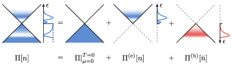
Figure 2: The dynamic polarizability $\Pi[n]$ of an arbitrary non-equilibrium carrier distribution $n(\epsilon)$ can be represented as the sum of the intrinsic zero-temperature polarizability $\Pi(q,\omega)|_{\mu=0}^{T=0}$ and polarizabilities of the particle and hole plasmas $\Pi^{(e)}[n]$ and $\Pi^{(h)}[\bar{n}]$, where $\bar{n}(\epsilon)=1-n(-\epsilon)$.

The polarizability [eq. (3)] depends on the distribution of carriers and captures their response to electromagnetic excitation. It also enters the expression for the screened Coulomb potential $\bar{V}_{q}=V_{q}/\varepsilon(q,\omega)$ Hill et al. (2009), which in turn affects the interaction processes between charged particles, such as carrier-carrier scattering, Auger recombination, impact ionization and optical phonon scattering. Over recent years, intense efforts have been made to calculate the polarizability of graphene, first in the limit of zero doping and zero temperature González et al. (1994), then for finite doping Wunsch et al. (2006); Hwang and Das Sarma (2007), at finite temperatures Vafek (2006); Ramezanali et al. (2009); Tomadin et al. (2013), and in thermal quasi-equilibrium Tomadin et al. (2013).

Here, we present transformations that allow us to calculate polarizabilities associated with arbitrary non-equilibrium carrier distributions. These transformations are then used to calculate the CFPD of photo-inverted graphene in thermal quasi-equilibrium.

Let us first consider the general case where the carrier distribution is not in thermal equilibrium (see fig. 2), but of arbitrary form $n(\epsilon)$. As the polarizability $\Pi=\Pi[n]$, eq. (3), is a linear functional of the non-equilibrium carrier distribution function $n(\epsilon)$ it fulfills the property

$$\Pi[n]=\int_{-\infty}^{+\infty}\mathrm{d}\epsilon\,\Pi[\delta(\epsilon-\circ)]n(\epsilon)\>.$$ (9)

where ‘$\circ$’ marks the variable to which the functional applies. For brevity we here omit the wavevector/frequency arguments [see eq. (3)]. The Dirac-delta function $\delta(\mu-\epsilon)$ can be represented as the derivative of the Fermi-Dirac distribution $f(\epsilon)|_{\mu}^{T}$ in the zero-temperature limit. This allows us to deduce the generic formula,

$$\Pi[n]=\int_{-\infty}^{+\infty}\mathrm{d}\epsilon\,\frac{\partial\Pi|_{\mu=\epsilon}^{T=0}}{\partial\epsilon}n(\epsilon)\>,$$ (10)

for the non-equilibrium polarizability, where $\Pi|_{\mu}^{T=0}=\Pi[f(\circ)|_{\mu}^{T=0}]$ denotes the zero-temperature polarizability associated with the equilibrium distribution of carriers with chemical potential $\mu$. Alternatively, using integration by parts, one may cast eq. (10) into the form

$$\Pi[n]=-\int_{-\infty}^{+\infty}\mathrm{d}\epsilon\,\Pi|_{\mu=\epsilon}^{T=0}\frac{\partial n(\epsilon)}{\partial\epsilon}\>,$$ (11)

where we assumed that $n(\epsilon\rightarrow\infty)=0$ (no occupied states at infinite energy) and $\Pi|_{\mu\rightarrow-\infty}^{T=0}=0$. We justify the latter by inspection of eq. (3). As $\mu\rightarrow-\infty$ the distribution functions necessarily vanish as the (finite) valence band becomes empty. This limit is not reflected in the closed-form expression for the zero-temperature polarizability [eq. (6)], where the integration over energy states is assumed to extend to infinity and has been carried out before the limit $\mu\rightarrow-\infty$ is applied.

As the derivation of eq. (10) is solely based on the linearity of the response function $\Pi[n]$ it is universally applicable to any bandstructure and carrier distribution. It should be noted, that the linearity only holds within the RPA and corrections due to self-interactions, which alter the electronic band structure, are not included. For graphene, the combination of eqs. (6) and (10) proves particularly useful as it enables the numerical evaluation of finite-temperature and non-equilibrium polarizabilities for complex frequencies via analytic continuation.

Owing to graphene’s vanishing band-gap, eq. (10) can be separated into integrals over positive and negative energies. Introducing the hole distribution function $\bar{n}(\epsilon)=1-n(-\epsilon)$ and exploiting particle/hole symmetry, we cast eq. (10) into the following elegant form,

$$\begin{split}\Pi[n]&=\Pi|_{\mu=0}^{T=0}+\\ &\quad\int_{0}^{\infty}\mathrm{d}\epsilon\,\left[\frac{\partial\Pi|_{\mu=\epsilon}^{T=0}}{\partial\epsilon}n(\epsilon)+\frac{\partial\Pi|_{\mu=\epsilon}^{T=0}}{\partial\epsilon}\bar{n}(\epsilon)\right]\\ &=\Pi|_{\mu=0}^{T=0}+\Pi^{(e)}[n]+\Pi^{(h)}[\bar{n}]\>.\end{split}$$ (12)

The non-equilibrium polarizability can thus be represented as the sum of the zero-temperature intrinsic polarizability $\Pi|_{\mu=0}^{T=0}$ and contributions $\Pi^{(e)}[n]$ and $\Pi^{(h)}[\bar{n}]$ for the particles and holes as depicted in fig. 2. This formulation is used later in this work when calculating the plasmon dispersion of photo-inverted graphene at finite temperatures.

The theory presented in this section provides a simple yet powerful tool for the evaluation of the dielectric function for an arbitrary non-equilibrium carrier distribution $n(\epsilon)$. Although we apply it here to find the plasmon dispersion of graphene when the MDF plasma is in an inverted quasi-equilibrium state, it may equally aid the evaluation of the screened Coulomb interaction in MDF plasmas far from thermal equilibrium.

III Plasmons of photo-inverted graphene

The zero-temperature CFPD of extrinsic (doped) graphene in thermal equilibrium has been previously presented in ref. Pyatkovskiy (2009), albeit only inside the Dirac cone ($v_{F}q<\omega$). For photo-inverted graphene the CFPD has, to the best of our knowledge, not yet been studied.

For the rest of this paper we assume a particular non-equilibrium state, known as quasi-equilibrium. The quasi-equilibrium is an approximation that is commonly applied when describing band-gap semiconductors that are pumped into a state of inversion Kesler and Ippen (1987); Haug and Koch (1989). Assuming that carrier-carrier scattering is significantly faster than interband recombination processes, the carriers are able to thermalize within their bands to separate Fermi distributions, each with their own chemical potential. Despite the fact that recombination can be ultrafast in graphene George et al. (2008); Winnerl et al. (2011); Johannsen et al. (2013); Malard et al. (2013); Jensen et al. (2014), carrier-carrier scattering times are still one or two orders of magnitude faster (typically tens of femtoseconds) Dawlaty et al. (2008a); Choi et al. (2009); Breusing et al. (2009, 2011); Malić et al. (2011); Sun et al. (2012). Due to this separation of time-scales, quasi-equilibrium is established some tens of femtoseconds after pulsed excitation. In this context, the derived plasmon dispersion and emission rates are momentary quantities that, together with $\mu_{e}$, $\mu_{h}$, and $T$, evolve in time as the carrier system returns back to equilibrium.

Owing to particle/hole symmetry, carriers thermalize to a common temperature, and the quasi-equilibrium distribution function takes the form

$$n(\epsilon)\rightarrow\theta(\epsilon)f(\epsilon)|_{\mu_{e}}^{T}+\theta(-\epsilon)f(\epsilon)|_{-\mu_{h}}^{T}\>,$$ (13)

where $\mu_{e}$ ($\mu_{h}$) denotes the chemical potential of the Dirac particles (holes).

In order to assess the differences between the plasmon dispersion in equilibrium and the inverted state, we first concentrate on the zero-temperature case, where the expressions for the polarizabilities take closed-form. Inserting the zero-temperature quasi-equilibrium distribution function

$$n(\epsilon)|_{\mu_{e},\mu_{h}}^{T=0}=\theta(\epsilon)\theta(\mu_{e}-\epsilon)+\theta(-\epsilon)\theta(-\mu_{h}-\epsilon)$$ (14)

into eq. (11) yields the expression

$$\begin{split}\Pi(q,\omega)|_{\mu_{e},\mu_{h}}^{T=0}=&\Pi(q,\omega)|_{\mu=0}^{T=0}+\\ &\sum_{\alpha=e,h}\theta(\mu_{\alpha})\left[\Pi(q,\omega)|_{\mu_{\alpha}}^{T=0}-\Pi(q,\omega)|_{\mu=0}^{T=0}\right]\>,\end{split}$$ (15)

where the zero-temperature equilibrium case can be recovered by setting $\mu_{h}=-\mu_{e}$.

In the following, we first study the plasmon dispersion of photo-inverted intrinsic graphene ($\mu_{e}=\mu_{h}>0$) and compare the result with the equilibrium plasmon dispersion of extrinsic graphene ($\mu_{\mathrm{e}}=-\mu_{\mathrm{h}}>0$). The plasmon dispersion in the more general case of photo-inverted extrinsic graphene ($\mu_{e}\neq\mu_{h}$) is examined thereafter.

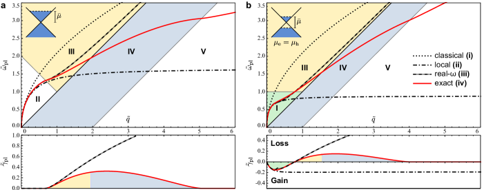
Figure 3: Plasmon frequency dispersion (top panel) and decay rate (bottom panel) for (a) the equilibrium case ($\mu_{e}=-\mu_{h}=\bar{\mu}$) and (b) the photo-inverted intrinsic case ($\mu_{e}=\mu_{h}=\bar{\mu}/2$), using dimensionless variables for frequency $\tilde{\omega}_{\mathrm{pl}}=\hbar\omega_{\mathrm{pl}}/\bar{\mu}$, decay rate $\tilde{\gamma}_{\mathrm{pl}}=\hbar\gamma_{\mathrm{pl}}/\bar{\mu}$, and wavevector $\tilde{q}=\hbar v_{F}q/\bar{\mu}$. The exact complex-frequency dispersion (solid red lines) is shown together with the dispersion in the real-frequency approximation (dashed black lines), in the classical Drude limit (dotted black lines) and using the optical conductivity (dash-dotted black lines). The complex-frequency dispersion (solid red lines) crosses through regions of no loss (II and V; white), regions of inter- (III; yellow) and intraband (IV; blue) damping, and, in case (b), through a region of amplification (I; green), characterized by a negative decay rate.

III.1 Photo-inverted intrinsic graphene

Consider the case where intrinsic graphene is optically excited. As particles/holes are generated in pairs, their quasi-equilibrium chemical potentials will be identical (i.e., $\mu_{\mathrm{e}}=\mu_{\mathrm{h}}$) once the carrier plasmas are thermalized within their respective bands. The zero-temperature quasi-equilibrium polarizability [see eq. (15)] thus simplifies to

$$\begin{split}\Pi(q,\omega)|_{\mu,\mu}^{T=0}=&2\Pi(q,\omega)|_{\mu}^{T=0}-\Pi(q,\omega)|_{\mu=0}^{T=0}\end{split}\>.$$ (16)

We insert this expression into the dielectric function (2) and introduce dimensionless variables to remove the explicit dependency on the chemical potential. This allows us to plot a single representative plasmon dispersion curve for the photo-inverted intrinsic case.

Using analytic continuation we calculated the CFPD for both the (doped) equilibrium ($\mu_{e}=-\mu_{h}=\bar{\mu}$) and photo-inverted intrinsic case ($\mu_{e}=\mu_{h}=\bar{\mu}/2$) by tracing the complex-frequency roots of the dielectric function [see eq. (2)]. The corresponding results are shown in fig. 3(a) and (b), respectively. For comparison, we also show in each figure the real-frequency dispersion obtained in the low-loss approximation (dashed black lines); the dispersion in the classical limit using the Drude conductivity (dotted black lines); and the dispersion in the local approximation ($q\rightarrow 0$) using the optical conductivity (dash-dotted black lines). Frequency and wavevector variables are rescaled to dimensionless quantities $\tilde{\omega}=\hbar\omega/\bar{\mu}$ and $\tilde{q}=\hbar v_{F}q/\bar{\mu}$. For small $\tilde{q}$ the solutions converge to the classical limit (dotted black line), as expected.

To highlight the differences between the CFPD and the approximative dispersion curves, we first inspect the plasmon dispersion in equilibrium. As predicted, the CFPD (red line) matches the real-frequency dispersion (dashed black line) within the loss-free regime II. When the CFPD enters regime III it becomes complex-valued with an imaginary part arising from the interband generation of particle/hole pairs (Landau-damping DuBois and Kivelson (1969); Hwang and Das Sarma (2007); Low and Avouris (2014)) and thus begins to deviate from the real-frequency solution. Note, that owing to the $(\tilde{q}^{2}-\tilde{\omega}^{2})^{-1/2}$ singularity in the polarizability [see eq. (6)] the real-frequency dispersion (dashed black line) cannot cross the Dirac cone but asymptotically approaches $\tilde{\omega}=\tilde{q}$ as $\tilde{q}\rightarrow\infty$. The CFPD, in contrast, eludes the Dirac cone singularity due to its lossy character and crosses smoothly from regime III into the intraband excitation regime IV. After reaching its peak within the intraband regime IV, the decay rate starts to decrease as the phase-space for intraband excitation processes shrinks and eventually becomes zero at the point where the dispersion enters the loss-free region (V).

For the photo-inverted intrinsic case [see fig. 3(b)] the plasmon dispersion (solid red line) initially follows the classical limit (dotted black line). In contrast to the equilibrium case, however, plasmons with small $\tilde{q}$ induce particle/hole recombination processes via stimulated emission and thus experience a negative damping, i.e., amplification. Within region (I), the CFPD experiences gain and thus begins to diverge from the other approximative solutions. After reaching its peak value, the gain steadily decreases and eventually becomes zero at $\tilde{\omega}_{\mathrm{pl}}=\hbar\omega_{\mathrm{pl}}/\bar{\mu}=1$. Above this threshold interband recombination processes are no longer possible at $T=0$ due to a lack of carrier inversion. The plasmon dispersion then enters the interband excitation regime III where plasmons are damped due to generation of particle/hole pairs. Again, the CFPD crosses the Dirac cone, passes through the intraband excitation regime IV and exits into the loss-free region (V), where neither inter- nor intraband excitation can take place as energy and momentum conservation cannot be fulfilled simultaneously. We note, that the real-frequency solution already deviates from the CFPD within region (I) in particular when crossing $\tilde{\omega}_{\mathrm{pl}}=1-\tilde{q}$ where the associated decay rate shows a distinct dip. The dispersion derived from the optical conductivity predicts gain in the long-wavelength region ($q\rightarrow 0$) but fails to display a decrease in gain and does not reproduce the loss in region (IV). This is because intraband processes are forbidden in the applied local limit that only allows vertical transitions.

In this section we studied the plasmon dispersion of photo-inverted intrinsic graphene at zero temperature and compared the result with graphene in equilibrium. We briefly summarize the main findings: (1) within the RPA the calculated CFPD curves represents the exact plasmon dispersion, with an imaginary part that reflects the plasmon loss and gain rate; (2) in contrast to the real-frequency (low-loss) approximation it crosses through both inter- and intraband excitation regimes, where plasmons are damped due to stimulated absorption processes; and (3) for photo-inverted graphene plasmons with frequencies lower than $\hbar\omega<2\mu$ can become amplified due to stimulated emission.

We next study the impact of carrier imbalance (i.e., doping) on the plasmon dispersion of photo-inverted extrinsic graphene.

III.2 Photo-inverted extrinsic graphene

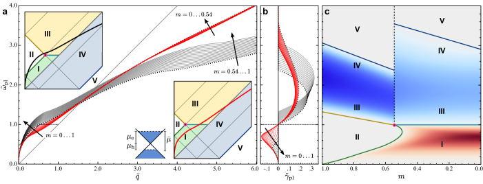
Figure 4: Complex-frequency plasmon dispersion of inverted extrinsic graphene for varying carrier imbalance $m=(\mu_{e}-\mu_{h})/\bar{\mu}$ with $\bar{\mu}=\mu_{e}+\mu_{h}$. (a) Frequency-dispersion curves for $m=0\dots 1$; insets show two representative dispersion curves passing the branch-singularity (filled magenta circle) at the intersection of regions (I)-(III) from above (top left; black line) and below (bottom right; red line). (b) Loss dispersion over plasmon frequency. Dashed curves in (a) and (b) mark solutions with $m$-values just above and below $m_{c}$. (c) decay rate as function of $\omega_{\mathrm{pl}}$ and $m$, depicting gain regions (red), inter-/intraband loss regions (blue) and regions of no loss/gain (grey). The discontinuity (dashed line) originates in the branch-singularity (filled magenta circle). The dimensionless frequency, loss and wavevector are defined by $\tilde{\omega}_{\mathrm{pl}}=\hbar\omega_{\mathrm{pl}}/\bar{\mu}$, $\tilde{\gamma}_{\mathrm{pl}}=\hbar\gamma_{\mathrm{pl}}/\bar{\mu}$, and $\tilde{q}=\hbar v_{F}q/\bar{\mu}$.

Chemical doping or the application of a gate voltage changes the equilibrium carrier density. When pumped into a inverted state, the chemical potentials of particles and holes that characterize the quasi-equilibrium will necessarily differ, i.e., $\mu_{e}\neq\mu_{h}$. Assuming $\mu_{e/h}>0$, eq. (15) simplifies to

$$\begin{split}\Pi(q,\omega)|_{\mu_{e},\mu_{h}}^{T=0}=&\Pi(q,\omega)|_{\mu_{e}}^{T=0}+\Pi(q,\omega)|_{\mu_{h}}^{T=0}\\ &-\Pi(q,\omega)|_{\mu=0}^{T=0}\end{split}\>.$$ (17)

As before, the dispersion equation can be rescaled by introducing appropriate dimensionless variables using the sum of chemical potentials $\bar{\mu}=\mu_{e}+\mu_{\mathrm{h}}$ as a scale parameter. A simple substitution of arguments allows us to recast eq. (17) into the form

$$\Pi(q,\omega)|_{\mu_{e},\mu_{h}}^{T=0}=\frac{g\bar{\mu}}{8\pi\hbar^{2}v_{F}^{2}}\tilde{\Pi}\left.\left(\frac{\hbar v_{\mathrm{F}}q}{\bar{\mu}},\frac{\hbar\omega}{\bar{\mu}}\right)\right|_{m}\>,$$ (18)

where

$$m=\frac{\mu_{e}-\mu_{h}}{\mu_{e}+\mu_{h}}$$ (19)

is the carrier imbalance parameter. The expression for the so-defined dimensionless polarizability

$$\begin{split}\tilde{\Pi}(\tilde{q},\tilde{\omega})|_{m}&=\frac{1+m}{2}\tilde{\Pi}\left(\frac{2\tilde{q}}{1+m},\frac{2\tilde{\omega}}{1+m}\right)\\ &+\frac{1-m}{2}\tilde{\Pi}\left(\frac{2\tilde{q}}{1-m},\frac{2\tilde{\omega}}{1-m}\right)\\ &-\lim_{x\rightarrow 0}x\tilde{\Pi}\left(\frac{\tilde{q}}{x},\frac{\tilde{\omega}}{x}\right)\end{split}$$ (20)

contains the equilibrium polarizability $\tilde{\Pi}(\tilde{q},\tilde{\omega})$ as defined in eq. (6). The last term is the intrinsic polarizability, which, as a consequence of the scaling, now appears in the limit $x\rightarrow 0$.

The parameter $m$ quantifies the relative difference of the chemical potentials of particles and holes. A value of $m=0$ represents the photo-inverted intrinsic case; $m=\pm 1$ the doped equilibrium cases where only one plasma component is excited; and values in between, the general case. Owing to particle/hole symmetry, eq. (20) only depends on $|m|$ and we can restrict ourselves to positive values of $m$ without loss of generality.

Figure 4(a) depicts the calculated frequency dispersion curves $\omega_{\mathrm{pl}}(q)$ for varying values of $m$. As the plasmon frequency dispersion curves are strictly monotonic, we can express the loss dispersion $\tilde{\gamma}_{\mathrm{pl}}(q)$ as function of frequency, i.e., $\tilde{\gamma}_{\mathrm{pl}}(\tilde{\omega}_{\mathrm{pl}})=\tilde{\gamma}_{\mathrm{pl}}(\tilde{q}(\tilde{\omega}_{pl}))$ , as shown in fig. 4(b). When varying $m$, all loss spectra pass through zero at $\tilde{\omega}=1$, where the CFPD curves pass from the gain into the loss region. For small frequencies values ($\tilde{\omega}_{\mathrm{pl}}<1$) the dispersion curves form a single bundle [see fig. 4(a)], in the sense that an infinitesimal change of $m$ will lead to an infinitesimal variation of $\tilde{\omega}_{\mathrm{pl}}(\tilde{q})$. One may expect that the solutions undergo a continuous variation when varying the inversion parameter $m$. Instead, the plasmon dispersion curves split into two bundles at $\tilde{\omega}_{\mathrm{pl}}=1$, cross-over and become well separated at larger frequencies/wavevectors. The first bundle (solid red lines) contains dispersion curves with $m=0\ldots m_{c}$, where $m_{c}\approx 0.538$. Dispersion curves in this bundle make a direct transition from the trapezoidal gain region (I) into the lossy interband excitation region (III). The second bundle (solid black lines), comprising dispersion curves with $m=m_{c}\dots 1$, is associated with a large imbalance in particle/hole numbers. These curves start in the gain region (I) but pass through the loss-free region (II) before entering the loss region (III).

A qualitative difference between the low-$m$ and the high-$m$ bundle is that curves in the latter enter region (III) with a zero imaginary part, and therefore glance the branch point which separates the two regions (yellow line), whereas curves in the former bundle avoid it, as prescribed in section II.1.

The split-up of the bundle occurs at the intersection point of regions (I), (II), and (III) [filled magenta circle in fig. 4(a)] where the polarizability has a degenerate branch-singularity. The critical value $m_{c}$ is calculated by finding the dispersion curve that passes through this branch-singularity, i.e., from the condition

$$1-\frac{\alpha_{g}}{\tilde{q}}\tilde{\Pi}(m_{c},1)|_{m_{c}}=0\>.$$ (21)

Note, that while the plasmon dispersion curves are continuous (and smooth) in $\tilde{q}$, a change in $m$ does not necessarily cause a continuous variation of the curves. Adjacent curves can flank the branch-singularity from opposite sides and thus end up on different Riemann sheets of the dielectric function (2) giving rise to the observed splitting of the bundle. This is most evident from fig. 4(b) where the loss dispersion curves are separated into two bundles just above $\tilde{\omega}_{\mathrm{pl}}=1$ and then follow distinct trends.

The plasmon decay rate $\tilde{\gamma}_{\mathrm{pl}}$ [see fig. 4(b)] strongly depends on both the plasmon frequency $\tilde{\omega}_{\mathrm{pl}}$ and the carrier imbalance parameter $m$. For frequencies below (above) $\tilde{\omega}_{\mathrm{pl}}=1$, plasmon amplification (damping) occurs as indicated by red (blue) curves in fig. 4(c). At $m=0$ (intrinsic inverted case) the gain spectrum features a single broad peak. As $m$ increases this peak first red shifts and then splits into two peaks, which, for even larger values of $m$, become separated by a loss-free frequency region. For values of $m$ larger than $m_{c}$ the second peak vanishes and the loss-free region extends in frequency, reducing the gain available at low frequencies until the loss-free region (II) covers the whole frequency range $\tilde{\omega}_{\mathrm{pl}}<1$ when $m\rightarrow 1$ (doped equilibrium case). The discontinuity in $m$ stretches out from the branch-singularity at $m=m_{c}$ towards frequencies $\tilde{\omega}_{\mathrm{pl}}>1$ (dashed line). It should be pointed out that this discontinuity is rooted in the singularities of the polarizability, which are physical and cannot be lifted. As the polarizability appears in the Helmholtz free energy Vafek (2007); Ramezanali et al. (2009); Faridi et al. (2012) the discontinuity may relate to a thermodynamic phase-transition. This clearly requires a more in depth analysis, which goes beyond the scope of this paper and will be explored in a follow-up study.

Concluding this section, we briefly summarize the main findings: (1) The complex-frequency solutions of the dispersion equation deliver a consistent picture of the frequency and loss dispersion of plasmons; (2) Plasmons are amplified in photo-inverted graphene at frequencies $\hbar\omega_{pl}<\mu_{e}+\mu_{h}$ due to stimulated emission; and (3) The plasmon gain spectrum is strongly influenced by the carrier imbalance parameter $m=(\mu_{e}-\mu_{h})/(\mu_{e}+\mu_{h})$, exhibiting discontinuous behavior at $m\approx 0.538$ when the plasmon dispersion passes through a singularity.

IV Collision loss and temperature

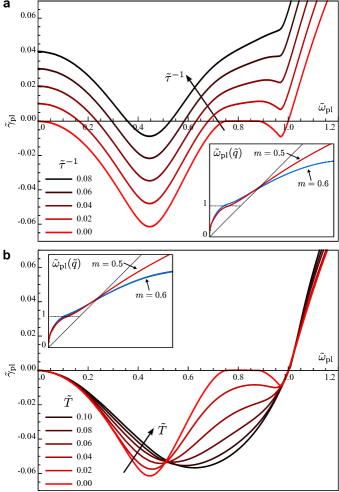
Figure 5: Impact of temperature and collision loss on plasmon decay rate and frequency dispersion. (a) Plasmon decay rate at $m=0.5$ for collision loss rates ranging from $\tilde{\tau}^{-1}=0$ to $\tilde{\tau}^{-1}=0.08$ , where $\tilde{\tau}^{-1}=\hbar\tau^{-1}/\bar{\mu}$. (b) Plasmon decay rate at $m=0.5$ for temperatures ranging from $\tilde{T}=0$ (red lines) to $\tilde{T}=0.1$ (black lines), where $\tilde{T}=k_{B}T/\bar{\mu}$. Insets display the corresponding frequency dispersion curves for $m=0.5$ (red lines) and $m=0.6$ (blue lines).

So far, all calculations have been carried out under the idealized assumptions of zero temperature and without the inclusion of collision loss. In this section we aim to clarify how finite-temperatures and collision losses impact on the spectral characteristics of plasmon gain in photo-inverted graphene.

IV.1 Impact of collision loss

Without the inclusion of collision losses, equilibrium plasmons are completely loss-free within regions (II) and (V) of figs. 2 and 4, where the Landau damping is suppressed. In reality, collisions with impurities, acoustic phonons and optical phonons Yan et al. (2013) limit the life-time and propagation length of graphene plasmons, with a collision time $\tau$ that can range from tens to hundreds of femtoseconds depending on the quality of the sample Dawlaty et al. (2008a, b) and substrate used Scharf et al. (2013).

To theoretically assess the effect of carrier collisions (quantified by the phenomenological rate $\tau^{-1}$) on the plasmon dispersion and loss we impose the transformation Mermin (1970)

$$\Pi_{\tau}(q,\omega)=\frac{(\omega+i\tau^{-1})\text{$\Pi$}(q,\omega+i\tau^{-1})}{\omega+i\tau^{-1}\Pi(q,\omega+i\tau^{-1})/\Pi(q,0)}$$ (22)

on the polarizability $\text{$\Pi$}(q,\omega)$, which, in contrast to a simple replacement $\text{$\Pi$}_{\tau}(q,\omega)=\text{$\Pi$}(q,\omega+i\tau^{-1})$, conserves particle numbers locally. In cases where $\text{$\Pi$}(q,\omega)$ only accepts real frequency values, a Taylor expansion $\text{$\Pi$}(q,\omega+i\tau^{-1})=\text{$\Pi$}(q,\omega)+i\tau^{-1}\partial\text{$\Pi$}(q,\omega)/\partial\omega$ needs to be carried out, effectively limiting the validity of eq. (22) to small collision rates $\tau^{-1}$ Jablan et al. (2009). This limitation does not exist when using eq. (6) in conjunction with the non-equilibrium polarizabilities, such as eq. (17). Their validity extends to the complex frequency plane and thus permits a direct application of the transformation (22).

In solving eq. (2) together with eq. (22) we directly obtain the CFPD for the photo-inverted case with collision losses. Figure 5(a) depicts the plasmon gain spectrum for a carrier imbalance of $m=0.5$. The collision rates are varied from $\tilde{\tau}^{-1}=0$ to $\tilde{\tau}^{-1}=0.08$ ($\tilde{\tau}^{-1}=\hbar\tau^{-1}/\bar{\mu}$). The maximum value corresponds to a collision time of only $\tau=20\,\mathrm{fs}$ at an inversion of $\bar{\mu}=0.2\,\mathrm{eV}$. We observe that the collision time only moderately affects the shape of the loss dispersion curve and that, at each given frequency, the decay rate $\tilde{\gamma}_{\mathrm{pl}}(\tilde{\omega}_{\mathrm{pl}})$ is proportional to $\tau^{-1}$ [see fig. 5(a)]. At the highest collision rate of $\tilde{\tau}^{-1}=0.08$ there is still a frequency region where plasmons are amplified (i.e., have a negative decay rate). Eventually, for even higher collision rates, interband gain will no longer be able to compensate the collision loss and the plasmons will become lossy across the entire frequency spectrum. Surprisingly, the frequency dispersion is almost unaffected by the introduction of collision loss as can be seen from the bundle of dispersion curves $\tilde{\omega}_{\mathrm{pl}}(\tilde{q})$, which come to lie on top of each other when varying the collision rate [see red lines in inset of fig. 5(a)].

We finally note, that the splitting of the dispersion bundle observed in section III is robust against the introduction of collision loss and occurs roughly at the same critical value of $m_{c}\approx 0.538$. To give evidence for this behavior we show the dispersion curves associated with a value of $m=0.6$ (blue lines) in the inset of fig. 5(a), which clearly belong to the high-$m$ bundle and thus follow a different path than those for $m=0.5$ (red lines).

IV.2 Finite-temperature

The influence of temperature on the plasmon dispersion of graphene has first been analyzed in ref. Ramezanali et al. (2009), where a semi-analytical formula for the finite-temperature polarizability has been derived. Here, we seek a formulation that applies to photo-inverted graphene in thermal quasi-equilibrium and is valid for complex frequencies.

We employ eq. (12), which, owing to the linear character of the functionals, can be cast into the form

$$\Pi|_{\mu_{e},\mu_{h}}^{T}=\Pi|_{\mu_{e},\mu_{h}}^{T=0}+\Pi^{(e)}[\delta f|_{\mu_{e}}^{T}]+\Pi^{(h)}[\delta f|_{\mu_{h}}^{T}]\>,$$ (23)

where

$$\delta f(\epsilon)|_{\mu}^{T}=f(\epsilon)|_{\mu}^{T}-f(\epsilon)|_{\mu}^{T=0}.$$ (24)

In this expression the zero-temperature quasi-equilibrium $\Pi|_{\mu_{e},\mu_{h}}^{T=0}$ is augmented by corrections that capture the change of the polarizability due to smearing of the Fermi-edge as quantified by $\delta f(\epsilon)|_{\mu}^{T}$. This corrective approach enables us to trace the CFPD at finite temperatures with high accuracy. The evaluation of eq. (23) requires the derivative of the polarizability (6), which is given by the following closed-form expression

$$\frac{\partial\Pi(q,\omega)|_{\mu}^{T=0}}{\partial\mu} =\frac{g}{8\pi\hbar^{2}v_{F}^{2}}\tilde{\Pi}^{\prime}\left(\frac{\hbar v_{F}q}{\mu},\frac{\hbar\omega}{\mu}\right)\>,$$ (25)

where

$$\tilde{\Pi}^{\prime}(\tilde{q},\tilde{\omega})=-4+2\tilde{q}\frac{G^{\prime}\left(\frac{2+\tilde{\omega}}{\tilde{q}}\right)+G^{\prime}\left(\frac{2-\tilde{\omega}}{\tilde{q}}\right)}{\sqrt{\tilde{q}^{2}-\tilde{\omega}^{2}}}$$ (26)

and $G^{\prime}(z)=\sqrt{1-z^{2}}$. Just as eq. (6), the equation above is analytic on the upper frequency half-plane and thus reproduces the correct values for real frequencies when using the prescription $\omega\rightarrow\omega+i\times 0$. Note, that the positions of the branch cuts of $\partial\Pi(q,\omega)|_{\mu}^{T=0}/\partial\mu$ vary with the integration variable (i.e., the chemical potential $\mu$) in eq. (12). The analytic continuation needs to be carried out inside the integrals as the CFPD traverses the complex plane.

Solving eq. (2) together with eqs. (23)-(26) gives the finite-temperature CFPD curves, plotted in fig. 5(b) for $m=0.5$ and temperatures $\tilde{T}=k_{B}T/\bar{\mu}$ ranging from $\tilde{T}=0$ (red line) to $\tilde{T}=0.1$ (black line). Assuming $\bar{\mu}=0.2\,\mathrm{eV}$ this translates to a temperature range of $T=0-232.1\,\mathrm{K}$. We first note that the loss curves $\tilde{\gamma}_{\mathrm{pl}}(\tilde{\omega}_{\mathrm{pl}})$ associated with different temperatures all pass through zero at $\tilde{\omega}=1$. With temperatures $\tilde{T}\ll 1$ the smearing of the Fermi-edges does seemingly not impact the point where stimulated emission and absorption processes are balanced. For frequencies below $\tilde{\omega}=1$ the plasmon gain is strongly affected by temperature, displaying a distinctive blue-shift of the gain peak with increasing temperature. In addition, the region of zero gain/loss that occurs for $\tilde{T}=0$ at around $\tilde{\omega}=0.8$ vanishes for finite temperature leading to a strongly broadened gain spectrum. Although the shape of the gain spectrum is strongly affected by temperature, the frequency dispersion $\tilde{\omega}_{\mathrm{pl}}(\tilde{q})$ remains fairly unaffected [see red lines in 5(b)], just as in the case of collision loss.

The splitting behavior observed in section III for the idealized case (zero-temperature and zero collision loss) proves to be remarkably robust against temperature as can be seen from the second set of dispersion curves (5b; blue lines), which for $m=0.6$ follow a different trajectory. The critical value $m_{c}$ at which the splitting occurs shifts slightly towards larger values and is found to be $m_{c}\approx 0.56$ for $\tilde{T}=0.1$ compared to $m_{c}\approx 0.538$ at $\tilde{T}=0$.

For a more realistic description of the plasmon dispersion, one may wish to include both finite collision loss and finite temperature. The procedure for this is straight-forward: First one applies eq. (22) to obtain the equilibrium polarizability with finite collision loss and thereafter the transformation (23) to generalize for a finite temperature.

V Spontaneous plasmon emission spectra

The calculated CFPD curves account for both the frequency and loss dispersion of the plasmons. The losses and gain in regimes I, III and IV of fig. 3, due to single particle excitation, can be related to the three fundamental processes of light-matter interaction: absorption, stimulated emission and spontaneous emission. In photo-inverted graphene, at frequencies below $\hbar\omega_{\mathrm{pl}}<\bar{\mu}$, plasmons experience gain due to stimulated emission processes and thus acquire a negative decay rate $\gamma_{\mathrm{pl}}$ (region (I) in fig. 3). Considering the situation where all plasmon modes are in their ground state, the rate of spontaneous plasmon emission into a frequency interval $[\omega,\omega+\mathrm{d}\omega]$ is equal to the stimulated emission rate weighted with the plasmon density of states. In the following, we extract the spontaneous plasmon emission spectra from the CFPDs, compare them with first order approximative results obtained from Fermi’s golden rule (FGR), and calculate the total spontaneous carrier recombination rates.

For the following interpretation it is instructive to draw the connection between FGR for plasmon emission and eq. (5). Within the semiclassical framework the decay of plasmon population due to stimulated processes can be expressed as

$$\frac{\partial n_{\mathrm{pl}}(q)}{\partial t}=-\gamma_{\mathrm{pl}}^{\mathrm{stim}}(q)n_{\mathrm{pl}}(q)\>,$$ (27)

where the net stimulated absorption rate $\gamma_{\mathrm{pl}}^{\mathrm{stim}}(q)$ is the stimulated absorption minus the stimulated emission rate. As $\gamma_{\mathrm{pl}}^{\mathrm{stim}}(q)$ is an intensity related quantity, it is twice the plasmon decay rate, i.e.,

$$\gamma_{\mathrm{pl}}^{\mathrm{stim}}(q)=2\gamma_{\mathrm{pl}}(q)\>.$$ (28)

In cases where $\gamma_{\mathrm{pl}}\ll\omega_{\mathrm{pl}}$ the plasmon decay rate is approximated to first order by eq. (5). Inserting the imaginary part of the polarizability (3)

$$\begin{split}\mathrm{Im}[\Pi(q,\omega)]=&\frac{\pi}{\hbar}\frac{g}{A}\sum_{s,s^{\prime}=\pm}\sum_{\mathbf{k}}\hbar\delta(\hbar\omega+\epsilon_{\mathbf{k}}^{s}-\epsilon_{\mathbf{k}+\mathbf{q}}^{s^{\prime}})\\ &\times M_{\mathbf{k},\mathbf{k}+\mathbf{q}}^{ss^{\prime}}\left[f(\epsilon_{\mathbf{k}}^{s})-f(\epsilon_{\mathbf{k}+\mathbf{q}}^{s^{\prime}})\right]\end{split}$$ (29)

into eq. (5) reproduces the FGR expressions for the stimulated intra- and interband processes (see also ref. Rana et al. (2011)). In applying the identity $f-f^{\prime}=f(1-f^{\prime})-f^{\prime}(1-f)$ to the difference of Fermi functions in eq. (29), one can then split the net stimulated rate into rates for the absorption and emission processes. Focusing on interband emission processes we thus identify the FGR expression associated with the emission of plasmons

$$\begin{split}g_{\mathrm{pl}}(q)\approx&\frac{2\pi}{\hbar}\frac{g}{A}\sum_{\mathbf{k}}\hbar\delta(\hbar\omega_{\mathrm{pl}}(q)-\epsilon_{\mathbf{k}}-\epsilon_{\mathbf{k}+\mathbf{q}})\\ &\times M_{\mathbf{k},\mathbf{k}+\mathbf{q}}^{-+}f(\epsilon_{\mathbf{k}+\mathbf{q}})|_{\mu_{e}}^{T}f(\epsilon_{\mathbf{k}})|_{\mu_{h}}^{T}\\ &\times\left.\frac{V_{q}}{\frac{\partial\mathrm{Re}[\varepsilon(q,\omega)]}{\partial\omega}}\right|_{\omega=\omega_{\mathrm{pl}}(q)}\>,\end{split}$$ (30)

where $\epsilon_{\mathbf{k}}=\epsilon_{\mathbf{k}}^{+}$. To evaluate this expression, the sum over $\mathbf{k}$-states is replaced by an integration over momentum space. After performing a series of algebraic transformations, detailed in appendix A, we find the following semi-analytical equation for the plasmon emission rate:

$$\begin{split}g_{\mathrm{pl}}(q)\approx&\alpha_{f}cq\frac{\theta(\omega-v_{F}q)}{\sqrt{\omega^{2}-(v_{F}q)^{2}}}\frac{2K(q,\omega)}{\frac{\partial\mathrm{Re}[\varepsilon(q,\omega)]}{\partial\omega}}\Biggr{|}_{\omega=\omega_{\mathrm{pl}}(q)}\>.\end{split}$$ (31)

The function $K(q,\omega)$, a measure for the phase-space associated with the emission processes, is defined as

$$\begin{split}K(q,\omega)=&\int\limits_{-1}^{\mbox{\mbox{+1}}}\mathrm{d}u\>\sqrt{1-u^{2}}\\ &\qquad\times f(\hbar(\omega+v_{F}qu)/2)|_{\mu_{e}}^{T}\\ &\qquad\times f(\hbar(\omega-v_{F}qu)/2)|_{\mu_{h}}^{T}\>.\end{split}$$ (32)

It is clear from the calculation above that FGR (30) is an first order approximation in $\gamma_{\mathrm{pl}}/\omega_{\mathrm{pl}}$ that is accurate as long as the plasmon loss/gain rates are much smaller than the plasmon frequency.

From the plasmon emission rate $g_{\mathrm{pl}}(q)$ one can derive the plasmon emission spectrum $G_{\mathrm{pl}}(\omega)$ as follows: Summation of $g_{\mathrm{pl}}(q)$ over all wavevector states defines the spontaneous plasmon emission rate

$$\begin{split}R_{\mathrm{pl}}^{\mathrm{\mathrm{spon}}}&=\frac{1}{A}\sum_{\mathbf{q}}g_{\mathrm{pl}}(q)=\int\limits_{0}^{\infty}\,\mathrm{d}\omega\,G_{\mathrm{pl}}(\omega)\>,\end{split}$$ (33)

which in turn is obtained by integrating the plasmon emission spectrum $G_{\mathrm{pl}}(\omega)$ over frequency. From the equation above it is clear that the plasmon emission spectrum $G_{\mathrm{pl}}(\omega)$ is just

$$G_{\mathrm{pl}}(\omega)=D_{\mathrm{pl}}(\omega)g_{\mathrm{pl}}(q(\omega))\>,$$ (34)

where the plasmon density of states

$$D_{\mathrm{pl}}(\omega)=\frac{q(\omega)}{2\pi}\frac{\mathrm{d}q(\omega)}{\mathrm{d}\omega}\>$$ (35)

quantifies how many plasmons per unit area and time are spontaneously emitted into the (infinitesimal) frequency-interval $[\omega,\omega+\mathrm{d}\omega]$.

Dividing the spontaneous plasmon emission rate $R_{\mathrm{pl}}^{\mathrm{spon}}$ by the particle area density yields the recombination rate

$$\Gamma_{\mathrm{pl}}^{(e)}=R_{\mathrm{pl}}^{\mathrm{spon}}/N(\mu_{e},T)$$ (36)

where $N(\mu_{\mathrm{e}},T)$ is the area density of MDFs in the conduction band.

Carrier recombination rates due to plasmon emission have been previously calculated in ref. Rana et al. (2011) using FGR with the limitation that only the intraband contribution of the polarizability to the plasmon dispersion had been taken into account. The reported rates suggest that plasmon emission is an ultrafast channel for carrier recombination that needs to be considered when analyzing the hot carrier dynamics in graphene Breusing et al. (2011); Li et al. (2012); Gierz et al. (2013).

In the following, we determine the exact plasmon emission spectra and recombination rates directly from the CFPD and compare the result with approximative solutions obtained from FGR. With the exact solution as a benchmark, we are able to assess the limitations of FGR, which as we will show, depends on the accuracy of the plasmon dispersion used for its evaluation.

V.1 Plasmon emission at zero temperature

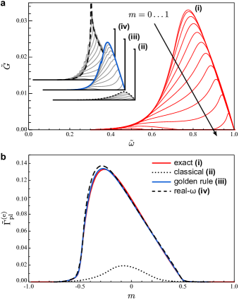
Figure 6: Spontaneous plasmon emission spectra $\tilde{G}_{\mathrm{pl}}(\omega)$ (a) and electron recombination rates $\tilde{\Gamma}_{\mathrm{pl}}^{(e)}$ (b) at zero temperature and in dependence of carrier imbalance $m$. The respective dimensionless quantities are defined as $\tilde{G}_{\mathrm{pl}}=(\hbar v_{F})^{2}G_{\mathrm{pl}}/\bar{\mu}^{2}$ and $\tilde{\Gamma}_{\mathrm{pl}}^{(e)}=\hbar\Gamma_{\mathrm{pl}}^{(e)}/\bar{\mu}$ (see appendix B). Exact results (i) derived from the exact complex-$\omega$ plasmon dispersion curves, together with approximative results obtained from Fermi’s golden rule in conjunction with (ii) the classical (Drude) dispersion, (iii) the complex-$\omega$ dispersion, and (iv) the real-$\omega$ dispersion.

At zero temperature the Fermi-surfaces of the particle/hole plasmas are sharply defined. Depending on the frequency, the graphene plasmons will either experience gain ($\hbar\omega_{\mathrm{pl}}<\bar{\mu}$) or loss ($\hbar\omega_{\mathrm{pl}}>\bar{\mu}$) as shown in fig. 4. It is also clear from fig. 4 that for $\hbar\omega_{pl}<\bar{\mu}$ plasmons only exist left of the Dirac cone where intraband processes cannot occur. This implies that for $\hbar\omega_{\mathrm{pl}}<\bar{\mu}$ plasmons are only subjected to emission processes and we can write

$$\begin{split}g_{\mathrm{pl}}(q)&=-\theta(\bar{\mu}-\hbar\omega_{\mathrm{pl}}(q))\gamma_{\mathrm{pl}}^{\mathrm{stim}}(q)\end{split}$$ (37)

for the plasmon emission rate. As $\gamma_{\mathrm{pl}}^{\mathrm{stim}}(q)=2\gamma_{\mathrm{pl}}(q)$ we can determine the plasmon emission rate $g_{\mathrm{pl}}(q)$ directly from the CFPD curves (see fig. 4) and then calculate the exact plasmon emission spectrum $G_{\mathrm{pl}}(\omega)$ with the help of eq. (34). This also puts us into the position to assess the accuracy of FGR when using different approximations to the plasmon frequency dispersion with the exact result as a reference.

In fig. 6(a) we plot the plasmon emission spectra $\tilde{G}_{\mathrm{pl}}(\omega)$ of photo-inverted extrinsic graphene at zero temperature in dimensionless scaling (see appendix B). The exact result [(i), red lines] is shown together with approximative results, all obtained from FGR [see eq. (31)] using the following different solutions for the frequency dispersion $\omega_{\mathrm{pl}}(q)$: (ii) the approximate dispersion obtained in the classical (Drude) limit of the conductivity (dotted line), (iii) the exact dispersion obtained from the real part of the CFPD (dash-dotted line); and (iv) the real-frequency (low-loss) approximation of the dispersion(dashed line). Of these three emission spectra, the classical approximation is worst, as it severely underestimates the plasmon emission rate, since the plasmon density of states that enters eq. (34) is about a factor of 10 lower in the classical limit. Solution (ii) reproduces the shape of the emission spectrum apart from small deviations (dips) that occur when the plasmon dispersion crosses the boundaries of the regions depicted in fig. 4. Solution (iii) features pronounced spikes, which are induced by the first-order approximation [see eqs. (4) and (5)].

Integrating the emission spectrum $\tilde{G}_{\mathrm{pl}}(\omega)$ over all frequencies gives the spontaneous carrier recombination rate $\tilde{\Gamma}_{\mathrm{pl}}^{(e)}$, which we plot as a function of carrier imbalance $m$. We first note, that while $\tilde{\Gamma}_{\mathrm{pl}}^{(e)}(m)=\tilde{\Gamma}_{\mathrm{pl}}^{(h)}(-m)$ holds due to particle/hole symmetry, the particle recombination rate $\tilde{\Gamma}_{\mathrm{pl}}^{(e)}(m)$ itself is not symmetric in $m$ as the recombination rates are obtained from eq. (36) by dividing the emission rate $\tilde{R}_{\mathrm{pl}}^{\mathrm{spon}}$ by the particle density. As a result, the curves in fig. 6(b) are skewed towards negative $m$-values, indicating that particle/hole recombination is faster for the p-doped case, where holes are the majority carriers. Using the classical approximation (ii) for the dispersion in conjunction with FGR (dotted black line) underestimates the rates by a factor of 5 at m=0. The approximative results (iii) and (iv) reproduce the shape and magnitude of the exact emission rate (i) quite well, apart from a small shift in $m$ towards negative values. This means that the first-order approximation (iv) does provide a good estimate for the carrier recombination rate, despite not reproducing the plasmon emission spectra correctly.

The scale-free representation implies that the emission spectrum $G_{\mathrm{pl}}(\omega)$ scales with $\bar{\mu}^{2}$ and the recombination rate $\Gamma_{\mathrm{pl}}^{(e)}$ with $\bar{\mu}$. The actual values for the carrier recombination rates can be directly extracted from fig. 6(b). Assuming for example an inversion of $\bar{\mu}=0.2\,\mathrm{eV}$ (and $m=0$) the calculated spontaneous recombination times are $34\,\mathrm{fs}$ for the exact solution (i) and $\sim\!187\,\mathrm{fs}$ when using the Drude approximation (ii). The latter is in good agreement with those presented in ref. Rana et al. (2011) (see fig. 5 therein), which are based on FGR and a plasmon dispersion for which only intraband contributions to the polarizability have been considered. This result implies that spontaneous plasmon emission is significantly faster than previously assumed and constitutes an important recombination channel that needs to be considered together with Auger recombination Rana (2007); Winzer and Malić (2012); Tomadin et al. (2013); Brida et al. (2013) and optical phonon emission Butscher et al. (2007); Rana et al. (2009); Wang et al. (2010); Yan et al. (2013).

V.2 Impact of collision loss and temperature

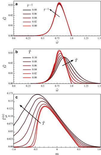
Figure 7: Impact of collision loss and temperature on the plasmon gain spectra. (a) Plasmon gain spectra $\tilde{G}_{\mathrm{pl}}(\tilde{\omega})$ for $m=0$ and collision loss rates ranging from $\tilde{\tau}^{-1}=0$ to $\tilde{\tau}^{-1}=0.08$. (b) Plasmon gain spectra for $m=0$ and temperatures ranging from $\tilde{T}=0$ to $\tilde{T}=0.1$. (c) Particle recombination rates over carrier imbalance parameter $m$ for temperatures from $\tilde{T}=0$ to $\tilde{T}=0.1$. The dimensionless spectral gain and carrier recombination rates are defined as $\tilde{G}_{\mathrm{pl}}=(\hbar v_{F})^{2}G_{\mathrm{pl}}/\bar{\mu}^{2}$ and $\tilde{\Gamma}_{\mathrm{pl}}^{(e)}=\hbar\Gamma_{\mathrm{pl}}^{(e)}/\bar{\mu}$.

We next examine the influence of collision loss and temperature on the plasmon emission spectra and the carrier recombination rates. In contrast to the ideal case (zero-temperature, collision-free) it is not possible to determine the exact emission spectra for finite collision loss or temperature as relation (37) no longer holds under these conditions. However, in the first part of this section we concluded that the combination of FGR and complex-frequency dispersion [(i) and (iii) in Fig. 6] provides a good approximation for both the emission spectra and recombination rates (see fig. 6).

As the collision loss does not enter the FGR expression (31) explicitly and only weakly affects the plasmon dispersion (as shown in section IV), we expect the spontaneous emission spectrum to have a weak dependence on the collision loss rate. Indeed, fig. 7(a) shows that an increase of the collision loss only causes a small increase of the emission spectrum that is most prominent around the emission peak. As a result, we do not observe a significant change of the carrier recombination rate with increasing collision rate, and therefore do not present this.

For finite temperature, the situation is different; the Fermi distribution of the particle/hole plasmas that enter eq. (32) are smeared out. With increasing temperature, the peak gain decreases due to a reduction of the carrier occupation below $\tilde{\omega}=1$ [see fig. 7(b)]. On the other hand, emission processes are now possible above $\tilde{\omega}=1$, which was the zero-temperature limit for spontaneous emission. As a consequence, the spectral gain [see fig. 7(b)] becomes increasingly broadened for increasing temperature, showing both a characteristic blue-shift and reduction of the peak gain. Integrating the emission spectrum gives the total carrier recombination rate, which we show in fig. 7(c) as a function of the carrier imbalance $m$. We observe the recombination rate rises with temperature. The effect is most pronounced around $m\approx-1$ where the particles are minority carriers and the temperature has a strong influence on the number of particles in the conduction band. The peak recombination rate shifts towards more negative values of $m$ as the temperature increases. At $m=0$, the recombination rates are least dependent of the value of $T$ due to the symmetry in the particle/hole population.

As interpretation of fig. 7 we give dimensional quantities for $\bar{\mu}=0.2\mathrm{eV}$. At zero temperature, the spectral gain peaks at $\omega=2.3\times 10^{14}\mathrm{Hz}$ with a value of $G=3.4\times 10^{-16}\mathrm{m}^{2}$ and cuts off sharply at $\omega=3.0\times 10^{14}\mathrm{Hz}$. The curve with $\tilde{T}=0.1$ corresponds to $T=230\mathrm{K}$. The carrier recombination times of $1/\Gamma^{(e)}_{\mathrm{pl}}=34\mathrm{fs}$ for $m=0$, i.e. $\mu_{e}=\mu_{h}=0.1\mathrm{eV}$ at $T=0$, drop to $18\mathrm{fs}$ for $m=-0.5$, i.e. $\mu_{e}=0.05\mathrm{eV}$ and $\mu_{h}=0.15\mathrm{eV}$, for $T=230\mathrm{K}$.

We briefly summarize the main results of this section: (1) A comparison of the plasmon emission spectra at zero temperature shows that the accuracy of Fermi’s golden rule depends critically on the plasmon dispersion with best results when the exact dispersion is inserted; (2) The calculated carrier recombination rates for plasmon emission are more than a factor of 5 larger than those obtained in the classical limit; (3) Collision loss has no influence on the plasmon emission spectra and carrier recombination rates; and (4) An increase in temperature leads to a broadening and blue-shift of the emission spectrum and increases the carrier recombination rates, particularly at a high carrier imbalance, i.e., when $|m|>0.2$.

VI Conclusion

In calculating the gain spectra of photo-inverted graphene self-consistently from the exact complex-frequency dispersion curves, this work provides evidence that graphene can, under realistic conditions, support plasmons with gain. As the dispersion crosses through regimes where plasmons couple to the particle/hole plasma via stimulated emission and absorption processes, it acquires an imaginary part that represents the gain and loss spectrum.

Based on a comprehensive theory for the non-equilibrium polarizability, we systematically studied the influence of doping, collision loss and temperature on both the plasmon dispersion and the gain/loss spectrum. While doping and temperature affect the shape of the emission spectrum, collision loss leads to a reduction of gain that is proportional to the collision rate. The frequency dispersion curves, in turn, are robust against collision loss and temperature but are distinctly affected by doping. When the imbalance in the particle/hole chemical potentials reaches a critical value, the plasmon dispersion passes through a singularity and undergoes a sudden change. Our results show that plasmon amplification is possible under assumption of realistic collision loss and temperature.

Carrier inversion does not only enable plasmon amplification via stimulated emission but also leads to spontaneous emission of plasmons. To investigate this incoherent channel, we extracted the spontaneous plasmon emission spectra and associated carrier recombination rates directly from the complex-frequency dispersion and by application of Fermi’s golden rule. We found that the emission spectra are weakly dependent on the collision rate, but strongly influenced by doping and temperature. Our results suggest that spontaneous plasmon emission is a significant channel for particle/hole recombination in photo-excited graphene, with rates that exceed those previously reported by a factor of 5. In the light of these results, it appears evident that spontaneous plasmon emission plays an important role for the relaxation of the photo-excited plasma back to equilibrium, as observed in pump-probe and tr-ARPES experiments.

All calculations were carried out for free-standing graphene, disregarding the hybridization of plasmons with optical surface phonons that occurs when graphene is placed on a substrate. This aspect and the implications of the observed splitting of dispersion curves that occurs when varying the carrier imbalance, will be explored in future works. We believe that this work casts new light onto the nature of non-equilibrium plasmons and may offer an explanation why the carrier inversion observed in pump-probe and ARPES experiments is typically short-lived.

Appendix A Derivation of plasmon emission rate

In first order approximation, the plasmon decay rate (5) is proportional to the imaginary part of the polarizability (3). By replacing the sum over $\mathbf{k}$ with an integration one finds that the imaginary part of the polarizability eq. (29) can be transformed into

$$\begin{split}\mathrm{Im}[\Pi(q,\omega)]=&\zeta\int\limits_{-1}^{+1}\mathrm{d}u\int\limits_{+1}^{+\infty}\mathrm{d}v\>\Bigl{[}I_{++}(u,v)\\ &\qquad+I_{--}(u,-v)+I_{-+}(v,u)\Bigr{]}\>,\end{split}$$ (38)

where $\zeta=gq/(8\pi\hbar v_{F})$. The intraband contributions of the conduction and valence bands ($I_{++}$ and $I_{--}$) as well as the interband contribution ($I_{-+}$) are obtained from

$$\begin{split}I_{ss^{\prime}}(u,v)=&\sqrt{\frac{v^{2}-1}{1-u^{2}}}\delta(u-\omega/(v_{F}q))\\ &\times\left[f(\hbar v_{F}q(v+u)/2)|_{\mu_{s^{\prime}}}\right.\\ &\quad\>\left.-f(\hbar v_{F}q(v-u)/2)|_{\mu_{s}}\right]\>.\end{split}$$ (39)

Here, $\mu_{+}$ ($\mu_{-}$) are the chemical potentials of the particles in the conduction (valence) band. This result is in agreement with the equations for the finite-temperature polarizability reported in Ref. Ramezanali et al. (2009). For the following we only consider the interband contribution associated with the $I_{-+}$ term. Further, using the identity $f^{\prime}-f=f^{\prime}(1-f)-f(1-f^{\prime})$, we split off the contribution that relates to plasmon emission

$$\Sigma_{-+}(q,\omega)=\zeta\int\limits_{-1}^{+1}\mathrm{d}u\int\limits_{+1}^{+\infty}\mathrm{d}v\>I_{-+}^{em}(v,u)\>,$$ (40)

where

$$\begin{split}I_{-+}^{em}(u,v)=&\sqrt{\frac{v^{2}-1}{1-u^{2}}}\delta(u-\omega/(v_{F}q))\\ &\times f(\hbar v_{F}q(v+u)/2)|_{\mu_{+}}\\ &\times(1-f(\hbar v_{F}q(v-u)/2)|_{\mu_{-}})\>.\end{split}$$ (41)

Evaluation of the delta-function finally yields

$$\begin{split}\Sigma_{-+}(q,\omega)=&\zeta\frac{\theta(\omega-v_{F}q)}{\sqrt{\left(\frac{\omega}{v_{F}q}\right)^{2}-1}}\int\limits_{-1}^{+1}\mathrm{d}u\sqrt{1-u^{2}}\\ &\times f(\hbar(\omega+v_{F}qu)/2)|_{\mu_{e}}\\ &\times f(\hbar(\omega-v_{F}qu)/2)|_{\mu_{h}}\end{split}$$ (42)

as $\mu_{e}=\mu_{+}$ and $\mu_{h}=-\mu_{-}$. Inserting this result into

$$g_{\mathrm{pl}}(q)\approx 2V_{q}\left.\frac{\Sigma_{-+}(q,\omega)}{\frac{\partial\mathrm{Re}[\varepsilon(q,\omega)]}{\partial\omega}}\right|_{\omega=\omega_{\mathrm{pl}}(q)}$$ (43)

yields eq. (31) for the plasmon emission rate.

Appendix B Rescaling of spectral gain

The calculated spectra $G_{\mathrm{pl}}(\omega)$ and spontaneous emission rates $\Gamma_{\mathrm{pl}}^{(e)}$ are rescaled to dimensionless quantities. For this purpose we first introduce dimensionless variables $\tilde{q}=\hbar v_{F}q/\bar{\mu}$, $\tilde{\omega}=\hbar\omega/\bar{\mu}$ and $\tilde{T}=k_{B}T/\bar{\mu}$ where $\bar{\mu}=\mu_{e}+\mu_{h}$. As a starting point we rescale the carrier recombination rate to an dimensionless quantity,

$$\tilde{\Gamma}_{\mathrm{pl}}^{(e)}=\frac{\hbar\Gamma_{\mathrm{pl}}^{(e)}}{\bar{\mu}}\>,$$ (44)

We next replace the variables in the carrier density

$$N(\mu_{e},T)=-\frac{2}{\pi}\frac{(k_{B}T)^{2}\mathrm{Li}_{2}\left(-e^{\mu_{e}/(k_{B}T)}\right)}{\hbar^{2}v_{F}^{2}}\>,$$ (45)

with their dimensionless counterparts. This gives

$$N(\mu_{e},T)=\frac{\bar{\mu}^{2}}{\hbar^{2}v_{F}^{2}}\tilde{N}(m,\tilde{T})$$ (46)

where

$$\tilde{N}(m,\tilde{T}) = -\frac{2}{\pi}\tilde{T}^{2}\mathrm{Li}_{2}\left(-e^{(1+m)/(2\tilde{T})}\right)$$ (47)

$$\underset{\tilde{T}\rightarrow 0}{\longrightarrow} \frac{1}{\pi}\left(\frac{1+m}{2}\right)^{2}$$ (48)

Using the eqs. (44) and (46) allows us to write

$$\tilde{\Gamma}_{\mathrm{pl}}^{(e)}=\tilde{R}_{\mathrm{pl}}^{\mathrm{spon}}/\tilde{N}(m,\tilde{T})$$ (49)

for eq. (36) with

$$R_{\mathrm{pl}}^{\mathrm{spon}}=\frac{\bar{\mu}^{3}}{\hbar^{3}v_{F}^{2}}\tilde{R}_{\mathrm{pl}}^{\mathrm{spon}}\>.$$ (50)

On the other hand,

$$\begin{split}\tilde{R}_{\mathrm{pl}}^{\mathrm{spon}}&=\int\limits_{0}^{\infty}\,\mathrm{d}\tilde{\omega}\,\tilde{G}_{\mathrm{pl}}(\tilde{\omega})=\frac{\hbar(\hbar v_{F})^{2}}{\bar{\mu}^{3}}\int\limits_{0}^{\infty}\,\mathrm{d}\omega\,G_{\mathrm{pl}}(\omega)\end{split}\>,$$ (51)

introducing the rescaled dimensionless plasmon emission spectrum

$$G_{\mathrm{pl}}(\omega)=\frac{\bar{\mu}^{2}}{\hbar^{2}v_{F}^{2}}\tilde{G}_{\mathrm{pl}}(\tilde{\omega})\>,$$ (52)

which is defined as

$$\tilde{G}_{\mathrm{pl}}(\tilde{\omega})=\tilde{D}_{pl}(\tilde{\omega})\tilde{g}_{\mathrm{pl}}(\tilde{\omega})\>,$$ (53)

with the density of states

$$\tilde{D}_{\mathrm{pl}}(\tilde{\omega})=\frac{\tilde{q}(\tilde{\omega})}{2\pi}\frac{\mathrm{d}\tilde{q}(\tilde{\omega})}{\mathrm{d}\tilde{\omega}}\>,$$ (54)

and $\tilde{g}_{\mathrm{pl}}=\hbar g_{\mathrm{pl}}/\bar{\mu}$. In fig. 6 and fig. 7 we applied (52) and (44) to display the plasmon emission spectrum and recombination rate in dimensionless form. These results are scale-free and can be used to extract the plasmon emission spectrum and recombination rate for arbitrary $\bar{\mu}$.

References

- Falkovsky and Pershoguba (2007) L. A. Falkovsky and S. S. Pershoguba, Phys. Rev. B 76, 153410 (2007).
- Kuzmenko et al. (2008) A. B. Kuzmenko, E. van Heumen, F. Carbone, and D. van der Marel, Phys. Rev. Lett. 100, 117401 (2008).
- Nair et al. (2008) R. R. Nair, P. Blake, A. N. Grigorenko, K. S. Novoselov, T. J. Booth, T. Stauber, N. M. R. Peres, and A. K. Geim, Science (80-. ). 320, 1308 (2008).
- Mak et al. (2008) K. F. Mak, M. Y. Sfeir, Y. Wu, C. H. Lui, J. A. Misewich, and T. F. Heinz, Phys. Rev. Lett. 101, 196405 (2008).
- Mikhailov (2007) S. A. Mikhailov, Europhys. Lett. 79, 27002 (2007).
- Hendry et al. (2010) E. Hendry, P. J. Hale, J. Moger, A. K. Savchenko, and S. A. Mikhailov, Phys. Rev. Lett. 105, 097401 (2010).
- Ishikawa (2010) K. L. Ishikawa, Phys. Rev. B 82, 201402 (2010).
- Nesterov et al. (2013) M. L. Nesterov, J. Bravo-Abad, A. Y. Nikitin, F. J. García-Vidal, and L. Martín-Moreno, Laser Photon. Rev. 7, L7 (2013).
- Bao et al. (2009) Q. Bao, H. Zhang, Y. Wang, Z. Ni, Y. Yan, Z. X. Shen, K. P. Loh, and D. Y. Tang, Adv. Funct. Mater. 19, 3077 (2009).
- Liu et al. (2011a) M. Liu, X. Yin, E. Ulin-Avila, B. Geng, T. Zentgraf, L. Ju, F. Wang, and X. Zhang, Nature 474, 64 (2011a).
- Lee et al. (2012a) S. H. Lee, M. Choi, T.-T. Kim, S. Lee, M. Liu, X. Yin, H. K. Choi, S. S. Lee, C.-G. Choi, S.-Y. Choi, X. Zhang, and B. Min, Nat. Mater. 11, 936 (2012a).
- Vakil and Engheta (2012) A. Vakil and N. Engheta, Phys. Rev. B 85, 075434 (2012).
- Hamm and Hess (2013) J. M. Hamm and O. Hess, Science (80-. ). 340, 1298 (2013).
- Mueller et al. (2010) T. Mueller, F. Xia, and P. Avouris, Nat. Photonics 4, 297 (2010).
- Withers et al. (2013) F. Withers, T. Bointon, M. Craciun, and S. Russo, ACS Nano 7, 5052 (2013).
- Liu et al. (2014) C.-H. Liu, Y.-C. Chang, T. B. Norris, and Z. Zhong, Nat. Nanotechnol. 9, 273 (2014).
- Schedin et al. (2010) F. Schedin, E. Lidorikis, and A. Lombardo, ACS Nano 4, 5617 (2010).
- Lee et al. (2012b) S. Lee, H. Jang, S. Jang, E. Choi, and B. H. Hong, Nano Lett. 12, 3472 (2012b).
- Shin et al. (2011) S. Y. Shin, N. D. Kim, J. G. Kim, K. S. Kim, D. Y. Noh, K. S. Kim, and J. W. Chung, Appl. Phys. Lett. 99, 082110 (2011).
- Chen et al. (2012) J. Chen, M. Badioli, P. Alonso-González, S. Thongrattanasiri, F. Huth, J. Osmond, M. Spasenović, A. Centeno, A. Pesquera, P. Godignon, A. Z. Elorza, N. Camara, F. J. García de Abajo, R. Hillenbrand, and F. H. L. Koppens, Nature 487, 77 (2012).
- Fei et al. (2012) Z. Fei, A. S. Rodin, G. O. Andreev, W. Bao, A. S. McLeod, M. Wagner, L. M. Zhang, Z. Zhao, M. Thiemens, G. Dominguez, M. M. Fogler, A. H. Castro Neto, C. N. Lau, F. Keilmann, and D. N. Basov, Nature 487, 82 (2012).
- Grigorenko et al. (2012) A. N. Grigorenko, M. Polini, and K. S. Novoselov, Nat Phot. 6, 749 (2012).
- Bao and Loh (2012) Q. Bao and K. P. Loh, ACS Nano 6, 3677 (2012).
- Low and Avouris (2014) T. Low and P. Avouris, ACS Nano 8, 1086 (2014).
- Stauber (2014) T. Stauber, J. Phys Condens. Matter 26, 123201 (2014).
- García de Abajo (2014) F. J. García de Abajo, ACS Photonics 24 (2014).
- Koppens et al. (2011) F. H. L. Koppens, D. E. Chang, and F. J. García de Abajo, Nano Lett. 11, 3370 (2011).
- Castro Neto et al. (2009) A. H. Castro Neto, N. M. R. Peres, K. S. Novoselov, and A. K. Geim, Rev. Mod. Phys. 81, 109 (2009).
- Das Sarma et al. (2011) S. Das Sarma, S. Adam, E. H. Hwang, and E. Rossi, Rev. Mod. Phys. 83, 407 (2011).
- Kim et al. (2010) B. J. Kim, H. Jang, S.-K. Lee, B. H. Hong, J.-H. Ahn, and J. H. Cho, Nano Lett. 10, 3464 (2010).
- Liu et al. (2011b) H. Liu, Y. Liu, and D. Zhu, J. Mater. Chem. 21, 3335 (2011b).
- Ju et al. (2011) L. Ju, B. Geng, J. Horng, C. Girit, M. Martin, Z. Hao, H. a. Bechtel, X. Liang, A. Zettl, Y. R. Shen, and F. Wang, Nat. Nanotechnol. 6, 630 (2011).
- Tassin et al. (2012) P. Tassin, T. Koschny, M. Kafesaki, and C. M. Soukoulis, Nat. Photonics 6, 259 (2012).
- Yan et al. (2013) H. Yan, T. Low, W. Zhu, Y. Wu, M. Freitag, X. Li, P. Avouris, and F. Xia, Nat. Photonics 7, 394 (2013).
- Ryzhii et al. (2007) V. Ryzhii, M. Ryzhii, and T. Otsuji, J. Appl. Phys. 101, 083114 (2007).
- Li et al. (2012) T. Li, L. Luo, M. Hupalo, J. Zhang, M. C. Tringides, J. Schmalian, and J. Wang, Phys. Rev. Lett. 108, 167401 (2012).
- Winzer et al. (2013) T. Winzer, E. Malić, and A. Knorr, Phys. Rev. B 87, 165413 (2013).
- Rana (2008) F. Rana, IEEE Trans. Nanotechnol. 7, 91 (2008).
- Rana et al. (2011) F. Rana, J. H. Strait, H. Wang, and C. Manolatou, Phys. Rev. B 84, 045437 (2011).
- Dubinov et al. (2011) A. A. Dubinov, V. Y. Aleshkin, V. Mitin, T. Otsuji, and V. Ryzhii, J. Phys. Condens. Matter 23, 145302 (2011).
- Popov et al. (2012) V. V. Popov, O. V. Polischuk, A. R. Davoyan, V. Ryzhii, T. Otsuji, and M. S. Shur, Phys. Rev. B 86, 195437 (2012).
- George et al. (2008) P. A. George, J. Strait, J. Dawlaty, S. Shivaraman, M. Chandrashekhar, F. Rana, and M. G. Spencer, Nano Lett. 8, 4248 (2008).
- Girdhar and Leburton (2011) A. Girdhar and J. P. Leburton, Appl. Phys. Lett. 99, 043107 (2011).
- Malić et al. (2011) E. Malić, T. Winzer, E. Bobkin, and A. Knorr, Phys. Rev. B 84, 205406 (2011).
- Kim et al. (2011) R. Kim, V. Perebeinos, and P. Avouris, Phys. Rev. B 84, 075449 (2011).
- Winzer and Malić (2012) T. Winzer and E. Malić, Phys. Rev. B 85, 241404 (2012).
- Sun et al. (2012) B. Y. Sun, Y. Zhou, and M. W. Wu, Phys. Rev. B 85, 125413 (2012).
- Tomadin et al. (2013) A. Tomadin, D. Brida, G. Cerullo, A. C. Ferrari, and M. Polini, Phys. Rev. B 88, 035430 (2013).
- Sun and Wu (2013) B. Y. Sun and M. W. Wu, New J. Phys. 15, 083038 (2013).
- Bostwick et al. (2007) A. Bostwick, T. Ohta, T. Seyller, K. Horn, and E. Rotenberg, Nat. Phys. 3, 36 (2007).
- Gierz et al. (2013) I. Gierz, J. C. Petersen, M. Mitrano, C. Cacho, I. C. E. Turcu, E. Springate, A. Stöhr, A. Köhler, U. Starke, and A. Cavalleri, Nat. Mater. 12, 1119 (2013).
- Johannsen et al. (2013) J. C. Johannsen, S. Ulstrup, F. Cilento, A. Crepaldi, M. Zacchigna, C. Cacho, I. C. E. Turcu, E. Springate, F. Fromm, C. Raidel, T. Seyller, F. Parmigiani, M. Grioni, and P. Hofmann, Phys. Rev. Lett. 111, 027403 (2013).
- Gierz et al. (2014) I. Gierz, S. Link, U. Starke, and A. Cavalleri, Faraday Discuss. 171, 311 (2014).
- Dawlaty et al. (2008a) J. M. Dawlaty, S. Shivaraman, M. Chandrashekhar, F. Rana, and M. G. Spencer, Appl. Phys. Lett. 92, 042116 (2008a).
- Choi et al. (2009) H. Choi, F. Borondics, D. A. Siegel, S. Y. Zhou, M. C. Martin, A. Lanzara, and R. A. Kaindl, Appl. Phys. Lett. 94, 172102 (2009).
- Breusing et al. (2009) M. Breusing, C. Ropers, and T. Elsaesser, Phys. Rev. Lett. 102, 086809 (2009).
- Breusing et al. (2011) M. Breusing, S. Kuehn, T. Winzer, E. Malić, F. Milde, N. Severin, J. P. Rabe, C. Ropers, A. Knorr, and T. Elsaesser, Phys. Rev. B 83, 153410 (2011).
- Malard et al. (2013) L. M. Malard, K. Fai Mak, A. H. Castro Neto, N. M. R. Peres, and T. F. Heinz, New J. Phys. 15, 015009 (2013).
- Jensen et al. (2014) S. A. Jensen, Z. Mics, I. Ivanov, H. S. Varol, D. Turchinovich, F. H. L. Koppens, M. Bonn, and K. J. Tielrooij, Nano Lett. 14, 5839 (2014).
- Rana (2007) F. Rana, Phys. Rev. B 76, 155431 (2007).
- Pirro and Girdhar (2012) L. Pirro and A. Girdhar, J. Appl. Phys. 112, 093707 (2012).
- Brida et al. (2013) D. Brida, A. Tomadin, C. Manzoni, Y. J. Kim, A. Lombardo, S. Milana, R. R. Nair, K. S. Novoselov, a. C. Ferrari, G. Cerullo, and M. Polini, Nat. Commun. 4, 1987 (2013).
- Polini et al. (2008) M. Polini, R. Asgari, G. Borghi, Y. Barlas, T. Pereg-Barnea, and A. H. MacDonald, Phys. Rev. B 77, 081411 (2008).
- Lischner et al. (2013) J. Lischner, D. Vigil-Fowler, and S. G. Louie, Phys. Rev. Lett. 110, 146801 (2013).
- Grushin et al. (2009) A. G. Grushin, B. Valenzuela, and M. A. H. Vozmediano, Phys. Rev. B 80, 155417 (2009).
- Peres et al. (2010) N. M. R. Peres, R. M. Ribeiro, and A. H. Castro Neto, Phys. Rev. Lett. 105, 055501 (2010).
- Butscher et al. (2007) S. Butscher, F. Milde, M. Hirtschulz, E. Malić, and A. Knorr, Appl. Phys. Lett. 91, 203103 (2007).
- Rana et al. (2009) F. Rana, P. A. George, J. H. Strait, J. M. Dawlaty, S. Shivaraman, M. Chandrashekhar, and M. G. Spencer, Phys. Rev. B 79, 115447 (2009).
- Wang et al. (2010) H. Wang, J. H. Strait, P. A. George, S. Shivaraman, V. B. Shields, M. Chandrashekhar, J. Hwang, F. Rana, M. G. Spencer, C. S. Ruiz-Vargas, and J. Park, Appl. Phys. Lett. 96, 081917 (2010).
- Hwang and Das Sarma (2009) E. H. Hwang and S. Das Sarma, Phys. Rev. B 79, 165404 (2009).
- Vafek (2006) O. Vafek, Phys. Rev. Lett. 97, 266406 (2006).
- Wunsch et al. (2006) B. Wunsch, T. Stauber, F. Sols, and F. Guinea, New J. Phys. 8, 318 (2006).
- Hwang and Das Sarma (2007) E. H. Hwang and S. Das Sarma, Phys. Rev. B 75, 205418 (2007).
- Mikhailov and Ziegler (2007) S. A. Mikhailov and K. Ziegler, Phys. Rev. Lett. 99, 016803 (2007).
- Wang and Chakraborty (2007) X.-F. Wang and T. Chakraborty, Phys. Rev. B 75, 033408 (2007).
- Pyatkovskiy (2009) P. Pyatkovskiy, J. Phys. Condens. Matter 025506 (2009), 10.1088/0953-8984/21/2/025506.
- Ramezanali et al. (2009) M. R. Ramezanali, M. M. Vazifeh, R. Asgari, M. Polini, and A. H. MacDonald, J. Phys. A Math. Theor. 42, 214015 (2009).
- Jablan et al. (2009) M. Jablan, H. Buljan, and M. Soljačić, Phys. Rev. B 80, 245435 (2009).
- Scholz and Schliemann (2011) A. Scholz and J. Schliemann, Phys. Rev. B 83, 235409 (2011).
- Scholz et al. (2012) A. Scholz, T. Stauber, and J. Schliemann, Phys. Rev. B 86, 195424 (2012).
- Gutiérrez-Rubio et al. (2013) A. Gutiérrez-Rubio, T. Stauber, and F. Guinea, J. Opt. 15, 114005 (2013).
- Principi et al. (2009) A. Principi, M. Polini, and G. Vignale, Phys. Rev. B 80, 075418 (2009).
- Stauber and Gómez-Santos (2010) T. Stauber and G. Gómez-Santos, Phys. Rev. B 82, 155412 (2010).
- Pellegrino et al. (2011) F. M. D. Pellegrino, G. G. N. Angilella, and R. Pucci, Phys. Rev. B 84, 195407 (2011).
- Bostwick et al. (2010) A. Bostwick, F. Speck, T. Seyller, K. Horn, M. Polini, R. Asgari, A. H. MacDonald, and E. Rotenberg, Science 328, 999 (2010).
- Nikitin et al. (2011) A. Y. Nikitin, F. Guinea, F. J. García-Vidal, and L. Martín-Moreno, Phys. Rev. B 84, 195446 (2011).
- Stauber and Gómez-Santos (2012) T. Stauber and G. Gómez-Santos, Phys. Rev. B 85, 075410 (2012).
- Stern (1967) F. Stern, Phys. Rev. Lett. 18, 546 (1967).
- Giuliani and Vignale (2005) G. Giuliani and G. Vignale, Quantum Theory of the Electron Liquid (Cambridge University Press, 2005).
- Hasegawa and Watabe (1969) M. Hasegawa and M. Watabe, J. Phys. Soc. Japan 77, 1393 (1969).
- Bruus and Flensberg (2004) H. Bruus and K. Flensberg, Many-Body Quantum Theory in Condensed Matter Physics: An Introduction, Oxford Graduate Texts (OUP Oxford, 2004).
- Hofmann et al. (2014) J. Hofmann, E. Barnes, and S. Das Sarma, Phys. Rev. Lett. 113, 105502 (2014).
- Kotov et al. (2012) V. N. Kotov, B. Uchoa, V. M. Pereira, F. Guinea, and a. H. Castro Neto, Rev. Mod. Phys. 84, 1067 (2012).
- Fetter and Walecka (2012) A. L. Fetter and J. D. Walecka, Quantum Theory of Many-Particle Systems, Dover Books on Physics (Dover Publications, 2012).
- Principi et al. (2013) A. Principi, G. Vignale, M. Carrega, and M. Polini, Phys. Rev. B 88, 195405 (2013).
- Jang et al. (2008) C. Jang, S. Adam, J.-H. Chen, E. D. Williams, S. Das Sarma, and M. S. Fuhrer, Phys. Rev. Lett. 101, 146805 (2008).
- Hill et al. (2009) A. Hill, S. A. Mikhailov, and K. Ziegler, EPL (Europhysics Lett. 87, 27005 (2009).
- González et al. (1994) J. González, F. Guinea, and M. Vozmediano, Nucl. Phys. B 424, 595 (1994).
- Kesler and Ippen (1987) M. P. Kesler and E. P. Ippen, Appl. Phys. Lett. 51, 1765 (1987).
- Haug and Koch (1989) H. Haug and S. W. Koch, Phys. Rev. A 39, 1887 (1989).
- Winnerl et al. (2011) S. Winnerl, M. Orlita, P. Plochocka, P. Kossacki, M. Potemski, T. Winzer, E. Malić, A. Knorr, M. Sprinkle, C. Berger, W. A. de Heer, H. Schneider, and M. Helm, Phys. Rev. Lett. 107, 237401 (2011).
- DuBois and Kivelson (1969) D. F. DuBois and M. G. Kivelson, Phys. Rev. 186, 409 (1969).
- Vafek (2007) O. Vafek, Phys. Rev. Lett. 98, 216401 (2007).
- Faridi et al. (2012) A. Faridi, M. Pashangpour, and R. Asgari, Phys. Rev. B 85, 045410 (2012).
- Dawlaty et al. (2008b) J. M. Dawlaty, S. Shivaraman, J. Strait, P. A. George, M. Chandrashekhar, F. Rana, M. G. Spencer, D. Veksler, and Y. Chen, Appl. Phys. Lett. 93, 131905 (2008b).
- Scharf et al. (2013) B. Scharf, V. Perebeinos, J. Fabian, and P. Avouris, Phys. Rev. B 87, 035414 (2013).
- Mermin (1970) N. D. Mermin, Phys. Rev. B 1, 2362 (1970).