Transport and fluctuation–dissipation relations in asymptotic and pre–asymptotic diffusion across channels with variable section

Abstract

We study the asymptotic and pre–asymptotic diffusive properties of Brownian particles in channels whose section varies periodically in space. The effective diffusion coefficient $D_{\mathrm{eff}}$ is numerically determined by the asymptotic behavior of the root mean square displacement in different geometries, considering even cases of steep variations of the channel boundaries. Moreover, we compared the numerical results to the predictions from the various corrections proposed in the literature to the well known Fick-Jacobs approximation. Building an effective one dimensional equation for the longitudinal diffusion, we obtain an approximation for the effective diffusion coefficient. Such a result goes beyond a perturbation approach, and it is in good agreement with the actual values obtained by the numerical simulations. We discuss also the pre–asymptotic diffusion which is observed up to a crossover time whose value, in the presence of strong spatial variation of the channel cross section, can be very large. In addition, we show how the Einstein’s relation between the mean drift induced by a small external field and the mean square displacement of the unperturbed system is valid in both asymptotic and pre–asymptotic regimes.

Introduction

The diffusive transport across non homogeneous channels [1, 2, 3, 4, 5] is one of the most interesting examples of dynamics influenced by the geometrical properties of the surrounding environment. Many important phenomena and applications are related to constrained diffusion such as, the flow in porous materials [6, 7], the separation of DNA fragments moving in narrow channels [8, 9], the emergence of a pre–asymptotic subdiffusive transport in spiny dendrites [10] and nuclear magnetic resonance measurements in tissues of complex morphology [11, 12].

An interesting feature is the slowdown of the diffusion due the trapping mechanism of molecules within compartments and dead-end regions offering the possibility of a geometrical control of transport rates.

The most common theoretical approach involves the Fick–Jacobs (FJ) approximation [13] and its generalizations [4, 14]. This method, mainly applicable to structures with strong lateral confinement, amounts to a dimensional reduction where the diffusion within two– or three–dimensional channels is projected onto their centerline, obtaining processes which obey an effective one–dimensional diffusion equation. The validity of the FJ approach in the unbiased [4, 2, 15] and biased [5] case was extensively studied. In particular, one of the main questions related to the unbiased diffusion in the asymptotic regime is the derivation of the effective diffusion coefficient $D_{\mathrm{eff}}$ along the longitudinal direction, as a function of the external geometrical parameters [4]. The constant $D_{\mathrm{eff}}$ controls the rapidity of the mass spreading, thus affecting, for example, the rate at which the molecules hit certain target regions [16]. In this respect, the theoretical knowledge can be crucial to design nano-devices with certain desirable transport properties.

In this paper we focus on the properties of diffusive motion within two–dimensional spatially periodic channels. We study the asymptotic as well as the pre–asymptotic regime using both analytical and numerical techniques.

Using a Markovian approximation within a coarse-graining procedure, we derive a simple estimation of $D_{\mathrm{eff}}$ without resorting to the FJ theory. Then we compare the theoretical predictions with numerical data from Brownian dynamic simulations within the channels and with other known approximations from the literature. As we discuss in this paper, a derivation of $D_{\mathrm{eff}}$ that is alternative to the FJ approach is particularly important in all the cases where the channel boundaries are multivalued functions of the longitudinal coordinate.

We devote a special attention to relationship between the average mean square displacement of the unbiased diffusion across the channels and the average drift of the biased diffusion: Einstein’s fluctuation–dissipation Relation (FDR). The analytical expression of the asymptotic nonlinear mobility was worked out by several authors [17, 5]; however, it is natural to wonder if the FDR still holds true also in the pre–asymptotic (transient) regime. We show that a generalized FDR also applies to the pre–asymptotic diffusion.

The paper is organized in the following way. In Sec. I, we recall the principal results and approximations used to characterize the diffusion within periodic channels. In Sec. II, we derive an analytical formula for $D_{\mathrm{eff}}$ comparing our analytical results with numerical simulations and the FJ approach. We highlight the benefits and limitations of our approach, showing how we can estimate $D_{\mathrm{eff}}$ also when the FJ approach does not apply. Section III is devoted to the analysis of pre–asymptotic diffusion properties. In Sec. IV we study the response to a constant external field applied along the channel longitudinal direction, analyzing both the asymptotic and the pre–asymptotic dynamical regimes. Finally, Sec. V contains a summary of the main results and the conclusions. The Appendix A shows some technical details.

I Recalling the diffusion equations in confined systems.

We consider the dynamics of particles in a two–dimensional spatially periodic channel (Fig. 1) forming a sufficiently diluted gas well described by the single particle approximation. Each particle evolves in the presence of a possible external potential $V(\mathbf{r})$ according to the overdamped Langevin equation [18, 19],

$$\frac{d\mathbf{r}}{dt}=-\frac{\bm{\nabla}V(\mathbf{r})}{\eta}+\sqrt{\frac{2k_{B}T}{\eta}}\,\bm{\xi}(t)$$ (1)

where $k_{B}$ is the Boltzmann’s constant, $\eta$ and $T$ are respectively the viscous friction coefficient of the fluid filling the channel. The stochastic term $\bm{\xi}(t)$ is a Gaussian white noise:

$$\langle\xi^{(i)}(t)\rangle=0,\quad\langle\xi^{(i)}(t)\xi^{(j)}(t^{\prime})\rangle=\delta_{ij}\delta(t-t^{\prime})\quad i,j=x,y.$$

The Fokker–Planck equation [20] for the probability density $\mathscr{P}(\mathbf{r},t)$ corresponding to the stochastic process (1) reads

$$\begin{cases}\partial_{t}\mathscr{P}(\mathbf{r},t)+\bm{\nabla}\cdot\mathbf{J}(\mathbf{r},t)=0\vspace{0.8em}\\ \mathbf{J}(\mathbf{r},t)=-\left[\dfrac{\bm{\nabla}V(\mathbf{r})}{\eta}+D_{0}\bm{\nabla}\right]\mathscr{P}(\mathbf{r},t)\\ \end{cases}$$ (2)

where $D_{0}=k_{B}T/\eta$ denotes the microscopic diffusion coefficient. Moreover, the no–flux boundary conditions have to be imposed to take into account the impenetrable nature of the channel walls,

$$\mathbf{J}(\mathbf{r},t)\cdot\hat{\mathbf{n}}(\mathbf{r})=0,\qquad\mathbf{r}\in\mbox{Channel walls}$$ (3)

with $\hat{\mathbf{n}}(\mathbf{r})$ being the local unitary normal to the channel walls. In the following we refer to the case with no external field [$V(\mathbf{r})=0$]. Such a system is trivial only for channels with constant section, for which we have the asymptotic behaviour $\langle[x(t)-x(0)]^{2}\rangle=2D_{0}t$. When the channel section varies as in Fig. 1, we still expect a large-time standard diffusion, but with a renormalized constant,

$$\langle[x(t)-x(0)]^{2}\rangle=2D_{\mathrm{eff}}t\;,$$

the value of $D_{\mathrm{eff}}$ is smaller than $D_{0}$ and depends on the variation of the channel section $\sigma(x)$. Therefore one of the main issues is determining $D_{\mathrm{eff}}$ once the geometrical shape of the channel is assigned.

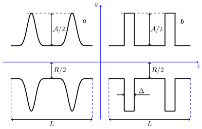
Figure 1: Sketch of the periodic structures considered in this work. (a) Smooth channel (Sm); (b) Sharp channel (Sh). We identify $H$–regions (humps) of the channel such that $R/2<|y|\leq\omega(x)$ and the $S$–region (shaft) $|y|\leq R/2$. Diffusion regimes inside these channels depend on the ratio $Q=\mathcal{A}/R$ controlling the importance of the $H$ regions over the $S$ region. When not specified, we consider channels with fixed shaft parameters $L=10$, $R=4$, whereas, the size of the $H$–regions will be changed to obtain stronger or weaker lateral particle trapping.

Let us assume that the channel is parallel to the $x$–axis and its cross section $\sigma(x)$ varies periodically on the longitudinal direction. It is convenient to introduce the marginal density [21, 22, 4] $\mathscr{G}(x,t)$, defined by

$$\mathscr{G}(x,t)=\int_{-\omega(x)}^{+\omega(x)}\!\!\!\!\!dy\;\mathscr{P}(x,y,t)$$ (4)

where we considered a symmetric channel along its longitudinal axis described by the boundary profile $y=\pm\omega(x)$, thereof the cross section is $\sigma(x)=2\omega(x)$.

Rather general procedures of the multiscale technique suggest the validity at large time of a parabolic equation governing the diffusion along the $x$–direction [13, 23, 24] given by

$$\frac{\partial\mathscr{G}(x,t)}{\partial t}=\frac{\partial}{\partial x}\left\{\sigma(x)D(x)\frac{\partial}{\partial x}\left[\frac{\mathscr{G}(x,t)}{\sigma(x)}\right]\right\}\;.$$ (5)

Jacobs in his book on diffusive processes [13] used the drastic approximation

$$D_{\mathrm{FJ}}(x)=D_{0}\;,$$ (6)

assuming that in narrow-enough channels the distribution of particles in any cross section becomes swiftly uniform (local equilibrium).

Several authors [23, 25] argued that deviations from transversal homogeneity are not negligible and need to be taken into account by a diffusion coefficient $D=D(x)$ varying with the longitudinal coordinate. The specific expression of $D(x)$ depends on the channel boundaries and guessing the appropriate functional form for given geometry is a central task of this kind of problems. Zwanzig for example [23] derived a perturbative expression for $D(x)$ in a two dimensional channel,

$$D_{\mathrm{Zw}}(x)=D_{0}\left[1+\frac{1}{12}\left(\frac{d\sigma}{dx}\right)^{2}\right]^{-1}$$ (7)

which holds under the hypothesis $|\sigma^{\prime}(x)|\ll 1$.

Instead, Reguera and Rubí (RR) using a heuristic argument [1] proposed the expression

$$D_{\mathrm{RR}}(x)=D_{0}\left[1+\frac{1}{4}\left(\frac{d\sigma}{dx}\right)^{2}\right]^{-1/3}\;.$$ (8)

Finally, Kalinay and Percus (KP) performing an elegant perturbative treatment in order to expand $D(x)$ in $\sigma(x)$ and its derivatives [21, 26, 24, 27] obtained, for a 2D channel, to the lowest order the expression

$$D_{\mathrm{KP}}(x)=D_{0}\frac{\arctan{\left(\dfrac{1}{2}\dfrac{d\sigma(x)}{dx}\right)}}{\dfrac{1}{2}\dfrac{d\sigma(x)}{dx}}\,.$$ (9)

It is easily to verify by a series expansion in $|\sigma^{\prime}(x)|$ that, to the lowest order, all the functional forms coincide $D_{\mathrm{KP}}(x)=D_{\mathrm{RR}}(x)=D_{\mathrm{Zw}}(x)\approx D_{0}(1-\sigma^{\prime}(x)^{2}/12)$.

Once an explicit expression of $D(x)$ has been established, Eq. (5) provides the values of $D_{\mathrm{eff}}$ through the Lifson–Jackson (LJ) formula [28]

$$D_{\mathrm{eff}}=\frac{1}{\langle\sigma(x)\rangle\left\langle\displaystyle\frac{1}{D(x)\sigma(x)}\right\rangle}$$ (10)

where the angular brackets denote the spatial average over a period $L$ of the channel

$$\langle f(x)\rangle=\frac{1}{L}\int_{x_{0}}^{x_{0}+L}\!\!\!\!\!\!\!dx\;f(x),$$

with $f(x)=f(x+L)$.

Once the asymptotic diffusion process has been reduced to the effective one-dimensional PDE (5), the problem can be also recast into the corresponding one-dimensional Langevin equation

$$\frac{dx}{dt}=-\frac{dV(x)}{dx}+\sqrt{2D(x)}\xi(t)$$

with an effective potential

$$V(x)=-k_{B}T\ln{\sigma(x)}$$

where $V(x)$ is a periodic function depending on $\sigma(x)$ and represents an entropic potential [16].

The perturbative approach of Refs. [23, 27, 29] fails to describe the most interesting cases where $\mathcal{A}\gtrsim R,L$ or becomes particularly involved [30] when dealing with not differentiable boundaries of the channel (see Fig. 1).

II Asymptotic Diffusion

Let us introduce a simple argument to derive an approximation to the effective coefficient $D_{\mathrm{eff}}$ of the longitudinal diffusion.

Of course, the trapping mechanism due to the humps implies that $D_{\mathrm{eff}}<D_{0}$. With reference to Fig. 1, we shall dub “Humps” ($H$) and “Shaft” ($S$) the sets of the channel such that

$$H = \{(x,y)\in\mathbb{R}^{2}~{}|~{}R/2<|y|\leq\omega(x)\}$$

$$S = \{(x,y)\in\mathbb{R}^{2}~{}|~{}|y|\leq R/2\}.$$ (11)

Within the $H$ region the particles spend a certain amount of time before coming back to the $S$ region where they contribute to the transport along the $x$–direction.

We consider two types of structures sketched in Fig. 1. The first (Fig. 1a) is defined by the smooth boundary

$$\omega_{\mathrm{Sm}}(x)=\dfrac{R+s(\gamma)\mathcal{A}}{2}+\dfrac{\mathcal{A}}{2}\sin^{\gamma}\left(\dfrac{2\pi x}{L}\right)$$ (12)

where $\gamma$ is an integer tuning the shape of the humps: the larger $\gamma$, the sharper the sinusoidal humps and $s(\gamma=2n)=0$, $s(\gamma=2n+1)=1$. The extra term, $s(\gamma)\mathcal{A}/2$, when $\gamma$ turns from even to odd values is necessary to avoid the upper- and lower-boundary overlap and to keep the $S$-region width fixed to $R$. Analogously, the period of the “even” and “odd” profiles changes from $L/2$ to $L$. Hereafter, this channel is referred to as the Smooth channel (Sm).

The other structure that we name Sharp channel (Sh), Fig. 1b, is characterized by the step-like profile

$$\omega_{\mathrm{Sh}}(x)=\begin{cases}\dfrac{R+\mathcal{A}}{2}&\dfrac{L}{4}-\dfrac{\Delta}{2}\leq|x|<\dfrac{L}{4}+\dfrac{\Delta}{2}\vspace{0.8em}\\ \dfrac{R}{2}&\mbox{elsewhere}\end{cases}$$ (13)

The period of this channel is $L/2$. More complicated boundaries will be taken into account in the following. Unless otherwise stated, throughout the text and in all simulations, we consider channels with fixed shaft parameters: $L=10$, $R=4$, whereas, the parameters controlling the size and the shape of the $H$-regions, such as $\mathcal{A}$, $\gamma$ and $\Delta$, will be tuned to obtain different degrees of dead-end trapping.

We introduce a phenomenological Markov process to estimate $D_{\mathrm{eff}}$. Let us observe that in the long time limit, the motion along the transverse direction becomes stationary. Thus the probabilities $P_{H}(t)$ and $P_{S}(t)=1-P_{H}(t)$ to be in the $H$ and $S$ regions respectively become constant at large times,

$$\lim_{t\to\infty}P_{S}(t)=P^{eq}_{S}=\frac{\mu(S)}{\mu(H)+\mu(S)},$$ (14)

where $\mu(S)$ and $\mu(H)$ are the areas (measure) of the $S$ and $H$ regions respectively within a single period of the channel. Since we are interested only in the longitudinal transport process, we can approximate the particle motion as a random walk on a 1D “lattice” where the walkers can either jump to the left or to the right with probability $\mu(S)$ or they can sit on the same site with probability $\mu(H)$. In this coarse–grained representation which mimics the longitudinal diffusion process, $D_{\mathrm{eff}}$ can be expressed in the form

$$D_{\mathrm{eff}}=D_{0}P_{S}^{eq}\;.$$ (15)

Notice that the result coincides with the one proposed in Refs. [31, 32].

Equations (14) and (15) when applied to the Sm-channel (12) provide the result

$$\frac{D_{\mathrm{eff}}}{D_{0}}=\begin{cases}\dfrac{R}{R+\dfrac{1}{\pi}B\left(\dfrac{1}{2},\dfrac{\gamma+1}{2}\right)\mathcal{A}}&\mbox{if~{}}\gamma=2n\vspace{0.5em}\\ \dfrac{R}{R+\mathcal{A}}&\mbox{if~{}}\gamma=2n+1\end{cases}$$ (16)

where $B(a,b)=\Gamma(a)\Gamma(b)/\Gamma(a+b)$ is the Euler’s $\beta$ function.

The dependence of $D_{\mathrm{eff}}$ on even $\gamma$’s at $R$ and $\mathcal{A}$ fixed is determined by the behavior of the function $B[1/2,(\gamma+1)/2]$, which monotonically decreases with $\gamma$ and asymptotically scales like $B\sim\sqrt{2/(\pi\gamma)}$. This implies that $D_{\mathrm{eff}}$ approaches $D_{0}$ at large even $\gamma$s, which is not a surprising situation if one considers that a very large $\gamma$ determines inaccessible narrow Humps in the profile (12), consequently, the particles are constrained to perform a free diffusion along the Shaft region.

For odd $\gamma$, the area cancellation in $\mu(H)$ yields a result that is independent of the Hump’s shape and the $\gamma$–value as well. This peculiarity makes the applicability of the areas’ formula critical to “odd” channels, as we discuss later.

For the Sharp channel (13), we obtain

$$\mu(S)=RL,\qquad\mu(H)=2\mathcal{A}\Delta\;,$$

and the effective coefficient reads

$$\frac{D_{\mathrm{eff}}}{D_{0}}=\frac{RL}{RL+2\mathcal{A}\Delta}.$$ (17)

Equations (16) and (17) can be recast in a common form highlighting the relevant dependence on the ratio $Q=\mathcal{A}/R$,

$$\frac{D_{\mathrm{eff}}}{D_{0}}=\dfrac{1}{1+g_{H}Q};$$ (18)

where $g_{H}$ is a coefficient depending on the finer details of the hump regions; in particular, $g_{H}=1$ ($\gamma$ odd), $g_{H}=B[1/2,(\gamma+1)/2]/\pi$ ($\gamma$ even) for a Sm-channel, while $g_{H}=2\Delta/L$ in a Sh-channel.

It is interesting to remark that Eq.(17) is amenable to an alternative derivation suggested by the general multiscale techniques [33] where the concept of an effective diffusion equation along the channel centerline naturally arises, namely

$$\partial_{t}P(x,t)=\partial_{x}\{\tilde{D}(x)\partial_{x}P(x,t)\}$$ (19)

note that now $\tilde{D}(x)$ embodies all the inhomogeneities of the problem and thus does not coincide with $D(x)$ of Eq. (5). Equations (5) and (19) need not be related in a direct mathematical way as they provide only an equivalent mesoscopic representation of the same asymptotic process: the large time diffusive behavior when the transversal homogenization has been achieved.

The above formulation has the advantage that the result (17) can be still recovered through (10) providing one assumes a local diffusion coefficient such that

$$\tilde{D}(x)=\begin{cases}D_{0}\dfrac{R}{\mathcal{A}+R}&\dfrac{L}{4}-\dfrac{\Delta}{2}\leq|x|<\dfrac{L}{4}+\dfrac{\Delta}{2}\vspace{0.8em}\\ D_{0}&\mbox{elsewhere}\end{cases}.$$ (20)

Such a proposal can be rationalized as follows. A particle can fully contribute to the diffusion only when its $y$ coordinate lies in the $S$-region. Accordingly, if the particle is in the $S$-region, its diffusion occurs with a free coefficient $D_{0}$, whereas in the $H$-region the diffusion coefficient is depressed by a factor $R/(\mathcal{A}+R)$. Now from expression (20) we can compute the effective diffusion coefficient as

$$D_{\mathrm{eff}}=\dfrac{1}{\left\langle\dfrac{1}{\tilde{D}(x)}\right\rangle}\,.$$

This approach, in a philosophy similar to the homogenization technique, amounts to considering a flat channel while shifting its inhomogeneity to the diffusion coefficient and it has the advantage to be also applicable to not differentiable boundary profiles.

In order to test the quality of the approximation (18), we performed numerical simulations by integrating the Langevin equation (1) with $V(\mathbf{r})=0$. The no-flux condition has been implemented both via a simple rejection algorithm and via an elastic-reflection method in the collision of a particle against the wall. The results were independent of the method and we opted for the rejection method which is faster and of easier implementation. We simulated $N=7\times 10^{4}$ independent particle trajectories via a standard Euler’s scheme with $D_{0}=1$ and a time step $\Delta t=0.005\tau$, where $\tau=R^{2}/2D_{0}$ and $R$ is the fixed cross section of the shaft region (see Fig. 1). Hence, for each time step, the mean step length $\Delta\ell=\sqrt{2D_{0}\Delta t}\simeq 0.07R$, turns out to be reasonably smaller than the typical geometrical length of the channel but large enough to avoid excessively long simulation runs.

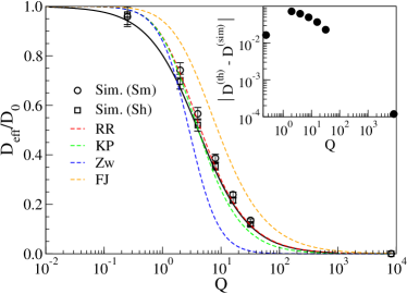
Figure 2: Plot of Eq. (18) vs $Q=\mathcal{A}/R$ (black line) together with the simulated $D_{\mathrm{eff}}$ data obtained by the slope of $\langle\Delta x^{2}(t)\rangle$ in the linear regime. Symbols correspond to values $Q=2^{-2},2^{1},2^{3},\cdots 2^{13}$; circles refer to the Sm-channel with $L=10,R=4,\gamma=10$, while squares refer to the Sh-channel with $L=10,R=4,\Delta=1.23$. Since the channels are equivalent (same area), the data from both structures are supposed to collapse onto each other. The percentage error is within 4%; the inset instead shows the deviation $|D_{\mathrm{eff}}(\mathrm{th})-D_{\mathrm{eff}}(\mathrm{sim})|$ of the black line from the open circles in the main panel. For a further comparison, we report the $D_{\mathrm{eff}}$ of the Sm-channel computed by Eq.(10) using the local diffusion coefficients mentioned in the text: $D_{RR}(x)$ (red), $D_{KP}(x)$ (green), $D_{Zw}(x)$ (blue), and $D_{FJ}(x)$ (orange).

The numerical results are shown in Fig. 2, where formula (18) is compared to the simulation data obtained from the asymptotic behaviour of the longitudinal MSD in the Sm- and Sh-channels at different values of $Q=\mathcal{A}/R$. We have chosen $L=10$ and $R=4$ for both structures and set $\gamma=10$ for the smooth boundary and $\Delta=B(1/2,11/2)L/\pi=1.23$ for the sharp boundary in order to have a unique $g_{H}$ in Eq. (18), which means equivalent channels (i.e. with the same area). The dashed lines in Fig. 2 show the values of $D_{\mathrm{eff}}$ of the Sm-channel obtained by the LJ-formula (10) via a numerical evaluation of the integrals for various expressions of the local diffusion coefficient.

The LJ formula cannot be applied to the Sh-channel, as $\omega_{\mathrm{Sh}}(x)$ is not differentiable everywhere. In this case, another approximation which can be very useful is based on the boundary homogenization [34, 35, 36]. The method was applied by Berezhkovskii and co–workers [22] to the calculation of $D_{\mathrm{eff}}$ for the Sh-channel, however their result is valid under the restriction $2\Delta\geq 2\mathcal{A}+R$ which is not assumed here.

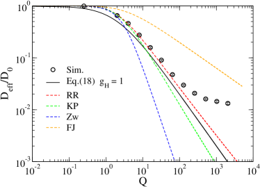
Figure 3: Comparison between simulated data of $D_{\mathrm{eff}}$ (circles) and the theoretical prediction (18) (black line) for the unbiased diffusion in a Sm–channel, with $\gamma=1$ and the other parameters as in Fig. 2. The percentage error on simulation data is within 4%. The accuracy of Eq.(18) worsens at increasing $Q=\mathcal{A}/R$. Dashed lines represents the predictions of $D_{\mathrm{eff}}$ yielded by the generalized FJ approach involving the same $D(x)$ expressions of Fig. 2.

The formula of geometrical areas (15) reveals some inaccuracy in predicting the $D_{\mathrm{eff}}$ behaviour for the Sm-channel with odd $\gamma$, indeed, the case $\gamma=1$ reported in Fig. 3 shows that the agreement between Eq. (18) (solid line) and the simulation data (symbols) dramatically worsens in the range of large $Q=\mathcal{A}/R$.

This discrepancy can be justified by observing that Eq. (18) remains a reliable approximation of $D_{\mathrm{eff}}$ as long as the channel partitioning in $H$ and $S$ regions is not ambiguous. Actually, the $S$ and $H$ distinction is not always physically meaningful, just like in the case of the Sm-channel with odd $\gamma$. The crucial difference between odd and even $\gamma$ is apparent in Fig. 4.

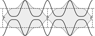
Figure 4: Sketch of a Sm-channel with even (solid) and odd (shaded) $\gamma$. Notice the concavity change of the profile when $\gamma$ turns from even to odd. For $\gamma$ odd, the $H$-region of the channel becomes predominant whereas the $S$-domain remains ill-identified as it is restricted to point-like regions marked by the letter $P$. In this case, the structure becomes equivalent to a septate channel [37] of section $R+\mathcal{A}$ (dashed lines) for which Eq. (15) fails.

When $\gamma$ is odd, the $S$-domain turns out to be ill defined as it shrinks to point-like regions (marked by $P$s in the figure). Conversely, the $H$-regions are so large that produce a negligible trapping mechanism. The resulting structure is virtually equivalent to a “septate channel” [37] of section $R+\mathcal{A}$, namely, an array of compartments connected by holes in the separating walls (dashes shape in Fig. 4). As it discussed in Ref. [5], the derivation of $D_{\mathrm{eff}}$ in septates requires a different approach from the one leading to Eq.(18).

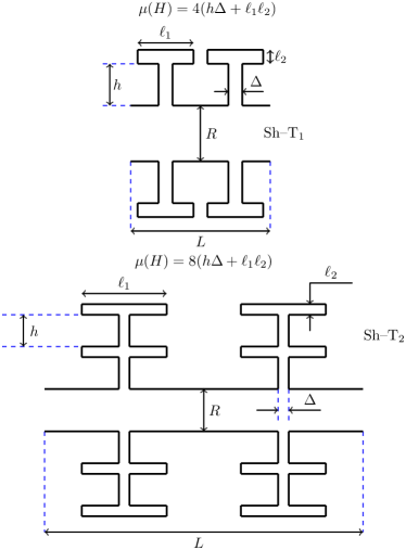
Figure 5: Examples of sharp channels Sh-T₁ and Sh-T₂ with a boundary profile $\omega(x)$ which is a multivalued function of the longitudinal position; in that case the generalized FJ approximation cannot be used. In both structures, the parameters, $h,\Delta,\ell_{1},\ell_{2}$ are tuned such that $\mu(H)$ coincides with the Hump area of the boundaries used to generate Fig. 2.

Apart from the peculiarity of the septates, Eq.(15) is rather general as it works well in a variety of geometries. For instance, it is able to predict the $D_{\mathrm{eff}}$ associated with the complex channels Sh-T₁ and Sh-T₂ sketched in Fig. 5. This can be appreciated from the results in Fig. 6 showing a comparison of $D_{\mathrm{eff}}$ from Brownian simulations in Sh-T₁ and Sh-T₂ (symbols) to its theoretical prediction based on Eq.(15) (dashed line). The different sets of data refer to structures with different profiles but the same hump area $\mu(H)$. The perfect collapse of the different data onto the same theoretical curve confirms the great accuracy of Eq.(18).

This example clearly indicates that, when the $S$-$H$ partition of a channel is not ambiguous and the $H$-regions perform a sufficient trapping action on the particles, the area’s formula (18) is able to catch the right dependence of $D_{\mathrm{eff}}$ on the channel geometry, despite the complexity of the section.

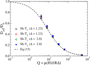
Figure 6: Plot of $D_{\mathrm{eff}}/D_{0}$, theory (dashed line) and simulation data (symbols) vs $Q=\mu(H)/(R\Delta)$ referred to the structures Sh-T₁ and Sh-T₁ drawn in Fig. 5. We considered channels with two $\Delta$ values and tuned the other parameters ($h,\ell_{1},\ell_{2}$) to maintain the same Hump area in both structures. For this reason different data sets collapse onto each other. The agreement between theory and simulation results is convincing despite the geometric complexity of the channels. The percentage error on data is about 4% leaving the bars well below the symbol size.

III Pre–asymptotic diffusion

Generally, the study of pre–asymptotic or transient regimes is important to gain information about a possible trapping mechanism and memory effects in a dynamical processes [38, 39]. In the specific case of corrugated channel, the temporary trapping of particles within the $H$ regions can induce a transient behaviour which generally depends on the system preparation and it could be characterized by nonlinear growth of the mean square displacement [40, 31]. There exists a crossover time $\tau_{\parallel}$ separating the pre–asymptotic and the asymptotic motion that is affected by the initial particle distribution in the channel, $\tau_{\parallel}=\tau_{\parallel}(\mathbf{r}_{0})$, $\mathbf{r}_{0}$ being a shorthand notation for the initial position of all the particles. We considered three types of initial conditions in the channel of Fig. 1b: i) a uniform distribution of particles in the $S$-region of a single unitary cell, $\mathbf{r}_{0}\in S$, ii) the particles uniformly distributed in one period of the $H$-region, $\mathbf{r}_{0}\in H$, and finally iii) a uniform distribution over the whole unit cell $\mathbf{r}_{0}\in S\cup H$.

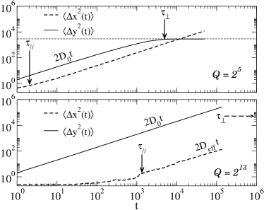
Figure 7: Comparison between the relaxation of longitudinal $\langle\Delta x(t)^{2}\rangle$ and transversal $\langle\Delta y^{2}(t)\rangle$ diffusion for the same channel of Fig. 8 with two different values of $Q=2^{5}$ and $Q=2^{13}$. The system is prepared uniform over $S\cup H$, but the large $Q$ values prevents the fast lateral homogenization. In the case $Q=2^{5}$, the homogenization takes place at times $\tau_{\parallel}<\tau_{\perp}$, while for $Q=2^{13}$ the homogenization becomes particularly slow ($\tau_{\perp}\simeq 3^{9}$) and it delays the onset of the standard diffusion along the $x$-axis, $\tau_{\perp}\simeq 10^{3}$. Moreover as long as $t<\tau_{\perp}$, the lateral diffusion satisfies $\langle\Delta y^{2}(t)\rangle=2D_{0}t$, supporting the derivation of Eq.(24) and Eq.(25). The horizontal dashed line marks the value $2D_{0}\tau_{\perp}(S\cup H)=R^{2}(1+Q)^{2}/6$ obtained from the last line of Eq.(21).

The “local equilibrium” assumption [23, 4] requires that the typical relaxation time $\tau_{\perp}$ after which the particle distribution becomes uniform in each cross section is much smaller than $\tau_{\parallel}\gg\tau_{\perp}$ where $\tau_{\perp}$ is estimated assuming a flat final $y$ distribution on each section $[-\omega(x),\omega(x)]$,

$$\tau_{\perp}=\frac{\langle[y(\infty)-y(0)]^{2}\rangle}{2D_{0}}=\frac{\sup_{x}\{\omega^{2}(x)\}}{6D_{0}}+\frac{\langle y^{2}(0)\rangle}{2D_{0}},$$

the angular brackets indicate the double average over the final and initial distributions. In the first term, $\sup_{x}\{\omega^{2}(x)\}=(R+\mathcal{A})^{2}/4$ for both Sm and Sh channels, the value $\langle y^{2}(0)\rangle$ depends on the starting particle distribution. In particular, for the distributions i)–iii) just mentioned we have,

$$\tau_{\perp}(\mathbf{r}_{0})=\tau_{R}\begin{cases}(1+Q)^{2}+1\qquad\mathbf{r}_{0}\in S\vspace{0.5em}\\ (1+Q)^{2}+\dfrac{(1+Q)^{3}-1}{Q}\quad\mathbf{r}_{0}\in H\vspace{0.5em}\\ 2(1+Q)^{2}\qquad\mathbf{r}_{0}\in S\cup H.\end{cases}$$ (21)

with $\tau_{R}=R^{2}/(12D_{0})$. Taking $Q$ sufficiently large, $\tau_{\perp}$ can be made so arbitrarily long that the transversal homogenization becomes considerably slow and the assumption of a sharp scale separation $\tau_{\perp}\ll\tau_{\parallel}$ certainly fails. This very slow transversal homogenization induces a delay on the onset of the standard longitudinal diffusion that can be observed in Fig. 7, where we plot the relaxation of longitudinal and transversal MSD in a sharp channel for a moderate $Q=2^{7}$ and large $Q=2^{15}$. In both cases, the vertical homogenization established later than the occurrence of the normal diffusion along the channel axis. However in the second case, the onset of a longitudinal standard regime is strongly retarded by the lack of lateral homogenization.

Therefore, we shall focus on the pre–asymptotic diffusion in channels with large enough $Q$, where, more likely, the local equilibrium condition is violated. Figure 8 shows the log–log plot of the longitudinal MSD for the three initial distributions i)–iii) defined above in the Sh-channel (13) with $Q=2^{5}$, the inset reports the same data for $Q=2^{2}$. The plot emphasizes the transient nonlinear behaviour of MSD and the dependence of the dynamics on the initial condition.

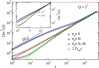
Figure 8: Log–log plot of $\langle\Delta x^{2}(t)\rangle$ in a Sh-channel with $Q=2^{5}$ as a function of the time for the system starting from three initial conditions: $\mathbf{r}_{0}\in H$ (squares), $\mathbf{r}_{0}\in H\cup S$ (triangles), $\mathbf{r}_{0}\in S$ (circles). Symbols refer to the simulation data whereas the dashed lines represent their fit by Eq. (25) upon tuning the free parameter $\tau_{0}$. Parameters $R,L,\Delta$ are as in Fig. 2. The inset shows the same results for $Q=2^{2}$.

The different short-time behaviour of the three sets of data can be explained as follows. The particles initialized with $\mathbf{r}_{0}\in S$ perform a stage of free diffusion (coefficient $D_{0}=1$) until they are trapped into the Humps, accordingly their MSD initially grows like $\langle\Delta x^{2}(t)\rangle\simeq 2D_{0}t$ (circles). The opposite case corresponds to all the particles initialized in $\mathbf{r}_{0}\in H$. Their MSD remains stacked to a small value (squares) due to the trapping of Humps until enough particles begin to escape. Obviously, the MSD of particles uniformly initialized in $\mathbf{r}_{0}\in H\cup S$ exhibits a short-time behaviour that is intermediate between the two opposite cases.

The global behaviour of $\langle\Delta x^{2}(t)\rangle$ as a function of the elapsed time can be qualitatively understood by the following argument. The growth $\langle\Delta x^{2}(t)\rangle$ can be related to the occupation probability $P_{S}(t)$ of the $S$ region at time $t$ [31]

$$\langle\Delta x(t)^{2}\rangle=2D_{0}\int_{0}^{t}\!du\;P_{S}(u)$$ (22)

In the Appendix A, we show how Eq. (22), which generalizes Eq. (15) to transient diffusion, can be justified by exploiting some intuitive similarities between the diffusion in corrugated channels and the unbiased random walks on a comb lattice with finite sidebranches. Equation (22) is, of course, meaningful only if the $S$ and $H$ regions can be unambiguously identified. If so, we can define a coarse–grained description of the process in terms of a two-state kinetic model, where the states $S$ and $H$ have probabilities $P_{S}(t)$ and $P_{H}(t)=1-P_{S}(t)$, respectively. Let $k_{\mathrm{S}}(t)$ and $k_{\mathrm{H}}(t)$ be the transition rates from $S$ to $H$ and from $H$ to $S$ respectively, then the rate equation for $P_{S}(t)$ reads

$$\frac{dP_{S}(t)}{dt}=-k_{\mathrm{S}}(t)P_{S}(t)+k_{\mathrm{H}}(t)[1-P_{S}(t)].$$ (23)

We considered the limiting case of large $\mathcal{A}$, in which the strong trapping mechanism delays the longitudinal equilibration (homogenization), see Fig. 7. Accordingly, for $t\ll\tau_{\perp}$ the diffusion in the $y$ direction is still an ongoing process, $\langle\Delta y^{2}(t)\rangle\sim t$. In a first approximation, we can argue that $k_{S}(t)$ and $k_{H}(t)$ are proportional to the typical spreading velocity of the transversal diffusion, thus,

$$k_{\mathrm{S}}(t)\sim a/\sqrt{t},\qquad k_{\mathrm{H}}(t)\sim b/\sqrt{t};$$

where $a$ and $b$ are dimensional constants to be determined by phenomenological considerations. Substituting the rates into Eq. (23), we get the solution

$$P_{S}(t)=P_{S}(0)\mathrm{e}^{-2(a+b)\sqrt{t}}+\frac{b}{a+b}\left(1-\mathrm{e}^{-2(a+b)\sqrt{t}}\;\right).$$

Now the parameters $a$ and $b$ can be expressed in terms of meaningful physical quantities by setting: $2(a+b)=1/\sqrt{\tau_{0}}$, where $\tau_{0}$ is a free time scale to be adjusted, and $b/(a+b)=D_{\mathrm{eff}}/D_{0}$, which comes from the equilibrium condition $P_{S}(t)\to P_{S}^{eq}$. After simple algebra we obtain $a=(1-D_{\mathrm{eff}}/D_{0})/\sqrt{4\tau_{0}}$ and $b=D_{\mathrm{eff}}/(D_{0}\sqrt{4\tau_{0}})$.

Thus, the final expression for $P_{S}(t)$ reads

$$P_{S}(t)=P_{S}(0)\mathrm{e}^{-\sqrt{t/\tau_{0}}}+\frac{D_{\mathrm{eff}}}{D_{0}}\left(1-\mathrm{e}^{-\sqrt{t/\tau_{0}}}\;\right)$$ (24)

and according to Eq.(22), we derive the MSD

$$\langle\Delta x(t)^{2}\rangle=2D_{\mathrm{eff}}t+C\left\{1-\mathrm{e}^{-\sqrt{t/\tau_{0}}}\left(\sqrt{t/\tau_{0}}+1\right)\right\},$$ (25)

with $C=4D_{0}\tau_{0}[P_{S}(0)-D_{\mathrm{eff}}/D_{0}]$. The phenomenological expression (25) can be used to fit the MSD data of Fig. 8 by adjusting the $\tau_{0}$ value. The blue dashed line represents Eq.(25) with the initial condition $P_{S}(0)=1$, corresponding to all the particles in the $S$ region. Since $C$ is positive, the second term in Eq.(25) contributes positively to the MSD and the convergence to the asymptotic behaviour $2D_{\mathrm{eff}}t$ is from above. When the particles start in the $H$ region, $P_{S}(0)=0$, Eq. (25) corresponds to the dashed green line, in this case $C<0$ and the convergence to the slope $2D_{\mathrm{eff}}t$ is from below. Finally, if the particles are initialized with a uniform distribution so that $P_{S}(0)=P_{S}^{eq}=D_{\mathrm{eff}}/D_{0}$, the constant $C$ in Eq. (25) vanishes and the system achieves soon the expected standard diffusive behaviour (red dashed line). The agreement between simulation data and the fitting curves is satisfactory considering that Eq. (25) has only one free parameter and that its derivation is based just on reasonable assumptions.

The regime with $\mathcal{A}$ comparable with all the other geometrical sizes can be captured by a generalization of Eq. (24) where the square-root dependence $\sqrt{t/\tau_{0}}$ is replaced by the power law $(t/\tau_{0})^{\nu}$, with $\nu$ being an additional fitting parameter. The inset of Fig. 8 shows the example with $\mathcal{A}=2^{3}$, for which we found $\tau_{0}\approx 18$ and $\nu\approx 0.7$.

IV Einstein’s Fluctuation Dissipation Relation.

We discuss the transport problem in the presence of small external longitudinal field $\mathbf{F}=f\hat{\mathbf{x}}$, i.e., $fL/(2k_{\mathrm{B}}T)\ll 1$. In particular, we are interested in possible generalization of the Einstein’s (FDR) to regimes where the approach to the “transversal equilibrium” is so slow that a robust transient behaviour of non standard longitudinal diffusion can be observed.

In the linear response regime, the asymptotic mean drift induced by the field $f$ is

$$\langle\Delta x(t)\rangle_{f}=\mu_{\mathrm{eff}}ft,$$

where $\mu_{\mathrm{eff}}$ is the effective mobility, and since the asymptotic MSD for $f=0$ is given by

$$\langle\Delta x^{2}(t)\rangle_{0}=2D_{\mathrm{eff}}t,$$

the ratio

$$\frac{\langle\Delta x(t)\rangle_{f}}{\langle\Delta x^{2}(t)\rangle_{0}}=\frac{\mu_{\mathrm{eff}}}{D_{\mathrm{eff}}}\frac{f}{2}=\mbox{const}.$$ (26)

remains constant in time, assuming Einstein’s FDR $D_{\mathrm{eff}}=k_{B}T\mu_{\mathrm{eff}}$, the const is fixed to $f/(2k_{B}T)$. Here we work in units such that $k_{B}T=1$.

Previous studies [2, 5, 17, 32] mainly focused on the validity of FDR in the asymptotic regime and worked out analytical expressions for the linear and nonlinear mobility $\mu_{\mathrm{eff}}$, here we test Eq.(26) when the diffusion is not yet asymptotic. This analysis can be guided by the structural similarity that channels with $\mathcal{A}/R\gg 1$ share with the comb lattice with long but finite sidebranches (Fig. 11 of the Appendix A): the backbone and teeth of the comb play the role of the $S$ and $H$ regions of the channel. This similarity reflects also on the transport properties, indeed Fig. 9 shows that in the limit $Q=\mathcal{A}/R\gg 1$ the diffusion along the channel becomes anomalous $\langle\Delta x^{2}(t)\rangle_{0}\sim t^{2\nu}$ with the same exponent $\nu=1/4$ of the random walk on a comb [41, 42, 43]. This scenario is consistent with the behavior $D_{\mathrm{eff}}\sim 1/\mathcal{A}$ at large $\mathcal{A}$ [see Eqs.(16) and (17)], which is a physical consequence of the trapping action exerted on particles by very long humps. The Appendix A shows that on a comb lattice such a regime, though anomalous, does satisfy the FDR at any time due to an accidental but exact cancellation in the ratio (26). We stress that in the comb lattice, Eq.(26) is exact not only at any times but also for any initial particle distribution. In analogy, as long as the random walk on the comb constitutes a good representation of the continuum process, we expect FDR to maintain a certain validity for the diffusion in channels even in non-asymptotic regimes and regardless of the initial particle distribution, provided it is generic enough.

Figure 9: Log–log plot of the MSD versus the elapsed time for the channel sketched in Fig. 1(b) with increasing values of $\mathcal{A}$. For $\mathcal{A}/R=2^{8}$, the diffusion is anomalous $\langle\Delta x^{2}(t)\rangle_{0}\sim t^{1/2}$ with the same exponent of the random walk on a comb, $2\nu=1/2$, supporting the view that the structure in Fig. 1(b) virtually behaves as a comb at enough large $\mathcal{A}$.

To verify this, we performed numerical simulations of diffusion driven by different external fields and in channels with increasing $\mathcal{A}/R$. The plot of $\langle\Delta x(t)\rangle_{f}$ versus $\langle\Delta x^{2}(t)\rangle_{0}$ for different values of $Q=\mathcal{A}/R$ is shown in Fig 10, where symbols are the numerical data and dashed straight lines represent the expected behaviour as predicted by taking the logarithm of both members of Eq.(32). The perfect alignment of data along the lines confirms the exact proportionality between the MSD and the mean drift according to Eq.(26).

We note that in systems governed by a one-dimensional Fokker-Planck equation, the Einstein’s relation holds exactly at any time if the initial condition coincides with the invariant probability distribution [44]. The same applies also to the fractional Fokker-Planck equation [45] describing anomalous diffusion.

In conclusion, although both $\langle\Delta x(t)\rangle_{f}$ and $\langle\Delta x^{2}(t)\rangle_{0}$ depend on the channel shape and on the initial system preparation, their ratio remains constant in time in any explored regime, generalizing “de facto” the Einstein relation to the pre-asymptotic dynamics.

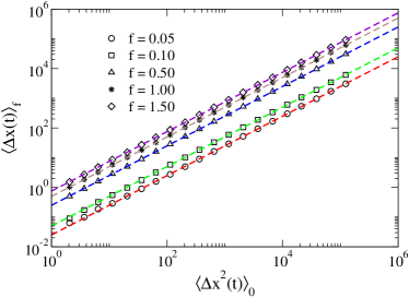
Figure 10: Check of the FDR for the diffusion in Sh-channels-(13). Log–log plot of $\langle\Delta x(t)\rangle_{f}$ vs $\langle\Delta x^{2}(t)\rangle_{0}$, symbols are the simulation results, and dashed lines represent the theoretical expectation (26), which is verified regardless of the $\mathcal{A}$ value and turns out to be independent of the initial particle distribution within the channel. The FDR is exactly satisfied also in smooth channels (not shown).

V Conclusions

This paper analyzed the diffusion in channels with nonuniform sections in conditions well beyond the range of applicability of the FJ approximation, which properly works only for small deviations from the homogeneous channel. We performed Brownian dynamics simulations in different geometries considering even channels with steep variations of the boundaries and computed numerically the effective diffusion coefficient $D_{\mathrm{eff}}$ from the asymptotic behavior of the mean square displacement (MSD). We compared the numerical results to the predictions from the various corrections to the FJ theory, suggested in the literature, that make use of a local diffusion coefficient within the Lifson–Jackson formula. We then focused on channel profiles which are not differentiable (sharp channels) for which the FJ approximation and its corrections turns out to be of difficult application. In these cases, there exists a semi-heuristic approach based on the large-time limit of formula (22) which allows $D_{\mathrm{eff}}$ to be expressed in terms of the geometrical weight of region $H$, where particles contribute to the longitudinal diffusion and dead-end region $S$, where particles are temporarily trapped. We tested numerically the applicability of Eq. (22) to different channel geometries and we found that it works fine only when the partition of the channel into $S$ and $H$ regions is unambiguous. In other words, the trapping mechanism of the dead-ends should be strong enough to introduce a scale separation between moving and trapped dynamics. When this scale separation does not occur the theoretical prediction deviates from the numerical data.

In addition, we characterized the transient regime of the diffusive transport by measuring nonlinear behaviour of the MSD before it attains the linear growth. These transients for specific channel profiles can be made arbitrarily long and robust by acting on the channel geometry. Also in this case we analyzed the data according to formula (22) obtaining a satisfactory description of the MSD growth in terms of the solution of phenomenological rate equation for the probability to occupy the $S$-region. We proved that Einstein’s relation can be remarkably established between the mean drift of the biased diffusion in a small field along the channel axis and the MSD of the unbiased diffusion, in both asymptotic and pre-asymptotic regimes.

Appendix A

This appendix shows the derivation of formula (22) and the response by exploiting the analogy between the diffusion in a channel geometry with very large $\mathcal{A}$ and the random walk on the comb lattice with finite length sidebranches (Fig. 11).

The comb lattice is composed of periodic arrangements of transversal teeth of length $L$, attached to the backbone of the structure, which represents the transport direction as shown in Fig. 11. For simplicity, we consider here the case of unitary spaced teeth. The sidebranches in comb lattice mimics, to some extent, the trapping mechanism of “Hump” regions ($H$) of the channel. The backbone corresponds to the region “$S$” where diffusion is not hindered and the drift is efficient.

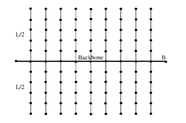
Figure 11: Sketch of the regular comb lattice used for its analogy to channels with narrow and long hump regions. The Backbone plays the role of the channel $S$-region while the teeth act as $H$-regions.

Denoting by $\mathbf{r}_{t}=\{x(t),y(t)\}$ the position vector of a given particle, the total displacement up to time $t$ along the backbone is given by

$$x(t)-x(0)=\sum_{j=1}^{t}\xi_{j}\delta_{y_{j},0},$$ (27)

where the random variable $\xi_{j}$ takes values in $\{1,0,-1\}$, respectively with probability $\{1/4,1/2,1/4\}$ [43]. The average square displacement is (27)

$$\langle[x(t)-x(0)]^{2}\rangle_{0}=\sum_{j=1}^{t}\langle(\xi_{j}\delta_{y_{j},0})^{2}\rangle+$$

$$2\sum_{j=1}^{t}\sum_{i>j}^{t}\langle\xi_{j}\xi_{i}\delta_{y_{j},0}\delta_{y_{i},0}\rangle\;.$$ (28)

All the terms $\langle(\xi_{j}\delta_{y_{j},0})^{2}\rangle$ vanish if $y_{j}\neq 0$, i.e., if a walker is out of the backbone, otherwise $\langle(\xi_{j}\delta_{y_{j},0})^{2}\rangle=\langle\xi^{2}_{j}\rangle=1/2$. On the other hand $\langle\xi_{j}\xi_{i}\delta_{y_{j},0}\delta_{y_{i},0}\rangle=0$ if $j\neq i$. We can write

$$\langle[x(t)-x(0)]^{2}\rangle_{0}=2tF_{\mathrm{B}}(t),$$ (29)

with $F_{\mathrm{B}}(t)$ the mean percentage of time which a given walker spends in the backbone $B$ during the time interval $[0,t]$. We assume that the last relation applies also to the diffusion within the periodic channels when the $H$ regions are long and narrow enough. Writing

$$tF_{B}(t)=\int_{0}^{t}\!duP_{S}(u),$$

where $P_{S}(t)$ in the probability to be in the Shaft region (corresponding to the backbone) at time $t$. We extend the above equation to the continuous time case,

$$\frac{1}{2D_{0}}\frac{d\langle[x(t)-x(0)]^{2}\rangle}{dt}=P_{\mathrm{S}}(t)$$ (30)

from which, by an integration, we recover the expression (22).

The above reasoning can be repeated in the presence of an imbalance in the jump probabilities along the backbone, i.e. by considering that the random variable $\xi_{j}$ takes values in $\{1,0,-1\}$, respectively with probability $\{1/4-\varepsilon,1/2,1/4+\varepsilon\}$. Thus a given walker experiences an external drift $f=2\varepsilon$, with $\varepsilon\in[0,1/4)$. Via a similar calculation used to derive $\langle[x(t)-x(0)]^{2}\rangle_{0}$, we get

$$\langle\Delta x(t)\rangle_{f}=ftF_{\mathrm{B}}(t);$$ (31)

thus, on the comb lattice, we easily obtain

$$\frac{\langle\Delta x(t)\rangle_{f}}{\langle\Delta x^{2}(t)\rangle_{0}}=\frac{f}{2}$$ (32)

The last result which is exact for the comb lattice, however, can be a guide for the interpretation of diffusion and linear response within periodic channels, as shown in Fig. 10.

Let us conclude by noting that the relation (32) not only remains true for any time, i.e. in asymptotic and pre-asymptotic regimes, but also for a generic initial distribution of walkers. Such a conclusion is obvious by observing that Eqs.(29) and (31) are both proportional to the same function $F_{\mathrm{B}}(t)$ which does depend on the initial distribution but simplifies in the ratio (32).

References

- [1] D. Reguera, and J. M. Rubí. Kinetic equations for diffusion in the presence of entropic barriers. Phys. Rev. E, 64:061106, 2001.
- [2] P. S. Burada and G. Schmid and D. Reguera and J. M. Rubíand P. Hänggi. Biased diffusion in confined media: Test of the Fick–Jacobs approximation and validity criteria. Phys. Rev. E, 75:051111, 2007.
- [3] P. S. Burada and G. Schmid and P. Talkner and P. Hänggi, and D. Reguera, and J. M. Rubí. Entropic particles transport in periodic channels. BioSystems, 93:16, 2008.
- [4] P. S. Burada, P. Hänggi, F. Marchesoni, G. Schmid, and P. Talkner. Diffusion in confined geometries. Chem. Phys. Chem., 10:45–54, 2009.
- [5] M. Borromeo and F Marchesoni. Particle transport in a two–dimensional septate channel. Chemical Physics, 375:536, 2010.
- [6] Francis AL Dullien. Porous media: fluid transport and pore structure. Academic press, 1991.
- [7] R. Roque-Malherbe. “Adsorption and Diffusion in Nanoporous Materials”. CRC Press, Taylor and Francis Group, 2005.
- [8] J. Han and H. G. Craighead. “Separation of Long DNA Molecules in a Microfabricated Entropic Trap Array”. Science, 288:1026, 2000.
- [9] J. B. Heng, C. Ho, T. Kim, R. Timp, A. Aksimentiev, Y. V. Grinkova, S. Sligar, K. Schulten, and G. Timp. “Sizing DNA Using a Nanometer–Diameter Pore”. Biophys. J., 87:2905, 2004.
- [10] F. Santamaria, S. Wils, E. De Schutter, and J. G. Augustine. Anomalous Diffusion in Purkinje Cell Dendrites Caused by Spines. Neuron, 52:635, 2006.
- [11] D.S. Grebenkov. NMR survey of reflected Brownian motion. Rev. Mod. Phys., 79(3):1077, 2007.
- [12] P. N. Sen. “Diffusion and tissue microstructure”. J. of Phys.: Cond. Matt., 16:S5213, 2004.
- [13] M. H. Jacobs. “Diffusion Processes”. Springer, 1967.
- [14] R. C. Goodknight, W. A. Klikoff Jr., and I. Fatt. Non–steady–state fluid flow and diffusion in porous media containing dead–end pore. J. Phys. Chem., 64:1162, 1960.
- [15] F. Marchesoni and S. Savel’ev. Rectification currents in two–dimensional artificial channels. Phys. Rev. E, 80:011120, 2009.
- [16] D. Reguera, G. Schmid, P.S. Burada, J.M. Rubí, P. Reimann, and P. Hänggi. Entropic transport: Kinetics, scaling, and control mechanisms. Phys. Rev. Lett., 96:130603, 2006.
- [17] P. K. Ghosh, P. Hänggi, F. Marchesoni, F. Nori, and G. Schmid. Brownian transport in corrugated channels with inertia. Physical Review E, 86:021112, 2012.
- [18] P. Langevin. “On the Theory of Brownian Motion”. C. R. Acad. Sci. (Paris), 146:530, 1908.
- [19] R. Zwanzig. “Nonequilibrium Statistical Mechanics”. Oxford University Press, 2001.
- [20] H. Risken. “The Fokker–Planck Equation”. Springer, 1989.
- [21] P. Kalinay and J.K. Percus. Projection of 2d diffusion in a narrow channel onto the longitudinal dimension. J. Chem. Phys., 122:204701, 2005.
- [22] A. M. Berezhkovskii, M. A. Pustovoit, and S. M. Bezrukov. Diffusion in a tube of varying cross section: Numerical study of reduction to effective one–dimensional description. Chem. Phys., 367:110, 2010.
- [23] R. Zwanzig. Diffusion past and antropy barrier. J. Phys. Chem., 96:3926, 1992.
- [24] P. Kalinay and J.K. Percus. Corrections to the Fick–Jacobs equations. Phys. Rev. E, 74:041203, 2006.
- [25] A. Berezhkovskii and A. Szabo. Time scale separation leads to position–dependent diffusion along a slow coordinate. J. Chem. Phys., 135:074108, 2011.
- [26] P. Kalinay and J.K. Percus. Extended Fick–Jacobs equation: Variational approach. Phys. Rev. E, 72:061203, 2005.
- [27] P. Kalinay and J. K. Percus. Approximation of the generalized Fick–Jacobs equation. Phys. Rev. E, 78:021103, 2008.
- [28] S. Lifson and J. L. Jackson. “On the Self–Diffusion of Ions in a Polyelectrolyte Solution”. J. Chem. Phys., 36:2410, 1962.
- [29] S. Martens, G. Schmid, L. Schimansky-Geier, and P. Hänggi. Entropic particle transport: Higher–order corrections to the Fick–Jacobs diffusion equation. Phys. Rev. E, 83:051135, 2011.
- [30] P. Kalinay and J.K. Percus. Mapping of diffusion in a channel with abrupt change of diameter. Phys. Rev. E, 82:031143, 2010.
- [31] L. Dagdug, A. M. Berezhkovskii, Y. A. Makhnovskii, and V. Yu. Zitserman. Transient diffusion in a tube with dead ends. J. Chem. Phys., 127:224712, 2007.
- [32] A. M. Berezhkovskii and L. Dagdug. Analytical treatment of biased diffusion in tubes with periodic dead ends. J. Chem. Phys., 134:124109, 2011.
- [33] W. E. Principles of multiscale modeling. Cambridge University Press, 2011.
- [34] Yu. A. Makhnovskii, A. M. Berezhkovskii, and V. Yu. Zitserman. Diffusion in a tube with alternating diameter. Chem. Phys., 122:236102, 2005.
- [35] A.M. Berezhkovskii, M.I. Monine, C.B. Muratov, and S.Y. Shvartsman. Homogenization of boundary conditions for surfaces with regular arrays of traps. J. Chem. Phys., 124:036103, 2006.
- [36] A. M. Berezhkovskii, A. V. Barzykin, and V.Yu. Zitsermanc. One–dimensional description of diffusion in a tube of abruptly changing diameter: Boundary homogenization based approach. J. Chem. Phys., 131:224110, 2009.
- [37] M. Borromeo. Overdamped dynamics in septate channels. Acta Phys. Pol. B, 44(5):1037, 2013.
- [38] V. Artale, G. Boffetta, A. Celani, M. Cencini, and A. Vulpiani. Dispersion of passive tracers in closed basins: Beyond the diffusion coefficient. Phys. Fluids (1994-present), 9(11):3162–3171, 1997.
- [39] A. Ammenti, F. Cecconi, U. Marini Bettolo Marconi, and A. Vulpiani. A statistical model for translocation of structured polypeptide chains through nanopores. J. Phys. Chem. B, 113(30):10348–10356, 2009.
- [40] J. E. Tanner. Transient diffusion in a system partitioned by permeable barriers. application to NMR measurements with a pulsed field gradient. J. Chem. Phys., 69:1748, 1978.
- [41] S. Havlin and D. ben Avraham. Diffusion in disordered media. Adv. Phy., 51:187, 2002.
- [42] G. H. Weiss and S. Havlin. Some properties of a random walk on a comb structure. Physica A, 134:474–482, 1986.
- [43] G. Forte, R. Burioni, F. Cecconi, and A. Vulpiani. Anomalous diffusion and response in branched systems: a simple analysis. J. Phys.: Cond. Mat., 25:465106, 2013.
- [44] U. Marini Bettolo Marconi, A. Puglisi, L. Rondoni, and A. Vulpiani. Fluctuation–dissipation: response theory in statistical physics. Phys. Rep., 461(4):111–195, 2008.
- [45] R. Metzler, E. Barkai, and J. Klafter. Anomalous diffusion and relaxation close to thermal equilibrium: a fractional Fokker–Planck equation approach. Phys. Rev. Lett., 82(18):3563, 1999.