Predicting percolation thresholds in networks

Abstract

We consider different methods, that do not rely on numerical simulations of the percolation process, to approximate percolation thresholds in networks. We perform a systematic analysis on synthetic graphs and a collection of $109$ real networks to quantify their effectiveness and reliability as prediction tools. Our study reveals that the inverse of the largest eigenvalue of the non-backtracking matrix of the graph often provides a tight lower bound for true percolation threshold. However, in more than $40\%$ of the cases, this indicator is less predictive than the naive expectation value based solely on the moments of the degree distribution. We find that the performance of all indicators becomes worse as the value of the true percolation threshold grows. Thus, none of them represents a good proxy for robustness of extremely fragile networks.

Percolation is one of the most studied processes in statistical physics Stauffer and Aharony (1991). The model assumes the presence of an underlying network structure, where nodes (site percolation) or edges (bond percolation) are independently occupied with probability $p$ Albert and Barabási (2002); Dorogovtsev et al. (2008). Nearest-neighboring occupied sites or bonds form clusters. For $p=0$, only clusters of size one are present in the system. For $p=1$ instead, a unique giant cluster spans the entire network. At intermediate values of $p$, the network can be found in two different phases: the non-percolating regime, where clusters have microscopic size, in the sense that the number of nodes within each cluster is much smaller than the size of the network; the percolating phase, where a single macroscopic cluster, whose size is comparable with the one of the entire network, is present. The value of $p$ that separates the two phases is a network-dependent quantity called percolation threshold, and it is usually denoted as $p_{c}$. Percolation models are commonly used to study network robustness against random failures Albert et al. (2000); Cohen et al. (2000), and the spreading of diseases or ideas Pastor-Satorras and Vespignani (2001); Kempe et al. (2003). In practical applications, knowing the value of the percolation threshold of a given network is thus extremely important. For example, threshold values of technological or infrastructural networks can be used to estimate the maximal number of local failures that these systems can tolerate before stopping to function Holme et al. (2002). In the case of networks of social contacts, the value of the percolation threshold can be interpreted as a proxy for the risk to observe disease outbreaks Meyers (2007). Although the importance of this feature, there are only a few methods, that do not rely on direct numerical simulations of the percolation process, able to determine the value of the percolation threshold in a network Karrer et al. (2014). In this paper, we consider three different indicators that have been recently introduced to provide estimates of bond percolation thresholds in arbitrary networks. We first measure their performances in synthetic graphs, and then test their predictive power in a large and heterogeneous set of real-world networks.

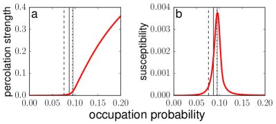
Figure 1: (Color online) Bond percolation transition of the giant connected component of the peer-to-peer Gnutella network as of August 31, 2002 Leskovec et al. (2007); Ripeanu et al. (2002). We consider the undirected version of the network, originally directed. The largest connected component is composed of $N=62,561$ nodes and $E=147,878$. a) Percolation strength $P_{\infty}$ as a function of the bond occupation probability $p$ [Eq. (1)]. b) Susceptibility $\chi$ as a function of the bond occupation probability $p$ [Eq. (2)]. $P_{\infty}$ and $\chi$ are represented as red thick lines and have been computed with $Q=10,000$ independent realizations of the Montecarlo algorithm by Newman and Ziff Newman and Ziff (2000). The best estimate of the percolation threshold $p_{c}=0.0955$ [Eq. (3), full gray line] is compared with the estimations $\tilde{p}_{c}=0.0943$ [Eq. (4), dotted black line], $\bar{p}_{c}=0.0759$ [Eq. (5), dashed black line], and $\hat{p}_{c}=0.0871$ [Eq. (6), black full line].

To this end, we first need to provide the right term of comparison, i.e., the best estimate of the true threshold by means of direct numerical simulations of the percolation process. Given an undirected and unweighted network with $N$ nodes and $E$ edges composed of a single connected component, we study bond percolation using the Montecarlo method proposed by Newman and Ziff Newman and Ziff (2000). In each realization of the method, we start from a configuration with no connections. We then sequentially add edges in random order, and monitor the evolution of the size of the largest cluster in the network $S(p)$ as a function of the bond occupation probability $p=e/E$, where $e$ indicates the number of edges added from the initial configuration, i.e., $e=0$. We repeat the entire process $Q$ independent times, and estimate the percolation strength as

$$P_{\infty}(p)=\frac{1}{N\,Q}\;\sum_{q=1}^{Q}S_{q}(p)$$ (1)

and the susceptibility as

$$\chi(p)=\frac{\frac{1}{N^{2}\,Q}\;\sum_{q=1}^{Q}S_{q}(p)S_{q}(p)-\left[P_{\infty}(p)\right]^{2}}{P_{\infty}(p)}\;,$$ (2)

where $S_{q}(p)$ indicates the size of the largest cluster in the network observed, during the $q$-th realization of the Montecarlo algorithm, when the bond occupation probability equals $p$. We determine the best estimate of the percolation threshold $p_{c}$ as the value of $p$ where the susceptibility reaches its maximum

$$p_{c}=\arg{\left\{\max_{p}\,\chi(p)\right\}}\;.$$ (3)

A concrete example of the application of the method described above to a real network is provided in Fig. 1. Note that Eq. (3) is not the only possible way to compute the best estimate of the true percolation threshold. Another very popular method is to determine $p_{c}$ as the value of $p$ where the size of the second largest cluster reaches its maximum Karrer et al. (2014). Generally, the two definitions do not provide the same exact value for the best estimates, but values whose difference is within the tolerance required for the results of this paper.

As stated above, the main purpose of our paper is to understand the best way to predict the percolation threshold of Eq. (3) without performing direct numerical simulations. We consider three different indicators. Our first estimation is based on the quantity

$$\tilde{p}_{c}=\frac{\langle k\rangle}{\langle k^{2}\rangle-\langle k\rangle}\;.$$ (4)

In Eq. (4), $\langle k\rangle$ and $\langle k^{2}\rangle$ respectively represent the first and the second moments of the degree distribution of the graph. $\tilde{p}_{c}$ represents the value of the percolation threshold expected in uncorrelated graphs with prescribed degree sequence Cohen et al. (2000); Callaway et al. (2000). In general, such prediction should fail in real networks where correlations are present. As a second prediction method of the percolation threshold, we consider the inverse of the largest eigenvalue of the adjacency matrix $A$ of the graph

$$\bar{p}_{c}=\left[\max_{\vec{v}}\,\frac{\vec{v}^{T}\,A\,\vec{v}}{\vec{v}^{T}\,\vec{v}}\right]^{-1}\;.$$ (5)

This is the expected value of the percolation threshold in graphs with a high density of connections Bollobás et al. (2010). Given that real networks are generally sparse, we expect therefore that this method is not able to produce very good prediction values of the percolation threshold. Finally, we provide an estimation of the percolation threshold as

$$\hat{p}_{c}=\left[\max_{\vec{w}}\,\frac{\vec{w}^{T}\,M\,\vec{w}}{\vec{w}^{T}\,\vec{w}}\right]^{-1}\;,$$ (6)

where the matrix $M$ is defined as

$$M=\left(\begin{array}[]{cc}A&\mathbbm{1}-D\\ \mathbbm{1}&\emptyset\end{array}\right)\;.$$ (7)

$M$ is a square matrix of dimension $2N\times 2N$ composed of four $N\times N$ blocks. $A$ is the adjacency matrix of the graph, $\mathbbm{1}$ is the identity matrix, and $D$ is a diagonal matrix whose elements are equal to the degree of the nodes. The largest eigenvalue of $M$ is identical to the largest eigenvalue of the so-called non-backtracking or Hasmimoto matrix associated with the graph Hashimoto (1989). Spectral properties of this matrix are relevant not just in percolation theory, but also for clustering algorithms and centrality measures Krzakala et al. (2013); Martin et al. (2014). The indicator of Eq. (6) is obtained in the approximation of locally tree-like networks, and it is therefore expected to provide good predictions for sparse networks Hamilton and Pryadko (2014); Karrer et al. (2014).

First, we perform a systematic study on synthetic networks. Each network realization is obtained with the use of the so-called uncorrelated configuration model Catanzaro et al. (2005). This is a variation of the model by Molloy and Reed to generate simple (i.e., without multiple or self connections) random graphs with arbitrary degree distributions Molloy and Reed (1995). In our numerical experiments, we extract degrees from the power-law probability distribution $P(k)\sim k^{-\gamma}$ if $k\in[3,\sqrt{N}]$, and $P(k)=0$, otherwise. Setting the degree cutoff at $\sqrt{N}$ ensures the absence of degree-degree correlations Boguná et al. (2004), and the correct behavior of the moments of the degree distribution Radicchi (2014). We consider six different values of the degree exponent $\gamma$, ranging from $2.1$ to $100.0$, and study the performance of $\tilde{p}_{c}$, $\bar{p}_{c}$ and $\hat{p}_{c}$ as functions of the network size $N$ (see Fig. 2). We note that for every network instance, all these quantities always provide a value smaller than $p_{c}$. We quantify the performance of a given predictor by measuring the difference between predicted value and best estimate $p_{c}$. The inverse of the largest eigenvalue of the adjacency matrix $\bar{p}_{c}$ provides reasonable predictions for the percolation threshold only for values of $\gamma<3$. In that regime, the gap $p_{c}-\bar{p}_{c}$ goes to zero, as $N$ increases, in a power-law fashion. For larger values of the degree exponent instead, the gap stabilizes to finite values even in the limit of infinitely large networks. $\tilde{p}_{c}$ and $\hat{p}_{c}$ have instead very good performances for any value of $\gamma$. Their gaps with respect to $p_{c}$ always tend to zero as the system size grows. The scaling of the gaps is well fitted by power-law functions having similar exponent values. Although $\hat{p}_{c}$ is always closer to $p_{c}$ than $\tilde{p}_{c}$, the two measures essentially provide equivalent estimates of the percolation threshold on sparse random graphs. This type of results can be understood with an intuitive mathematical argument, according to which we rewrite the eigenvalue problem for the matrix $M$ of Eq. (7) as $\left(\vec{w}_{1}^{T},\vec{w}_{2}^{T}\right)M^{T}=\lambda\left(\vec{w}_{1}^{T},\vec{w}_{2}^{T}\right)$, where $\vec{w}_{1}$ and $\vec{w}_{2}$ respectively contain the first and the second $N$ components of the eigenvector $\vec{w}$. We can now write the eigenvalue problem as two coupled equations: $A\vec{w}_{1}+(\mathbbm{1}-D)\vec{w}_{2}=\lambda\vec{w}_{1}$ and $\vec{w}_{1}=\lambda\vec{w}_{2}$. Multiplying the first equation by the row vector $\vec{u}^{T}=(1,\ldots,1)$, we obtain

$$\lambda=\frac{\vec{d}^{T}\vec{w}_{1}}{\vec{u}^{T}\vec{w}_{1}}-1\;,$$ (8)

where the components of the vector $\vec{d}$ are equal to the node degrees. In a random uncorrelated network, we should expect the non-backtracking centrality of the nodes be proportional to their degrees, i.e., $\vec{w}_{1}\sim\vec{d}$, and so Eq. (6) reduces to Eq. (4) Martin et al. (2014).

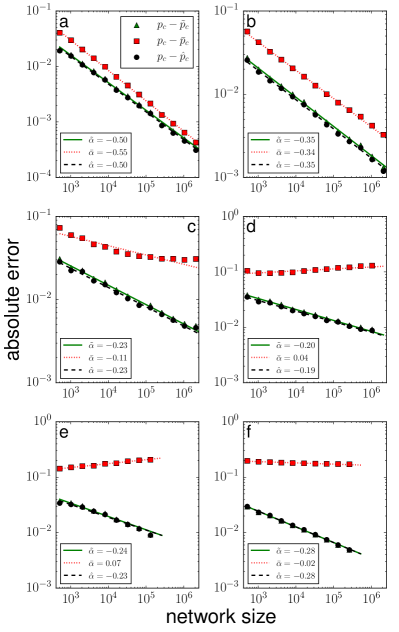
Figure 2: (Color online) Difference between best estimates of the bond percolation threshold $p_{c}$ and the predicted values $\tilde{p}_{c}$ [Eq. (4), green triangles], $\bar{p}_{c}$ [Eq. (5), red squares], and $\hat{p}_{c}$ [Eq. (6), black circles] in the uncorrelated configuration model Catanzaro et al. (2005). Gaps between best estimates and predictions are plotted as function of the network size $N$. We report results obtained for networks generated according to the power-law degree distribution $P(k)\sim k^{-\gamma}$, with support $[3,\sqrt{N}]$. Different panels correspond to different choices of the degree exponent $\gamma$: a) $\gamma=2.1$, b) $\gamma=2.5$, c) $\gamma=2.9$, d) $\gamma=3.5$, e) $\gamma=4.5$, f) $\gamma=100.0$. Points are obtained by averaging over at least $50$ independent network instances. Standard errors on the measures have size smaller than those of the symbols. For each network, the best estimate of the bond percolation threshold is obtained with $Q=100$ Montecarlo realizations of the Newman-Ziff algorithm Newman and Ziff (2000). In the various panels, lines correspond to best fits of the empirical points with the functions $p_{c}-\tilde{p}_{c}\sim N^{\tilde{\alpha}}$ (full green lines), $p_{c}-\bar{p}_{c}\sim N^{\bar{\alpha}}$ (red dotted lines), and $p_{c}-\hat{p}_{c}\sim N^{\hat{\alpha}}$ (black dashed lines).

Second and more importantly, we perform a systematic study of the predictive power of $\tilde{p}_{c}$, $\bar{p}_{c}$ and $\hat{p}_{c}$ in a collection of $109$ real networks. We consider graphs of heterogeneous nature, including biological, infrastructural, information, technological, social, and communication networks, and thus very variegate also in terms of structural properties (e.g., degree distribution and correlations, clustering coefficient, diameter). In our numerical study, we reduce, if necessary, weighted and/or directed networks to their unweighted and undirected projections. Also, we focus our attention only to their giant connected components. Results for all $109$ real networks are provided in the Supplemental Material. In Fig. 3, we summarize the main outcome of our analysis. As expected, both $\bar{p}_{c}$ and $\hat{p}_{c}$ always provide a lower bound for $p_{c}$ Karrer et al. (2014). Since we have by definition $\hat{p}_{c}\geq\bar{p}_{c}$, it is not a big surprise to find that $\hat{p}_{c}$ generates always better predictions than $\bar{p}_{c}$ Karrer et al. (2014). It is however worth to remark that, whereas in synthetic networks the difference between the inverse of the largest eigenvalue of the adjacency matrix $\bar{p}_{c}$ and $\hat{p}_{c}$ can be very large, in real networks, the two indicators generate pretty similar estimations of the percolation threshold, suggesting a relatively little advantage in using $\hat{p}_{c}$ in place of $\bar{p}_{c}$ (see Supplemental Material). It is interesting to observe that, in about the $40\%$ of the real networks analyzed, the naive estimator $\tilde{p}_{c}$, based only on the fraction between first and second moments on the degree distribution, outperforms $\hat{p}_{c}$ in spite of using much less topological information. On the other hand, the use of $\tilde{p}_{c}$ as prediction tool has the disadvantage of alternatively over- or under- estimate the value of the percolation threshold. The relative error of $\hat{p}_{c}$ is an increasing function of the percolation threshold $p_{c}$. $\tilde{p}_{c}$ approximates better $p_{c}$ as the percolation threshold increases. Also, the performances of the indicators do not seem to be strongly related to the edge density of graph (see Supplemental Material). Overall, the predictive power of $\tilde{p}_{c}$ is lower than the one of $\hat{p}_{c}$, as $\tilde{p}_{c}$ often predicts too low values of the percolation threshold.

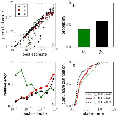
Figure 3: (Color online) Comparison between best estimates and predicted values of the percolation threshold of $109$ real networks. In each network, the best estimate $p_{c}$ of the percolation threshold [Eq. (3)] is computed with $Q=10,000$ independent realizations of the Montecarlo method by Newman and Ziff Newman and Ziff (2000). a) For each network, we plot [Eq. (4), green triangles], $\bar{p}_{c}$ [Eq. (5, red squares], and $\hat{p}_{c}$ [Eq. (6), black circles] as functions of the best estimate $p_{c}$. The black dashed line represents perfect agreement between predicted values and best estimates. b) Probability, computed over the entire sample of real networks, that either $\tilde{p}_{c}$ (green) or $\hat{p}_{c}$ assume the closest value to $p_{c}$. c) Relative error of the three predictors, with respect to the value of the best estimate, as function of $p_{c}$. We use the same symbols and colors as those of panel a. d) Cumulative distribution of the relative error between predictions and best estimates. Green dotted line refers to $\tilde{p}_{c}$, red full line to $\bar{p}_{c}$, and black dashed line to $\hat{p}_{c}$. Global performances of the prediction methods are measured in terms of the area under the curve (AUC).

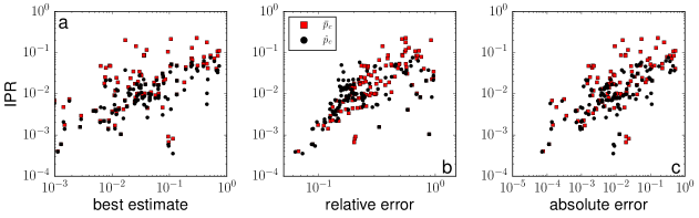
Figure 4: (Color online) Inverse participation ratio (IPR) of the principal eigenvectors of the adjacency (red squares) and the non-backtracking matrices [Eq. 7, black circles] as functions of the value of the best estimate of the percolation threshold $p_{c}$ (panel a), the relative error (panel b), and the absolute error (panel c). Each point refers to numerical results obtained on one of the $109$ real networks considered in our analysis.

On the basis of our results, we can conclude that the inverse of the largest eigenvalue of the non-backtracking matrix $\hat{p}_{c}$ represents the best measure currently available on the market, among those that do not rely on direct numerical simulations of the percolation process, to provide estimates of the bond percolation threshold $p_{c}$ in an arbitrary network. Apparently, its predictive power is not much influenced by the density of edges, as long as the network is sufficiently sparse. Performances are instead strongly dependent on the value of the true percolation threshold. $\hat{p}_{c}$ generates particularly good prediction values for bond percolation thresholds in networks, if threshold values are sufficiently small. On the other hand, it fails by non negligible amounts, if the true percolation threshold is large. This fact substantially happens for infrastructural networks, such as road networks Leskovec et al. (2009) and power grids Watts and Strogatz (1998), off-line social networks Zachary (1977); Lusseau et al. (2003); Milo et al. (2004), and biological networks Milo et al. (2004) (see Supplemental Material). Also, this fact often happens in networks with double percolation transitions colomer , where $\hat{p}_{c}$ tends to predict the lower threshold that does not necessarily coincide with the largest jump of the percolation strength.

The inadequacy of the indicator $\hat{p}_{c}$ to provide good predictions for $p_{c}$ in the regime of large percolation thresholds may be related to the localization of the eigenvector associated with the principal eigenvalue of the matrix defined in Eq. (7). Since the second $N$ components of any eigenvector of the matrix $M$ are proportional to the first $N$, we quantify the localization of such eigenvector by normalizing the first $N$ components (i.e., the sum of their squares equals one), and then computing its inverse participation ratio, defined as the sum of the fourth power of the components. Our measures performed on real networks indicate the presence of a positive correlation between the value of the inverse participation ratio and the value of the best estimate of the percolation threshold $p_{c}$ (Fig.4a). They also show a positive correlation between the inverse participation ratio and the relative and absolute errors of $\hat{p}_{c}$ with respect to $p_{c}$ (Figs.4b and c). Thus the reason of the bad performance of $\hat{p}_{c}$ seems analogous to the one valid for spectral estimators of epidemic thresholds in real networks Goltsev et al. (2012). Mathematically speaking when the principal eigenvector is localized, the percolation transition placed at $\hat{p}_{c}$ involves in reality only a finite fraction of the nodes in the network, and thus does not correspond to the true percolation transition located instead at $p_{c}$. The same type of considerations stressed for the principal eigenvector of the non-backtracking matrix can be also extended to the principal eigenvector of the adjacency matrix to motivate why $\bar{p}_{c}$ suffers from the same limitations as those observed for $\hat{p}_{c}$ (Fig. 4).

As a final consideration, we would like to stress that the existence of a positive relation between the error committed by $\hat{p}_{c}$ to predict $p_{c}$ and the value of $p_{c}$ itself is an important limitation for the use of $\hat{p}_{c}$ as a proxy for network robustness. In this context, percolation is better thought by removing than adding edges, so that the robustness of a network is given by $1-p_{c}$. The prediction $1-\hat{p}_{c}$ always overestimates the true fraction of edge failures that a system can tolerate, providing therefore an information not useful to prevent catastrophic events. Even more importantly, in the analysis of network resilience to random attacks, it is generally more meaningful to consider site instead of bond percolation. Site percolation thresholds are larger than those valid for the edges (see Supplemental Material), and $1-\hat{p}_{c}$ seems not able to provide sufficiently accurate predictions for the maximal number of vertices that can be removed from a network before reaching system failure. For all these reasons, we believe that additional theoretical efforts must be devoted to the search of good predictors able to determine tight upper bounds of percolation thresholds in networks.