GRAVITY WAVES FROM NON-MINIMAL QUADRATIC INFLATION

Abstract

We discuss non-minimal quadratic inflation in supersymmetric (SUSY) and non-SUSY models which entails a linear coupling of the inflaton to gravity. Imposing a lower bound on the parameter $c_{\cal R}$, involved in the coupling between the inflaton and the Ricci scalar curvature, inflation can be attained even for subplanckian values of the inflaton while the corresponding effective theory respects the perturbative unitarity up to the Planck scale. Working in the non-SUSY context we also consider radiative corrections to the inflationary potential due to a possible coupling of the inflaton to bosons or fermions. We find ranges of the parameters, depending mildly on the renormalization scale, with adjustable values of the spectral index $n_{\rm s}$, tensor-to-scalar ratio $r\simeq(2-4)\cdot 10^{-3}$, and an inflaton mass close to $3\cdot 10^{13}~{}{\mbox{\rm GeV}}$. In the SUSY framework we employ two gauge singlet chiral superfields, a logarithmic Kähler potential including all the allowed terms up to fourth order in powers of the various fields, and determine uniquely the superpotential by applying a continuous $R$ and a global $U(1)$ symmetry. When the Kähler manifold exhibits a no-scale-type symmetry, the model predicts $n_{\rm s}\simeq 0.963$ and $r\simeq 0.004$. Beyond no-scale SUGRA, $n_{\rm s}$ and $r$ depend crucially on the coefficient involved in the fourth order term, which mixes the inflaton with the accompanying non-inflaton field in the Kähler potential, and the prefactor encountered in it. Increasing slightly the latter above $(-3)$, an efficient enhancement of the resulting $r$ can be achieved putting it in the observable range. The inflaton mass in the last case is confined in the range $(5-9)\cdot 10^{13}~{}{\mbox{\rm GeV}}$.

Keywords: Cosmology, Supersymmetric models, Supergravity;
PACS codes: 98.80.Cq, 11.30.Qc, 12.60.Jv, 04.65.+e

Published in J. Cosmol. Astropart. Phys. 03, 023 (2015)

1 Introduction

The simplest model [1] of chaotic inflation (CI) based on a quadratic potential predicts a (scalar) spectral index $n_{\rm s}\simeq 0.963$ (in good agreement with WMAP [2] and Planck [3] measurements) and a tensor-to-scalar ratio $r$, a canonical measure of primordial gravity waves, close to $0.15$ or so. The Bicep2 results [4] announced earlier this year, purporting to have found gravity waves from inflation ($r\simeq 0.16$) provided a huge boost for this class of models [5, 6, 7, 8, 9]. However, serious doubts regarding the Bicep2 results have appeared in the literature [10, 11] that are largely related to the inadequate treatment of the impact on their analysis of the dust background. Furthermore, very recently, the Planck HFI 353 GHz dust polarization data [12] has been released and the first attempts to make a joint analysis of Planck and Bicep2 data have been presented [11, 13] concluding that the quadratic CI is disfavored at more than 95$\%$ confidence level (c.l.). Indeed, it is conceivable that most, if not the whole, Bicep2  polarization signal may be caused by the dust.

Be that as it may, it was shown several years ago [14] that a quadratic (or quartic) potential can, at best, function as an approximation within a more realistic inflationary cosmology. The end of CI is followed by a reheating phase which is implemented through couplings involving the inflaton and some additional suitably selected fields. The presence of these additional couplings can significantly modify, through radiative corrections (RCs), the tree level inflationary potential. For instance, for a quadratic potential supplemented by a coupling of the inflation field to, say, right-handed neutrinos, $r$ can be reduced to values close to $0.05$ [5] or so, at the cost of a (less efficient) reduction of $n_{\rm s}$, though. In this paper we briefly review this idea taking into account the recent refinements of Ref. [15], according to which an unavoidable dependence of the results on the renormalization scale arises.

Another mechanism for reducing $r$ at an acceptable level within models of quadratic CI is the introduction of a strong, linear non-minimal coupling of the inflaton to gravity [17, 16]. The aforementioned mechanism, that we mainly pursue here, can be applied either within a supersymmetric (SUSY) [16] or a non-SUSY [17] framework. The resulting inflationary scenario, named non-minimal CI (nMI), belongs to a class of universal “attractor” models [18], in which an appropriate choice of the non-minimal coupling to gravity suitably flattens the inflationary potential, such that $r$ is heavily reduced but $n_{\rm s}$ stays close to the currently preferred value of $0.96$. However, in generic Supergravity (SUGRA) settings, a mild tuning is needed [19] respecting the coefficient $k_{S\Phi}$ involved in the fourth order term that mixes the inflaton with the accompanying non-inflaton field in the Kähler potential.

In this work we reexamine the realization of nMI based on the quadratic potential implementing the following improvements:

• As regards the non-SUSY case, we also consider RCs to the tree-level potential which arise due to Yukawa interactions of the inflaton – cf. Ref. [20, 21]. We show that the presence of RCs can affect the $n_{\rm s}$ values of nMI – in contrast to minimal CI, where RCs influence both $n_{\rm s}$ and $r$. For subplanckian values of the inflaton field, though, $r$ remains well suppressed and may be observable only in the next generation of experiments such as COrE+ [22], PIXIE [23] and LiteBIRD [24] which may bring the sensitivity down to $10^{-3}$.

• As regards the SUSY case, following Ref. [25], we generalize the embedding of the model in SUGRA allowing for a variation of the numerical prefactor encountered in the adopted Kähler potential. We show that (i) the tuning of $k_{S\Phi}$ can be totally avoided in the case of no-scale SUGRA which uniquely predicts $n_{\rm s}\simeq 0.963$ and $r\simeq 0.004$; (ii) beyond no-scale SUGRA, increasing slightly the prefactor $(-3)$ encountered in the adopted Kähler potential and adjusting appropriately $k_{S\Phi}$, an efficient enhancement of the resulting $r$, for any $n_{\rm s}$, can be achieved which will be tasted in the near future [26, 27].

We finally show that, in both of the above cases, the ultaviolet (UV) cut-off scale [28, 29] of the theory can be identified with the Planck scale and, thus, concerns regarding the naturalness of this kind of nMI can be safely evaded. It is worth emphasizing that this nice feature of these models was recently noticed in Ref. [30] and was not recognized in the original papers [17, 16].

The paper is organized as follows: In Sec. 2, we describe the generic formulation of CI with a quadratic potential and a non-minimal coupling to gravity. The emergent non-SUSY and SUSY inflationary models are analyzed in Secs. 3 and 4 respectively. The UV behavior of these models is analyzed in Sec. 5 and our conclusions are summarized in Sec. 6. In Appendix A we outline the implementation of nMI by the imaginary part of the inflaton superfield adopting a shift-symmetric logarithmic Kähler potential. Throughout the text, the symbol $,\chi$ as subscript denotes derivation with respect to (w.r.t) the field $\chi$ (e.g., ${}_{,\chi\chi}=\partial^{2}/\partial\chi^{2}$); charge conjugation is denoted by a star, and we use units where the reduced Planck scale $M_{\rm P}=2.43\cdot 10^{18}~{}{\mbox{\rm GeV}}$ is set equal to unity.

2 Inflaton non-Minimally Coupled to Gravity

We consider below an inflationay sector coupled non-minimally to gravity within a non-SUSY (Sec. 2.1) or a SUSY (Sec. 2.2) framework. Based on this formulation, we then derive the inflationary observables and impose the relevant observational constraints in Sec. 2.3.

2.1 non-SUSY Framework

In the Jordan frame (JF) the action of an inflaton $\phi$ with potential $V_{\rm CI}\left(\phi\right)$ non-minimally coupled to the Ricci scalar $\mathcal{R}$ through a coupling function $f_{\cal R}(\phi)$ has the form:

$${\sf S}=\int d^{4}x\sqrt{-\mathfrak{g}}\left(-\frac{1}{2}f_{\cal R}\mathcal{R}+\frac{f_{K}}{2}g^{\mu\nu}\partial_{\mu}\phi\partial_{\nu}\phi-V_{\rm CI0}+\mathcal{L}_{\rm int}\right),$$ (1)

where $\mathfrak{g}$ is the determinant of the background Friedmann-Robertson-Walker metric, $g^{\mu\nu}$. We allow also for a kinetic mixing through the function $f_{K}(\phi)$ and a part of the langrangian $\mathcal{L}_{\rm int}$ which is responsible for the interaction of $\phi$ with a boson $\chi$ and a fermion $\psi$, i.e.,

$$\mathcal{L}_{\rm int}=\frac{1}{2}g_{\chi}\phi^{2}\chi^{2}+g_{\psi}\phi\bar{\psi}\psi\,.$$ (2)

By performing a conformal transformation [17] according to which we define the Einstein frame (EF) metric

$$\widehat{g}_{\mu\nu}=f_{\cal R}\,g_{\mu\nu}~{}~{}\Rightarrow~{}~{}\left\{\begin{matrix}\sqrt{-\widehat{\mathfrak{g}}}=f_{\cal R}^{2}\sqrt{-\mathfrak{g}}\hskip 5.69046pt\mbox{and}\hskip 5.69046pt\widehat{g}^{\mu\nu}=g^{\mu\nu}/f_{\cal R}\,\hfill\cr\widehat{}\mathcal{R}=\left(\mathcal{R}+3\Box\ln f_{\cal R}+3g^{\mu\nu}\partial_{\mu}f_{\cal R}\partial_{\nu}f_{\cal R}/2f_{\cal R}^{2}\right)/f_{\cal R}\,\hfill\cr\end{matrix}\right.\,,$$ (3)

where $\Box=\left(-\mathfrak{g}\right)^{-1/2}\partial_{\mu}\left(\sqrt{-\mathfrak{g}}\partial^{\mu}\right)$ and hat is used to denote quantities defined in the EF, we can write ${\sf S}$ in the EF as follows:

$${\sf S}=\!\int d^{4}x\sqrt{-\widehat{\mathfrak{g}}}\left(-\frac{1}{2}\widehat{\mathcal{R}}+\frac{1}{2}\widehat{g}^{\mu\nu}\partial_{\mu}\widehat{\phi}\partial_{\nu}\widehat{\phi}-\widehat{V}_{\rm CI0}+\widehat{\mathcal{L}}_{\rm int}\right)\,.$$ (4)

The EF canonically normalized field, $\widehat{\phi}$, the EF potential, $\widehat{V}_{\rm CI}$, and the interaction Langrangian, $\widehat{\mathcal{L}}_{\rm int}$ turn out to be:

$$\mbox{\footnotesize\sf(a)}\>\>\>\left(\frac{d\widehat{\phi}}{d\phi}\right)^{2}=J^{2}=\frac{f_{K}}{f_{\cal R}}+{3\over 2}\left({f_{{R},\phi}\over f_{\cal R}}\right)^{2},\>\>\>\mbox{\footnotesize\sf(b)}\>\>\>\widehat{V}_{\rm CI0}=\frac{V_{\rm CI0}}{f_{\cal R}^{2}}~{}~{}\mbox{and}~{}~{}\mbox{\footnotesize\sf(c)}\>\>\>\widehat{\mathcal{L}}_{\rm int}=\frac{\mathcal{L}_{\rm int}}{f_{\cal R}^{2}}\,\cdot$$ (5)

Taking into account that $\widehat{\chi}=f_{\cal R}^{-1/2}\chi$, $\widehat{\psi}=f_{\cal R}^{-3/4}\psi~{}~{}\Rightarrow~{}~{}\overline{\widehat{\psi}}=f_{\cal R}^{-3/4}{\bar{\psi}}$ [31], and that the masses of these particles during CI are heavy enough such that the dependence of $f_{\cal R}$ on $\phi$ does not influence their dynamics, $\widehat{\mathcal{L}}_{\rm int}$ can be written as

$$\widehat{\mathcal{L}}_{\rm int}=\frac{g_{\chi}\phi^{2}}{2f_{\cal R}}\,\widehat{\chi}^{2}+\frac{g_{\psi}\phi}{\sqrt{f_{\cal R}}}\,\overline{\widehat{\psi}}\,\widehat{\psi}\,.$$ (6)

From Eq. (5) we infer that convenient choices of $V_{\rm CI}$ and $f_{\cal R}$ assist us to obtain $\widehat{V}_{\rm CI}$ suitable for observationally consistent CI. Focusing on quadratic CI and following Ref. [17, 18], we select

$$\mbox{\footnotesize\sf(a)}\>\>\>V_{\rm CI0}={1\over 2}m^{2}\phi^{2}\>\>\>\mbox{\footnotesize\sf(b)}\>\>\>f_{\cal R}(\phi)=1+c_{\cal R}\phi\>\>\>\mbox{and}\>\>\mbox{\footnotesize\sf(c)}\>\>\>f_{K}=1$$ (7)

where $m$ is the renormalized mass of the inflaton. For $c_{\cal R}\gg 1$ we observe that a sufficiently flat $\widehat{V}_{\rm CI0}$ through Eq. (5b) can be obtained which may decrease $r$ from its value in (minimal) quadratic CI. On the other hand, the vacuum expectation value (v.e.v) of $\phi$ is $\langle{\phi}\rangle=0$, and the validity of ordinary Einstein gravity is guaranteed since $\langle{f_{\cal R}}\rangle=1$.

2.2 SUGRA Framework

A convenient implementation of nMI in SUGRA is achieved by employing two singlet superfields, i.e., $z^{\alpha}=\Phi,S$, with $\Phi$ (${\alpha}=1$) and $S$ (${\alpha}=2)$ being the inflaton and a “stabilized” field respectively. The EF action for $z^{\alpha}$’s within SUGRA [32] can be written as

$${\sf S}=\int d^{4}x\sqrt{-\widehat{\mathfrak{g}}}\left(-\frac{1}{2}\widehat{\mathcal{R}}+K_{{\alpha}{\bar{\beta}}}\widehat{g}^{\mu\nu}\partial_{\mu}z^{\alpha}\partial_{\nu}z^{*{\bar{\beta}}}-\widehat{V}\right),$$ (8a)

where the summation is taken over the scalar fields $$z^{\alpha} K_{{\alpha}{\bar{\beta}}}={K_{,z^{\alpha}z^{*{\bar{\beta}}}}} K^{{\bar{\beta}}{\alpha}}K_{{\alpha}\bar{\gamma}}=\delta^{\bar{\beta}}_{\bar{\gamma}} \widehat{\mathfrak{g}} \widehat{g}_{\mu\nu} \widehat{\mathcal{R}} \widehat{V} W K$$, with , is the determinant of the EF metric , is the EF Ricci scalar curvature, is the EF F–term SUGRA scalar potential which can be extracted once the superpotential and the Kähler potential  have been selected, by applying the standard formula

$$\widehat{V}=e^{K}\left(K^{{\alpha}{\bar{\beta}}}{\rm F}_{\alpha}{\rm F}^{*}_{\bar{\beta}}-3{|W|^{2}}\right),\>\>\>\mbox{where}\>\>\>{\rm F}_{\alpha}=W_{,z^{\alpha}}+K_{,z^{\alpha}}W.$$ (8b)

Note that D-term contributions to $\widehat{V}$ do not exist since we consider gauge singlet $z^{\alpha}$’s.

A quadratic potential for $\Phi$ in this setting can be realized if we adopt the following superpotential

$$W=mS\Phi\,.$$ (9)

To protect the form of $W$ from higher order terms we impose two symmetries: Firstly, an $R$ symmetry under which $S$ and $\Phi$ have charges $1$ and $0$ respectively, which ensures the linearity of $W$ w.r.t $S$; secondly, a global $U(1)$ symmetry with assigned charges $-1$ and $1$ for $S$ and $\Phi$ respectively. To verify that $W$ leads to the desired quadratic potential we present the SUSY limit, $V_{\rm SUSY}$ of $\widehat{V}$, which is

$$V_{\rm SUSY}=m^{2}\left(|\Phi|^{2}+|S|^{2}\right).$$ (10a)

Note that the complex scalar components of $$\Phi S S V_{\rm SUSY} \Phi$$ and superfields are denoted by the same symbol. From Eq. (10a), we can easily conclude that for stabilized to zero, becomes quadratic w.r.t to the real (or imaginary) part of . The SUSY vacuum lies at

$$\langle{S}\rangle=\langle{\Phi}\rangle=0.$$ (10b)

The construction of Eq. (1) can be obtained within SUGRA if we perform the inverse of the conformal transformation described in Eq. (3) with

$$f_{\cal R}=-\Omega/3(1+n),$$ (11)

and specify the following relation between $K$ and $\Omega$,

$$-\Omega/3(1+n)=e^{-K/3(1+n)}\>\Rightarrow\>K=-3(1+n)\ln\left(-\Omega/3(1+n)\right)\,.$$ (12)

Here $n$ is a dimensionless (small in our approach) parameter which quantifies the deviation from the standard set-up [32]. Following Ref. [25] we arrive at the following action

$${\sf S}=\int d^{4}x\sqrt{-\mathfrak{g}}\left(\frac{\Omega\mathcal{R}}{6(1+n)}+\left(\Omega_{{\alpha}{{\bar{\beta}}}}-\frac{n\Omega_{{\alpha}}\Omega_{{\bar{\beta}}}}{(1+n)\Omega}\right)\partial_{\mu}z^{\alpha}\partial^{\mu}z^{*{\bar{\beta}}}-\frac{\Omega{\cal A}_{\mu}{\cal A}^{\mu}}{(1+n)^{3}}-V\right),$$ (13)

where $V=\Omega^{2}\widehat{V}/9(1+n)^{2}$ is the JF potential and ${\cal A}_{\mu}$ is [32] the purely bosonic part of the on-shell value of the auxiliary field

$${\cal A}_{\mu}=-i(1+n)\left(\Omega_{\alpha}\partial_{\mu}z^{\alpha}-\Omega_{\bar{\alpha}}\partial_{\mu}z^{*{\bar{\alpha}}}\right)/2\Omega\,.$$ (14)

It is clear from Eq. (13) that ${\sf S}$ exhibits non-minimal couplings of the $z^{\alpha}$’s to $\mathcal{R}$. However, $\Omega$ also enters the kinetic terms of the $z^{\alpha}$’s. To separate the two contributions we split $\Omega$ into two parts

$$-\Omega/3(1+n)=\Omega_{\rm H}(\Phi)+{\Omega_{\rm H}}^{*}(\Phi^{*})-\Omega_{\rm K}\left(|\Phi|^{2},|S|^{2}\right)/3(1+n),$$ (15a)

where $$\Omega_{\rm K} z^{\alpha}$$ is a dimensionless real function including the kinetic terms for the ’s and takes the form

$$\Omega_{\rm K}\left(|\Phi|^{2},|S|^{2}\right)={k_{\sf NS}|\Phi|^{2}+|S|^{2}}\,-\,2\left(k_{S}|S|^{4}+k_{\Phi}|\Phi|^{4}+k_{S\Phi}|S|^{2}|\Phi|^{2}\right)\,,$$ (15b)

with coefficients $$k_{\sf NS},k_{S},k_{\Phi} k_{S\Phi} S 2 \Omega_{\rm H} \Omega_{\rm H}>\Omega_{\rm K} \Omega_{{\alpha}{{\bar{\beta}}}} \Omega_{\rm H} \Omega_{{\rm H},z^{\alpha}z^{*{\bar{\beta}}}}=0$$ and of order unity. The fourth order term for is included to cure the problem of a tachyonic instability occurring along this direction [32], and the remaining terms of the same order are considered for consistency – the factors of are added just for convenience. Alternative solutions to the aforementioned problem of the tachyonic instability are recently identified in Ref. [33, 34]. On the other hand, in Eq. (15a) is a dimensionless holomorphic function which, for , represents the non-minimal coupling to gravity – note that is independent of since . To obtain a situation similar to Eq. (7), we adopt

$$\Omega_{\rm H}=\frac{1}{2}+{c_{\cal R}\over\sqrt{2}}\Phi\,,$$ (15c)

which respects the imposed $R$ symmetry but explicitly breaks $U(1)$ during nMI. Furthermore, assuming that the phase of $\Phi$, ${\small\sf arg}\Phi$, is stabilized to zero, the selected $\Omega_{\rm H}$ at the SUSY vacuum, Eq. (10b), reads

$$-\langle{\Omega}\rangle/3(1+n)=1\,,$$ (16)

which ensures a recovery of conventional Einstein gravity at the end of nMI.

When the dynamics of the $z^{\alpha}$’s is dominated only by the real moduli $|z^{\alpha}|$, or if $z^{\alpha}=0$ for ${\alpha}\neq 1$ [32], we can obtain ${\cal A}_{\mu}=0$ in Eq. (13). The choice $n\neq 0$, although not standard, is perfectly consistent with the idea of nMI. Indeed, the only difference occurring for $n\neq 0$ – compared to the $n=0$ case – is that the $z^{\alpha}$’s do not have canonical kinetic terms in the JF due to the term proportional to $\Omega_{\alpha}\Omega_{\bar{\beta}}\neq\delta_{{\alpha}{\bar{\beta}}}$. This fact does not cause any problem since the canonical normalization of $\Phi$ keeps its strong dependence on $c_{\cal R}$ included in $\Omega_{\rm H}$, whereas $S$ becomes heavy enough during nMI and so it does not affect the dynamics – see Sec. 4.1.

In conclusion, through Eq. (12) the resulting Kähler potential is

$$K=-3(1+n)\ln\left(1+{c_{\cal R}\over\sqrt{2}}\left(\Phi+\Phi^{*}\right)-{|S|^{2}+k_{\sf NS}|\Phi|^{2}\over 3(1+n)}+2{k_{S}|S|^{4}+k_{\Phi}|\Phi|^{4}+k_{S\Phi}|S|^{2}|\Phi|^{2}\over 3(1+n)}\right).$$ (17)

We set $k_{\sf NS}=1$ throughout, except for the case of no-scale SUGRA which is defined as follows:

$$n=0,\>\>\>k_{\sf NS}=0\>\>\>\mbox{and}\>\>\>k_{S\Phi}=k_{\Phi}=0\,.$$ (18)

This arrangement, inspired by the early models of soft SUSY breaking [35, 36], corresponds to the Kähler manifold $SU(2,1)/SU(2)\times U(1)_{R}$ with constant curvature equal to $-2/3$. In practice, these choices highly simplify the realization of nMI, thus rendering it more predictive thanks to a lower number of the remaining free parameters.

2.3 Inflationary Observables – Constraints

The analysis of nMI can be carried out exclusively in the EF using the standard slow-roll approximation keeping in mind the dependence of $\widehat{\phi}$ on $\phi$ – given by Eq. (5) in both the SUSY and non-SUSY set-up. Working this way, in the following we outline a number of observational requirements with which any successful inflationary scenario must be compatible – see, e.g., Ref. [37].

2.3.1.

The number of e-folds, $\widehat{N}_{\star}$, that the scale $k_{\star}=0.05/{\rm Mpc}$ experiences during CI,

$$\widehat{N}_{\star}=\int_{\widehat{\phi}_{\rm f}}^{\widehat{\phi}_{\star}}\,d\widehat{\phi}\>\frac{\widehat{V}_{\rm CI}}{\widehat{V}_{\rm CI,\widehat{\phi}}}=\int_{\phi_{\rm f}}^{\phi_{\star}}\,J^{2}\frac{\widehat{V}_{\rm CI}}{\widehat{V}_{\rm CI,\phi}}{d\phi},$$ (19)

must be enough to resolve the horizon and flatness problems of standard big bang, i.e., [39, 3]

$$\widehat{N}_{\star}\simeq 61.7+\ln{\widehat{V}_{\rm CI}(\phi_{\star})^{1/2}\over\widehat{V}_{\rm CI}(\phi_{\rm f})^{1/3}}+{1\over 3}\ln T_{\rm rh}+{1\over 2}\ln{f_{\cal R}(\phi_{\star})\over f_{\cal R}(\phi_{\rm f})^{1/3}},$$ (20)

where $\widehat{V}_{\rm CI}$ is the radiatively corrected EF potential presented in Sec. 3.1 [Sec. 4.1] for the non-SUSY [SUSY] scenario. Also, we assume here that nMI is followed in turn by a decaying-inflaton, radiation and matter domination, $T_{\rm rh}$ is the reheat temperature after nMI, $\phi_{\star}~{}[\widehat{\phi}_{\star}]$ is the value of $\phi~{}[\widehat{\phi}]$ when $k_{\star}$ crosses outside the inflationary horizon, and $\phi_{\rm f}~{}[\widehat{\phi}_{\rm f}]$ is the value of $\phi~{}[\widehat{\phi}]$ at the end of nMI. The latter can be found, in the slow-roll approximation for the models considered in this paper, from the condition

$${\sf max}\{\widehat{\epsilon}(\phi_{\rm f}),|\widehat{\eta}(\phi_{\rm f})|\}=1,$$ (21a)

where the slow-roll parameters can be calculated as follows:

$$\widehat{\epsilon}={1\over 2}\left(\frac{\widehat{V}_{\rm CI,\widehat{\phi}}}{\widehat{V}_{\rm CI}}\right)^{2}={1\over 2J^{2}}\left(\frac{\widehat{V}_{\rm CI,\phi}}{\widehat{V}_{\rm CI}}\right)^{2}\>\>\>\mbox{and}\>\>\>\>\>\widehat{\eta}=\frac{\widehat{V}_{\rm CI,\widehat{\phi}\widehat{\phi}}}{\widehat{V}_{\rm CI}}={1\over J^{2}}\left(\frac{\widehat{V}_{\rm CI,\phi\phi}}{\widehat{V}_{\rm CI}}-\frac{\widehat{V}_{\rm CI,\phi}}{\widehat{V}_{\rm CI}}{J_{,\phi}\over J}\right)\cdot$$ (21b)

It is worth mentioning that in our approach we calculate $\widehat{N}_{\star}$ self-consistently with $\widehat{V}_{\rm CI}$ and $T_{\rm rh}$, and do not let it vary within the interval $50-60$ as often done in the literature – see e.g. Ref. [3, 5]. Our estimation for $\widehat{N}_{\star}$ in Eq. (20) takes into account the transition from the JF to EF – see Ref. [17] – and the assumption that nMI is followed in turn by a decaying-particle, radiation and matter domination – for details see Ref. [38]. During the first period, we adopt the so-called [39] canonical reheating scenario with an effective equation-of-state parameter $w_{\rm re}=0$. This value corresponds precisely to the equation-of-state parameter, $w$, for a quadratic potential. In the nMI case we expect that $w$ will deviate slightly from this value. However, this effect is quite negligible since for low $\phi$ values the inflationary potential can be well approximated by a quadratic potential – see Sec. 5 below.

2.3.2.

The amplitude $A_{\rm s}$ of the power spectrum of the curvature perturbation generated by $\phi$ at the pivot scale $k_{\star}$ must be consistent with data [3]:

$$\sqrt{A_{\rm s}}=\>\frac{1}{2\sqrt{3}\,\pi}\;\frac{\widehat{V}_{\rm CI}(\widehat{\phi}_{\star})^{3/2}}{|\widehat{V}_{\rm CI,\widehat{\phi}}(\widehat{\phi}_{\star})|}=\frac{|J(\phi_{\star})|}{2\sqrt{3}\,\pi}\;\frac{\widehat{V}_{\rm CI}(\phi_{\star})^{3/2}}{|\widehat{V}_{\rm CI,\phi}(\phi_{\star})|}\simeq 4.685\cdot 10^{-5},$$ (22)

where we assume that no other contributions to the observed curvature perturbation exists.

2.3.3.

The (scalar) spectral index, $n_{\rm s}$, its running, $a_{\rm s}$, and the scalar-to-tensor ratio $r$ must be in agreement with the fitting of the data [3] with $\Lambda$CDM model, i.e.,

$$\mbox{\footnotesize\sf(a)}\>\>\>n_{\rm s}=0.9603\pm 0.0146,\>\>\>\mbox{\footnotesize\sf(b)}\>\>\>-0.0314\leq a_{\rm s}\leq 0.0046\>\>\>\mbox{and}\>\>\>\mbox{\footnotesize\sf(c)}\>\>\>r<0.1\>\>\>\mbox{at 95$\%$.}$$ (23)

In Eq. (23c) we conservatively take into account the recent analyses [11, 13] which combine the Bicep2 results [4] with the polarized foreground maps released by Planck [12]. These observables are estimated through the relations:

$$\mbox{\footnotesize\sf(a)}\>\>\>n_{\rm s}=\>1-6\widehat{\epsilon}_{\star}\ +\ 2\widehat{\eta}_{\star},\>\>\>\mbox{\footnotesize\sf(b)}\>\>\>a_{\rm s}=\>2\left(4\widehat{\eta}_{\star}^{2}-(n_{\rm s}-1)^{2}\right)/3-2\widehat{\xi}_{\star}\>\>\>\mbox{and}\>\>\>\mbox{\footnotesize\sf(c)}\>\>\>r=16\widehat{\epsilon}_{\star},$$ (24)

where $\widehat{\xi}={\widehat{V}_{\rm CI,\widehat{}\phi}\widehat{V}_{\rm CI,\widehat{}\phi\widehat{}\phi\widehat{}\phi}/\widehat{V}^{2}}=\,\widehat{V}_{\rm CI,\phi}\,\widehat{\eta}_{,\phi}/\widehat{V}_{\rm CI}\,J^{2}+2\widehat{\eta}\widehat{\epsilon}$ and the variables with subscript $\star$ are evaluated at $\phi=\phi_{\star}$.

2.3.4.

To avoid corrections from quantum gravity and any destabilization of our inflationary scenario due to higher order terms – e.g. in Eq. (7) or Eq. (15c) –, we impose two additional theoretical constraints on our models – keeping in mind that $\widehat{V}_{\rm CI}(\phi_{\rm f})\leq\widehat{V}_{\rm CI}(\phi_{\star})$:

$$\mbox{\footnotesize\sf(a)}\>\>\widehat{V}_{\rm CI}(\phi_{\star})^{1/4}\leq 1\>\>\>\mbox{and}\>\>\>\mbox{\footnotesize\sf(b)}\>\>\phi_{\star}\leq 1.$$ (25)

As we show in Sec. 5, the UV cutoff of our model is $M_{\rm P}$, and so concerns regarding the validity of the effective theory are entirely eliminated.

3 non-SUSY Inflation

Focusing first on the non-SUSY case, we extract the inflationary potential in Sec. 3.1. Then, to better appreciate the importance of the non-minimal coupling to gravity for our scenario, we start the presentation of our results with a brief revision of the case where the inflaton is minimally coupled to gravity in Sec. 3.2. We extend our analysis to the more relevant case of nMI in Sec. 3.3.

3.1 Inflationary Potential

The tree-level EF inflationary potential of our model, found by plugging Eq. (7) into Eq. (5b), can be supplemented by the one-loop RCs computed in EF with the use of the standard formula of Ref. [40] – cf. Ref. [20]. To this end, we determine the particle masses as functions of the background field $\phi$ – see Eq. (6). Our result is

$$\Delta\widehat{V}_{\rm CI}=\frac{1}{64\pi^{2}}\left({\widehat{m}_{\chi}^{4}}\ln\frac{\widehat{m}_{\chi}^{2}}{\Lambda^{2}}-4\widehat{m}_{\psi}^{4}\ln\frac{\widehat{m}_{\psi}^{2}}{\Lambda^{2}}\right),\>\>\>\mbox{with}\>\>\>\widehat{m}_{\chi}^{2}=\frac{g_{\chi}\phi^{2}}{f_{\cal R}}\>\>\>\mbox{and}\>\>\>\widehat{m}_{\psi}^{2}=\frac{g_{\psi}^{2}\phi^{2}}{f_{\cal R}}\cdot$$ (26)

Here $\Lambda$ is the renormalization scale and we assume that the on-shell masses of $\chi$ and $\psi$ are much ligther than the effective ones. Note that the only difference from the flat space case [14, 15] is the presence of the conformal factor $f_{\cal R}$ in the denominators of the masses. We verify that these masses are heavier than the Hubble parameter $\widehat{H}_{\rm CI}=(\widehat{V}_{\rm CI0}/3)^{1/2}$ during CI. On the other hand, the mass of $\phi$ is much lower than $\widehat{H}_{\rm CI}$ and thus, its contribution to Eq. (26) can be safely neglected. For numerical manipulations we find it convenient to write the one-loop corrected inflationary potential as

$$\widehat{V}_{\rm CI}=\widehat{V}_{\rm CI0}+\Delta\widehat{V}_{\rm CI}=\frac{m^{2}\phi^{2}}{2f_{\cal R}^{2}}\left(1+\kappa\ln\frac{\phi}{\sqrt{f_{\cal R}}\Lambda}\right),\>\>\>\mbox{where}\>\>\>\kappa=\frac{g_{\chi}^{2}-4g_{\psi}^{4}}{16\pi^{2}m^{2}}$$ (27)

expresses [15] the inflaton interaction strength. Following Ref. [15] we assume that for $\kappa>0$ [$\kappa<0$], we have $g_{\psi}\ll g_{\chi}$ [$g_{\chi}\ll g_{\psi}$], and thus $g_{\psi}$ or $g_{\chi}$ can be absorbed by redefining $\Lambda$. Since there is no information, from particle physics about physical quantities – such as masses and coupling constants – which would assist us to determine $\Lambda$ uniquely, we consider it as a free parameter and discuss below the unavoidable dependence of the inflationary predictions on it.

At the end of CI, $\phi$ settles in its v.e.v $\langle{\phi}\rangle=0$ and the EF (canonically normalized) inflaton,

$$\widehat{\delta\phi}=\langle{J}\rangle\delta\phi\>\>\>\mbox{with}\>\>\>\langle{J}\rangle\simeq\sqrt{1+{3c_{\cal R}^{2}/2}},$$ (28)

acquires mass which is given by

$$\widehat{m}_{\rm\delta\phi}=\left\langle\widehat{V}_{\rm CI0,\widehat{\phi}\widehat{\phi}}\right\rangle^{1/2}=m/\langle{J}\rangle.$$ (29)

The decay of $\widehat{\delta\phi}$ is processed not only through the decay channel originating from the term in Eq. (6) which is proportional to $g_{\psi}$, but also through the spontaneously arisen interactions which are proportional to $\langle{f_{\cal R,\phi}}\rangle=c_{\cal R}$ [41]. The relevant lagrangian which describes these decay channels reads

$$\widehat{\mathcal{L}}_{\rm dc}=\widehat{g}_{\psi}\widehat{m}_{\rm\delta\phi}\widehat{\delta\phi}\,\overline{\widehat{\psi}}\,\widehat{\psi}+\,\widehat{g}_{\chi}\widehat{m}_{\rm\delta\phi}\widehat{\delta\phi}\,\widehat{\chi}^{2},\>\>\>\mbox{where}\>\>\>\widehat{g}_{\psi}=\frac{g_{\psi}}{\langle{J}\rangle}+\frac{c_{\cal R}m_{\psi}}{2\langle{J}\rangle}\>\>\>\mbox{and}\>\>\>\widehat{g}_{\chi}=\frac{c_{\cal R}\widehat{m}_{\rm\delta\phi}}{4\langle{J}\rangle}$$ (30)

are dimensionless couplings and $m_{\psi}$, the mass of $\psi$, is set equal to $\widehat{m}_{\rm\delta\phi}/10$ for numerical applications. As it turns out, $g_{\psi}$ dominates the computation of $\widehat{g}_{\psi}$ for all relevant cases. These interactions give rise to the following decay rates of $\widehat{\delta\phi}$

$$\widehat{\Gamma}_{\psi}=\frac{\widehat{g}_{\psi}^{2}}{8\pi}\widehat{m}_{\rm\delta\phi}\>\>\>\mbox{and}\>\>\>\widehat{\Gamma}_{\chi}=\frac{\widehat{g}_{\chi}^{2}}{16\pi}\widehat{m}_{\rm\delta\phi},$$ (31)

which can ensure the reheating of the universe with temperature calculated by the formula [42]:

$$T_{\rm rh}\simeq\left(\frac{72}{5\pi^{2}g_{*}}\right)^{1/4}\sqrt{\widehat{\Gamma}_{\delta\phi}},\>\>\>\mbox{where}\>\>\>\widehat{\Gamma}_{\delta\phi}=\widehat{\Gamma}_{\psi}+\widehat{\Gamma}_{\chi}$$ (32)

and we set $g_{*}=106.75$ for the relativistic degrees of freedom assuming the particle spectrum of Standard Model. Summarizing, the proposed inflationary scenario depends on the parameters:

$$m,\>c_{\cal R},\>\kappa\>\>\>\mbox{and}\>\>\>\Lambda.$$

Following common practice [15], we consider below two optimal values which makes $\Delta\widehat{V}_{\rm CI}$ vanish for $\phi=\phi_{\star}$ or $\phi=\phi_{\rm f}$.

3.2 Minimal Coupling to Gravity

This case can be studied if we set $f_{\cal R}=1$ and $f_{K}=1$, resulting in $J=1$, in the formulae of Secs. 2.1, 3.1, and 2.3 – hatted and unhatted quantities are identical in this regime. In our investigation we first extract some analytic expressions – see Sec. 3.2.1 – which assist us to interpret the exact numerical results presented in Sec. 3.2.2.

3.2.1 Analytic Results.

The slow-roll parameters can be calculated by applying Eq. (21b) with results

$$\epsilon=\frac{1}{2}\left(\frac{2+\kappa\phi^{2}+4\kappa\phi^{2}\ln\frac{\phi}{\Lambda}}{\phi+\kappa\phi^{3}\ln\frac{\phi}{\Lambda}}\right)^{2}~{}~{}~{}\mbox{and}~{}~{}~{}\eta=\frac{2+7\kappa\phi^{2}+12\kappa\phi^{2}\ln\frac{\phi}{\Lambda}}{\phi^{2}+\kappa\phi^{4}\ln\frac{\phi}{\Lambda}}\cdot$$ (33)

Numerically we verify that $\phi_{\rm f}$ does not decline by much from its value for $\kappa=0$, i.e., $\phi_{\rm f}\simeq\sqrt{2}$. Hiding the $\Lambda$ dependence, which turns out to be not so significant, Eq. (19) yields for the number of $e$-foldings experienced from $k_{\star}$ during CI

$$N_{\star}\simeq\frac{1}{2\kappa}\ln{\frac{1+\kappa\phi_{\star}^{2}/2}{1+\kappa}}~{}~{}\Rightarrow~{}~{}~{}\phi_{\star}=\left(\frac{2}{\kappa}\left(e^{2\kappa N_{\star}}(1+\kappa)-1\right)\right)^{1/2}\cdot$$ (34)

Note that the above formulae are valid for both signs of $\kappa$ although we concentrate below on negative $\kappa$ values which assist us in the reduction of $r$. The normalization of Eq. (22) imposes the condition

$$\sqrt{A_{\rm s}}\simeq\frac{m\phi_{\star}^{2}}{2\sqrt{6}\pi(2+\kappa\phi_{\star}^{2})}\>\>\>\Rightarrow\>\>\>m\simeq\frac{2\pi\sqrt{6A_{\rm s}}e^{2\kappa N_{\star}}\kappa(1+\kappa)}{e^{2\kappa N_{\star}}(1+\kappa)-1}\cdot$$ (35)

In the limit $\kappa\rightarrow 0$, the expressions in Eqs. (34) and (35) reduce to the corresponding ones – see Eqs. (80) and (81) with $J=1$ – that we obtain within the simplest quadratic CI. Upon substitution of Eqs. (33) and (34) into Eq. (24) we may compute the inflationary observables. Namely, Eq. (24a) yields

$$n_{\rm s}\simeq 1-\frac{2}{N_{\star}}+\left\{\begin{matrix}4\kappa-38\kappa^{2}N_{\star}/3+(1/6-12N_{\star}^{2})\kappa^{3}\hfill&\mbox{for}~{}~{}\Lambda=\phi_{\star}\hfill\cr 2(2-l_{\star})\kappa-4\left(11+3l_{\star}(7+2l_{\star})\right)\kappa^{2}N_{\star}/3\hfill&\mbox{for}~{}~{}\Lambda=\phi_{\rm f}\hfill\cr\end{matrix}\right.\,,$$ (36a)

where $$l_{\star}=\ln 2N_{\star} \kappa\ll 1 \Lambda=\phi_{\star} \phi_{\rm f} \Delta\widehat{V}_{\rm CI}(\phi_{\star})=0 \Delta\widehat{V}_{\rm CI}(\phi_{\rm f})=0 f_{\cal R}=1$$ and an expansion for has been performed. Needless to say, the optimal scale or yields or respectively for – see Eq. (27). Similarly, from Eq. (24b) we get

$$a_{\rm s}\simeq-\frac{2}{N_{\star}^{2}}+\left\{\begin{matrix}2\kappa/N_{\star}+128\kappa^{2}/3+98\kappa^{3}N_{\star}/3\hfill&\mbox{for}~{}~{}\Lambda=\phi_{\star}\hfill\cr 2(1-2l_{\star})\kappa/N_{\star}-4(29+3l_{\star}(15+4l_{\star}))\kappa^{2}/3\hfill&\mbox{for}~{}~{}\Lambda=\phi_{\rm f}\hfill\cr\end{matrix}\right.\,,$$ (36b)

while Eq. (24c) implies

$$r\simeq\frac{8}{N_{\star}}+\left\{\begin{matrix}24\kappa+104\kappa^{2}N_{\star}/3+32\kappa^{3}N_{\star}^{2}\hfill&\mbox{for}~{}~{}\Lambda=\phi_{\star}\hfill\cr 8(3+4l_{\star})\kappa+8(25-12l_{\star}^{2})\kappa^{2}N_{\star}/3\hfill&\mbox{for}~{}~{}\Lambda=\phi_{\rm f}\hfill\cr\end{matrix}\right.\,.$$ (36c)

From the expressions above we infer that a negative $\kappa$ can reduce $r$ and, less efficiently, $n_{\rm s}$ and $|a_{\rm s}|$ below their values for $\kappa=0$.

3.2.2 Numerical Results.

These conclusions are verified numerically in Table 1 where we present results compatible with Eqs. (20), (22), (23a, b) and (25a), taking $\Delta\widehat{V}_{\rm CI}\neq 0$ and $\Lambda=\phi_{\star}$ (cases A and B), or $\Lambda=\phi_{\rm f}$ (cases A’ and B’) – note that Eq. (25b) cannot be satisfied. We observe that by adjusting $|\kappa|$ we can succeed to diminish $r$ below its value in quadratic CI without RCs but not a lot lower than its maximal allowed value in Eq. (23c). Indeed, the lowest $r$ obtained is $0.054$. Moreover, this reduction causes a reduction of $n_{\rm s}$ which acquires its lowest allowed value in cases A and A’ – see Eq. (23a). The dependence of the results on $\Lambda$ can be inferred by comparing the sets of parameters in the primed and unprimed columns. Note that the reference value of $n_{\rm s}$ is fixed in every couple of columns – i.e., $0.946$ in cases A and A’ and $0.96$ in cases B and B’. The $\Lambda$-dependence of the results is imprinted mainly on the values of $\kappa$ which are considerably lower for $\Lambda=\phi_{\rm f}$. From the definition of $g_{\psi}$ in Eq. (27), though, we infer that this $\Lambda$-dependence becomes milder as regards $g_{\psi}$ values. Since $J=1$, we also notice that $\widehat{\phi}=\phi$ and $\widehat{m}_{\rm\delta\phi}=m$ roughly equal to its value, $6.8\cdot 10^{-6}$, for $\kappa=0$.

In conclusion, the consideration of RCs arising from the coupling of the inflaton to fermions can reconcile somehow $\phi^{2}$ CI with data. However, the violation of Eq. (25b) and the $\Lambda$-dependence are two severe shortcomings of this mechanism.

Cases	A	B	C	D	A’	B’	C’	D’	E	F
Input Parameters
$\phi_{\star}$	$14.1$	$14.65$	$1$	$0.1$	$13.2$	$14.2$	$1$	$0.1$	$1$	$0.1$
$c_{\cal R}$	$0$	$0$	$77$	$760$	$0$	$0$	$76$	$730$	$76$	$760$
$-\kappa/0.01$	$0.34$	$0.1$	$0.17$	$65$	$0.07$	$0.03$	$0.025$	$10.5$	$0$	$0$
Output Parameters
	$\Delta\widehat{V}_{\rm CI}(\phi_{\star})=0$				$\Delta\widehat{V}_{\rm CI}(\phi_{\rm f})=0$				$\Delta\widehat{V}_{\rm CI}=0$
$g_{\psi}/0.01$	$0.13$	$0.11$	$1.72$	$23$	$0.09$	$0.08$	$1.06$	$13.9$	$0$
$m/10^{-3}$	$0.0048$	$0.006$	$1.15$	$10$	$0.005$	$0.006$	$1$	$9.5$	$1.2$	$12$
$\phi_{\rm f}/0.1$	$14.5$	$14.2$	$0.15$	$0.015$	$14.1$	$14.1$	$0.15$	$0.015$	$0.15$	$0.015$
$\widehat{N}_{\star}$	$54.5$	$54.7$	$54.7$	$54.4$	$54.5$	$54.8$	$54.4$	$54.6$	$54.5$
$\widehat{\phi}_{\star}$	$14.1$	$14.65$	$0$	$-2.8$	$13.2$	$14.2$	$0$	$-2.8$	$0$	$-2.8$
$\widehat{\phi}_{\rm f}$	$1.45$	$1.42$	$-5.1$	$-7.9$	$1.41$	$1.41$	$-5.1$	$-7.9$	$-5.1$	$-7.9$
$n_{\rm s}/0.1$	$9.46$	$9.6$	$9.6$	$9.46$	$9.46$	$9.6$	$9.6$	$9.46$	$9.64$
$-a_{\rm s}/10^{-4}$	$2.6$	$6.1$	$3.8$	$-25$	$2.2$	$5.8$	$4.8$	$0.4$	$6.5$
$r/0.1$	$0.7$	$1.2$	$0.03$	$0.03$	$0.54$	$1$	$0.03$	$0.025$	$0.04$
$\widehat{m}_{\rm\delta\phi}/10^{-6}$	$4.8$	$6$	$12.2$	$11.2$	$5$	$6$	$12.2$	$10.6$	$12.8$
$T_{\rm rh}/10^{-8}$	$19.8$	$18.2$	$4.36$	$5.64$	$14.6$	$13.9$	$2.7$	$3.5$	$0.065$

Table 1: Input and output parameters, compatible with Eqs. (20), (22), (23a, b) and (25a), for minimal (cases A, B, A’ and B’) and non-minimal (cases C, D, C’ and D’) CI and two choices of $\Lambda$. For reference, we also display results for nMI in the absence of RCs (columns E,F).

3.3 Non-Minimal Coupling to Gravity

If we employ the linear non-minimal coupling to gravity suggested in Eq. (7b) with $c_{\cal R}\gg 1$, we can follow the same steps as in Sec. 3.2 – see Secs. 3.3.1 and 3.3.2 below.

3.3.1 Analytic Results.

From Eqs. (5) and (21b), we find

$$J\simeq\sqrt{\frac{3}{2}}\frac{1}{\phi},~{}~{}\widehat{\epsilon}=\left(\frac{4+\kappa\phi^{2}(2+c_{\cal R}\phi)+2\kappa\phi^{2}(2+c_{\cal R}\phi)\ln\frac{\phi^{2}}{\Lambda^{2}f_{\cal R}}}{\sqrt{3}f_{\cal R}\left(2+\kappa\phi^{2}\ln\frac{\phi^{2}}{\Lambda^{2}f_{\cal R}}\right)}\right)^{2},$$ (37a)

and

$$\widehat{\eta}=2\frac{8+\phi(16\kappa\phi+c_{\cal R}(\kappa\phi^{2}(15+4c_{\cal R}\phi)-4))-2\kappa\phi^{2}(8+c_{\cal R}\phi(7+2c_{\cal R}\phi))\ln\frac{\phi^{2}}{\Lambda^{2}f_{\cal R}}}{3f_{\cal R}^{2}\left(2+\kappa\phi^{2}\ln\frac{\phi^{2}}{\Lambda^{2}f_{\cal R}}\right)}\cdot$$ (37b)

The expressions above reduce to the well known ones [17, 19] for $\kappa=0$. We can, also, verify that the formulas for $\phi_{\rm f}$, $\widehat{N}_{\star}$ and $\phi_{\star}$ found there [17, 19] give rather accurate results even with $\kappa\neq 0$, i.e.,

$$\widehat{N}_{\star}\simeq{3c_{\cal R}\phi_{\star}}/{4}~{}~{}\Rightarrow~{}~{}{\phi_{\star}}\simeq{4\widehat{N}_{\star}}/{3c_{\cal R}}\ll{\phi_{\rm f}}\simeq{2}/{\sqrt{3}c_{\cal R}},$$ (38)

and $\phi_{\star}$ can be subplanckian – see Eq. (25b) – if we confine ourselves to the regime

$$c_{\cal R}\gtrsim 4\widehat{N}_{\star}/3\simeq 77\>\>\>\mbox{for}\>\>\>\widehat{N}_{\star}\simeq 54.$$ (39)

However, $\widehat{\phi}$ may be transplanckian since integrating Eq. (5a) in view of Eq. (37a) and employing then Eq. (38) we extract

$$\widehat{\phi}=\sqrt{3/2}\ln\phi~{}\Rightarrow~{}\left\{\begin{matrix}\widehat{\phi}_{\star}\simeq\sqrt{3/2}\ln(4\widehat{N}_{\star}/3c_{\cal R})\hfill\cr\widehat{\phi}_{\rm f}\simeq\sqrt{3/2}\ln(2/\sqrt{3}c_{\cal R})\hfill\cr\end{matrix}\right.,$$ (40)

whose the absolute value is greater than unity for $\phi\lesssim 0.4$. Nonetheless, Eq. (25b) is enough to protect our scheme from higher order terms. Eq. (25a) does not restrict the parameters.

The relation between $m$ and $c_{\cal R}$ implied by Eq. (22), neglecting the $\Lambda$ dependence, becomes

$$\sqrt{A_{\rm s}}\simeq\frac{m\phi_{\star}}{2\pi(4+\kappa\phi_{\star}^{2}(2+c_{\cal R}\phi_{\star}))}\>\Rightarrow\>m\simeq\frac{2\pi\sqrt{A_{\rm s}}(27c_{\cal R}^{2}+16\kappa\widehat{N}_{\star}^{3})}{9c_{\cal R}\widehat{N}_{\star}}\cdot$$ (41)

Plugging Eqs. (37a), (37b) and (38) into Eq. (24) and expanding for $c_{\cal R}\gg 1$, we arrive at

$$n_{\rm s}\simeq 1-\frac{2}{\widehat{N}_{\star}}+\frac{128}{27}\frac{\kappa\widehat{N}_{\star}^{2}}{c_{\cal R}^{2}}\delta n_{\rm s},\>\>a_{\rm s}\simeq-\frac{2}{\widehat{N}_{\star}^{2}}-\frac{416}{27}\frac{\kappa\widehat{N}_{\star}}{c_{\cal R}^{2}}\delta a_{\rm s},\>\>\>\mbox{and}\>\>\>r\simeq\frac{12}{\widehat{N}_{\star}^{2}}+\frac{128}{9}\frac{\kappa\widehat{N}_{\star}}{c_{\cal R}^{2}}\delta r,$$ (42a)

where the $$\Lambda \delta n_{\rm s},\delta a_{\rm s} \delta r$$-dependence is encoded in and which are given by

$$\delta n_{\rm s}=\left\{\begin{matrix}1\hfill\cr 1-\widehat{l}_{\star}\hfill\cr\end{matrix}\right.,~{}~{}\delta a_{\rm s}=\left\{\begin{matrix}1\hfill\cr 1-{10}\widehat{l}_{\star}/{13}\hfill\cr\end{matrix}\right.~{}~{}\mbox{and}~{}~{}\delta r\simeq\left\{\begin{matrix}1\hfill\cr 1-2\widehat{l}_{\star}\hfill\cr\end{matrix}\right.~{}~{}\mbox{for}~{}~{}\left\{\begin{matrix}\Delta\widehat{V}_{\rm CI}(\phi_{\star})=0\hfill\cr\Delta\widehat{V}_{\rm CI}(\phi_{\rm f})=0\hfill\cr\end{matrix}\right.,$$ (42b)

where $\widehat{l}_{\star}=-\ln(1+2/\sqrt{3})\widehat{N}_{\star}$. Since the $\kappa$-dependent correction is proportional to $\widehat{N}_{\star}^{2}$ for $n_{\rm s}$ and just to $\widehat{N}_{\star}$ for $a_{\rm s}$ and $r$, we expect that $\kappa\neq 0$ has a larger impact on $n_{\rm s}$ and relatively minor on $a_{\rm s}$ and $r$.

3.3.2 Numerical Results.

To emphasize further the salient features of the present model, we arrange some representative numerical values of its parameters, fulfilling all the requirements of Sec. 2.3, in columns C, D, C’, D’, E and F of Table 1. More specifically, in columns E and F we display the predictions of the model if we switch off the RCs, taking a tiny $\kappa$ value. We easily recognize that the outputs of this model coincide with those of nMI with quartic potential and quadratic $f_{\cal R}$ – see e.g. Ref. [3, 20]. Therefore, these are in excellent agreement with the current observational data as regards $n_{\rm s}$, whereas $r$ is sufficiently low. If we switch on the RCs and keep $\phi_{\star}$ equal to its values in columns E and F, we note the following: (i) as anticipated in Eq. (42a), adjusting $\kappa$ we can reduce $n_{\rm s}$ whereas the resulting $r$ remains close to its “universal” value in cases E and F; (ii) the resulting $|a_{\rm s}|$ is a little lower except for case D – the result is consistent with our estimate in Eq. (42a); (iii) the extracted $m,\phi_{\rm f},\widehat{\phi}_{\star},\widehat{\phi}_{\rm f}$ and $\widehat{m}_{\rm\delta\phi}$ are close to the corresponding ones in cases E or F. Comparing the results of columns C, D, C’ and D’ with those of A, B, B’ and B’ we notice that in the (former) cases with $c_{\cal R}\neq 0$: (i) inflationary solutions consistent with Eq. (25b) are possible; (ii) $m$ required by Eq. (22) is at most three orders of magnitude larger whereas Eq. (29) yields $\widehat{m}_{\rm\delta\phi}$ only one order of magnitude larger; (iii) the resulting $g_{\psi}$ is larger but $T_{\rm rh}$ is lower; (iv) the resulting $r$ is almost one order of magnitude smaller; (v) the $\Lambda$-dependence is generally milder. In both cases (minimal and non-minimal CI), however, the $\kappa$ value needed to obtain the same $n_{\rm s}$ value is lower for $\Delta\widehat{V}_{\rm CI}(\phi_{\rm f})=0$.

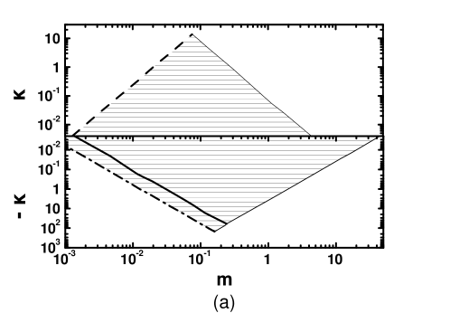
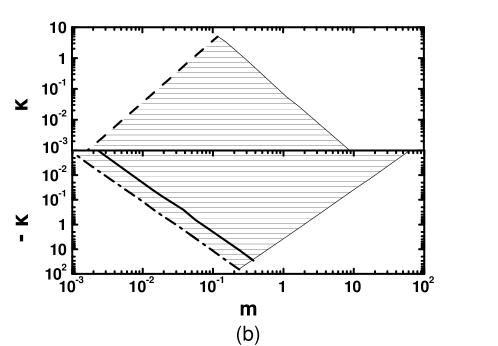
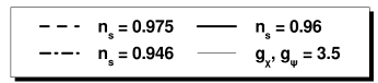
Figure 1: Allowed regions (hatched) compatible with Eqs. (20), (22), (23) and (25) in the $m-\kappa$ plane for $\Delta\widehat{V}_{\rm CI}(\phi_{\star})=0$ (a) or $\Delta\widehat{V}_{\rm CI}(\phi_{\rm f})=0$ (b). The conventions adopted for the various lines are also shown.

Varying $m$ and $\kappa$ we specify in Fig. 1 the available parameter space from the constraints of Sec. 2.3 of the model for $\Lambda$ such that $\Delta\widehat{V}_{\rm CI}(\phi_{\star})=0$ (${\sf\footnotesize a}$) or $\Delta\widehat{V}_{\rm CI}(\phi_{\rm f})=0$ (${\sf\footnotesize b}$). The conventions adopted for the various lines are also shown. In particular, the dashed [dot-dashed] lines correspond to $n_{\rm s}=0.975$ [$n_{\rm s}=0.946$], whereas the solid lines are obtained by fixing $n_{\rm s}=0.96$ – see Eq. (23). Along the thin lines $g_{\chi}$ ($\kappa>0$) or $g_{\psi}$ ($\kappa<0$) saturate their perturbative limit of $\sqrt{4\pi}\simeq 3.54$. Obviously, for $\Delta\widehat{V}_{\rm CI}(\phi_{\star})=0$ [$\Delta\widehat{V}_{\rm CI}(\phi_{\rm f})=0$] the allowed region is extended to roughly larger [lower] $\kappa$’s. Focusing on $n_{\rm s}\simeq 0.96$ with $\phi_{\star}\simeq(0.003-1)$ or $|\widehat{\phi}_{\star}|\simeq(0-7)$ and $\widehat{N}_{\star}\simeq(54.4-54.8)$ we find

$$0.017\lesssim{g_{\psi}}\lesssim 3.5,~{}0.011\lesssim{m/0.1}\lesssim 2.4~{}~{}~{}\mbox{and}~{}~{}~{}77\lesssim c_{\cal R}\lesssim 1.6\cdot 10^{4} \mbox{for}~{}~{}~{}\Delta\widehat{V}_{\rm CI}(\phi_{\star})=0,$$ (43a)

$$0.010\lesssim{g_{\psi}}\lesssim 3.5,~{}0.010\lesssim{m/0.1}\lesssim 3.5~{}~{}~{}\mbox{and}~{}~{}~{}77\lesssim c_{\cal R}\lesssim 2.5\cdot 10^{4} \mbox{for}~{}~{}~{}\Delta\widehat{V}_{\rm CI}(\phi_{\rm f})=0.~{}~{}~{}~{}~{}~{}~{}~{}~{}~{}~{}~{}~{}~{}$$ (43b)

In both cases $r\simeq 0.003$ and $\widehat{m}_{\rm\delta\phi}\simeq 1.2\cdot 10^{-5}$. Letting $n_{\rm s}$ vary within the range of Eq. (23a) we obtain $r\simeq(2.4-4.5)\cdot 10^{-3}$ and $\widehat{m}_{\rm\delta\phi}\simeq(1-1.4)\cdot 10^{-5}$.

Recapitulating this section, we could conclude that the presence of a large linear non-minimal coupling to gravity by itself or in conjunction with RCs in the inflationary potential leads to acceptable results for the observables obtained in the context of a non-SUSY quadratic inflationary model. The resulting $r$, though, is well below the sensitivity of the present experiments [4, 12].

4 Inflation in SUGRA

In this section we move on to the analysis of our SUGRA realizations of nMI. Namely, in Sec. 4.1 we extract the inflationary potential for any $n$, and we then present our results for the two radically different cases: taking $n=0$ in Sec. 4.2 and $n<0$ in Sec. 4.3.

4.1 Inflationary Potential

The (tree level) inflationary potential, $\widehat{V}_{\rm CI0}$, is obtained by applying Eq. (8b) for $z^{\alpha}=\Phi,S$ and $W,K$ given in Eqs. (9) and (17). If we express $\Phi$ and $S$ according to the standard parametrization

$$\Phi=\>{\phi\,e^{i{\theta}}}/{\sqrt{2}}\>\>\>\mbox{and}\>\>\>S=\>(s+i\bar{s})/\sqrt{2}\,,$$ (44)

and confine ourselves along the inflationary track, i.e., for

$${\theta}=s=\bar{s}=0,$$ (45)

we find that the only surviving term is

$$\widehat{V}_{\rm CI0}=\widehat{V}({\theta}=s=\bar{s}=0)=e^{K}K^{SS^{*}}\,|W_{,S}|^{2}=\frac{m^{2}|\Phi|^{2}}{2f_{S\Phi}f_{\cal R}^{2+3n}}\,,$$ (46a)

where we take into account that

$$e^{K}=f_{\cal R}^{-3(1+n)}\>\>\>\mbox{and}\>\>\>K^{SS^{*}}={f_{\cal R}/f_{S\Phi}}.$$ (46b)

Calculating $$f_{\cal R} f_{S\Phi}$$ and through the expressions

$$f_{\cal R}=1+c_{\cal R}{\phi}-{k_{\sf NS}\phi^{2}-k_{\Phi}\phi^{4}\over 6(1+n)}\>\>\>\mbox{and}\>\>\>f_{S\Phi}=\Omega_{,SS^{*}}=1-k_{S\Phi}\phi\,,$$ (46c)

and plugging them into Eq. (46a), we find that $\widehat{V}_{\rm CI0}$ takes the form

$$\widehat{V}_{\rm CI0}=\frac{m^{2}\phi^{2}}{2f_{S\Phi}f_{\cal R}^{2+3n}}\simeq\frac{m^{2}\phi^{2}}{2f_{S\Phi}}\left(1+c_{\cal R}\phi\right)^{-(2+3n)}\simeq\frac{m^{2}\phi^{-3n}}{2f_{S\Phi}c_{\cal R}^{2+3n}}\,.$$ (47)

The corresponding EF Hubble parameter is

$$\widehat{H}_{\rm CI}={\widehat{V}_{\rm CI0}^{1/2}/\sqrt{3}}\simeq{m\phi^{-3n/2}/\sqrt{6f_{S\Phi}}c_{\cal R}^{1+3n/2}}\,.$$ (48)

Given that $f_{S\Phi}\ll f_{\cal R}$ with $c_{\cal R}\gg 1$, $\widehat{V}_{\rm CI0}$ in Eq. (46a) is roughly proportional to $\phi^{-3n}$. Besides the inflationary plateau which emerges for $n=0$ and was studied in Ref. [16], a chaotic-type potential (bounded from below) is also generated for $n<0$.

The kinetic terms for the various scalars in Eq. (8a) can be brought into the following form

$$K_{{\alpha}{\bar{\beta}}}\dot{z}^{\alpha}\dot{z}^{*{\bar{\beta}}}=\frac{1}{2}\left(\dot{\widehat{\phi}}^{2}+\dot{\widehat{\theta}}^{2}\right)+\frac{1}{2}\left(\dot{\widehat{s}}^{2}+\dot{\widehat{\overline{s}}}^{2}\right)\,.$$ (49a)

Here the dot denotes derivation w.r.t the JF cosmic time and the hatted fields read

$${d\widehat{}\phi\over d\phi}=\sqrt{K_{\Phi\Phi^{*}}}=J\simeq{\sqrt{3(1+n)}\over\sqrt{2}\phi},\>\>\>\widehat{{\theta}}=J\,{\theta}\phi\>\>\>\mbox{and}\>\>\>(\widehat{s},\widehat{\bar{s}})=\sqrt{K_{SS^{*}}}{(s,\bar{s})}\,,$$ (49b)

where $K_{SS^{*}}=f_{S\Phi}/f_{\cal R}\simeq 1/c_{\cal R}\phi$ – cf. Eq. (46b). The spinors $\psi_{\Phi}$ and $\psi_{S}$ associated with $S$ and $\Phi$ are normalized similarly, i.e., $\widehat{\psi}_{S}=\sqrt{K_{SS^{*}}}\psi_{S}$ and $\widehat{\psi}_{\Phi}=\sqrt{K_{\Phi\Phi^{*}}}\psi_{\Phi}$. Integrating the first equation in Eq. (49b), we can identify the EF field as

$$\widehat{\phi}=\sqrt{3(1+n)/2}\ln\phi~{}~{}\Rightarrow~{}~{}\phi=e^{\sqrt{2/3(1+n)}\widehat{\phi}},$$ (50)

and derive $\widehat{V}_{\rm CI0}$ as a function of $\widehat{\phi}$, i.e.

$$\widehat{V}_{\rm CI0}\simeq{m^{2}e^{-\sqrt{6/(1+n)}n\widehat{\phi}}}/{2f_{S\Phi}c_{\cal R}^{2+3n}}\,.$$ (51)

From the last expression we can easily infer that, for $n\neq 0$, $\widehat{V}_{\rm CI0}$ declines away from the so-called $\alpha$-attractor models [43] which are tied to deviations from the conventional ($-3$) coefficient of the logarithm in the Kähler potential, and the resulting inflationary potential has the form $V_{0}(1-e^{-\sqrt{2/3(1+n)}\widehat{\phi}})^{2}$.

Fields	Eingestates	Masses Squared
$1$ real scalar	$\widehat{{\theta}}$	$\widehat{m}^{2}_{{\theta}}\simeq m^{2}c_{\cal R}(2+3n)\phi^{3}/3(1+n)f_{\cal R}^{3(1+n)}\simeq 4{\widehat{H}}_{\rm CI}^{2}$
$2$ real scalars	$\widehat{s},~{}\widehat{\bar{s}}$	$\widehat{m}^{2}_{s}=m^{2}\phi\left(4-c_{\cal R}\phi\left(12n+c_{\cal R}(2-9n^{2}-24k_{S}(1+n)\right)\phi\right.$
		$\left.+24c_{\cal R}^{2}k_{S}(1+n)\phi^{2})\right)/6(1+n)c_{\cal R}f_{\cal R}^{3(1+n)}$
$2$ Weyl spinors	$\widehat{\psi}_{\pm}={\widehat{\psi}_{\Phi}\pm\widehat{\psi}_{S}\over\sqrt{2}}$	$\widehat{m}^{2}_{\psi\pm}\simeq m^{2}(2-3c_{\cal R}n\phi)^{2}/6(1+n)c_{\cal R}^{2}f_{\cal R}^{(2+3n)}$

Table 2: Mass spectrum along the trajectory in Eq. (45).

The stability of the configuration in Eq. (45) can be checked by verifying the validity of the conditions

$$\left.{\partial\widehat{V}\over\partial\widehat{\chi}^{\alpha}}\right|_{\mbox{Eq.~{}(\ref{inftr})}}=0\>\>\>\mbox{and}\>\>\>\widehat{m}^{2}_{\chi^{\alpha}}>0\>\>\>\mbox{with}\>\>\>\chi^{\alpha}={\theta},s,\bar{s}.$$ (52a)

Here $$\widehat{m}^{2}_{\chi^{\alpha}}$$ are the eigenvalues of the mass matrix with elements

$$\widehat{M}^{2}_{{\alpha}{\beta}}=\left.{\partial^{2}\widehat{V}\over\partial\widehat{\chi}^{\alpha}\partial\widehat{\chi}^{\beta}}\right|_{\mbox{Eq.~{}(\ref{inftr})}}\mbox{with}\>\>\>\chi^{\alpha}={\theta},s,\bar{s}\,,$$ (52b)

and hat denotes the EF canonically normalized fields. Upon diagonalization of $\widehat{M}^{2}_{{\alpha}{\beta}}$ in Eq. (52b) we can construct the scalar mass spectrum of the theory along the direction in Eq. (45). Taking the limits $k_{\Phi}\rightarrow 0,k_{S\Phi}\rightarrow 0$ and $k_{\sf NS}\rightarrow 0$, we find the expressions of the relevant masses squared, arranged in Table 2, which approach rather well the quite lengthy, exact expressions taken into account in our numerical computation. As usual – cf. Ref. [25, 44] – the only dangerous eignestate of $\widehat{M}^{2}_{{\alpha}{\beta}}$ is $\widehat{m}^{2}_{{s}}$ which can become positive and heavy enough by conveniently selecting $k_{S}>0$ – see Secs. 4.2.2 and 4.3.2. Besides the stability requirement in Eq. (52a), from the derived spectrum we can numerically verify that the various masses remain greater than $\widehat{H}_{\rm CI}$ during the last $50$ e-foldings of nMI, and so any inflationary perturbations of the fields other than the inflaton are safely eliminated. Due to the large effective masses that ${\theta},s$ and $\bar{s}$ in Eq. (52b) acquire during CI, they enter a phase of oscillations about zero with decreasing amplitude. As a consequence, the $\phi$ dependence in their normalization – see Eq. (49b) – does not affect their dynamics. Moreover, we can observe that the fermionic (4) and bosonic (4) degrees of freedom are equal – here we take into account that $\widehat{\phi}$ is not perturbed.

Inserting the derived mass spectrum in the well-known Coleman-Weinberg formula [40], we find that the one-loop corrected inflationary potential is

$$\widehat{V}_{\rm CI}=\widehat{V}_{\rm CI0}+\Delta\widehat{V}_{\rm CI}\>\>\>\mbox{with}\>\>\>\Delta\widehat{V}_{\rm CI}={1\over 64\pi^{2}}\left(\widehat{m}_{{\theta}}^{4}\ln{\widehat{m}_{{\theta}}^{2}\over\Lambda^{2}}+2\widehat{m}_{s}^{4}\ln{\widehat{m}_{s}^{2}\over\Lambda^{2}}-4\widehat{m}_{\psi_{\pm}}^{4}\ln{\widehat{m}_{\psi_{\pm}}^{2}\over\Lambda^{2}}\right),$$ (53)

where $\Lambda$ is a renormalization group mass scale, $\widehat{m}_{{\theta}}$ and $\widehat{m}_{s}=\widehat{m}_{\bar{s}}$ are defined in Eq. (52a) and $\widehat{m}_{\psi_{\pm}}$ are the mass eigenvalues which correspond to the fermion eigenstates $\widehat{\psi}_{\pm}\simeq(\widehat{\psi}_{S}\pm\widehat{\psi}_{\Phi})/\sqrt{2}$. Following the strategy adopted in Sec. 3, we determine $\Lambda$ by requiring $\Delta\widehat{V}_{\rm CI}(\phi_{\star})=0$ or $\Delta\widehat{V}_{\rm CI}(\phi_{\rm f})=0$. Contrary to that case, though, we ignore here possible contributions to $\Delta V$ from couplings of the inflaton to the lighter degrees of freedom for two main reasons. First, these couplings are model dependent – i.e. they could be non-renormalizable (and so suppressed); second, in the SUSY framework there are almost identical contributions to $\Delta\widehat{V}_{\rm CI}$ from bosonic and fermionic degrees of freedom which cancel each other out – see Ref. [44]. As a consequence, the possible dependence of our results on the choice of $\Lambda$ can be totally avoided if we confine ourselves to $k_{S}\sim 0.5$ for $n=0$ or $k_{S}\sim 0.1$ for $n<0$ resulting to $\Lambda\simeq(2-3)\cdot 10^{14}~{}{\mbox{\rm GeV}}$ and $\Lambda\simeq(2-9)\cdot 10^{15}~{}{\mbox{\rm GeV}}$ respectively – see Secs. 4.2.2 and 4.3.2. Under these circumstances, our results can be exclusively reproduced by using $\widehat{V}_{\rm CI0}$.

The structure of $\widehat{V}_{\rm CI}$ as a function of $\phi$ for various $n$’s is displayed in Fig. 2, where we depict $\widehat{V}_{\rm CI}$ versus $\phi$ imposing $\phi_{\star}=1$. The selected values of $m,k_{S\Phi}$ and $n$, shown in Fig. 2, yield $n_{\rm s}=0.96$ and $r=0.0048,0.047,0.11$ for increasing $|n|$’s – light gray, black and gray line. The corresponding $c_{\cal R}$ values are $(0.77,7.8,38.5)\cdot 10^{2}$. We remark that a gap of about one order of magnitude emerges between $\widehat{V}_{\rm CI0}(\phi_{\star})$ for $|n|$ of order $0.01$ and $n=0$ thanks to the larger $m$ and $c_{\cal R}$ values; actually, in the former case, $\widehat{V}_{\rm CI0}^{1/4}(\phi_{\star})$ approaches the SUSY grand-unification scale, $8.2\cdot 10^{-3}$, which is imperative – see, e.g., Ref. [46] – for achieving $r$ of order $0.1$. We also observe that $\widehat{V}_{\rm CI0}$ close to $\phi=\phi_{\star}$ for $n<0$ acquires a steeper slope which is expected to have an imprint in elevating $\widehat{\epsilon}$ – see Sec. 4.3 – and, via Eq. (24c), on $r$.

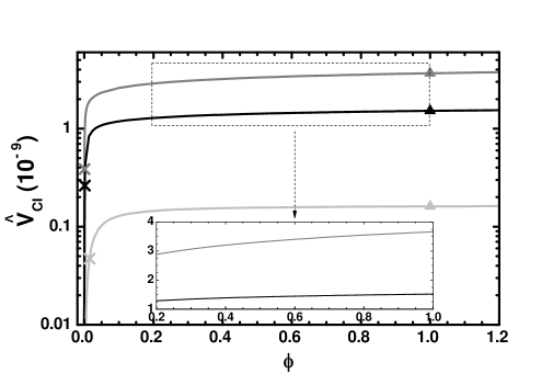
Figure 2: Inflationary potential $\widehat{V}_{\rm CI}$ (light gray, black and gray line) as a function of $\phi$ for $\phi\geq 0$, $n=0,-1/30,-1/20$, $m=0.0013,0.03,0.18$ and $k_{S\Phi}\simeq 0.0031,-0.0052,-0.0045$. Values corresponding to $\phi_{\star}$ and $\phi_{\rm f}$ are also depicted.

4.2 $n=0$ Case

We focus first on the form of Kähler potential induced by Eq. (17) with $n=0$. Our analysis in Sec. 4.2.1 presents some approximate expressions which assist us to interpret the numerical results exhibited in Sec. 4.2.2.

4.2.1 Analytic Results.

Upon substitution of Eqs. (47) and (49b) into Eq. (21b), we can extract the slow-roll parameters during the inflationary stage. Namely, we find

$$\widehat{\epsilon}=\frac{4}{3}\left(\frac{1}{c_{\cal R}\phi}+k_{S\Phi}\phi^{2}\right)^{2}\>\>\>\mbox{and}\>\>\>\widehat{\eta}=\frac{8-4c_{\cal R}\phi(1-2k_{S\Phi}\phi^{2}(5+c_{\cal R}\phi))}{3f_{\cal R}^{2}f_{S\Phi}^{2}}\,\cdot$$ (54)

It can be numerically verified that $\phi_{\star},\phi_{\rm f}$ and $\widehat{N}_{\star}$ do not decline a lot from their values for $k_{S\Phi}=0$. Therefore, Eq. (39) stabilizes our scheme against higher order terms in $\Omega_{\rm H}$ – see Eq. (15c) – despite the fact that Eq. (40) yields $\widehat{\phi}>1$ even for $\phi_{\star}<1$. Also, Eq. (38) can serve for our estimates below. In particular, replacing $\widehat{V}_{\rm CI0}$ from Eq. (47) and $\phi_{\star}$ from Eq. (38) in Eq. (22) we obtain

$$\sqrt{A_{\rm s}}=\frac{m\phi_{\star}\sqrt{1-k_{S\Phi}\phi_{\star}^{2}}}{8(\pi+c_{\cal R}k_{S\Phi}\pi\phi_{\star}^{3})}\>\>\Rightarrow\>\>m=\left(27c_{\cal R}^{2}+64k_{S\Phi}\widehat{N}_{\star}^{3}\right)\frac{2\pi\sqrt{A_{\rm s}}}{9\widehat{N}_{\star}c_{\cal R}},$$ (55)

which is quite similar to Eq. (41) obtained in the non-SUSY case. Inserting Eq. (38) into Eqs. (54) and (24) and expanding for $c_{\cal R}\gg 1$, we extract the following expressions for the observables

$$n_{\rm s}\simeq 1-\frac{2}{\widehat{N}_{\star}}+\frac{256}{27}\frac{k_{S\Phi}\widehat{N}_{\star}^{2}}{c_{\cal R}^{2}},\>\>\>a_{\rm s}\simeq-\frac{2}{\widehat{N}_{\star}^{2}}-\frac{640}{27}\frac{k_{S\Phi}\widehat{N}_{\star}}{c_{\cal R}^{2}}\>\>\>\mbox{and}\>\>\>r\simeq\frac{12}{\widehat{N}_{\star}^{2}}+\frac{512}{9}\frac{k_{S\Phi}\widehat{N}_{\star}}{c_{\cal R}^{2}}\cdot$$ (56)

As in the case of Eq. (42a), the emergent depedence of the observables on $k_{S\Phi}$ is stronger for $n_{\rm s}$, since it goes as $\widehat{N}_{\star}^{2}/c_{\cal R}^{2}$, and weaker for $a_{\rm s}$ and $r$, since they go as $\widehat{N}_{\star}/c_{\cal R}^{2}$. This depedence does not exist within no-scale SUGRA since $k_{S\Phi}$ vanishes by definition – see Eq. (18).

4.2.2 Numerical Results.

The present inflationary scenario depends on the parameters:

$$m,\>c_{\cal R},\>k_{S},\>k_{S\Phi},\>k_{\Phi}\>\>\>\mbox{and}\>\>\>T_{\rm rh}\,.$$ (57)

Our results are essentially independent of $k_{S}$ values, provided that $\widehat{m}_{s}^{2}>0$ for every allowed $m$ and $c_{\cal R}$ – see Table 2. The same is also valid for $k_{\Phi}$ since the contribution from the second term in $f_{\cal R}$, Eq. (46c), is overshadowed by the strong enough first term including $c_{\cal R}\gg 1$. We therefore set $k_{S}=k_{\Phi}=0.5$. Since we do not specify the interaction of the inflaton to the light degrees of freedom, $T_{\rm rh}$ is a free parameter. We choose $T_{\rm rh}=4.1\cdot 10^{-10}$ which is a typical value encountered in similar settings – cf. Ref. [16, 45, 44]. Besides these values, in our numerical code, we use as input parameters $c_{\cal R},~{}k_{S\Phi}$ and $\phi_{\star}$. For every chosen $c_{\cal R}$, we restrict $m$ and $\phi_{\star}$ so that Eqs. (20), (22) and (25) are satisfied. In addition, by adjusting $k_{S\Phi}$ we can achieve $n_{\rm s}$ values in the range of Eq. (23). Our results are displayed in Fig. 3-(a) [Fig. 3-(b)], where we delineate the hatched regions allowed by the above restrictions in the $m-c_{\cal R}$ [$m-k_{S\Phi}$] plane. We follow the conventions adopted for the thick lines in Fig. 1. Along the solid thin line, which provides the lower bound for the regions presented in Fig. 3, the constraint of Eq. (25b) is saturated. At the other end, the allowed regions terminate along the faint dashed line where $|k_{S\Phi}|=3$, since we expect $k_{S\Phi}$ values of order unity to be natural.

From Fig. 3-(a) we see that $c_{\cal R}$ remains almost proportional to $m$ and for constant $m$, $c_{\cal R}$ increases as $n_{\rm s}$ decreases. From Fig. 3-(b) we note that $k_{S\Phi}$ takes natural (order unity) values for $1.94\lesssim m/0.01\lesssim 7.8$ or $6\gtrsim\phi_{\star}/0.1\gtrsim 0.15$. For lower $m$ or larger $\phi_{\star}$ values some degree of tuning ($\sim 0.01$) is needed since $k_{S\Phi}$ is confined close to zero for $n_{\rm s}=0.96$, whereas for larger $m$ or lower $\phi_{\star}$ values, $k_{S\Phi}$ starts increasing sharply beyond unity. More explicitly, for $n_{\rm s}=0.96$ and ${\widehat{N}}_{\star}\simeq 52$, taking $\phi_{\star}=(0.01-1)$ or $|\widehat{\phi}_{\star}|=(0-8.6)$, we find:

$$77\lesssim c_{\cal R}\lesssim 1.5\cdot 10^{5}\>\>\>\mbox{with}\>\>\>0.49\lesssim m/0.01\lesssim 11.7\>\>\>\mbox{and}\>\>\>0.0031\lesssim|k_{S\Phi}|\lesssim 3\,.$$ (58)

For this range of values, we obtain $6.8\lesssim{|a_{\rm s}|/10^{-4}}\lesssim 8.2$ and $r\simeq 3.8\cdot 10^{-3}$ which lie within the ranges of Eq. (23). On the other hand, the results within no-scale SUGRA are much more robust since the $k_{S\Phi}$ (and $k_{\Phi}$) dependence collapses – see Eq. (18). Indeed, no-scale SUGRA predicts $n_{\rm s}\simeq 0.964,~{}a_{\rm s}=-6.5\cdot 10^{-4}$ and $r=4\cdot 10^{-3}$ identically with the non-SUSY case – see columns E and F of Table 1. The same results would have been achieved, if we had considered $S$ as a nilpotent superfield [34] since the stabilization term $|S|^{4}$ would have been absent in Eq. (17) and so all the fourth order terms could be avoided.

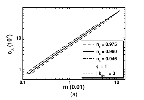
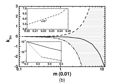
Figure 3: Allowed regions (hatched) compatible with Eqs. (20), (22), (23) and (25) in the $m-c_{\cal R}$ (a) and $m-k_{S\Phi}$ (b) plane for $n=0$ and $k_{S}=k_{\Phi}=0.5$. The conventions adopted for the various lines are shown in panel (a).

4.3 $n<0$ Case

Following the strategy of the previous section, we present below first some analytic results in Sec. 4.3.1, which provides a taste of the numerical findings exhibited in Sec. 4.3.2.

4.3.1 Analytic Results.

Plugging Eqs. (47) and (49b) into Eq. (21b), we obtain the following approximate expressions for the slow-roll parameters

$$\widehat{\epsilon}=\frac{(2-3c_{\cal R}n\phi+c_{\cal R}k_{S\Phi}(2+3n)\phi^{3})^{2}}{3(1+n)f_{\cal R}^{2}f_{S\Phi}^{2}}$$ (59a)

and

$$\widehat{\eta}=\frac{8-2c_{\cal R}\phi(2+15n-2k_{S\Phi}(10\phi^{2}+2c_{\cal R}k_{S\Phi}(2-6n)\phi^{3})}{3(1+n)f_{\cal R}^{2}f_{S\Phi}^{2}}\,\cdot$$ (59b)

Taking the limit of the expressions above for $k_{S\Phi}\simeq 0$, we can analytically solve the condition in Eq. (21a) w.r.t $\phi$. The results are

$$\phi_{1\rm f}=\frac{2}{\sqrt{3}(\sqrt{3}n+\sqrt{1+n})c_{\cal R}}\>\>\>\mbox{and}\>\>\>\phi_{2\rm f}=\frac{8}{(2+15n+\sqrt{28+84n+81n^{2}})c_{\cal R}}\cdot$$ (60)

The termination of nMI mostly occurs at $\phi_{\rm f}=\phi_{1\rm f}$ because we mainly get $\phi_{1\rm f}>\phi_{2\rm f}$.

Given that $\phi_{\rm f}\ll\phi_{\star}$ we can estimate $\widehat{N}_{\star}$ through Eq. (19),

$$\widehat{N}_{\star}=\frac{3}{2}(1+n)\left(\frac{\ln\phi_{\star}}{2}-\frac{(2+3n)\ln(2-3c_{\cal R}n\phi_{\star})}{6n}\right)\cdot$$ (61a)

Neglecting the first term in the last equality and solving w.r.t $$\phi_{\star} \phi_{\star}$$, we get an indicative value for

$$\phi_{\star}=\left(2-e_{n}\right)/3nc_{\cal R},\>\>\>\mbox{with}\>\>\>e_{n}=e^{-4n\widehat{N}_{\star}/(1+n)(2+3n)}\,.$$ (61b)

Although a radically different dependence of $$\phi_{\star} \widehat{N}_{\star} \phi_{\star} c_{\cal R}$$ on arises – cf. Eq. (38) – can again remain subplanckian for large ’s fulfilling Eq. (25b). Indeed,

$$\phi_{\star}\leq 1\>\>\>\Rightarrow\>\>\>c_{\cal R}\geq(2-e_{n})/3n\,.$$ (61c)

As in the previous cases – see Secs. 3.3 and 4.2.1 – $\widehat{\phi}$ corresponding to $\phi_{\star}$ and $\phi_{\rm f}$ turn out to be transplanckian, since plugging Eqs. (61b) and (60) into Eq. (50) we find

$$\widehat{\phi}_{\star}\simeq\sqrt{3(1+n)\over 2}\left({4|n|\widehat{N}_{\star}\over(1+n)(2+3n)}-\ln 3|n|c_{\cal R}\right)\>\>\>\mbox{and}\>\>\>\widehat{\phi}_{\rm f}\simeq\sqrt{3(1+n)\over 2}\ln{2/\sqrt{3}\over(\sqrt{3}n+\sqrt{1+n})c_{\cal R}}\,,$$ (62)

which give $|\widehat{\phi}_{\star}|\simeq(0.5-4)$ and $|\widehat{\phi}_{\rm f}|\simeq(7.7-13.4)$ for $n=-(0.03-0.05)$ – in rather good agreement with the numerical results which yield $|\widehat{\phi}_{\star}|\simeq(0-3.8)$ and identical results for $|\widehat{\phi}_{\rm f}|$. Despite this fact, our construction remains stable since the dangerous higher order terms are exclusively expressed as functions of the initial field $\Phi$, and remain harmless for $|\Phi|\leq 1$.

Upon substitution of Eq. (61b) into Eq. (22) we end up with

$$m\simeq\frac{4\sqrt{A_{\rm s}}\pi(1+(2-e_{n})/3n)^{3n/2}(27n^{3}e_{n}c_{\cal R}^{2}-k_{S\Phi}(2+3n)(e_{n}-2)^{3})}{3n\sqrt{1+n}(e_{n}-2)\sqrt{9n^{2}c_{\cal R}^{2}-k_{S\Phi}(e_{n}-2)^{2}}}\cdot$$ (63)

We remark that $m$ remains almost proportional to $c_{\cal R}$ – cf.  Eq. (55) – but it also depends both on $k_{S\Phi}$ and $n$. Inserting Eq. (61b) into Eqs. (59a) and (59b), then employing Eq. (24a) and expanding for $c_{\cal R}\gg 1$, we find

$$n_{\rm s}=1-2n\frac{8-4e_{n}+3n(4+e_{n}(e_{n}-2))}{(1+n)(e_{n}-3n-2)^{2}}+\frac{8k_{S\Phi}(2+3n)(e_{n}-2)^{3}}{27n^{2}(1+n)(e_{n}-3n-2)c_{\cal R}^{2}}\cdot$$ (64a)

Following the same steps, from Eq. (24c) we find

$$r=16\left(\frac{3n^{2}e_{n}^{2}}{(1+n)(e_{n}-3n-2)^{2}}-4k_{S\Phi}\frac{(e_{n}-2)^{2}e_{n}}{9n(1+n)(e_{n}-3n-2)c_{\cal R}^{2}}\right)\cdot$$ (64b)

From the above expressions we see that primarily $|n|\neq 0$ and secondarily $n<0$ help to reduce $n_{\rm s}$ below unity and sizably increase $r$. On the other hand, the dependence of $r$ on $k_{S\Phi}$ is rather weak since the dominant contribution originates from the first term, which is independent of $k_{S\Phi}$ and $c_{\cal R}$, whereas the correction from the second term is suppressed by an inverse power of $c_{\cal R}^{2}$. On the contrary, the depedence of $n_{\rm s}$ on $k_{S\Phi}<0$ is somehow stronger since the presence of $c_{\cal R}^{2}\gg 1$ in the denominator of the second term is accompanied by the factor $n^{2}\ll 1$, which compensates for the reduction of the corresponding contribution.

4.3.2 Numerical Results.

Besides the free parameters shown in Eq. (57) we also have $n$ which is constrained to negative values. Using the reasoning explained in Sec. 4.2.2 we set $k_{\Phi}=0.5$ and $T_{\rm rh}=4.1\cdot 10^{-10}$. On the other hand, $\widehat{m}_{s}^{2}$ can become positive with $k_{S}$ lower than the value used in Sec. 4.2.2 since positive contributions from $n<0$ arises here – see Table 2. Moreover, if $k_{S}$ takes a value of order unity $\widehat{m}_{s}^{2}$ grows more efficiently than in the case with $n=0$, rendering thereby the RCs in Eq. (53) sizeable for very large $c_{\cal R}$ values ($\sim 10^{5}$). To avoid such dependence of the model predictions on the RCs, we use $k_{S}$ values to lower than those used in Sec. 4.2.2. Thus, we set $k_{S}=0.1$ throughout. As in the previous case, Eqs. (20), (22) and (25) assist us to restrict $m$ (or $c_{\cal R}\geq 1$) and $\phi_{\star}$. By adjusting $n$ and $k_{S\Phi}$ we can achieve not only $n_{\rm s},a_{\rm s}$ and $r$ values in the range of Eq. (23) but also $r$ values in the observable region $(0.01-0.1)$.

Confronting the parameters with Eqs. (20), (22), (23a, b) and (25) we depict the allowed (hatched) regions in the $m-c_{\cal R}$, $m-k_{S\Phi}$, $m-r$ and $m-a_{\rm s}$ planes for $n=-1/30$ (light gray lines and horizontally hatched regions), $n=-1/25$ (black lines and horizontally hatched regions), $n=-1/20$ (gray lines and vertically hatched regions) in Fig. 4-(a), (b), (c) and (d) respectively. In the horizontally hatched regions $r$ is compatible with Eq. (23c), whereas in the vertically hatched region $r$ overpasses slightly this bound for $n_{\rm s}\gtrsim 0.946$. Note that the conventions adopted for the various lines are identical with those used in Fig. 3 – i.e., the dashed, solid (thick) and dot-dashed lines correspond to $n_{\rm s}=0.975,0.96$ and $0.946$ respectively, whereas along the thin (solid) lines the constraint of Eq. (25b) is saturated. The bound $|k_{S\Phi}|=3$ limits the various regions at the other end along the thin dashed line

From Fig. 4-(a) we remark that $c_{\cal R}$ remains almost proportional to $m$ but the dependence on $k_{S\Phi}$ is weaker than that shown in Fig. 3-(a). Also, as $|n|$ increases, the allowed areas are displaced to larger $m$ and $c_{\cal R}$ values in agreement with Eq. (61c) – cf. Fig. 3. Similarly, the allowed $k_{S\Phi}$ values move to the right for increasing $m$ values and fixed $n_{\rm s}$ as shown in Fig. 4-(b). Indeed, if we increase $c_{\cal R}$, Eq. (64a) dictates an increase of $k_{S\Phi}$ in order to keep $n_{\rm s}$ constant. This effect deviates somewhat from our findings in the similar settings of Ref. [25]. Finally, from Fig. 4-(c) and (d) we conclude that employing $|n|\gtrsim 0.01$, $r$ and $a_{\rm s}$ increase w.r.t their values for $n=0$ – see results below Eq. (58). As a consequence, for $n=-0.033$ and $-0.04$, $r$ enters the observable region. An increase in $r$ even larger than the present bound in Eq. (23c) is also possible. On the other hand, $a_{\rm s}$ although one order larger than its value for $n=0$ remains sufficiently low; it is thus consistent with the fitting of data with the standard $\Lambda$CDM model – see Eq. (23). As anticipated below Eq. (64b), the resulting $r$ values depend only on the input $n$ and $k_{S\Phi}$ (or $n_{\rm s}$), and are independent of $m$ (or $c_{\cal R}$). The same behavior is also true for $a_{\rm s}$. It is worth noticing that a decrease of $k_{S\Phi}$ below zero is imperative in order to simultaneous fulfill Eqs. (23a) and (c). Indeed, had we increased the prefactor $(-3)$ in Eq. (17) by eliminating the fourth order terms – by assuming, e.g., that $S$ is a nilpotent superfield [34] – the enhancement of $r$ would be accompanied with an increase of $n_{\rm s}$ which would have become incompatible with Eq. (23a).

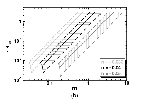
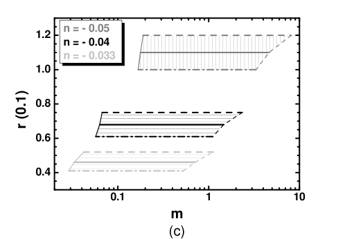
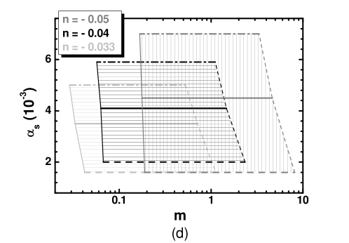
Figure 4: Allowed regions (hatched) compatible with Eqs. (20), (22), (23a, b) and (25) in the $m-c_{\cal R}$ (a), $m-k_{S\Phi}$ (b), $m-r$ (c), $m-a_{\rm s}$ (d) plane for $k_{S}=0.1$, $k_{\Phi}=0.5$ and $n=-0.033$ (light gray lines and hatched regions), $n=-0.04$ (black lines and hatched regions), $n=-0.05$ (gray lines and hatched regions). The conventions adopted for the type and color of the various lines are shown in panel (a).

More explicitly, for $n_{\rm s}=0.96$ and ${\widehat{N}}_{\star}\simeq 51.7$ we find:

$$0.78\lesssim{c_{\cal R}/10^{3}}\lesssim 18\>\>\>\mbox{with}\>\>\>0.03\lesssim m\lesssim 0.71\>\>\>\mbox{and}\>\>\>0.005\lesssim-{k_{S\Phi}}\lesssim 3\,\>\>\>(n=-0.033);\>\>\>\>\>\>$$ (65a)

$$1.45\lesssim{c_{\cal R}/10^{3}}\lesssim 34\>\>\>\mbox{with}\>\>\>0.06\lesssim m\lesssim 1.47\>\>\>\mbox{and}\>\>\>0.002\lesssim-{k_{S\Phi}}\lesssim 3\,\>\>\>(n=-0.04);\>\>\>\>\>\>\>\>\>\>\>\>\>$$ (65b)

$$3.85\lesssim{c_{\cal R}/10^{3}}\lesssim 10^{2}\>\>\>\mbox{with}\>\>\>0.18\lesssim m\lesssim 4.64\>\>\>\mbox{and}\>\>\>0.0045\lesssim-{k_{S\Phi}}\lesssim 3\,\>\>\>(n=-0.05).\>\>\>\>\>\>\>\>\>\>\>\>\>$$ (65c)

In these regions, $\phi_{\star}$ ranges from $1$ to about $0.04$ and the remaining observables are

$${r\over 0.1}=0.46,0.68,1.1\>\>\>\mbox{and}\>\>\>{a_{\rm s}\over 0.001}=3.6,4,4.5\>\>\>\mbox{for}\>\>\>-{n\over 0.01}=3.3,4,5$$ (66)

respectively. As in the similar model of Ref. [25], the observable $r$ values above are achieved with subplanckian $\phi$ values. Note that this requirement sets strict upper bound on $r$ [46, 47] – e.g., in the case of SUSY hybrid inflation [48] we have $r\leq 0.01$. However, in our present set-up, $\phi$ does not coincide with the EF inflaton, $\widehat{\phi}$, which remains transplanckian and close to the values shown in Eq. (62). Thus, our results do not contradict the Lyth bound [49], which applies to $\widehat{\phi}$.

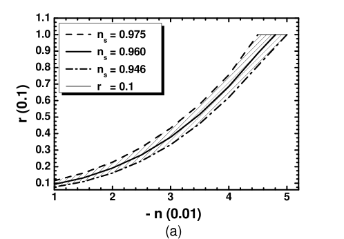
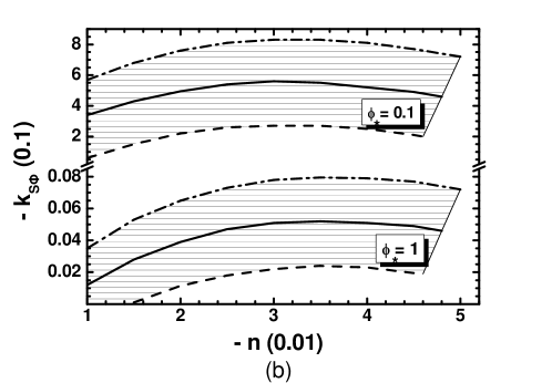
Figure 5: Allowed regions (hatched) compatible with Eqs. (20), (22), (23a, b, c) and (25) in the $(-n)-r$ plane (a) and $(-n)-(-k_{S\Phi})$ plane for $\phi_{\star}=0.1$ and $1$ (b). In both panels we set $k_{S}=0.1$ and $k_{\Phi}=0.5$. The conventions adopted for the various lines are shown in panel (a).

Taking advantage of the independence of $r$ on $m$ and $c_{\cal R}$, highlighted in Fig. 4-(c), we can delineate the allowed region of our model using $n$ as a free parameter. More specifically, fixing $\phi_{\star}$ and $n_{\rm s}$, we can vary $n$ below zero to obtain a continuous variation of the derived $r$. This way we construct the (hatched) regions allowed by all the constraints of Sec. 2.3 in the $(-n)-r$ plane – see Fig. 5-(a). We see that confining $|n|$ in the range $(0.01-0.05)$ comfortably assures observable $r$ values for any $n_{\rm s}$ in the range of Eq. (23a). We use the same shape code for the the various thick lines as in Fig. 3 and 4, whereas along the thin line here Eq. (23c) is saturated. In Fig. 5-(b) we display the allowed regions in the $(-n)-(-k_{S\Phi})$ plane for $\phi_{\star}=0.1$ (upper island) and $1$ (lower island). In all, for $n_{\rm s}=0.96,r=(0.01-0.1)$ and ${\widehat{N}}_{\star}\simeq 51.7$ we take:

$$1.32\lesssim{c_{\cal R}\over 10^{2}}\lesssim 31\>\>\>\mbox{with}\>\>\>0.03\lesssim m/0.1\lesssim 1.4\>\>\>\mbox{and}\>\>\>1.2\lesssim-{k_{S\Phi}/0.001}\lesssim 4.6\,\>\>\>(\phi_{\star}=1);\>\>\>\>\>\>\>\>\>\>\>$$ (67a)

$$1.32\lesssim{c_{\cal R}\over 10^{3}}\lesssim 31\>\>\>\mbox{with}\>\>\>0.03\lesssim m\lesssim 1.42\>\>\>\mbox{and}\>\>\>3.4\lesssim-{k_{S\Phi}/0.1}\lesssim 4.6\,\>\>\>(\phi_{\star}=0.1);\>\>\>\>\>$$ (67b)

From these results we infer that $k_{S\Phi}$ takes more natural (order one) values for lower $\phi_{\star}$ values. In fact, from Eq. (61b) we deduce that $\phi_{\star}$ decreases as $c_{\cal R}$ increases and Eq. (64a) entails an augmentation of $k_{S\Phi}$ in order the $n_{\rm s}$ value to be kept unchanged.

5 Effective Cut-off Scale

An outstanding trademark of nMI with linear coupling to gravity is that it is unitarity-safe, despite the fact that its implementation with subplanckian $\phi$ values – see Eqs. (39) and (61c) – requires relatively large $c_{\cal R}$ values. To show that this fact – first noticed in Ref. [30] – is valid for all our models we extract below the UV cut-off scale, $\Lambda_{\rm UV}$, expanding the action in Eq. (1) in the JF – see Sec. 5.1 – or this in Eq. (4) in the EF – see Sec. 5.2. Although the expansions about $\langle{\phi}\rangle=0$, presented below, are not valid [29] during nMI, we consider the $\Lambda_{\rm UV}$ extracted this way as the overall cut-off scale of the theory, since the reheating phase – realized via oscillations about $\langle{\phi}\rangle$ – is an unavoidable stage of the inflationary dynamics.

5.1 Jordan Frame Computation

Thanks to the special dependence of $f_{\cal R}$ on $\phi$ there is no interaction between the excitation of $\phi$ about $\langle{\phi}\rangle=0$, $\delta\phi$, and the graviton, $h^{\mu\nu}$ which can jeopardize the validity of perturbative unitarity. Indeed, expanding $g_{\mu\nu}$ about the flat spacetime metric $\eta_{\mu\nu}$ and the inflaton $\phi$ about its v.e.v,

$$g_{\mu\nu}\simeq\eta_{\mu\nu}+h_{\mu\nu}\>\>\>\mbox{and}\>\>\>\phi=0+\delta\phi\,,$$ (68)

and retaining only the terms with two derivatives of the excitations, the part of the lagrangian corresponding to the two first terms in the right-hand side of Eq. (4) takes the form [29, 25]

$$\delta{\cal L} = -{\langle{f_{\cal R}}\rangle\over 8}{F}_{\rm EH}\left(h^{\mu\nu}\right)+\frac{1}{2}\langle{F_{\rm K}}\rangle\partial_{\mu}\delta\phi\partial^{\mu}\delta\phi+\frac{1}{2}F_{\cal R}\left(\langle{f_{\cal R,\phi}}\rangle\delta\phi+\frac{1}{2}\langle{f_{\cal R,\phi\phi}}\rangle\delta\phi^{2}\right)$$ (69a)

$$= -{1\over 8}F_{\rm EH}\left(\bar{h}^{\mu\nu}\right)+\frac{1}{2}\partial_{\mu}\overline{}\delta\phi\partial^{\mu}\overline{}\delta\phi,$$

where $$F_{\rm K}=1 F_{\rm K}=k_{\sf NS}+3nc_{\cal R}^{2}/2 F_{\rm EH} F_{\cal R} \bar{h}_{\mu\nu} \overline{}\delta\phi$$ for the non-SUSY case and for our SUGRA scenaria; the functions and are given in Ref. [25]; and are the JF canonically normalized fields defined by the relations

$$\overline{}\delta\phi=\sqrt{\frac{\langle{f_{\cal R}}\rangle}{\langle{\bar{f}_{\cal R}}\rangle}}\delta\phi\>\>\>\mbox{and}\>\>\>\bar{h}_{\mu\nu}=\sqrt{\langle{f_{\cal R}}\rangle}\,h_{\mu\nu}+\frac{\langle{f_{\cal R,\phi}}\rangle}{\sqrt{\langle{f_{\cal R}}\rangle}}\eta_{\mu\nu}\delta\phi\>\>\>\mbox{with}\>\>\>\bar{f}_{\cal R}=F_{\rm K}f_{\cal R}+\frac{3}{2}f_{\cal R,\phi}^{2}\,,$$ (69b)

where $\langle{f_{\cal R}}\rangle=1$ and $\langle{\bar{f}_{\cal R}}\rangle=F_{\rm K}+3c_{\cal R}^{2}/2$. Since $f_{\cal R,\phi\phi}$ vanishes in the non-SUSY regime – see Eq. (7b) – and is independent on $c_{\cal R}$ in our SUSY scenario – see Eq. (46c) –, no interaction $\delta\phi^{2}h$ with $h=h^{\mu}_{\mu}$ appears – cf. Ref. [28, 29, 25] – and so the theory does not face any problem with the perturbative unitarity.

5.2 Einstein Frame Computation

Alternatively, $\Lambda_{\rm UV}$ can be determined in EF, following the systematic approach of Ref. [30]. We concentrate here on the SUGRA version of our model. The result for the non-SUSY case can be easily recovered for $n=0$ and $k_{\sf NS}=1$. Note, in passing, that the EF (canonically normalized) inflaton, in the SUGRA version is

$$\widehat{\delta\phi}=\langle{J}\rangle\delta\phi\>\>\>\mbox{with}\>\>\>\langle{J}\rangle\simeq\sqrt{3(1+n)c_{\cal R}^{2}/2+k_{\sf NS}}\,,$$ (70)

and it acquires mass given by Eq. (29). Comparing Eq. (70) with Eq. (28), we infer that the results are identical with the non-SUSY case only for the no-scale scenario. Making use of Eq. (55), we find $\widehat{m}_{\rm\delta\phi}=1.3\cdot 10^{-5}$ for the no-scale SUGRA case. Beyond no-scale SUGRA with $n=0$, replacing $m$ in Eq. (29) from Eq. (55), we find that $\widehat{m}_{\rm\delta\phi}$ inherits from $m$ a mild dependence on $k_{S\Phi}$. E.g., for $n=0$ and $n_{\rm s}$ in the range of Eq. (23a) we find $1.2\lesssim\widehat{m}_{\rm\delta\phi}/10^{-5}\lesssim 1.5$ with the lower [upper] value corresponding to the lower [upper] bound on $n_{\rm s}$ in Eq. (23). For the same $n_{\rm s}$, when $n<0$ and $r=(0.01-0.1)$ we get, using Eq. (63), $2\lesssim\widehat{m}_{\rm\delta\phi}/10^{-5}\lesssim 4$ independently of the $\phi_{\star}$ value.

The fact that $\widehat{\delta\phi}$ does not coincide with $\delta\phi$ – contrary to the standard Higgs nMI [28, 29] – ensures that our models are valid up to $M_{\rm P}$ – from now on we restore the presence of $M_{\rm P}$ in the formulas. To show it, we write the EF action ${\sf S}$ in Eq. (8a) along the path of Eq. (45) as follows

$${\sf S}=\int d^{4}x\sqrt{-\widehat{\mathfrak{g}}}\left(-\frac{1}{2}\widehat{\mathcal{R}}+\frac{1}{2}\,J^{2}\dot{\phi}^{2}-\widehat{V}_{\rm CI0}+\cdots\right),$$ (71a)

where the ellipsis represents terms irrelevant for our analysis; $$J \widehat{V}_{\rm CI0} J^{2}\dot{\phi}^{2} \langle{\phi}\rangle=0 \widehat{\delta\phi}$$ and are given by Eqs. (49b) and (47) respectively. Expanding about in terms of in Eq. (70) we arrive at the following result,

$$J^{2}\dot{\phi}^{2}=\left(1-\frac{2}{\sqrt{1+n}}\sqrt{\frac{2}{3}}\frac{\widehat{\delta\phi}}{M_{\rm P}}+\frac{2}{(1+n)}\frac{\widehat{\delta\phi}^{2}}{M_{\rm P}^{2}}-\frac{8}{3(1+n)^{3/2}}\sqrt{\frac{2}{3}}\frac{\widehat{\delta\phi}^{3}}{M_{\rm P}^{3}}+{20\over 9(1+n)^{2}}\frac{\widehat{\delta\phi}^{4}}{M_{\rm P}^{4}}-\cdots\right)\dot{}\widehat{\delta\phi}^{2}.$$ (71b)

On the other hand, $$\widehat{V}_{\rm CI0} \langle{\phi}\rangle$$ in Eq. (47) can be expanded about as follows

$$\widehat{V}_{\rm CI0}=\frac{m^{2}\widehat{\delta\phi}^{2}}{3(1+n)c_{\cal R}^{2}}\left(1-\frac{\sqrt{2}(2+3n)}{\sqrt{3(1+n)}}\frac{\widehat{\delta\phi}}{M_{\rm P}}+(2+3n)\frac{\widehat{\delta\phi}^{2}}{M_{\rm P}^{2}}-\sqrt{\frac{2}{3}}\frac{8+9n(2+n)}{3\sqrt{1+n}}\frac{\widehat{\delta\phi}^{3}}{M_{\rm P}^{3}}+\cdots\right)\cdot$$ (71c)

From the expressions above, Eqs. (71b) and (71c), we can infer that $\Lambda_{\rm UV}=M_{\rm P}$.

6 Conclusions

Inspired by the recently released Planck results [12] on the dust polarization data which appear to refute the original interpretation [4] of the Bicep2 data in terms of $r\simeq(0.16-0.2)$, we have explored quadratic CI accompanied by a strong enough linear non-minimal coupling $f_{\cal R}\gg 1$ of the inflaton to gravity. Imposing a lower bound on $c_{\cal R}$ involved in $f_{\cal R}$, we succeeded to realize nMI for subplanckian values of the inflaton, stabilizing thereby our predictions from possible higher order corrections. Moreover, in all cases, the corresponding effective theory is valid up to the Planck scale.

In the non-SUSY context we investigated ramifications to the initially proposed scenario [17] due to the presence of RCs generated by the coupling of the inflaton to matter. We showed that the RCs can affect the results on $n_{\rm s}$ but not $r$ which remains at the presently unobservable level. For $n_{\rm s}=0.96$ the model favors fermionic coupling of the inflaton with strength in the range $(0.01-3.5)$ and predicts $r\simeq 0.003$ and $\widehat{m}_{\rm\delta\phi}\simeq 3\cdot 10^{13}~{}{\mbox{\rm GeV}}$.

In the SUSY framework, we considered a superpotential with a bilinear term including two chiral superfields, which leads to the quadratic potential and can be uniquely determined by imposing an $R$ symmetry and a global $U(1)$ symmetry. On the other hand, we extended our analysis in Ref. [16] by considering a quite generic form of logarithmic Kähler potential. Namely, the prefactor multiplying the logarithm was formulated as $(-3)(1+n)$, and all possible terms up to the fourth order in powers of the various fields were considered apart from the one needed to cure the tachyonic instability, occurring along the direction of the accompanying non-inflaton field – see Eq. (17).

In the case of no-scale SUGRA, thanks to the underlying symmetries, the inflaton is not mixed with the accompanying non-inflaton field in the Kähler potential. As a consequence, the model predicts $n_{\rm s}\simeq 0.963$, $a_{\rm s}\simeq-0.00065$ and $r\simeq 0.004$, in excellent agreement with the current Planck data, and $\widehat{m}_{\rm\delta\phi}\simeq 3\cdot 10^{13}~{}{\mbox{\rm GeV}}$. Beyond no-scale SUGRA, for $n=0$, we showed that $n_{\rm s}$ spans the entire allowed range in Eq. (23a) by conveniently adjusting the coefficient $k_{S\Phi}$. In addition, for $n\simeq-(0.01-0.05)$, $r$ becomes accessible to the ongoing measurements with negligibly small $a_{\rm s}$. In this last case a mild tuning of $k_{S}$ to values of order $0.1$ is adequate so that the one-loop RCs remain subdominant and $\widehat{m}_{\rm\delta\phi}$ is confined to the range $(5-9)\cdot 10^{13}~{}{\mbox{\rm GeV}}$.

To conclude, the presence of a strong linear non-minimal coupling of the inflation to gravity can comfortably rescue CI based on the quadratic potential in both the non-SUSY and the SUSY context.

The Kähler potential used in the no-scale version of our model – see Eqs. (17) and (18) – exclusively depends on the combination

$$F_{\rm s}=\Phi+\Phi^{*},$$ (72)

which enjoys a shift symmetry w.r.t the inflaton superfield $\Phi$, according to which

$$\Phi\rightarrow\ \Phi+ic,$$ (73)

where $c$ is a real number – cf. Ref. [7]. Consequently, a tantalizing question, which should be addressed is whether CI can be realized though the imaginary part of $\Phi$, as advocated in Ref. [8] for the Starobinsky model – for another approach to the same problem see Ref. [9]. To be more specific, we check below if the combination of the superpotential in Eq. (9) with the following Kähler potential

$$K=-3(1+n)\ln\left(1+{c_{\cal R}\over\sqrt{2}}\,F_{\rm s}-{|S|^{2}+k_{\Phi}F_{\rm s}^{2}+2k_{S\Phi}|S|^{2}F_{\rm s}-\bar{k}_{S\Phi}|S|^{2}F_{\rm s}^{2}-k_{S}|S|^{4}\over 3(1+n)}\right)\,,$$ (74)

supports inflationary solutions. To analyze this possibility, we find it convenient to decompose the fields into real and imaginary parts as follows

$$\Phi=\>{(\bar{\phi}+i\phi)}/{\sqrt{2}}\>\>\>\mbox{and}\>\>\>S=\>{(\bar{s}+is)}/{\sqrt{2}}\,.$$ (75)

Thanks to the shift symmetry in Eq. (73), $K$ is independent of $\phi$ and the direction

$$\bar{\phi}=s=\bar{s}=0,$$ (76)

is a good candidate inflationary trajectory. Along it we find that $\widehat{V}$ in Eq. (8b), with $W$ and $K$ given in Eqs. (9) and (74), takes the form of the purely quadratic potential, i.e.,

$$\widehat{V}_{\rm CI0}=\widehat{V}\left(\bar{\phi}=s=\bar{s}=0\right)=\frac{1}{2}m^{2}\phi^{2}.$$ (77)

The kinetic terms of the various scalars in Eq. (8a) can be brought into the following form

$$K_{{\alpha}{\bar{\beta}}}\dot{z}^{\alpha}\dot{z}^{*{\bar{\beta}}}=\frac{1}{2}\left(\dot{\widehat{\phi}}^{2}+\dot{\widehat{\overline{\phi}}}^{2}\right)+\frac{1}{2}\left(\dot{\widehat{s}}^{2}+\dot{\widehat{\overline{s}}}^{2}\right),$$ (78a)

where the hatted fields are defined as

$${d\widehat{}\phi\over d\phi}=\sqrt{K_{\Phi\Phi^{*}}}=J=\sqrt{2k_{\Phi}+3(1+n)c_{\cal R}^{2}/2},\>\>\>\widehat{\bar{\phi}}=J\,\bar{\phi}\>\>\>\mbox{and}\>\>\>(\widehat{s},\widehat{\bar{s}})={(s,\bar{s})}.$$ (78b)

The corresponding hatted spinors are normalized similarly, i.e., $\widehat{\psi}_{S}=\psi_{S}$ and $\widehat{\psi}_{\Phi}=J\psi_{\Phi}$. However, the trajectory in Eq. (76) is not generally stable w.r.t the direction $\bar{\phi}$. This can be rectified if we impose the condition:

$$\left.\frac{\partial\widehat{V}}{\partial\widehat{\overline{\phi}}}\right|_{\mbox{Eq.~{}(\ref{inftrim})}}=-\frac{1}{2J}m^{2}\left(2\sqrt{2}k_{S\Phi}+(2+3n)c_{\cal R}\right)\phi^{2}=0~{}~{}\Rightarrow~{}~{}k_{S\Phi}=-(2+3n)c_{\cal R}/2\sqrt{2},$$ (79)

which signals a serious tuning of the parameters. In other words, the term including $k_{S\Phi}$ in Eq. (74) is imperative for the validity of this inflationary set-up. Its analysis can be realized along the lines of Sec. 2.3 using the corrected inflationary potential shown in Eq. (53) if we employ the particle spectrum displayed in Table 3. From there we note that, as in previous cases, there is an instability along the $s$ and $\bar{s}$ directions which is avoided if we set $k_{S}=1$. On the other hand, $k_{\Phi}=\bar{k}_{S\Phi}=1$ assures the positivity and heaviness of $\widehat{m}_{\bar{\phi}}^{2}$. Moreover, positive $n$ values assist us to obtain enough e-foldings of CI consistently with Eq. (25b).

Fields	Eingestates	Masses Squared
$1$ real scalar	$\widehat{\bar{\phi}}$	$\widehat{m}^{2}_{\bar{\phi}}=\left(m^{2}(6(1+n)+12\bar{k}_{S\Phi}(1+n)\phi^{2}+(2+3n)\right.$
		$\left.(4k_{\Phi}+9(1+n)^{2}c_{\cal R}^{2})\phi^{2})\right)/6(1+n)J^{2}$
$2$ real scalars	$\widehat{s},~{}\widehat{\bar{s}}$	$\widehat{m}^{2}_{s}=m^{2}\left(1/J^{2}+(6k_{S}(1+n)-1)\phi^{2}/3(1+n)\right)$
$2$ Weyl spinors	$\widehat{\psi}_{\pm}={\widehat{\psi}_{\Phi}\pm\widehat{\psi}_{S}\over\sqrt{2}}$	$\widehat{m}_{\psi\pm}=m/J$

Table 3: Mass spectrum along the trajectory in Eq. (76).

Given that the RCs remain subdominant we can approach, quite precisely, the inflationary dynamics using $\widehat{V}_{\rm CI0}$ in Eq. (77). In particular, applying Eqs. (21a) and (19) we find

$$\widehat{\epsilon}(\phi_{\rm f})=\widehat{\eta}(\phi_{\rm f})=\frac{2}{J^{2}\phi_{\rm f}^{2}}=1~{}~{}{\Rightarrow}~{}~{}\phi_{\rm f}=\frac{\sqrt{2}}{J}\>\>\>\mbox{and}\>\>\>\widehat{N}_{\star}\simeq\frac{J^{2}\phi_{\star}^{2}}{4}~{}~{}\Rightarrow~{}~{}\phi_{\star}=\frac{2}{J}\sqrt{\widehat{N}_{\star}}\,.$$ (80)

From the last equality we see that CI can be implemented with subplanckian $\phi$ values for $J\geq 2\sqrt{\widehat{N}_{\star}}$. Taking into account the normalization in Eq. (22) and employing Eq. (80) we find

$$\sqrt{A_{\rm s}}=\frac{Jm\phi_{\star}^{2}}{4\pi\sqrt{6}}~{}~{}{\Rightarrow}~{}~{}m=\frac{\sqrt{6A_{\rm s}}J\pi}{\widehat{N}_{\star}}\cdot$$ (81)

That is, contrary to the simplest quadratic CI, $m$ is not constant (for constant $\widehat{N}_{\star}$) but proportional to $J$. Upon substitution of the last expression in Eq. (80) into Eq. (24) we obtain the inflationary observables

$$n_{\rm s}=1-{2}/{\widehat{N}_{\star}}\simeq 0.962,\>\>\>a_{\rm s}=-{2}/{\widehat{N}_{\star}^{2}}\simeq 7.1\cdot 10^{-4}\>\>\>\mbox{and}\>\>\>r={8}/{\widehat{N}_{\star}}\simeq 0.15$$ (82)

for $\widehat{N}_{\star}=52.8$ corresponding to $T_{\rm rh}=4.1\cdot 10^{-10}$. As regards the mass of the inflaton at the vacuum, it can be obtained by inserting Eqs. (77) and (78b) into Eq. (29) with result

$$\widehat{m}_{\rm\delta\phi}=\sqrt{6A_{\rm s}}\pi/\widehat{N}_{\star}\simeq 6.7\cdot 10^{-6}\,.$$ (83)

Therefore, the model gives inflationary predictions identical with those of the pure quadratic CI, although with subplanckian inflaton values; thus, it is clearly in tension with the recent data [13, 11].

References

- [1] A.D. Linde, \plb1291983177.
- [2] G. Hinshaw et al. [WMAP Collaboration], Astrophys. J. Suppl. 208 19 (2013) [\arxiv1212.5226].
-
[3]
P.A.R. Ade et al. [Planck Collaboration], Astron. Astrophys. 571, A16 (2014)
[\arxiv1303.5076];
\arxiv1303.5082; http://www.esa.int/Planck. - [4] P.A.R. Ade et al. [Bicep2 Collaboration], Phys. Rev. Lett. 112, 241101 2014) [\arxiv1403.3985].
- [5] N. Okada, V.N. Şenoğuz and Q. Shafi, \arxiv1403.6403.
-
[6]
T. Kobayashi and O. Seto, Phys. Rev. D 89, 103524 (2014)
[\arxiv1403.5055];
S.M. Boucenna, S. Morisi, Q. Shafi and J.W.F. Valle, Phys. Rev. D902014055023 [\arxiv1404.3198]. -
[7]
M. Kawasaki, M. Yamaguchi and T. Yanagida,
Phys. Rev. Lett.8520003572 [\hepph0004243];
P. Brax and J. Martin, Phys. Rev. D 72 023518 (2005) [\hepth0504168];
S. Antusch, K. Dutta, P.M. Kostka, \plb6772009221 [\arxiv0902.2934];
R. Kallosh, A. Linde and T. Rube, Phys. Rev. D832011043507 [\arxiv1011.5945];
T. Li, Z. Li and D.V. Nanopoulos, J. Cosmology Astropart. Phys022014028 [\arxiv1311.6770];
K. Harigaya and T.T. Yanagida, \plb734201413 [\arxiv1403.4729];
R. Kallosh, A. Linde and A. Westphal, Phys. Rev. D902014023534 [\arxiv1405.0270];
A. Mazumdar, T. Noumi and M. Yamaguchi, Phys. Rev. D902014043519 [\arxiv1405.3959];
C. Pallis and Q. Shafi, \plb7362014261 [\arxiv1405.7645]. -
[8]
S. Ferrara, A. Kehagias and A. Riotto,
Fortsch. Phys. 62, 573 (2014) [\arxiv1403.5531];
R. Kallosh et al. J. Cosmology Astropart. Phys072014053 [\arxiv1403.7189];
K. Hamaguchi, T. Moroi and T. Terada, \plb7332014305 [\arxiv1403.7521];
S. Ferrara, A. Kehagias and A. Riotto, \arxiv1405.2353. -
[9]
J. Ellis, M. Garcia, D. Nanopoulos and
K. Olive, J. Cosmology Astropart. Phys052014037 [\arxiv1403.7518];
J. Ellis, M. Garcia, D. Nanopoulos and K. Olive, J. Cosmology Astropart. Phys082014044 [\arxiv1405.0271]. -
[10]
H. Liu, P. Mertsch and S. Sarkar, Astrophys. J. 789, L29 (2014)
[\arxiv1404.1899];
J. Martin, C. Ringeval, R. Trotta and V. Vennin, Phys. Rev. D902014063501 [\arxiv1405.7272];
R. Flauger, J.C. Hill and D.N. Spergel, J. Cosmology Astropart. Phys082014039 [\arxiv1405.7351];
M. Cortês, A.R. Liddle and D. Parkinson, \arxiv1409.6530. - [11] M.J. Mortonson and U. Seljak, J. Cosmology Astropart. Phys102014035 [\arxiv1405.5857].
- [12] R. Adam et al. [Planck Collaboration], \arxiv1409.5738.
-
[13]
C. Cheng, Q. G. Huang and S. Wang,
J. Cosmology Astropart. Phys122014044 [\arxiv1409.7025];
L. Xu, \arxiv1409.7870. - [14] V.N. Şenoğuz and Q. Shafi, \plb66820086 [\arxiv0806.2798].
- [15] K. Enqvist and M. Karčiauskas, J. Cosmology Astropart. Phys022014034 [\arxiv1312.5944].
- [16] C. Pallis and Q. Shafi, Phys. Rev. D862012023523 [\arxiv1204.0252].
- [17] C. Pallis, \plb6922010287 [\arxiv1002.4765].
- [18] R. Kallosh, A. Linde and D. Roest, Phys. Rev. Lett. 112, 011303 (2014) [\arxiv1310.3950].
- [19] C. Pallis, PoS Corfu 2012, 061 (2013) [\arxiv1307.7815].
-
[20]
F.L. Bezrukov, A. Magnin and M. Shaposhnikov, \plb675200988
[\arxiv0812.4950];
D.P. George, S. Mooij and M. Postma, J. Cosmology Astropart. Phys022014024 [\arxiv1310.2157];
J.L. Cook, L.M. Krauss, A.J. Long and S. Sabharwal, Phys. Rev. D892014103525 [\arxiv1403.4971]. -
[21]
N. Okada, M.U. Rehman and Q. Shafi, Phys. Rev. D822010043502 [\arxiv1005.5161];
N. Okada, M.U. Rehman and Q. Shafi, \plb5202011701 [\arxiv1102.4747]. -
[22]
F.R. Bouchet et al. [COrE Collaboration],
\arxiv1102.2181; http://www.core-mission.org
P. Andre et al. [PRISM Collaboration], J. Cosmology Astropart. Phys022014006 [\arxiv1310.1554]. - [23] A. Kogut et al., J. Cosmology Astropart. Phys072011025 [\arxiv1105.2044].
- [24] T. Matsumura et al., Journal of Low Temperature Physics 176, 733 (2014) [\arxiv1311.2847].
-
[25]
C. Pallis, J. Cosmology Astropart. Phys082014057
[\arxiv1403.5486];
C. Pallis, J. Cosmology Astropart. Phys102014058 [\arxiv1407.8522]. - [26] J. Tauber et al. [Planck Collaboration], \astroph0604069.
- [27] D. Baumann et al. [CMBPol Study Team Collaboration], AIP Conf. Proc. 1141, 10 (2009) [\arxiv0811.3919].
-
[28]
J.L.F. Barbon and J.R. Espinosa,
Phys. Rev. D792009081302 [\arxiv0903.0355];
C.P. Burgess, H.M. Lee and M. Trott, \jhep072010007 [\arxiv1002.2730];
M.P. Hertzberg, \jhep112010023 [\arxiv1002.2995]. -
[29]
F. Bezrukov, A. Magnin, M. Shaposhnikov and
S. Sibiryakov,
\jhep016201101 [\arxiv1008.5157]. - [30] A. Kehagias, A.M. Dizgah and A. Riotto, Phys. Rev. D892014043527 [\arxiv1312.1155].
- [31] Y. Fujii and K. Maeda, The Scalar-Tensor Theory of Gravitation (Cambridge, 2003).
-
[32]
M.B. Einhorn and D.R.T. Jones,
\jhep032010026 [\arxiv0912.2718];
H.M. Lee, J. Cosmology Astropart. Phys082010003 [\arxiv1005.2735];
S. Ferrara et al., Phys. Rev. D832011025008 [\arxiv1008.2942];
C. Pallis and N. Toumbas, J. Cosmology Astropart. Phys022011019 [\arxiv1101.0325]. - [33] S.V. Ketov and T. Terada, \arxiv1408.6524; S. Aoki and Y. Yamada, \arxiv1409.4183.
-
[34]
I. Antoniadis, E. Dudas, S. Ferrara and A. Sagnotti, Phys. Lett. B 733, 32 (2014)
[\arxiv1403.3269];
S. Ferrara, R. Kallosh and A. Linde, \arxiv1408.4096;
R. Kallosh and A. Linde, \arxiv1408.5950;
G. Dall’Agata and F. Zwirner, \arxiv1411.2605. - [35] J. Ellis, D.V. Nanopoulos and K.A. Olive, J. Cosmology Astropart. Phys102013009 [\arxiv1307.3537].
-
[36]
E. Cremmer, S. Ferrara, C. Kounnas and D.V. Nanopoulos,
Phys. Lett. B 133, 61 (1983);
J.R. Ellis, A.B. Lahanas, D.V. Nanopoulos and K. Tamvakis, Phys. Lett. B 134, 429 (1984). -
[37]
D.H. Lyth and
A. Riotto, Phys. Rept. 314, 1 (1999) [hep-ph/9807278];
G. Lazarides, J. Phys. Conf. Ser. 53, 528 (2006) [hep-ph/0607032];
A. Mazumdar and J. Rocher, Phys. Rept. 497, 85 (2011) [\arxiv1001.0993];
J. Martin, C. Ringeval and V. Vennin, Physics of the Dark Universe 5-6, 75 (2014) [\arxiv1303.3787]. - [38] C. Pallis, “High Energy Physics Research Advances”, edited by T.P. Harrison and R.N. Gonzales (Nova Science Publishers Inc., New York, 2008) [\arxiv0710.3074].
-
[39]
L. Dai, M. Kamionkowski and J. Wang,
Phys. Rev. Lett.1132014041302 [\arxiv1404.6704];
J.B. Munoz and M. Kamionkowski, \arxiv1412.0656. - [40] S.R. Coleman and E.J. Weinberg, Phys. Rev. D719731888.
-
[41]
Y. Watanabe and E. Komatsu, Phys. Rev. D752007061301
[\grqc0612120];
Y. Watanabe, Phys. Rev. D832011043511 [\arxiv1011.3348]. - [42] C. Pallis, \npb7512006129 [\hepph0510234].
-
[43]
R. Kallosh, A. Linde and D. Roest,
\jhep112013198 [\arxiv1311.0472];
R. Kallosh, A. Linde and D. Roest, \jhep082014052 [\arxiv1405.3646]. - [44] C. Pallis, J. Cosmology Astropart. Phys042014024 [\arxiv1312.3623].
- [45] C. Pallis and N. Toumbas, J. Cosmology Astropart. Phys122011002 [\arxiv1108.1771].
- [46] A. Kehagias and A. Riotto, Phys. Rev. D892014101301 [\arxiv1403.4811].
- [47] S. Antusch and D. Nolde, J. Cosmology Astropart. Phys052014035 [\arxiv1404.1821].
- [48] M. Civiletti, C. Pallis and Q. Shafi, Phys. Lett. B 733, 276 (2014) [\arxiv1402.6254].
-
[49]
D.H. Lyth, Phys. Rev. Lett.7819971861
[\hepph9606387];
R. Easther, W.H. Kinney and B.A. Powell, J. Cosmology Astropart. Phys082006004 [\astroph0601276]. - [50]