Grand Unification and Subcritical Hybrid Inflation

Abstract

We consider hybrid inflation for small couplings of the inflaton to matter such that the critical value of the inflaton field exceeds the Planck mass. It has recently been shown that inflation then continues at subcritical inflaton field values where quantum fluctuations generate an effective inflaton mass. The effective inflaton potential interpolates between a quadratic potential at small field values and a plateau at large field values. An analysis of the allowed parameter space leads to predictions for the scalar spectral index $n_{s}$ and the tensor-to-scalar ratio $r$ similar to those of natural inflation. Using the ranges for $n_{s}$ and $r$ favoured by the Planck data, we find that the energy scale of the plateau is constrained to the interval $(1.6-2.4)\times 10^{16}\,\mathrm{GeV}$, which includes the energy scale of gauge coupling unification in the supersymmetric standard model. The tensor-to-scalar ratio is predicted to satisfy the lower bound $r>0.049$ for $60$ $e$-folds before the end of inflation.

I I. introduction

The observations and analyses of the cosmic microwave background (CMB) by the WMAP Hinshaw:2012aka and Planck Ade:2013uln collaborations strongly support single-field slow-roll inflation as the paradigm of early universe cosmology. The current CMB data can be successfully described by many models of inflation. Prominent examples are the Starobinsky model Starobinsky:1980te , chaotic inflation Linde:1983gd , natural inflation Freese:1990rb and hybrid inflation Linde:1993cn , which differ significantly in their predictions for the scalar spectral index $n_{s}$ and the tensor-to-scalar ratio $r$ of the primordial density fluctuations. The recently released BICEP2 data Ade:2014xna , which are presently under intense scrutiny Mortonson:2014bja ; Flauger:2014qra ; Adam:2014bub , have renewed the interest in models with a large fraction of tensor modes.

A theoretically attractive framework is supersymmetric D-term inflation Binetruy:1996xj ; Halyo:1996pp ; Kallosh:2003ux . It is remarkable that it contains the rather different models listed above for different choices of the Kähler potential: For a canonical Kähler potential one obtains standard hybrid inflation, for a superconformal or no-scale Kähler potential the Starobinsky model emerges Buchmuller:2012ex , and in case of a shift symmetric Kähler potential Kawasaki:2000yn D-term inflation includes a “chaotic regime” with a large tensor-to-scalar ratio Buchmuller:2014rfa .

In this note we study the chaotic regime of D-term inflation in more detail. It turns out that the predictions are qualitatively similar to those of natural inflation, although the theoretical interpretation is entirely different. Moreover, there are significant quantitative differences.

The parameters of D-term inflation are a Yukawa coupling, the Fayet-Iliopoulos (FI) term and a gauge coupling. The last two determine the energy scale $M_{\rm inf}$ of hybrid inflation. The measured amplitude of scalar fluctuations determines $M_{\rm inf}$ as function of the Yukawa coupling. Imposing the bounds of the Planck data on $n_{s}$ and $r$ as constraints Ade:2013uln ,

$$\begin{split}n_{s}&=0.9603\pm 0.0073\ ,\\ r&<0.11\,(95\%\,{\rm CL})\ ,\end{split}$$ (1)

we find that $M_{\rm inf}$ has to be close to the energy scale $M_{\rm GUT}$ of grand unification. Furthermore, we obtain a lower bound on the tensor-to-scalar ratio, $r>0.049\,(0.085)$ for $60\,(50)$ $e$-folds before the end of inflation, which is in reach of upcoming experiments.

II II. Subcritical Hybrid Inflation

The framework of D-term hybrid inflation in supergravity is defined by a Kähler potential, a superpotential and a D-term scalar potential Binetruy:1996xj ; Halyo:1996pp ; Kawasaki:2000yn ; Buchmuller:2014rfa ,

$$K =\frac{1}{2}(\Phi+\Phi^{\dagger})^{2}+|S_{+}|^{2}+|S_{-}|^{2}\ ,$$ (2)

$$W =\lambda\ \Phi S_{+}S_{-}\ ,$$ (3)

$$V_{D} =\frac{g^{2}}{2}\left(|S_{+}|^{2}-|S_{-}|^{2}-\xi\right)^{2}\ .$$ (4)

The “waterfall fields” $S_{\pm}$ carry the U(1) charges $\pm 1$, and the inflaton is contained in the gauge singlet $\Phi$. The Kähler potential is invariant under the shift ${\rm Im}(\Phi)\rightarrow{\rm Im}(\Phi)+\alpha$ where $\alpha$ is a real constant, i.e., it is independent of the constant part of ${\varphi}\equiv\sqrt{2}\,{\rm Im}(\Phi)$, which is identified as the inflaton field. The gauge coupling $g=\mathcal{O}(1)$, and $\lambda$ is a Yukawa coupling, which may be much smaller than $g$. The only dimensionful parameter is the FI term $\xi$ that sets the energy scale of inflation.

Standard hybrid inflation takes place at inflaton field values $\varphi$ larger than the critical value $\varphi_{c}=(g/\lambda)\sqrt{2\xi}$. Here the waterfall fields $S_{\pm}$ have a positive mass squared and are stabilized at the origin. Classically, the potential is independent of modulus and phase of the gauge-singlet $\Phi$. The flatness in $|\Phi|$ is lifted by quantum corrections.

For subcritical field values $|\Phi|<\sqrt{2}\varphi_{c}$ the complex scalar $S_{-}$ remains stabilized at the origin, whereas $S_{+}$ acquires a tachyonic instability. The sum of F- and D-terms yields for the scalar potential as function of $\varphi$ and $s\equiv\sqrt{2}|S_{+}|$,

$$V(\varphi,s) =V_{F}(\varphi,s)+V_{D}(s)$$ (5)

$$=\frac{\lambda^{2}}{4}s^{2}\varphi^{2}+\frac{g^{2}}{8}\left(s^{2}-2\xi\right)^{2}+\mathcal{O}(s^{2n}\varphi^{2})\ ,\ n\geq 2\ .$$

Note that, due to the shift symmetry of the Kähler potential, the Planck suppressed terms are also only quadratic in $\varphi$. The scalar potential contains higher powers in ${\rm Re}(\Phi)$, which we have neglected since they are not important for inflation.

Following ref. Buchmuller:2014rfa , we solve the classical equations of motion for homogeneous fields, corresponding to the scalar potential (5),

$$\begin{split}\ddot{\varphi}+3H\dot{\varphi}+\frac{\lambda^{2}}{2}s^{2}\varphi&=0\ ,\\ \ddot{s}+3H\dot{s}-\left(g^{2}\xi-\frac{\lambda^{2}}{2}\varphi^{2}\right)s+\frac{g^{2}}{2}s^{3}&=0\ .\end{split}$$ (6)

The initial conditions for the waterfall field are obtained by considering the tachyonic growth of its quantum fluctuations Felder:2000hj ; Asaka:2001ez ; Copeland:2002ku ; Dufaux:2010cf close to the critical point $\varphi_{c}$,

$$\langle s^{2}(t)\rangle\simeq\int_{0}^{k_{b}(t)}dk\,\frac{k^{2}}{2\pi^{2}}\,e^{-3H_{c}t}\,|s_{k}(t)|^{2}\ .$$ (7)

Here $s_{k}(t)$ are the momentum modes of the field operator in an exponentially expanding, spacially flat background with Hubble parameter $H_{c}=H(\varphi_{c})$ and a time-dependent inflaton field $\varphi(t)=\varphi_{c}+\dot{\varphi}_{c}t$ Asaka:2001ez ,

$$\ddot{s}_{k}+\left(k^{2}e^{-2H_{c}t}-\frac{9}{4}H_{c}^{2}-D^{3}t\right)s_{k}=0\ .$$ (8)

The integration in eq. (7) extends over all soft momentum modes below $k_{b}(t)$ where the time-dependent mass operator for $s_{k}(t)$ in the brackets of eq. (8) vanishes. At a decoherence time $t_{\rm dec}\sim(3\ln(2R_{\rm dec})/4)^{2/3}/D$, where $R_{\rm dec}\sim 100$ and $D=(\sqrt{2\xi}g\lambda|\dot{\varphi}_{c}|)^{1/3}$, the waterfall field becomes classical. Matching the variance and classical field near the decoherence time, $s(t)\equiv\langle s^{2}(t)\rangle^{1/2}$, one obtains $s$ and $\dot{s}$ at $t=t_{\rm dec}$. As shown in ref. Buchmuller:2014rfa , the classical waterfall field reaches the local, inflaton-dependent minimum soon after the decoherence time,

$$s_{\rm min}^{2}(\varphi)=2\xi-(\lambda^{2}/g^{2})\varphi^{2}\ ,$$ (9)

and, together with the inflaton field, it reaches the global minimum after a large number of $e$-folds.

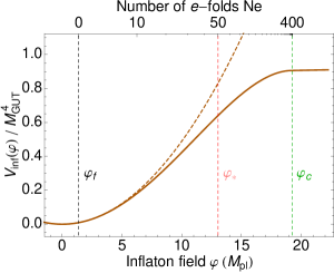
Figure 1: Effective inflaton potential in subcritical hybrid inflation (solid line) normalized to $M_{\rm GUT}^{4}$, with $M_{\rm GUT}=2\times 10^{16}\,\mathrm{GeV}$. For reference, a quadratic potential is shown (dashed line). $\varphi_{c}$, $\varphi_{*}$ and $\varphi_{f}$ are the inflaton field values at the beginning of the waterfall transition, beginning and end of the last 50 $e$-folds of inflation. Parameters: $\bar{\lambda}=7\times 10^{-4}$, $M_{\rm inf}=1.95\times 10^{16}\,\mathrm{GeV}$. (See also fig. 3 in ref. Buchmuller:2014rfa ).

On the inflationary trajectory, the inflaton potential takes a simple form,

$$V_{\rm inf}(\varphi) =V(\varphi,s_{\rm min}(\varphi))$$

$$=g^{2}\xi^{2}\ \frac{\varphi^{2}}{\varphi^{2}_{c}}\left(1-\frac{1}{2}\frac{\varphi^{2}}{\varphi^{2}_{c}}\right)\ ,\quad\varphi\leq\varphi_{c}\ .$$ (10)

For small $\varphi$, the potential is quadratic, and as $\varphi$ approaches $\varphi_{c}$, the potential reaches the plateau $g^{2}\xi^{2}/2$. Fig. 1 shows the potential for a certain choice of parameters. As we shall see in the following sections, in the relevant parameter range the predictions for $n_{s}$ and $r$ only depend on the potential (II). The initial conditions, in particular the initial value of $\varphi$ and the tachyonic growth of the waterfall field only affect the total number of $e$-folds and the formation of cosmic strings.

III III. cosmological observables

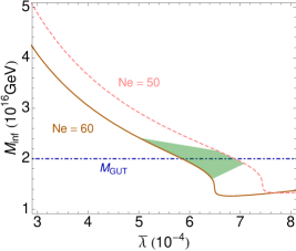
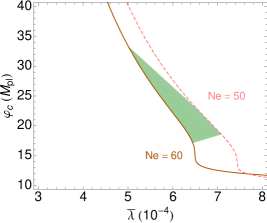
Figure 2: Lines in the $\bar{\lambda}-M_{\rm inf}$ plane (left) and the $\bar{\lambda}-\varphi_{c}$ plane (right), which are determined by the measured amplitude of the scalar power spectrum for $N_{e}=60$ and $50$. The shaded regions are allowed by the bound on $n_{s}$ and $r$ obtained from the Planck data. $M_{\rm GUT}=2\times 10^{16}\,\mathrm{GeV}$.

In this section we analyse the implications of the constraints on the cosmological observables $n_{s}$ and $r$ by the Planck data on the parameters of the inflaton potential (II). Obviously, the potential only depends on two parameters, which can be chosen as

$$M_{\rm inf}=\left(\frac{g\xi}{\sqrt{2}}\right)^{1/2}\ ,\quad\bar{\lambda}=\frac{\lambda}{\sqrt{g}}\ ,$$ (11)

where we have used $\varphi_{c}^{2}=2\sqrt{2}M_{\rm inf}^{2}/\bar{\lambda}^{2}$. Then the energy density of the plateau is given by $V_{\rm inf}(\varphi_{c})=M_{\rm inf}^{4}\,$.

Scalar spectral index and tensor-to-scalar ratio are conveniently expressed in terms of the slow-roll parameters of the inflaton potential,

$$\epsilon(\varphi)=\frac{1}{2}\left(\frac{V_{\rm inf}^{\prime}}{V_{\rm inf}}\right)^{2}\ ,\quad\eta(\varphi)=\frac{V_{\rm inf}^{\prime\prime}}{V_{\rm inf}}\ ,$$ (12)

where the superscript ‘prime’ denotes the derivative with respect to $\varphi$, and we have set the Planck mass $M_{\rm pl}=1$. Inflation ends at $\varphi=\varphi_{f}$ which is defined by ${\rm max}\{\epsilon(\varphi_{f}),\,|\eta(\varphi_{f})|\}=1$. The number of $e$-folds between $t_{*}$ and $t_{f}$ can then be expressed as

$$N_{e}=\int^{t_{f}}_{t_{*}}dt\,H=\int^{\varphi_{*}}_{\varphi_{f}}d\varphi\frac{1}{\sqrt{2\epsilon(\varphi)}}\ ,$$ (13)

where $\varphi_{*}=\varphi(t_{*})$. Solving this equation, one obtains $\varphi_{*}$ in terms of $N_{e}$,

$$\varphi_{*}^{2}=4N_{e}+2-\sum_{n\geq 1}\frac{a_{n}}{\varphi_{c}^{2n}}\ ,$$ (14)

where $a_{1}=4(N_{e}^{2}+N_{e}+1)$, $a_{2}=(2/3)(2N_{e}^{2}-3)(2N_{e}+3)$, $a_{3}=-(4/3)(N_{e}^{4}+2N_{e}^{3}+6N_{e}^{2}-3),\ldots$. The first 3 terms in the expansion (14) yield $\varphi_{*}$ to sufficient accuracy. Together with the standard expressions for $n_{s}$ and $r$,

$$n_{s}=1+2\eta_{*}-6\epsilon_{*}\ ,\quad r=16\epsilon_{*}\ ,$$ (15)

where $\epsilon_{*}=\epsilon(\varphi_{*})$ and $\eta_{*}=\eta(\varphi_{*})$, this yields $n_{s}$ and $r$ for a given number of $e$-folds $N_{e}$.

Finally, a crucial observable is the amplitude of the scalar power spectrum $A_{s}$,

$$A_{s}=\frac{V_{\rm inf}(\varphi_{*})}{24\pi^{2}\epsilon_{*}}\ ,$$ (16)

which is determined as $A_{s}=2.196^{+0.051}_{-0.060}\times 10^{-9}$ at $68$% CL Ade:2013zuv from the combined data sets of the Planck and WMAP collaborations. Imposing the central value of $A_{s}$ as constraint yields a line in the $\bar{\lambda}-M_{\rm inf}$ plane for a given number of $e$-folds. The result is shown in fig. 2 for $N_{e}=60$ and $50$. The shaded region is consistent with the constraints (1) of the Planck data on $n_{s}$ and $r$. The energy scale of the plateau is rather precisely determined,

$$1.6\ (1.9)\,\leq\left(\frac{M_{\rm inf}}{10^{16}\,{\rm GeV}}\right)\leq\,2.4\ (2.2)\ ,$$ (17)

for $N_{e}=60\,(50)$. It is very remarkable how accurately the energy scale $M_{\rm inf}$ of the plateau agrees with the energy scale $M_{\rm GUT}$ of gauge coupling unification in the supersymmetric standard model. For comparison, fig. 2 also shows the allowed region in the $\bar{\lambda}-\varphi_{c}$ plane. The allowed values of $\varphi_{c}$, and also $\varphi_{*}$ are super-Planckian, similar to chaotic inflation.

Varying $\bar{\lambda}$ yields a line also in the $r-n_{s}$ plane for a given number of $e$-folds. In fig. 3 the result is compared with various constraints from CMB data and the prediction of natural inflation Ade:2013uln . As one can see, subcritical hybrid inflation and natural inflation Freese:1990rb ; Freese:2014nla yield qualitatively similar predictions. This is not surprising, given the similarity of the potential (II) to a cosine-potential. The interpretation, however, is very different. In natural inflaton the band is obtained by varying a super-Planckian axion decay constant or, as in aligned two-axion models Kim:2004rp , the ratio of sub-Planckian decay constants. On the contrary, in subcritical hybrid inflation different points of the band correspond to different values of the ratio of a small Yukawa coupling and a gauge coupling $\mathcal{O}(1)$. The lower bound from the Planck data on the spectral index $n_{s}$ implies the lower bound on the tensor-to-scalar ratio $r>0.049\,(0.085)$ for $60\,(50)$ $e$-folds before the end of inflation.

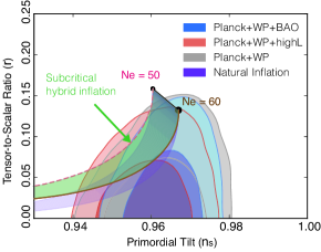
Figure 3: $68$% and $95$% CL regions in the $n_{s}-r$ plane from Planck data in combination with other data sets compared to natural inflation, as given in ref. Ade:2013uln , and subcritical hybrid inflation (green).

Let us finally comment on the formation of cosmic strings in subcritical hybrid inflation. Cosmic strings are produced during the tachyonic growth of the waterfall field, which spontaneously breaks the U(1) symmetry. The initial average distance of the cosmic strings can be estimated as Buchmuller:2014rfa

$$d_{\rm cs}(t^{\rm loc}_{\rm sp})\sim k_{b}^{-1}(t)a(t)|_{t=t^{\rm loc}_{\rm sp}}=\mathcal{O}\left(\frac{1}{H_{c}}\right)\ ,$$ (18)

where $a(t)$ is the scale factor and $t^{\rm loc}_{\rm sp}$ is the spinodal time at which $s(t)$ reaches the local, inflaton-dependent minimum $s_{\rm min}(\varphi)$. Between $t^{\rm loc}_{\rm sp}$ and $t_{*}$, the beginning of the last 50–60 $e$-folds, the scale factor grows by $\Delta N_{e}$ $e$-folds whereas the Hubble parameter remains almost constant, $H_{*}\sim H_{c}$, which yields for the average string separation at $t_{*}$,

$$d_{\rm cs}(t_{*})\sim e^{\Delta N_{e}}\frac{1}{H_{*}}\ .$$ (19)

The smallest value of $\Delta N_{e}$ is obtained for the largest coupling $\bar{\lambda}_{\rm max}=7\times 10^{-4}$: $\Delta N_{e}^{\rm min}\simeq 380$ (see figs. 1 and 2). During the final $50$–$60$ $e$-folds the horizon at $t_{*}$ is blown up to $1/H_{0}$, the size of the present universe. We thus obtain the lower bound on the average cosmic string distance

$$d_{\rm cs}(t_{0})>e^{380}\frac{1}{H_{0}}\ .$$ (20)

Hence, cosmic strings are unobservable in subcritical hybrid inflation for parameters consistent with the Planck data.

IV IV. conclusions

We have studied subcritical hybrid inflation, which occurs in supersymmetric D-term inflation for small couplings of the inflaton to matter. The effective inflaton potential interpolates between a quadratic potential at small field values and a plateau at large field values. It is characterized by two parameters, the energy scale of the plateau, and the critical value of the inflaton field, at which the plateau is reached.

The model can accommodate the Planck data very well, and it is striking how accurately the energy scale $M_{\rm inf}$ of inflation agrees with the scale $M_{\rm GUT}$ of gauge coupling unification in the supersymmetric standard model. This reopens the question on the possible connection between grand unification and inflation.

The predictions for the scalar spectral index and tensor-to-scalar ratio are qualitatively similar to those from natural inflation. Quantitatively, however, the predicted values for the tensor-to-scalar ratio are larger and one obtains the lower bounds $r>0.049\,(0.085)$ for $60\,(50)$ $e$-folds before the end of inflation, which is in reach of upcoming experiments.

Acknowledgements
We are grateful to Valerie Domcke and Kai Schmitz for valuable discussions and support. We also thank Rose Lerner, Alexander Westphal and Clemens Wieck for helpful comments on the manuscript. This work has been supported in part by the German Science Foundation (DFG) within the Collaborative Research Center 676 “Particles, Strings and the Early Universe”.

References

- (1) G. Hinshaw et al. [WMAP Collaboration], Astrophys. J. Suppl. 208 (2013) 19 [arXiv:1212.5226 [astro-ph.CO]].
- (2) P. A. R. Ade et al. [Planck Collaboration], Astron. Astrophys. 571, A22 (2014) [arXiv:1303.5082 [astro-ph.CO]].
- (3) A. A. Starobinsky, Phys. Lett. B 91 (1980) 99; Sov. Astron. Lett. 9 (1983) 302.
- (4) A. D. Linde, Phys. Lett. B 129, 177 (1983).
- (5) K. Freese, J. A. Frieman and A. V. Olinto, Phys. Rev. Lett. 65 (1990) 3233.
-
(6)
A. D. Linde,
Phys. Rev. D 49 (1994) 748
[astro-ph/9307002]. - (7) P. A. R. Ade et al. [BICEP2 Collaboration], Phys. Rev. Lett. 112, 241101 (2014) [arXiv:1403.3985 [astro-ph.CO]].
- (8) M. J. Mortonson and U. Seljak, JCAP 1410 (2014) 10, 035 [arXiv:1405.5857 [astro-ph.CO]].
- (9) R. Flauger, J. C. Hill and D. N. Spergel, JCAP 1408 (2014) 039 [arXiv:1405.7351 [astro-ph.CO]].
- (10) R. Adam et al. [Planck Collaboration], arXiv:1409.5738 [astro-ph.CO].
- (11) P. Binetruy and G. R. Dvali, Phys. Lett. B 388, 241 (1996) [hep-ph/9606342].
- (12) E. Halyo, Phys. Lett. B 387, 43 (1996) [hep-ph/9606423].
- (13) R. Kallosh and A. D. Linde, JCAP 0310 (2003) 008 [hep-th/0306058].
- (14) W. Buchmuller, V. Domcke and K. Schmitz, JCAP 1304 (2013) 019 [arXiv:1210.4105 [hep-ph]]; W. Buchmuller, V. Domcke and K. Kamada, Phys. Lett. B 726 (2013) 467 [arXiv:1306.3471 [hep-th]]; W. Buchmuller, V. Domcke and C. Wieck, Phys. Lett. B 730 (2014) 155 [arXiv:1309.3122 [hep-th]].
- (15) M. Kawasaki, M. Yamaguchi and T. Yanagida, Phys. Rev. Lett. 85, 3572 (2000) [hep-ph/0004243].
- (16) W. Buchmuller, V. Domcke and K. Schmitz, JCAP11(2014)006 [arXiv:1406.6300 [hep-ph]].
- (17) P. Binetruy, G. Dvali, R. Kallosh and A. Van Proeyen, Class. Quant. Grav. 21, 3137 (2004) [hep-th/0402046].
- (18) Z. Komargodski and N. Seiberg, JHEP 1007, 017 (2010) [arXiv:1002.2228 [hep-th]].
- (19) K. R. Dienes and B. Thomas, Phys. Rev. D 81, 065023 (2010) [arXiv:0911.0677 [hep-th]].
- (20) F. Catino, G. Villadoro and F. Zwirner, JHEP 1201 (2012) 002 [arXiv:1110.2174 [hep-th]].
- (21) C. Wieck and M. W. Winkler, Phys. Rev. D 90 (2014) 10, 103507 [arXiv:1408.2826 [hep-th]].
- (22) V. Domcke, K. Schmitz and T. T. Yanagida, arXiv:1410.4641 [hep-th].
- (23) G. N. Felder, J. Garcia-Bellido, P. B. Greene, L. Kofman, A. D. Linde and I. Tkachev, Phys. Rev. Lett. 87, 011601 (2001) [hep-ph/0012142]; G. N. Felder, L. Kofman and A. D. Linde, Phys. Rev. D 64 (2001) 123517 [hep-th/0106179].
- (24) T. Asaka, W. Buchmuller and L. Covi, Phys. Lett. B 510, 271 (2001) [hep-ph/0104037].
- (25) E. J. Copeland, S. Pascoli and A. Rajantie, Phys. Rev. D 65, 103517 (2002) [hep-ph/0202031].
- (26) J. -F. Dufaux, D. G. Figueroa and J. Garcia-Bellido, Phys. Rev. D 82 (2010) 083518 [arXiv:1006.0217 [astro-ph.CO]].
- (27) P. A. R. Ade et al. [Planck Collaboration], Astron. Astrophys. 571, A16 (2014) [arXiv:1303.5076 [astro-ph.CO]].
- (28) K. Freese and W. H. Kinney, arXiv:1403.5277 [astro-ph.CO].
- (29) A. Linde, M. Noorbala and A. Westphal, JCAP 1103 (2011) 013 [arXiv:1101.2652 [hep-th]].
- (30) P. Binetruy, E. Kiritsis, J. Mabillard, M. Pieroni and C. Rosset, arXiv:1407.0820 [astro-ph.CO].
- (31) J. E. Kim, H. P. Nilles and M. Peloso, JCAP 0501 (2005) 005 [hep-ph/0409138]; R. Kappl, S. Krippendorf and H. P. Nilles, Phys. Lett. B 737 (2014) 124 [arXiv:1404.7127 [hep-th]]; S.-H. H. Tye and S. S. C. Wong, arXiv:1404.6988 [astro-ph.CO]; M. Berg, E. Pajer and S. Sjors, Phys. Rev. D 81 (2010) 103535 [arXiv:0912.1341 [hep-th]]; I. Ben-Dayan, F. G. Pedro and A. Westphal, arXiv:1404.7773 [hep-th].