Biips: Software for Bayesian Inference with Interacting Particle Systems

A. Todeschini, F. Caron, M. Fuentes, P. Legrand, P. Del Moral Biips: a Software for Bayesian Inference with Interacting Particle Systems Biips Biips is a software platform for automatic Bayesian inference with interacting particle systems. Biips allows users to define their statistical model in the probabilistic programming BUGS language, as well as to add custom functions or samplers within this language. Then it runs sequential Monte Carlo based algorithms (particle filters, particle independent Metropolis-Hastings, particle marginal Metropolis-Hastings) in a black-box manner so that to approximate the posterior distribution of interest as well as the marginal likelihood. The software is developed in C++ with interfaces with the softwares R, MATLAB and Octave. sequential Monte Carlo, particle filters, Markov chain Monte Carlo, particle MCMC, graphical models, BUGS, C++, R, MATLAB, probabilistic programming, Octave probabilistic programming, sequential Monte Carlo, particle filters, Markov chain Monte Carlo, particle MCMC, graphical models, BUGS, C++, R, Matlab, Octave Adrien Todeschini
INRIA Bordeaux Sud-Ouest
200 avenue de la vieille tour
33405 Talence Cedex, France E-mail:
URL: https://sites.google.com/site/adrientodeschini/François Caron
Department of Statistics
University of Oxford
1 South Parks Road
OX13TG, Oxford, United Kingdom
E-Mail:
URL: http://www.stats.ox.ac.uk/~caron/

1 Introduction

Bayesian inference aims at approximating the conditional probability law of an unknown parameter $X$ given some observations $Y$. Several problems such as signal filtering, object tracking or clustering can be cast into this framework. This conditional probability law is in general not analytically tractable. Markov chain Monte Carlo (MCMC) methods (Gilks et al., 1995; Robert and Casella, 2004), and in particular Gibbs samplers, have been extensively used over the past 20 years in order to provide samples asymptotically distributed from the conditional distribution of interest. As stated by Cappé and Robert (2000)

“The main factor in the success of MCMC algorithms is that they can be implemented with little effort in a large variety of settings. This is obviously true of the Gibbs sampler, which, provided some conditional distributions are available, simply runs by generating from these conditions, as shown by the BUGS software.”

The BUGS (which stands for Bayesian Inference Using Gibbs Sampling) software has actually greatly contributed to the development of Bayesian and MCMC techniques among applied fields (Lunn et al., 2012). BUGS allows the user to define statistical models in a natural language, the BUGS language (Gilks et al., 1994), then approximates the posterior distribution of the parameter $X$ given the data using MCMC methods and provides some summary statistics. It is easy to use even for people not aware of MCMC methods and works as a black box. Various softwares have been developed based on or inspired by the ‘classic’ BUGS software, such as WinBUGS, OpenBUGS, JAGS or Stan.

A new generation of algorithms, based on interacting particle systems, has generated a growing interest over the last 20 years. Those methods are known under the names of interacting MCMC, particle filtering, sequential Monte Carlo methods (SMC). For some problems, those methods have shown to be more appropriate than MCMC methods, in particular for time series or highly correlated variables (Doucet et al., 2000, 2001; Liu, 2001; Del Moral, 2004; Douc et al., 2014). Contrary to MCMC methods, SMC do not require the convergence of the algorithm to some equilibrium and are particularly suited to dynamical estimation problems such as signal filtering or object tracking. Moreover, they provide unbiased estimates of the marginal likelihood at no additional computational cost. They have found numerous applications in signal filtering and robotics (Thrun et al., 2001; Gustafsson et al., 2002; Vermaak et al., 2002; Vo et al., 2003; Ristic et al., 2004; Caron et al., 2007), systems biology (Golightly and Wilkinson, 2006, 2011; Bouchard-Côté et al., 2012), economics and macro-economics (Pitt and Shephard, 1999; Fernández-Villaverde and Rubio-Ramírez, 2007; Flury and Shephard, 2011; Del Moral et al., 2012), epidemiology (Cauchemez et al., 2008; Dureau et al., 2013), ecology (Buckland et al., 2007; Peters et al., 2010) or pharmacology (Donnet and Samson, 2011). The introduction of the monograph of Del Moral (2013) provides early references on this class of algorithms and an extensive list of application domains.

Traditionally, SMC methods have been restricted to the class of state-space models or hidden Markov chain models for which those models are particularly suited (Cappé et al., 2005). However, SMC are far from been restricted to this class of models and have been used more broadly, either alone or as part of a MCMC algorithm (Fearnhead, 2004; Fearnhead and Liu, 2007; Caron et al., 2008; Andrieu et al., 2010; Caron et al., 2012; Naesseth et al., 2014).

The Biips software, which stands for Bayesian Inference with Interacting Particle Systems, has the following features:

• BUGS compatibility: Similarly to the softwares WinBUGS, OpenBUGS and JAGS, it allows users to describe complex statistical models in the BUGS probabilistic language.

• Extensibility: R/MATLAB custom functions or samplers can be added to the BUGS library.

• Black-box SMC inference: It runs sequential Monte Carlo based algorithms (forward SMC, forward-backward SMC, particle independent Metropolis-Hastings, particle marginal Metropolis-Hastings) to provide approximations of the posterior distribution and of the marginal likelihood.

• Post-processing: The software provides some tools for extracting summary statistics (mean, variance, quantiles, etc.) on the variables of interest from the output of the SMC-based algorithms.

• R/MATLAB/Octave interfaces: The software is developed in C++ with interfaces with the softwares R, MATLAB and Octave.

This article is organized as follows. Section 2 describes the representation of the statistical model as a graphical model and the BUGS language. Section 3 provides the basics of SMC and particle MCMC algorithms. The main features of the Biips software and its interfaces to R and MATLAB/Octave are given in Section 4. Sections 5 and 6 provide illustrations of the use of the software for Bayesian inference in stochastic volatility and stochastic kinetic models. In Section 7 we discuss the relative merits and limits of Biips compared to alternatives, and we conclude in Section 8.

2 Graphical models and BUGS language

2.1 Graphical models

A Bayesian statistical model is represented by a joint distribution $\mathcal{L}(X,Y)$ over the parameters $X$ and the observations $Y$. The joint distribution decomposes as $\mathcal{L}(X,Y)=\mathcal{L}(Y|X)\mathcal{L}(X)$ where the two terms of the right-hand side are respectively named likelihood and prior. As stated in the introduction, the objective of Bayesian inference is to approximate the posterior distribution $\mathcal{L}(X|Y=y)$ after having observed some data $y$.

A convenient way of representing a statistical model is through a directed acyclic graph (Lauritzen, 1996; Green et al., 2003; Jordan, 2004). Such a graph provides at a glance the conditional independencies between variables and displays the decomposition of the joint distribution. As an example, consider the following switching stochastic volatility model (1).

Example (Switching stochastic volatility).

Let $Y_{t}$ be the response variable (log-return) and $X_{t}$ the unobserved log-volatility of $Y_{t}$. The stochastic volatility model is defined as follows for $t=1,\ldots,t_{\max}$

$$X_{t}|(X_{t-1}=x_{t-1},C_{t}=c_{t}) \sim\mathcal{N}(\alpha_{c_{t}}+\phi x_{t-1},\sigma^{2})$$ (1a)

$$Y_{t}|X_{t}=x_{t} \sim\mathcal{N}(0,\exp(x_{t}))$$ (1b)

where ‘$$\sim \mathcal{N}(m,\sigma^{2}) m\in\mathbb{R} \sigma^{2}>0 \alpha_{1},\alpha_{2}\in\mathbb{R} \phi\in[-1,1] C_{t}\in\{1,2\}$$’ means ‘statistically distributed from’, denotes the normal distribution of mean and variance , and . The regime variables follow a two-state Markov process with transition probabilities

$$p_{ij}=\Pr(C_{t}=j|C_{t-1}=i)$$ (1c)

for $$i,j=1,2 0<p_{ij}<1 p_{i1}+p_{i2}=1$$ with and .

The graphical representation of the switching volatility model as a directed acyclic graph is given in Figure 1.

Figure 1: Graphical representation of the switching volatility model as a directed acyclic graph. An arrow from node $A$ to node $B$ indicates that $A$ is a parent of $B$. The set of parents of a given node $A$ is noted $\text{pa}(A)$. For example, $\text{pa}(X_{t})=(C_{t},X_{t-1})$. Blue nodes correspond to unobserved variables, orange nodes to observed variables.

2.2 BUGS language

The BUGS language is a probabilistic programming language that allows to define a complex stochastic model by decomposing the model into simpler conditional distributions (Gilks et al., 1994). We refer the reader to the JAGS user manual (Plummer, 2012) for details on the BUGS language. The transcription of the switching stochastic volatility model (1) in BUGS language is given in Listing 1.

Listing 1: Switching stochastic volatility model in BUGS language

⬇

model

{

c[1] ~ dcat(pi[c0,])

mu[1] <- alpha[1] * (c[1] == 1) + alpha[2] * (c[1] == 2) + phi * x0

x[1] ~ dnorm(mu[1], 1/sigma^2) T(-500,500)

y[1] ~ dnorm(0, exp(-x[1]))

for (t in 2:t_max)

{

c[t] ~ dcat(ifelse(c[t-1] == 1, pi[1,], pi[2,]))

mu[t] <- alpha[1] * (c[t] == 1) + alpha[2] * (c[t] == 2) + phi * x[t-1]

x[t] ~ dnorm(mu[t], 1/sigma^2) T(-500,500)

y[t] ~ dnorm(0, exp(-x[t]))

}

}

3 Sequential Monte Carlo methods

3.1 Ordering and arrangement of the nodes in the graphical model

In order to apply sequential Monte Carlo methods in an efficient manner, Biips proceeds to a rearrangement of the nodes of the graphical model as follows:

1. Sort the nodes of the graphical model according to a topological order (parents nodes before children), by giving priority to measurement nodes compared to state nodes (note that the sort is not unique);

2. Group together successive measurement or state nodes;

3. We then obtain an ordering $(X_{1},Y_{1},X_{2},Y_{2},\ldots,X_{n},Y_{n})$ where $X_{i}$ correspond to groups of unknown variables, and $Y_{i}$ to groups of observations.

Figure 2 gives an example of rearrangement of a graphical model.

(a) Graphical model before rearrangement

(b) Topological sort (with priority to measurement nodes): $(X_{1},Y_{1},Y_{3},X_{3},X_{2},Y_{4},Y_{2})$. Note that this sort is not unique.

(c) Graphical model after rearrangement

Figure 2: Rearrangement of a directed acyclic graph. $X_{1}^{\prime}=X_{1}$, $Y_{1}^{\prime}=\{Y_{1},Y_{3}\}$, $X_{2}^{\prime}=(X_{3},X_{2})$ and $Y_{2}^{\prime}=\{Y_{2},Y_{4}\}$. The statistical model decomposes as $p(x_{1}^{\prime},x_{2}^{\prime},y_{1}^{\prime},y_{2}^{\prime})=p(x_{1}^{\prime})p(y^{\prime}_{1}|x^{\prime}_{1})p(x_{2}^{\prime}|x_{1}^{\prime},y_{1}^{\prime})p(y_{2}^{\prime}|x_{2}^{\prime})$.

Example (Switching stochastic volatility model (continued)).

For the model (1), the graphical model can be decomposed as $X_{t}^{\prime}=(X_{t},C_{t})$, $Y_{t}^{\prime}=Y_{t}$ and $n=t_{\max}$. In this particular case, the resulting graphical model is a hidden Markov model. Note however that it does not have to be the case in general, as illustrated in Figure 2.

3.2 Sequential Monte Carlo algorithm

Assume that we have variables $(X_{1},Y_{1},\ldots,X_{n},Y_{n})$ which are sorted as described in Section 3.1, where $X_{i}$ and $Y_{i}$ respectively correspond to unobserved and observed variables, for $i=1,\ldots,n$. By convention, let $X_{a:b}=(X_{a},X_{a+1},\ldots,X_{b})$, $a<b$. Also, let $X_{t}\in\mathcal{X}^{\prime}_{t}$ and $X_{1:t}\in\mathcal{X}_{t}$ for $t=1,\ldots,n$ where $\mathcal{X}_{t}=\mathcal{X}_{t-1}\otimes\mathcal{X}^{\prime}_{t}$. The statistical model decomposes as

$$p(x_{1:n},y_{1:n})=p(x_{1})p(y_{1}|x_{1})\prod_{t=2}^{n}p(x_{t}|\text{pa}(x_{t}))p(y_{t}|\text{pa}(y_{t}))$$ (2)

where pa$(x)$ denotes the set of parents of variable $x$ in the decomposition described in Section 3.1.

Sequential Monte Carlo methods (Doucet et al., 2001; Del Moral, 2004; Doucet and Johansen, 2011) proceed by sequentially approximating conditional distributions

$$\pi_{t}(x_{1:t}|y_{1:t})=\frac{p(x_{1:t},y_{1:t})}{p(y_{1:t})}$$ (3)

for $t=1,\ldots,n$, by a weighted set of $N$ particles $(X_{t,1:t}^{(i)},W_{t}^{(i)})_{i=1,\ldots,N}$ that evolve according to two mechanisms:

• Mutation/Exploration: Each particle $i$ is randomly extended with $X_{t,t+1}^{(i)}$

• Selection: Each particle is associated a weight $W_{t}^{(i)}$ depending on its fit to the data. Particles with high weights are duplicated while particles with low weights are deleted.

The vanilla sequential Monte Carlo algorithm is given in Algorithm 1.

Algorithm 1 Standard sequential Monte Carlo algorithm

$\bullet$ For $t=1,\ldots,n$

$\qquad\bullet$ For $i=1,\ldots,N$, sample $X_{t,t}^{(i)}\sim q_{t}$ and let $X_{t,1:t}^{(i)}=(\widetilde{X}_{t-1,1:t-1}^{(i)},X_{t,t}^{(i)})$

$\qquad\bullet$ For $i=1,\ldots,N$, set

$$w_{t}^{(i)}=\frac{\pi(y_{t}|\text{pa}(y_{t}))\pi({x}_{t,t}^{(i)}|\text{pa}({x}_{t,t}^{(i)}))}{q_{t}({x}_{t,t}^{(i)})}$$

$\qquad\bullet$ For $i=1,\ldots,N$, set $W_{t}^{(i)}=\frac{w_{t}^{(i)}}{\sum_{j=1}^{N}w_{t}^{(j)}}$

$\qquad\bullet$ Duplicate particles of high weight and delete particles of low weight using some resampling strategy. Let $\widetilde{X}_{t,1:t}^{(i)}$, $i=1,\ldots,N$ be the resulting set of particles with weights $\frac{1}{N}$.

$\bullet$ Outputs:

$\qquad\bullet$ Weighted particles $(W_{t}^{(i)},X_{t,1:t}^{(i)})_{i=1,\ldots,N}$ for $t=1,\ldots,n$

$\qquad\bullet$ Estimate of the marginal likelihood $\widehat{Z}=\prod_{t=1}^{n}\left(\frac{1}{N}\sum_{i=1}^{N}w_{t}^{(i)}\right)$

The output of the algorithm is a sequence of weighted particles providing approximations of the successive conditional distributions $\pi_{t}$. In particular, $\left(W_{n}^{(i)},X_{n,1:n}^{(i)}\right)_{i=1,\ldots,N}$ provides a particle approximation of the full conditional distribution $\pi_{n}(x_{1:n}|y_{1:n})$ of the unknown variables given the observations. Point estimates of the parameters can then be obtained. For any function $h:\mathcal{X}_{n}\rightarrow S$

$$\mathbb{E}[h(X_{1:n})|Y_{1:n}=y_{1:n}]\simeq\sum_{i=1}^{N}W_{n}^{(i)}h(X_{n,1:n}^{(i)})$$ (4)

For example, by taking $h(X_{1:n})=X_{1:n}$ one obtains posterior mean estimates

$$\mathbb{E}[X_{1:n}|Y_{1:n}=y_{1:n}]\simeq\sum_{i=1}^{N}W_{n}^{(i)}X_{n,1:n}^{(i)}.$$

The algorithm also provides an unbiased estimate of the marginal likelihood

$$p(y_{1:n})=\int_{\mathcal{X}_{n}}p(y_{1:n},x_{1:n})dx_{1:n}\simeq\widehat{Z}$$ (5)

$q_{t}$ is the proposal/importance density function and is used for exploration. This proposal may be a function of pa$(x_{t})$ and/or $y_{t}$. The simplest is to use the conditional distribution $\pi(x_{t}|\text{pa}(x_{t}))$, which is directly given by the statistical model, as a proposal distribution. A better choice is to use the distribution $\pi(x_{t}|\text{pa}(x_{t}),y_{t})$, or any approximation of this distribution.

3.3 Limitations of SMC algorithms and diagnostic

Figure 3: Genealogical tree of a sequential Monte Carlo algorithm. A line from an index $i$ at time $t$ to an index $j$ at time $t+1$ indicates that $j$ is a children of $i$. Dashed lines correspond to particles which were deleted at some stage $t<n$. For example, child$(i=5,t=3)=\{4,5,6\}$, child$(i=6,t=2)=\emptyset$, anc$(i=3,t=4,1)=4$, a(4,1)={3}, a(4,2)={3,4}. The SESS in this particular example takes the following values: $\operatorname{SESS}(4,4)=\left[\left(W_{4}^{(1)}\right)^{2}+\left(W_{4}^{(2)}\right)^{2}+\left(W_{4}^{(3)}\right)^{2}+\left(W_{4}^{(4)}\right)^{2}+\left(W_{4}^{(5)}\right)^{2}+\left(W_{4}^{(6)}\right)^{2}\right]^{-1}$, $\operatorname{SESS}(4,3)=\left[\left(W_{4}^{(1)}+W_{4}^{(2)}\right)^{2}+\left(W_{4}^{(3)}\right)^{2}+\left(W_{4}^{(4)}+W_{4}^{(5)}+W_{4}^{(6)}\right)^{2}\right]^{-1}$, $\operatorname{SESS}(4,2)=\left[\left(W_{4}^{(1)}+W_{4}^{(2)}\right)^{2}+\left(W_{4}^{(3)}+W_{4}^{(4)}+W_{4}^{(5)}+W_{4}^{(6)}\right)^{2}\right]^{-1}$ and $\operatorname{SESS}(4,1)=1$.

Due to the successive resampling, the quality of the particle approximation of $p(x_{t:n}|y_{1:n})$ decreases as $n-t$ increases, a problem referred as sample degeneracy or impoverishment, see e.g. Doucet and Johansen (2011). Biips uses a simple criteria to provide a diagnostic on the output of the SMC algorithm.

Let child$(i,t)\subseteq\{1,\ldots N\}$ be set of indices of the children of particle $i$ at time $t$. Note that if a particle $i$ is deleted at time $t$, then child$(i,t)=\emptyset$. Similarly, let anc$(i,t,1)\in\{1,\ldots N\}$ be the index of the first-generation ancestor of particle $i$ at time $t$. We therefore have $i\in\text{child}(\text{anc}(i,t+1,1),t)$. By extension, we write anc$(i,t,2)$ for the index of the second-generation ancestor of particle $i$ at times $t$. Let $a(n,t)\subseteq\{1,\ldots N\}$ be the set of unique values in (anc$(i,n,n-t))_{i=1,\ldots,N}$. Due to the successive resampling, the number of unique ancestors $K_{n,t}=\text{card}(a(n,t))$ of the particles at time $n$ decreases as $n-t$ increases. A measure of the quality of the approximation of the marginal posterior distributions $p(x_{t:n}|y_{1:n})$, for $1\leq t\leq n$, is given by the smoothing effective sample size ($\operatorname{SESS}$):

$$\operatorname{SESS}(n,t)=\left[\sum_{j\in a(n,t)}\left(\sum_{i|\text{anc}(i,n,n-t)=j}W_{n}^{(i)}\right)^{2}\right]^{-1}$$ (6)

with $1\leq\operatorname{SESS}(n,t)\leq N$. Figure 3 provides an illustration on a simple example. Larger values of the SESS indicate better approximation. As explained earlier, this value is likely to decrease with the number $n-t$ due to the successive resamplings. For a given value of $n$, one can increase the number of particles $N$ in order to obtain an acceptable SESS. In a simple importance sampling framework, the ESS corresponds to the number of perfect samples from the posterior needed to obtain an estimator with similar variance (Doucet and Johansen, 2011); as a rule of thumb, the minimal value is set to $30$.

Nonetheless, in cases where $n$ is very large, or when a given unobserved node is the parent of a large number of other unobserved nodes (sometimes referred as parameter estimation problem in sequential Monte Carlo), this degeneracy may be too severe in order to achieve acceptable results. To address such limitations, Andrieu et al. (2010) have recently proposed a set of techniques for mitigating SMC algorithms with MCMC methods by using the former as a proposal distribution. We present such algorithms in the next section.

3.4 Particle MCMC

One of the pitfalls of sequential Monte Carlo is that they suffer from degeneracy due to the successive resamplings. For large graphical models, or for graphical models where some variables have many children nodes, the particle approximation of the full posterior will be poor. Recently, algorithms have been developed that propose to use SMC algorithms within a MCMC algorithm (Andrieu et al., 2010). The particle independent Metropolis-Hastings (PIMH) algorithm 2 provides MCMC samples $(X_{1:n}(k))_{k=1,\ldots,n_{\text{iter}}}$ asymptotically distributed from the posterior distribution, using a SMC algorithm as proposal distribution in an independent Metropolis-Hastings (MH) algorithm.

Algorithm 2 Standard particle independent Metropolis-Hastings algorithm

Set $\widehat{Z}(0)=0$

$\bullet$ For $k=1,2,\ldots,n_{\text{iter}}$

$\qquad\bullet$ Run a sequential Monte Carlo algorithm to approximate $\pi_{n}(x_{1:n}|y_{1:n})$.
             Let $(X_{1:n}^{\star(i)},W_{n}^{\star(i)})_{i=1,\ldots,N}$ and $\widehat{Z}^{\star}$ be respectively the set of weighted particles and the estimate of the marginal likelihood.

$\qquad\bullet$ With probability

$$\min\left(1,\frac{\widehat{Z}^{\star}}{\widehat{Z}(k-1)}\right)$$

$\qquad\qquad\bullet$ set $X_{1:n}(k)=X_{1:n}^{\star(\ell)}$ and $\widehat{Z}(k-1)=\widehat{Z}^{\star}$, where $\ell\sim\operatorname*{Discrete}(W_{n}^{\star(1)},\ldots,W_{n}^{\star(N)})$

$\qquad\qquad\bullet$ otherwise, set $X_{1:n}(k)=X_{1:n}(k-1)$ and $\widehat{Z}(k)=\widehat{Z}(k-1)$

$\bullet$ Output:

$\qquad\bullet$ MCMC samples $(X_{1:n}(k))_{k=1,\ldots,n_{\text{iter}}}$

The particle marginal Metropolis-Hastings (PMMH) algorithm splits the variables in the graphical model into two sets: one set of variables $X$ that will be sampled using a SMC algorithm, and a set $\theta=(\theta_{1},\ldots,\theta_{p})$ sampled with a MH proposal. It outputs MCMC samples $(X_{1:n}(k),\theta(k))_{k=1,\ldots,n_{\text{iter}}}$ asymptotically distributed from the posterior distribution. Algorithm 3 provides a description of the PMMH algorithm.

Algorithm 3 Standard particle marginal Metropolis-Hastings algorithm

Set $\widehat{Z}(0)=0$ and initialize $\theta(0)$

$\bullet$ For $k=1,2,\ldots,n_{\text{iter}}$

$\qquad\bullet$ Sample $\theta^{\star}\sim\nu(\cdot|\theta(k-1))$

$\qquad\bullet$ Run a sequential Monte Carlo algorithm to approximate $\pi_{n}(x_{1:n}|y_{1:n},\theta^{\star})$. Let $(X_{1:n}^{\star(i)},W_{n}^{\star(i)})_{i=1,\ldots,N}$ and $\widehat{Z}^{\star}$ be respectively the set of weighted particles and the estimate of the marginal likelihood.

$\qquad\bullet$ With probability

$$\min\left(1,\frac{\widehat{Z}^{\star}}{\widehat{Z}(k-1)}\times\frac{p(\theta^{\star})}{p(\theta(k-1))}\times\frac{\nu(\theta(k-1)|\theta^{\star})}{\nu(\theta^{\star}|\theta(k-1))}\right)$$

$\qquad\qquad\bullet$ set $X_{1:n}(k)=X_{1:n}^{\star(\ell)}$, $\theta(k)=\theta^{\star}$ and $\widehat{Z}(k-1)=\widehat{Z}^{\star}$, where $\ell\sim\operatorname*{Discrete}(W_{n}^{\star(1)},\ldots,W_{n}^{\star(N)})$

$\qquad\qquad\bullet$ otherwise, set $\theta(k)=\theta(k-1)$, $X_{1:n}(k)=X_{1:n}(k-1)$ and $\widehat{Z}(k)=\widehat{Z}(k-1)$

$\bullet$ Output:

$\qquad\bullet$ MCMC samples $(X_{1:n}(k),\theta(k))_{k=1,\ldots,n_{\text{iter}}}$

4 Biips software

Figure 4: Biips architecture

The Biips code consists of three libraries written in C++  whose architecture is adapted from JAGS  and two user interfaces. Figure 4 summarizes the main components from the bottom to the top level.

Biips C++ libraries

• The Core library contains the bottom level classes to represent a graphical model and run SMC algorithms.

• The Base library is an extensible collection of distributions, functions and samplers.

• The Compiler library allows to describe the model in BUGS language and provides a controller for higher level interfaces.

Biips user interfaces

At the top level, we provide two user interfaces to the Biips C++ classes:

• Matbiips interface for MATLAB/Octave.

• Rbiips interface for R.

These interfaces for scientific programming languages make use of specific libraries that allow binding C++ code with their respective environment. Matbiips uses the MATLAB MEX library or its Octave analog. Rbiips uses the Rcpp library (Eddelbuettel and François, 2011; Eddelbuettel, 2013).

In addition, the interfaces provide user-friendly functions to facilitate the workflow for doing inference with Biips. The typical workflow is the following:

1. Define the model and data.

2. Compile the model.

3. Run inference algorithms.

4. Diagnose and analyze the output.

The main functions in Matbiips and Rbiips are described in Table 1. Both interfaces use the same set of functions, with similar inputs/outputs; the interface is also similar to the rjags (Plummer, 2014) interface to JAGS. The Matbiips interface does not use object-oriented programming due to compatibility issues with Octave, whereas Rbiips uses S3 classes. The prefix biips_ is used for function names in order to avoid potential conflicts with other packages.

Table 1: List of the main functions in Biips interfaces

Construction of the model
biips_model	Instantiates a BUGS-language stochastic model
biips_add_function	Adds a custom function
biips_add_distribution	Adds a custom sampler
Inference algorithms
biips_smc_samples	Runs a SMC algorithm
biips_smc_sensitivity	Estimates the marginal likelihood for a set of parameter values
biips_pimh_init	Initializes the PIMH
biips_pimh_update	Runs the PIMH (burn-in)
biips_pimh_samples	Runs the PIMH and returns samples
biips_pmmh_init	Initializes the PMMH
biips_pmmh_update	Runs the PMMH (adaptation and burn-in)
biips_pmmh_samples	Runs the PMMH and returns samples
Diagnosis and summary
biips_diagnosis	Performs a diagnosis of the SMC algorithm
biips_density	Returns kernel density estimates of the posterior (continuous)
biips_table	Returns probability mass estimates of the posterior (discrete)
biips_summary	Returns summary statistics of the posterior

Extensions of the BUGS language with custom functions

In addition to the user interfaces, we provide a simple way of extending the BUGS language by adding custom distributions and functions. This is done by calling MATLAB/Octave or R functions from the C++ layer using the C MEX library in MATLAB/Octave and the Rcpp package in R.

5 Example: Switching stochastic volatility model

5.1 Bayesian inference with SMC

We consider the switching stochastic volatility model (1). Our objective is to approximate the filtering distributions $p(x_{t}|y_{1:t})$ and smoothing distributions $p(x_{t}|y_{1:t_{\max}})$, for $t=1,\ldots,t_{\max}$ and obtain some point estimates, such as the posterior means or posterior quantiles. The function biips_model parses and compiles the BUGS model, and sample the data if sample_data is set to true. The data are represented in Figure 5.

Matbiips

⬇

sigma = .4; alpha = [-2.5; -1]; phi = .5; c0 = 1; x0 = 0; t_max = 100;

pi = [.9, .1; .1, .9];

data = struct(’t_max’, t_max, ’sigma’, sigma,...

’alpha’, alpha, ’phi’, phi, ’pi’, pi, ’c0’, c0, ’x0’, x0);

model_file = ’switch_stoch_volatility.bug’;

model = biips_model(model_file, data, ’sample_data’, true);

data = model.data;

Rbiips

⬇

sigma <- .4; alpha <- c(-2.5, -1); phi <- .5; c0 <- 1; x0 <- 0; t_max <- 100

pi <- matrix(c(.9, .1, .1, .9), nrow=2, byrow=TRUE)

data <- list(t_max=t_max, sigma=sigma,

alpha=alpha, phi=phi, pi=pi, c0=c0, x0=x0)

model_file <- ’switch_stoch_volatility.bug’

model <- biips_model(model_file, data, sample_data=TRUE)

data <- model$data()

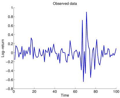
Figure 5: Sampled data $y_{1},\ldots,y_{t_{\max}}$ for the switching stochastic volatility model.

One can then run a sequential Monte Carlo algorithm with the function biips_smc_samples to provide a particle approximation of the posterior distribution. The particle filter can be run in filtering, smoothing and/or backward smoothing modes, see (Doucet and Johansen, 2011) for more details. By default, Biips also automatically chooses the proposal distribution $q_{t}$.

Matbiips

⬇

n_part = 5000;

variables = {’x’};

out_smc = biips_smc_samples(model, variables, n_part);

diag_smc = biips_diagnosis(out_smc);

Rbiips

⬇

n_part <- 5000

variables <- c(’x’)

out_smc <- biips_smc_samples(model, variables, n_part)

diag_smc <- biips_diagnosis(out_smc)

out_smc is an object containing the values of the particles and their weights for each of the monitored variables (the variable $X_{1:t_{\max}}$ in the example). An illustration of the weighted particles is given in Figure 6(a). Figure 6(b) shows the value of the SESS with respect to time. If the minimum is below the threshold of 30, biips_diagnosis recommends to increase the number of particles.

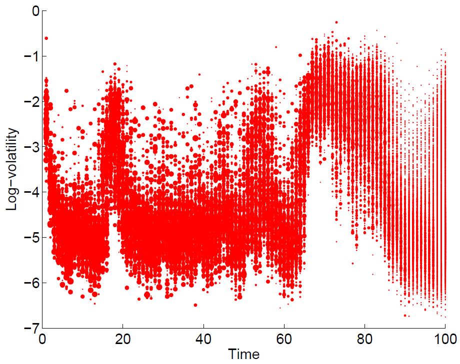
(a) Particles (smoothing)

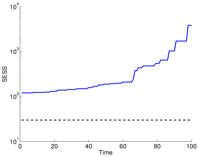
(b) SESS

Figure 6: SMC: (a) Set of weighted particles of the posterior distribution for the switching stochastic volatility model. (b) Smoothing effective sample size with respect to $t$.

The function biips_summary provides some summary statistics on the marginal distributions (mean, quantiles, etc.), and biips_density returns kernel density estimates of the marginal posterior distributions.

Matbiips

⬇

summ_smc = biips_summary(out_smc, ’probs’, [.025, .975]);

x_f_mean = summ_smc.x.f.mean; x_f_quant = summ_smc.x.f.quant;

x_s_mean = summ_smc.x.s.mean; x_s_quant = summ_smc.x.s.quant;

kde_smc = biips_density(out_smc);

Rbiips

⬇

summ_smc <- biips_summary(out_smc, probs=c(.025, .975))

x_f_mean <- summ_smc$x$f$mean; x_f_quant <- summ_smc$x$f$quant

x_s_mean <- summ_smc$x$s$mean; x_s_quant <- summ_smc$x$s$quant

kde_smc <- biips_density(out_smc)

Plots of these summary statistics and kernel density estimates are given in Figures 7 and 8.

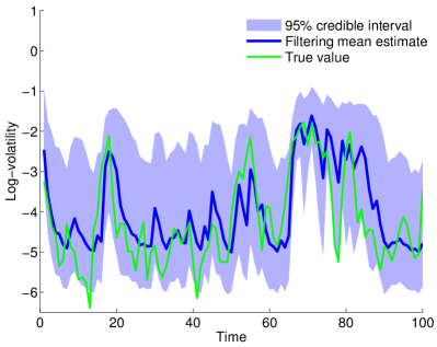
(a) Filtering

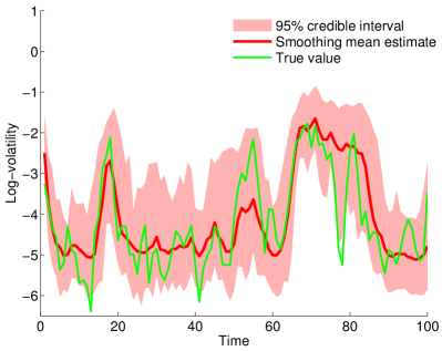
(b) Smoothing

Figure 7: SMC: (a) Filtering and (b) smoothing estimates and credible intervals for the switching stochastic volatility model.

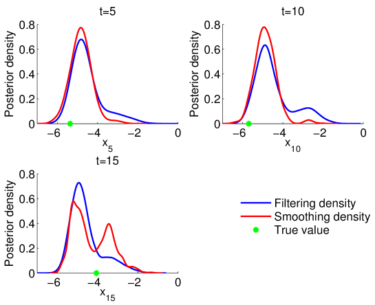
Figure 8: SMC: Kernel density estimates for the marginal posteriors of $X_{t}|Y_{1:t}$ and $X_{t}|Y_{1:t_{\text{max}}}$ for $t=5,10,15$.

5.2 Bayesian inference with particle independent Metropolis-Hastings

The SMC algorithm can also be used as a proposal distribution within an MCMC algorithm to provide MCMC samples from the posterior distribution, as described in Section 3.4. This can be done with Biips with the functions biips_pimh_init, biips_pimh_update and biips_pimh_samples. The first function creates a PIMH object; The second one runs burn-in iterations; The third one runs PIMH iterations and returns samples.

Matbiips

⬇

n_burn = 2000; n_iter = 10000; thin = 1; n_part = 50;

obj_pimh = biips_pimh_init(model, variables);

obj_pimh = biips_pimh_update(obj_pimh, n_burn, n_part); % Burn-in iterations

[obj_pimh, out_pimh, log_marg_like_pimh] = biips_pimh_samples(obj_pimh,...

n_iter, n_part, ’thin’, thin); % Return samples

summ_pimh = biips_summary(out_pimh, ’probs’, [.025, .975]);

x_pimh_mean = summ_pimh.x.mean;

x_pimh_quant = summ_pimh.x.quant;

Rbiips

⬇

n_burn <- 2000; n_iter <- 10000; thin <- 1; n_part <- 50

obj_pimh <- biips_pimh_init(model, variables)

biips_pimh_update(obj_pimh, n_burn, n_part) # Burn-in iterations

out_pimh <- biips_pimh_samples(obj_pimh, n_iter, n_part,

thin=thin) # Return samples

summ_pimh <- biips_summary(out_pimh, probs=c(.025, .975))

x_pimh_mean <- summ_pimh$x$mean

x_pimh_quant <- summ_pimh$x$quant

Posterior means, credible intervals and some marginal posteriors are reported in Figure 9.

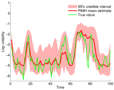
(a) Estimates

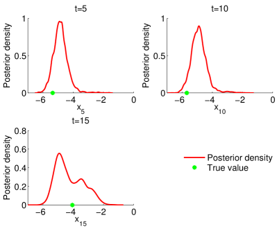
(b) Posterior marginals

Figure 9: PIMH: (a) Smoothing estimates and credible intervals for the switching stochastic volatility model. (b) Posterior marginals $p(x_{t}|y_{1:t_{\max}})$ for $t=5,10,15$.

5.3 Sensitivity analysis with SMC

We now consider evaluating the sensitivity of the model with respect to the model parameters $\alpha_{1}$ and $\alpha_{2}$. For a grid of values of those parameters, we report the estimated logarithm of the marginal likelihood $p(y_{1:t_{\max}})$ using a sequential Monte Carlo algorithm.

Matbiips

⬇

n_part = 50;

param_names = {’alpha’};

[A, B] = meshgrid(-5:.2:2, -5:.2:2);

param_values = {[A(:), B(:)]’};

out_sens = biips_smc_sensitivity(model, param_names, param_values, n_part);

Rbiips

⬇

n_part <- 50

range <- seq(-5,2,.2)

A <- rep(range, times=length(range))

B <- rep(range, each=length(range))

param_values <- list(’alpha’=rbind(A, B))

out_sens <- biips_smc_sensitivity(model, param_values, n_part)

The results are reported in Figure 10.

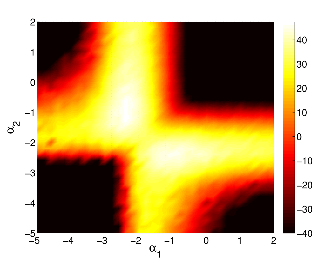
Figure 10: Sensitivity: Estimates of the marginal log-likelihood provided by SMC for different values of $\alpha_{1}$ and $\alpha_{2}$, the other values of the parameters being held fixed. True values are $\alpha_{1}=-2.5$ and $\alpha_{2}=-1$.

5.4 Bayesian inference with unknown parameters with the particle marginal Metropolis-Hastings

So far, we have assumed that the parameters $\alpha$, $\pi$, $\phi$ and $\tau$ were fixed and known. We now consider that these variables have to be estimated as well. We consider the following prior on the parameters (Carvalho and Lopes, 2007):

$$\begin{aligned} \alpha_{1}&=\gamma_{1}\\ \alpha_{2}&=\gamma_{1}+\gamma_{2}\\ \gamma_{1}&\sim\operatorname{\mathcal{N}}(0,100)\\ \gamma_{2}&\sim\operatorname{\mathcal{TN}}_{(0,+\infty)}(0,100)\end{aligned}\qquad\qquad\begin{aligned} \frac{1}{\sigma^{2}}&\sim\operatorname{Gamma}(2.001,1)\\ \phi&\sim\operatorname{\mathcal{TN}}_{(-1,1)}(0,100)\\ \pi_{11}&\sim\operatorname{Beta}(10,1)\\ \pi_{22}&\sim\operatorname{Beta}(10,1)\end{aligned}$$ (7)

where $\operatorname{Gamma}(a,b)$ is the standard Gamma distribution of scale $a>0$ and rate $b>0$, $\operatorname{\mathcal{TN}}_{(a,b)}(\mu,\sigma^{2})$ is the truncated normal distribution of mean $\mu\in\mathbb{R}$ and variance $\sigma^{2}>0$ with support $[a,b]$, $-\infty<a<b<\infty$ and $\operatorname{Beta}(a,b)$ is the standard beta distribution with parameters $a>0$ and $b>0$. Note that the prior on $\phi$ is essentially uniform. Figure 11 shows the representation of the full statistical model as a directed acyclic graph.

Figure 11: Graphical representation of the full switching volatility model defined by Equations (1) and (7) as a directed acyclic graph. Blue and green nodes correspond to unobserved variables, orange nodes to observed variables. In the particle marginal Metropolis-Hastings algorithm, green nodes correspond to variables sampled using a Metropolis-Hastings proposal, whereas blue nodes correspond to variables sampled using a SMC algorithm.

The Listing 2 provides the transcription of the statistical model defined by Equations (1) and (7) in BUGS language.

Listing 2: Switching stochastic volatility model with unknown parameters in BUGS language

⬇

model

{

gamma[1] ~ dnorm(0, 1/100)

gamma[2] ~ dnorm(0, 1/100) T(0,)

alpha[1] <- gamma[1]

alpha[2] <- gamma[1] + gamma[2]

phi ~ dnorm(0, 1/100) T(-1,1)

tau ~ dgamma(2.001, 1)

sigma <- 1/sqrt(tau)

pi[1,1] ~ dbeta(10, 1)

pi[1,2] <- 1 - pi[1,1]

pi[2,2] ~ dbeta(10, 1)

pi[2,1] <- 1 - pi[2,2]

c[1] ~ dcat(pi[1,])

mu[1] <- alpha[1] * (c[1] == 1) + alpha[2] * (c[1] == 2)

x[1] ~ dnorm(mu[1], 1/sigma^2) T(-500,500)

prec_y[1] <- exp(-x[1])

y[1] ~ dnorm(0, prec_y[1])

for (t in 2:t_max)

{

c[t] ~ dcat(ifelse(c[t-1] == 1, pi[1,], pi[2,]))

mu[t] <- alpha[1] * (c[t] == 1) + alpha[2] * (c[t] == 2) + phi * x[t-1]

x[t] ~ dnorm(mu[t], 1/sigma^2) T(-500,500)

prec_y[t] <- exp(-x[t])

y[t] ~ dnorm(0, prec_y[t])

}

}

The user can then load the model and run a PMMH sampler to approximate the joint distribution of $\theta=(\alpha_{1},\alpha_{2},\sigma,\pi_{11},\pi_{22},\phi)$ and $(X_{1},C_{1},\ldots,X_{t_{\max}},C_{t_{\max}})$ given the data $(Y_{1},\ldots,Y_{t_{\max}})$. The function biips_pmmh_init creates a PMMH object. The input param_names contains the names of the variables to be updated using a Metropolis-Hastings proposal, here $(\gamma_{1},\gamma_{2},\tau=\frac{1}{\sigma^{2}},\phi,\pi_{11},\pi_{22})$. Other variables are updated using a SMC algorithm. The input latent_names specifies the other variables for which we want to obtain posterior samples. The function biips_pmmh_update runs a PMMH with adaptation and burn-in iterations. During the adaptation phase, it learns the parameters of the proposal distribution $\nu$ in Algorithm 3.

Matbiips

⬇

sigma_true = .4; alpha_true = [-2.5; -1]; phi_true = .5;

pi11 = .9; pi22 = .9; pi_true = [pi11, 1 - pi11; 1 - pi22, pi22];

data = struct(’t_max’, t_max, ’sigma_true’, sigma_true,...

’alpha_true’, alpha_true, ’phi_true’, phi_true, ’pi_true’, pi_true);

model_file = ’switch_stoch_volatility_param.bug’;

model = biips_model(model_file, data, ’sample_data’, sample_data);

data = model.data;

n_burn = 2000; n_iter = 40000; thin = 10; n_part = 50;

param_names = {’gamma[1]’, ’gamma[2]’, ’phi’, ’tau’, ’pi[1,1]’, ’pi[2,2]’};

latent_names = {’x’, ’alpha[1]’, ’alpha[2]’, ’sigma’};

inits = {-1, 1, .5,5, .8, .8};

obj_pmmh = biips_pmmh_init(model, param_names,...

’inits’, inits, ’latent_names’, latent_names);

obj_pmmh = biips_pmmh_update(obj_pmmh, n_burn, n_part);

[obj_pmmh, out_pmmh, log_marg_like_pen, log_marg_like] =...

biips_pmmh_samples(obj_pmmh, n_iter, n_part, ’thin’, thin);

Rbiips

⬇

sigma_true <- .4; alpha_true <- c(-2.5, -1); phi_true <- .5

pi11 <- .9; pi22 <- .9

pi_true <- matrix(c(pi11, 1-pi11, 1-pi22, pi22), nrow=2, byrow=TRUE)

data <- list(t_max=t_max, sigma_true=sigma_true,

alpha_true=alpha_true, phi_true=phi_true, pi_true=pi_true)

model_file <- ’switch_stoch_volatility_param.bug’

model <- biips_model(model_file, data, sample_data=sample_data)

data <- model$data()

n_burn <- 2000; n_iter <- 40000; thin <- 10; n_part <- 50

param_names <- c(’gamma[1]’, ’gamma[2]’, ’phi’, ’tau’, ’pi[1,1]’, ’pi[2,2]’)

latent_names <- c(’x’, ’alpha[1]’, ’alpha[2]’, ’sigma’)

inits <- list(-1, 1, .5, 5, .8, .8)

obj_pmmh <- biips_pmmh_init(model, param_names, inits=inits,

latent_names=latent_names)

biips_pmmh_update(obj_pmmh, n_burn, n_part)

out_pmmh <- biips_pmmh_samples(obj_pmmh, n_iter, n_part, thin=thin)

Posterior sample traces and histograms of the parameters are given in Figure 12. Posterior means and marginal posteriors for the variables $(X_{1},\ldots,X_{t_{max}})$ and $(C_{1},\ldots,C_{max})$ are given in Figures 13 and 14. The PMMH also returns an estimate of the logarithm of the marginal likelihood at each iteration. The algorithm can therefore also be used as a stochastic search algorithm for finding the marginal MAP of the parameters. The log-marginal likelihood is shown on Figure 15.

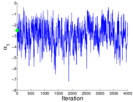
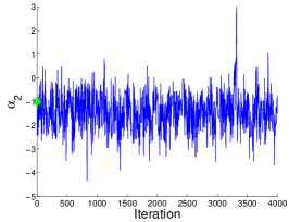
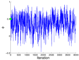
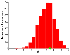
(a) $\alpha_{1}$

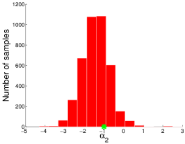
(b) $\alpha_{2}$

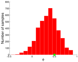
(c) $\phi$

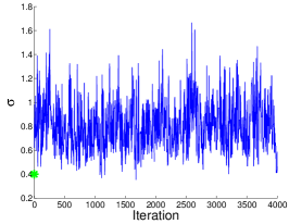
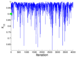
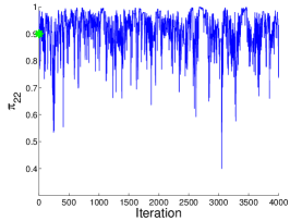
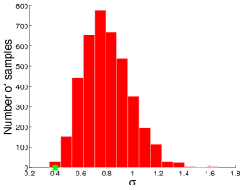
(d) $\sigma$

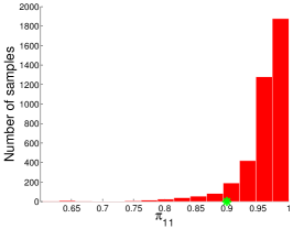
(e) $\pi_{11}$

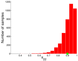
(f) $\pi_{22}$

Figure 12: PMMH: Posterior samples traces (top figures) and histograms (bottom figures) of the parameters (a) $\alpha_{1}$, (b) $\alpha_{2}$, (c) $\phi$, (d) $\sigma$ (e) $\pi_{11}$ and (f) $\pi_{22}$. True values are represented by a green star.

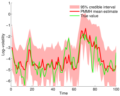
(a) Estimates

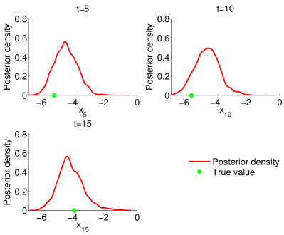
(b) Posterior marginals

Figure 13: PMMH: (a) Smoothing estimates and credible intervals for the switching stochastic volatility model. (b) Posterior marginals $p(x_{t}|y_{1:t_{\max}})$ for $t=5,10,15$.

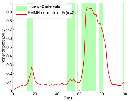
Figure 14: PMMH: Marginal posterior probability $\Pr(C_{t}=2|y_{1},\ldots,y_{t_{max}})$ of being in state 2 over time. Shaded green area corresponds to the true state being in state 2.

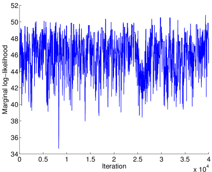
Figure 15: PMMH: Logarithm of the marginal likelihood $p(y_{1},\ldots,y_{t_{max}}|\theta)$ over MCMC iterations.

6 Example: Stochastic kinetic Lotka-Volterra model

We consider now Bayesian inference in the Lotka-Volterra model (Boys et al., 2008). This continuous-time Markov jump process describes the evolution of two species $X_{1}(t)$ (prey) and $X_{2}(t)$ at time $t$, evolving according to the three reaction equations:

$$X_{1}$$ prey reproduction,

predator reproduction,

predator death

(8)

where $c_{1}=0.5$, $c_{2}=0.0025$ and $c_{3}=0.3$ are the rate at which some reaction occur. Let $dt$ be an infinitesimal interval. More precisely, the process evolves as

$$\Pr(X_{1}(t+dt)=x_{1}(t)+1,X_{2}(t+dt)=x_{2}(t)|x_{1}(t),x_{2}(t)) =c_{1}x_{1}(t)dt+o(dt)$$ (9a)

$$\Pr(X_{1}(t+dt)=x_{1}(t)-1,X_{2}(t+dt)=x_{2}(t)+1|x_{1}(t),x_{2}(t)) =c_{2}x_{1}(t)x_{2}(t)dt+o(dt)$$ (9b)

$$\Pr(X_{1}(t+dt)=x_{1}(t),X_{2}(t+dt)=x_{2}(t)-1|x_{1}(t),x_{2}(t)) =c_{3}x_{2}(t)dt+o(dt).$$ (9c)

Forward simulation from the model (9) can be done using the Gillespie algorithm (Gillespie, 1977; Golightly and Gillespie, 2013). We additionally assume that we observe at some time $t=1,2,\ldots,t_{\max}$ the number of preys with some additive noise

$$Y(t)=X_{1}(t)+\epsilon(t),~{}~{}\epsilon(t)\sim\operatorname{\mathcal{N}}(0,\sigma^{2})$$ (10)

The objective is to approximate the posterior distribution on the number of preys and predators $(X_{1}(t),X_{2}(t))$ at $t=1,\ldots,t_{\max}$ given the data $(Y(1),\ldots,Y(t_{\max}))$. Listing 3 gives the transcription of the model defined by Equations (9) and (10) in the BUGS language.

Listing 3: Stochastic kinetic model in BUGS language

⬇

model

{

x[,1] ~ LV(x_init, c[1], c[2], c[3], 1)

y[1] ~ dnorm(x[1,1], 1/sigma^2)

for (t in 2:t_max)

{

x[,t] ~ LV(x[,t-1], c[1], c[2], c[3], 1)

y[t] ~ dnorm(x[1,t], 1/sigma^2)

}

}

The Gillespie sampler to sample from (9) is not part of the BUGS library of samplers. Nonetheless, Biips allows the user to add two sorts of external functions:

1. Deterministic functions, with biips_add_function. Such an external function is called after the symbol <- in BUGS, e.g. y <- f_ext_det(x)

2. Sampling distributions, with the function biips_add_distribution. Such an external sampler is called after the symbol   in BUGS, e.g. z   f_ext_samp(x)

The function ‘LV’ used in the Listing 3 is an additional sampler calling a MATLAB/R custom function to sample from the Lotka-Volterra model using the Gillepsie algorithm.

Matbiips

⬇

function x = lotka_volterra_gillespie(x, c1, c2, c3, dt)

% Matlab function to sample from a Lotka-Volterra model

% with the Gillepsie algorithm

z = [1, -1, 0; 0, 1, -1];

t = 0;

while true

rate = [c1 * x(1), c2 * x(1) * x(2), c3 * x(2)];

sum_rate = sum(rate);

% Sample the next event from an exponential distribution

t = t - log(rand) / sum_rate;

% Sample the type of event

ind = find((sum_rate * rand) <= cumsum(rate), 1);

if t > dt

break

end

x = x + z(:,ind);

end

Rbiips

⬇

lotka_volterra_gillespie <- function(x, c1, c2, c3, dt) {

# R function to sample from a Lotka-Volterra model

# with the Gillepsie algorithm

z <- matrix(c(1, -1, 0, 0, 1, -1), nrow=2, byrow=TRUE)

t <- 0

while (TRUE) {

rate <- c(c1*x[1], c2*x[1]*x[2], c3*x[2])

sum_rate <- sum(rate);

# Sample the next event from an exponential distribution

t <- t - log(runif(1))/sum_rate

# Sample the type of event

ind <- which((sum_rate*runif(1)) <= cumsum(rate))[1]

if (t>dt)

break

x <- x + z[,ind]

}

return(x)

}

One can add the custom function ‘LV’ to Biips, and run a SMC algorithm on the stochastic kinetic model in order to estimate the number of preys and predators. Estimates, together with the true numbers of prey and predators, are reported in Figure 16.

Matbiips

⬇

fun_bugs = ’LV’; fun_nb_inputs = 5;

fun_dim = ’lotka_volterra_dim’; fun_sample = ’lotka_volterra_gillespie’;

biips_add_distribution(fun_bugs, fun_nb_inputs, fun_dim, fun_sample);

t_max = 40; x_init = [100; 100]; c = [.5, .0025, .3]; sigma = 10;

data = struct(’t_max’, t_max, ’c’, c, ’x_init’, x_init, ’sigma’, sigma);

model_file = ’stoch_kinetic_gill.bug’; sample_data = true;

model = biips_model(model_file, data, ’sample_data’, sample_data);

n_part = 10000; variables = {’x’};

out_smc = biips_smc_samples(model, variables, n_part);

summ_smc = biips_summary(out_smc, ’probs’, [.025, .975]);

Rbiips

⬇

fun_bugs <- ’LV’; fun_nb_inputs <- 5

fun_dim <- lotka_volterra_dim; fun_sample <- lotka_volterra_gillespie

biips_add_distribution(fun_bugs, fun_nb_inputs, fun_dim, fun_sample)

t_max <- 40; x_init <- c(100, 100); c <- c(.5, .0025, .3); sigma <- 10

data <- list(t_max=t_max, c=c, x_init=x_init, sigma=sigma)

model_file <- ’stoch_kinetic_gill.bug’; sample_data=TRUE

model <- biips_model(model_file, data, sample_data=sample_data)

n_part <- 10000 ; variables <- c(’x’)

out_smc <- biips_smc_samples(model, variables, n_part)

summ_smc <- biips_summary(out_smc, probs=c(.025, .975))

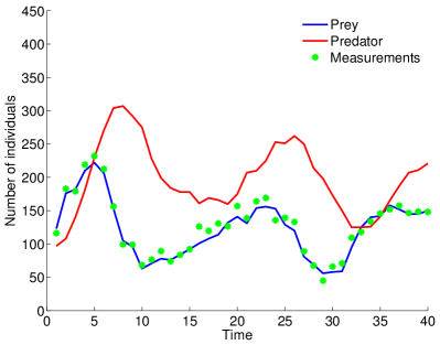
(a) Ground truth and data

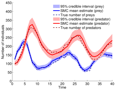
(b) Estimates

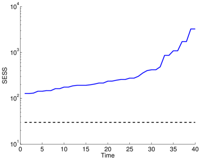
(c) Smoothing effective sample size

Figure 16: Stochastic kinetic model: (a) True number of prey/predators and measurements. (b) Estimated number of prey/predators and 95% credible intervals. (c) Smoothing effective sample size.

7 Discussion of related software

7.1 Related software for Bayesian inference using MCMC

Biips belongs to the BUGS language software family of WinBUGS, OpenBUGS (Lunn et al., 2000, 2012) and JAGS software (Plummer, 2003). All these probabilistic programming software use BUGS as a language for describing the statistical model.

In particular, Biips is written in C++ like JAGS but unlike Win/OpenBUGS which is written in Component Pascal. This was a good reason for adapting JAGS implementation of the BUGS language which might slightly differ from the Win/OpenBUGS original one.

Like the above software, Biips compiles the model at runtime, by dynamically allocating instances of node classes. The resulting graphical model might have a substantial memory size. Stan (Stan Development Team, 2013) is a similar software which uses another strategy. It translates the model description into C++ code that is transformed into an executable at compile-time. This might result in lower memory occupancy and faster execution, at the cost of a longer compilation. In addition, Stan implements its own language for model definition. In particular, Stan language is imperative as opposed to the declarative nature of BUGS.

The main difference between Biips and the aforementioned software is that Biips uses SMC instead of MCMC as inference algorithm.

7.2 Related software for Bayesian inference using SMC

SMCTC (Johansen, 2009) is a C++ template class library offering a generic framework for implementing SMC methods. It does not come with many features though and might require a lot of coding and understanding of SMC from the user. The development of Biips has started by adapting this library and providing it with more user-friendly features. This template is extended in vSMC (Zhou, 2013) to directly support parallelisation. RCppSMC (Eddelbuettel and Johansen, 2014) provides an R interface to SMCTC.

LibBi (Murray, 2013) is another similar software that implements SMC methods and is suited to parallel and distributed computer hardware such as multi-core CPUs, GPUs and clusters. LibBi comes with its own modeling language although restricting to the state-space model framework. Like Stan, LibBi transforms the model definition into an executable at compile-time, resulting in high computing performances.

Other software such as Venture (Mansinghka et al., 2014) or Anglican (Wood et al., 2014) also propose particle MCMC inference engines for posterior inference, with a different probabilistic language, that allows for more expressiveness; in particular, it can deal with models of changing dimensions, complex control flow or stochastic recursion.

7.3 Related software for stochastic optimization

Although the focus of Biips is automatic Bayesian inference, interacting particle methods have long been successfully used for stochastic optimization. These algorithms use similar exploration/selection steps and are usually known under the names of evolutionary algorithms, genetic algorithms or meta-heuristics. Several softwares have been developed over the past few years, such as EASEA (Collet et al., 2000), Evolver or ParadisEO (Cahon et al., 2004).

8 Conclusion

The Biips software is a BUGS compatible, black-box inference engine using sequential Monte Carlo methods. Due to its use of the BUGS language, and the ability to define custom functions/distributions, it allows a lot of flexibility in the development of statistical models. By using particle methods, the software can return estimates of the marginal likelihood at no additional cost, and can use custom conditional distributions, possibly with an intractable expression. Although particle methods are particularly suited to posterior inference on the two examples discussed in this paper, Biips running times are still higher than those of a more mature software with a MCMC inference engine such as JAGS. Nonetheless, there is room for improvement and optimization of Biips; in particular, particle algorithms are particularly suited to parallelization (Lee et al., 2010; Vergé et al., 2013; Murray, 2013), and we plan in future releases of the software to provide a parallel implementation of Biips.

Acknowledgement.

The authors thank Arnaud Doucet, Pierre Jacob, Adam Johansen and Frank Wood for useful feedback on earlier versions of the paper. François Caron acknowledges the support of the European Commission under the Marie Curie Intra-European Fellowship Programme.

References

- Andrieu et al. (2010) Andrieu C, Doucet A, Holenstein R (2010). “Particle Markov Chain Monte Carlo Methods.” Journal of the Royal Statistical Society B, 72, 269–342.
- Bouchard-Côté et al. (2012) Bouchard-Côté A, Sankararaman S, Jordan MI (2012). “Phylogenetic inference via sequential Monte Carlo.” Systematic biology, 61(4), 579–593.
- Boys et al. (2008) Boys RJ, Wilkinson DJ, Kirkwood TBL (2008). “Bayesian Inference for a Discretely Observed Stochastic Kinetic Model.” Statistics and Computing, 18(2), 125–135.
- Buckland et al. (2007) Buckland ST, Newman KB, Fernandez C, Thomas L, Harwood J (2007). “Embedding population dynamics models in inference.” Statistical Science, pp. 44–58.
- Cahon et al. (2004) Cahon S, Melab N, Talbi EG (2004). “\pkgParadisEO: A Framework for the Reusable Design of Parallel and Distributed Metaheuristics.” Journal of Heuristics, 10(3), 357–380.
- Cappé et al. (2005) Cappé O, Moulines E, Ryden T (2005). Inference in Hidden Markov Models. Springer.
- Cappé and Robert (2000) Cappé O, Robert C (2000). “Markov Chain Monte Carlo: 10 years and Still Running!” Journal of the American Statistical Association, 95, 1282–1286.
- Caron et al. (2008) Caron F, Davy M, Doucet A, Duflos E, Vanheeghe P (2008). “Bayesian Inference for Linear Dynamic Models with Dirichlet Process Mixtures.” IEEE Transactions on Signal Processing, 56(1), 71–84.
- Caron et al. (2007) Caron F, Davy M, Duflos E, Vanheeghe P (2007). “Particle filtering for multisensor data fusion with switching observation models: Application to land vehicle positioning.” IEEE Transactions on Signal Processing, 55(6), 2703–2719.
- Caron et al. (2012) Caron F, Doucet A, Gottardo R (2012). “On-line Changepoint Detection and Parameter Estimation with Application to Genomic Data.” Statistics and Computing, 22(2), 579–595.
- Carvalho and Lopes (2007) Carvalho CM, Lopes HF (2007). “Simulation-based Sequential Analysis of Markov Switching Stochastic Volatility Models.” Computational Statistics & Data Analysis, 51(9), 4526–4542.
- Cauchemez et al. (2008) Cauchemez S, Valleron AJ, Boelle P, Flahault, Ferguson NM (2008). “Estimating the impact of school closure on influenza transmission from Sentinel data.” Nature, 452(7188), 750–754.
- Collet et al. (2000) Collet P, Lutton E, Schoenauer M, Louchet J (2000). “Take it \pkgEASEA.” In Parallel Problem Solving from Nature PPSN VI, pp. 891–901. Springer.
- Del Moral (2004) Del Moral P (2004). Feynman-Kac Formulae. Genealogical and Interacting Particle Systems with Application. Springer.
- Del Moral (2013) Del Moral P (2013). Mean Field Simulation for Monte Carlo Integration. Chapman and Hall/CRC.
- Del Moral et al. (2012) Del Moral P, Peters GW, Vergé C (2012). “An introduction to particle integration methods: with applications to risk and insurance.” In Monte Carlo and Quasi-Monte Carlo Methods. Springer-Verlag.
- Donnet and Samson (2011) Donnet S, Samson A (2011). “EM algorithm coupled with particle filter for maximum likelihood parameter estimation of stochastic differential mixed-effects models.” Technical report.
- Douc et al. (2014) Douc R, Moulines E, Stoffer DS (2014). Nonlinear Time Series. CRC Press.
- Doucet et al. (2001) Doucet A, de Freitas N, Gordon N (eds.) (2001). Sequential Monte Carlo Methods in Practice. Springer-Verlag.
- Doucet et al. (2000) Doucet A, Godsill S, Andrieu C (2000). “On Sequential Monte Carlo Sampling Methods for Bayesian Filtering.” Statistics and Computing, 10(3), 197–208.
- Doucet and Johansen (2011) Doucet A, Johansen A (2011). “A Tutorial on Particle Filtering and Smoothing: Fifteen Years Later.” In D Crisan, B Rozovsky (eds.), Oxford Handbook of Nonlinear Filtering. Oxford University Press.
- Dureau et al. (2013) Dureau J, Kalogeropoulos K, Baguelin M (2013). “Capturing the time-varying drivers of an epidemic using stochastic dynamical systems.” Biostatistics, p. kxs052.
- Eddelbuettel (2013) Eddelbuettel D (2013). Seamless \proglangR and \proglangC++ Integration with \pkgRcpp. Springer, New York. ISBN 978-1-4614-6867-7.
- Eddelbuettel and François (2011) Eddelbuettel D, François R (2011). “\pkgRcpp: Seamless \proglangR and \proglangC++ Integration.” Journal of Statistical Software, 40(8), 1–18. URL http://www.jstatsoft.org/v40/i08/.
- Eddelbuettel and Johansen (2014) Eddelbuettel D, Johansen AM (2014). \pkgRcppSMC: \pkgRcpp bindings for Sequential Monte Carlo. \proglangR package version 0.1.4.
- Fearnhead (2004) Fearnhead P (2004). “Particle Filters for Mixture Models with an Unknown Number of Components.” Statistics and Computing, 14(1), 11–21.
- Fearnhead and Liu (2007) Fearnhead P, Liu Z (2007). “On-line Inference for Multiple Changepoint Problems.” Journal of the Royal Statistical Society B, 69(4), 589–605.
- Fernández-Villaverde and Rubio-Ramírez (2007) Fernández-Villaverde J, Rubio-Ramírez JF (2007). “Estimating macroeconomic models: A likelihood approach.” The Review of Economic Studies, 74(4), 1059–1087.
- Flury and Shephard (2011) Flury T, Shephard N (2011). “Bayesian inference based only on simulated likelihood: particle filter analysis of dynamic economic models.” Econometric Theory, 27(05), 933–956.
- Gilks et al. (1995) Gilks W, Richardson S, Spiegelhalter D (eds.) (1995). Markov Chain Monte Carlo in Practice. Chapman & Hall/CRC.
- Gilks et al. (1994) Gilks W, Thomas A, Spiegelhalter D (1994). “A Language and Program for Complex Bayesian Modelling.” The Statistician, 43, 169–177.
- Gillespie (1977) Gillespie DT (1977). “Exact Stochastic Simulation of Coupled Chemical Reactions.” The journal of physical chemistry, 81(25), 2340–2361.
- Golightly and Gillespie (2013) Golightly A, Gillespie CS (2013). “Simulation of Stochastic Kinetic Models.” In In Silico Systems Biology, pp. 169–187. Springer.
- Golightly and Wilkinson (2006) Golightly A, Wilkinson D (2006). “Bayesian sequential inference for stochastic kinetic biochemical network models.” Journal of Computational Biology, 13(3), 838–851.
- Golightly and Wilkinson (2011) Golightly A, Wilkinson D (2011). “Bayesian parameter inference for stochastic biochemical network models using particle Markov chain Monte Carlo.” Interface Focus, p. rsfs20110047.
- Green et al. (2003) Green PJ, Hjort NL, Richardson S (eds.) (2003). Highly Structured Stochastic Systems. Oxford University Press.
- Gustafsson et al. (2002) Gustafsson F, Gunnarsson F, Bergman N, Forssell U, Jansson J, Karlsson R, Nordlund PJ (2002). “Particle filters for positioning, navigation, and tracking.” IEEE Transactions on Signal Processing, 50(2), 425–437.
- Johansen (2009) Johansen A (2009). “\pkgSMCTC: Sequential Monte Carlo in \proglangC++.” Journal of Statistical Software, 30, 1–41.
- Jordan (2004) Jordan MI (2004). “Graphical Models.” Statistical Science, 19, 140–155.
- Lauritzen (1996) Lauritzen S (1996). Graphical Models. Oxford Science Publications.
- Lee et al. (2010) Lee A, Yau C, Giles MB, Doucet A, Holmes CC (2010). “On the Utility of Graphics Cards to Perform Massively Parallel Simulation of Advanced Monte Carlo Methods.” Journal of Computational and Graphical Statistics, 19(4), 769–789.
- Liu (2001) Liu J (2001). Monte Carlo Strategies in Scientific Computing. Springer.
- Lunn et al. (2012) Lunn D, Jackson C, Best N, Thomas A, Spiegelhalter D (2012). The \pkgBUGS Book: A Practical Introduction to Bayesian Analysis. CRC Press/ Chapman and Hall.
- Lunn et al. (2000) Lunn D, Thomas A, Best N, Spiegelhalter D (2000). “\pkgWinBUGS - a Bayesian Modelling Framework: Concepts, Structure and Extensibility.” Statistics and Computing, 10, 325–337.
- Mansinghka et al. (2014) Mansinghka VK, Selsam D, Perov YN (2014). “\pkgVenture: A Higher-order Probabilistic Programming Platform with Programmable Inference.” Technical report, arXiv:1404.0099.
- Murray (2013) Murray L (2013). “Bayesian State-Space Modelling on High-Performance Hardware Using \pkgLibBi.” Technical report, CSIRO. Arxiv:1306.3277.
- Naesseth et al. (2014) Naesseth CA, Lindsten F, Schön TB (2014). “Sequential Monte Carlo for Graphical Models.” In Advances in Neural Information Processing Systems (NIPS).
- Peters et al. (2010) Peters GW, Hosack GR, Hayes KR (2010). “Ecological non-linear state space model selection via adaptive particle Markov chain Monte Carlo (AdPMCMC).” arXiv preprint arXiv:1005.2238.
- Pitt and Shephard (1999) Pitt M, Shephard N (1999). “Filtering via simulation: Auxiliary particle filters.” Journal of the American statistical association, 94(446), 590–599.
- Plummer (2003) Plummer M (2003). “\pkgJAGS: A Program for Analysis of Bayesian Graphical Models using Gibbs Sampling.” In Proceedings of the 3rd International Workshop on Distributed Statistical Computing.
- Plummer (2012) Plummer M (2012). \pkgJAGS Version 3.3.0 user manual.
- Plummer (2014) Plummer M (2014). \pkgrjags: Bayesian graphical models using MCMC. \proglangR package version 3-13, URL http://CRAN.R-project.org/package=rjags.
- Ristic et al. (2004) Ristic B, Arulampalam S, Gordon N (2004). Beyond the Kalman filter: Particle filters for tracking applications, volume 685. Artech house Boston.
- Robert and Casella (2004) Robert C, Casella G (2004). Monte Carlo Statistical Methods. Springer.
- Stan Development Team (2013) Stan Development Team (2013). “\pkgStan: A \proglangC++ Library for Probability and Sampling, Version 2.1.” URL http://mc-stan.org/.
- Thrun et al. (2001) Thrun S, Fox D, Burgard W, Dellaert F (2001). “Robust Monte Carlo localization for mobile robots.” Artificial intelligence, 128(1), 99–141.
- Vergé et al. (2013) Vergé C, Dubarry C, Del Moral P, Moulines E (2013). “On Parallel Implementation of Sequential Monte Carlo Methods: The Island Particle Model.” Statistics and Computing, to appear.
- Vermaak et al. (2002) Vermaak J, Andrieu C, Doucet A, Godsill SJ (2002). “Particle methods for Bayesian modeling and enhancement of speech signals.” IEEE Transactions on Speech and Audio Processing, 10(3), 173–185.
- Vo et al. (2003) Vo BN, Singh S, Doucet A (2003). “Sequential Monte Carlo implementation of the PHD filter for multi-target tracking.” In Proc. International Conference on Information Fusion, pp. 792–799.
- Wood et al. (2014) Wood F, van de Meent JW, Mansinghka V (2014). “A New Approach to Probabilistic Programming Inference.” In Proceedings of the 17th International conference on Artificial Intelligence and Statistics.
- Zhou (2013) Zhou Y (2013). “\pkgvSMC: Parallel Sequential Monte Carlo in \proglangC++.” Technical report, University of Warwick. ArXiv:1306.5583.