Analysis and control of pre-extinction dynamics in stochastic populations

Abstract

We consider a stochastic population model where the intrinsic or demographic noise causes cycling between states before the population eventually goes extinct. A master equation approach coupled with a WKB (Wentzel-Kramers-Brillouin) approximation is used to construct the optimal path to extinction. In addition, a probabilistic argument is used to understand the pre-extinction dynamics and approximate the mean time to extinction. Analytical results agree well with numerical Monte Carlo simulations. A control method is implemented to decrease the mean time to extinction. Analytical results quantify the effectiveness of the control and agree well with numerical simulations.

1 Introduction

It has long been known that noise can significantly affect physical and biological dynamical systems at a wide variety of levels. For example, in biology, noise can play a role in sub-cellular processes, tissue dynamics, and large-scale population dynamics (Tsimring, 2014). Stochasticity can arise in a number of ways. For example, in epidemiological models, noise is due to the random interactions of individuals in a population as well as uncertainty in epidemic parameter values (Rand and Wilson, 1991; Billings et al., 2002). In population ecology, noise may be the result of environmental factors including climatic effects, natural enemies, or inter-specific competition, or may be due to demography (Coulson et al., 2004).

Stochasticity manifests itself as either external or internal noise. External noise comes from a source outside the system being considered (e.g the growth of a species under climatic effects), and often is modeled by replacing an external parameter with a random process. Internal noise is inherent in the system itself and is caused by the random interactions of discrete particles (e.g. individuals in a population). In this article, we are interested in the dynamics of an isolated single-species population undergoing a set of random gain-loss processes that simulate births and deaths. Thus, in this particular case, the internal noise of the population model is demographic noise. Mathematically, the effects of these random interactions are described using a master equation (van Kampen, 2007). Small fluctuations captured in this modeling approach may act as an effective force that drives the population to extinction (Assaf and Meerson, 2010). While population extinction is assumed to be a rare event, we can study these models to theoretically understand pre-extinction dynamics and extinction risk.

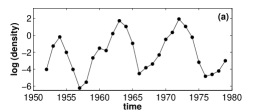
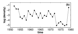
Figure 1: Population density fluctuations of Lepidoptera feeding on larch foliage in the Oberengadin Valley of Switzerland. Data from (Baranchikov et al., 1991) reported as the natural logarithm of numbers per 1000 kg of larch foliage: (a) Exapate duratella (Tortricidae) and (b) Teleia saltuum (Gelechidae).

Extinction risk is an important question in both population dynamics (Thomas et al., 2004) and ecological community dynamics (Ebenman and Jonsson, 2005). For single populations, it has long been recognized that extinction risk is dependent on the carrying capacity of the model (Leigh, 1981; Lande, 1993). Mathematically, the carrying capacity is a positive stable equilibrium in the deterministic model. In this paper, we consider a population with multiple deterministic stable equilibria where the population size can stochastically fluctuate between these states. One such example can be found in the data of forest Lepidoptera (Baranchikov et al., 1991) as shown in Fig. 1. The drastic population shifts are attributed to a mix of parasitoids, viral outbreak among the moths, and the quality of the available foliage (Berryman, 1996). Figure 1(a) shows that the fluctuations may be regular, although they are not seasonal, while Fig. 1(b) shows a switch between two states, with vastly different residence times in each state. Similar fluctuations are observed in the context of human physiology. For example, neural switching and enzyme level cycling are explored in (Elf and Ehrenberg, 2004; Berndt et al., 2009; Samoilov et al., 2005). Regardless of the specific context, it is useful to increase our understanding of pre-extinction dynamics, as well as the mean time to extinction and the path that optimizes the probability of extinction.

In this article, we explore all of these features for a stochastic model that exhibits extinction and for a stochastic model that exhibits pre-extinction cycling that serves to delay the extinction event. The layout for the article is as follows. Section 2 presents the master equation formalism needed to investigate demographic noise in population models and the general method to find the mean time to extinction. A simple population model exhibiting extinction is presented in Section 3. It provides an example of the analytical and numerical methods used to find the mean time to extinction. Pre-extinction cycling is considered in Section 4 and the probabilistic result used to describe pre-extinction dynamics is derived. A control term is introduced in Section 5 to increase the rate of extinction in the model. The methods from the previous sections are used to quantify the effects of the control. In the last section, we generalize these results and give a brief discussion.

2 General Theory

2.1 Master Equation Formalism

As mentioned in the introduction, to study the effects of internal noise on the dynamics of a population, a stochastic model must be considered. If the transitions between states are short and uncorrelated, the system is a Markov process and the evolution of the probability is described by a master equation. In the master equation formulation, the probability of the system taking on a particular state $X$ (number of agents), at a given time $t$, is described by $\rho(X,t)$. Let $W(X;r)$ represent the transition rate from a state $X$ to $X+r$, where $r$ can be a positive or negative integer. In this case the time evolution of $\rho(X,t)$ can be written as (van Kampen, 2007):

$$\frac{d\rho(X,t)}{dt}=\sum_{r}\left[W(X-r;r)\rho\left(X-r,t\right)-W(X;r)\rho(X,t)\right].$$ (1)

We introduce a rescaled coordinate $x=X/K$, where $K$ is the large parameter of the problem. The transition rates are represented as the following expansion in $K$:

$$W(X;r)\equiv W(Kx;r)=Kw_{r}(x)+u_{r}(x)+\mathcal{O}(1/K),$$ (2)

where $x=\mathcal{O}(1)$, and $w_{r}(x)$ and $u_{r}(x)$ also are $\mathcal{O}(1)$.

For $K\gg 1$ the WKB (Wentzel-Kramers-Brillouin) approximation for the scaled master equation can be used (Kubo et al., 1973; Gang, 1987; Dykman et al., 1994; Elgart and Kamenev, 2004; Kessler and Shnerb, 2007; Forgoston et al., 2011; Schwartz et al., 2011). Accordingly, we look for the probability distribution in the form of the WKB ansatz

$$\rho(x,t)=\exp(-K{\cal S}(x,t)),$$ (3)

where ${\cal S}(x,t)$ is a function known as the action.

We substitute Eq. (3) into the scaled master equation which contains terms with the form $w_{r}(x-r/K)$ and ${\cal S}(x-r/K,t)$, where $r/K$ is small. By performing a Taylor series expansion of these functions of $x-r/K$, one arrives at the leading order Hamilton-Jacobi equation $\mathcal{H}(x,p)=0$, where

$$\mathcal{H}(x,p)=\sum_{r}w_{r}(x)\left(\exp(pr)-1\right)$$ (4)

is the effective Hamiltonian, where $p$ is the conjugate momentum and is defined as $p=d{\cal S}/dx$. In this article, we are interested in the special case of a single step process, for which the only values of $r$ are $+1$ and $-1$. The Hamiltonian for a single step process will have the general form

$$\mathcal{H}(x,p)=w_{1}(x)\left(\exp(p)-1\right)+w_{-1}(x)\left(\exp(-p)-1\right).$$ (5)

From the Hamiltonian in Eq. (4), one can easily derive Hamilton’s equations

$$\dot{x}=\frac{\partial\mathcal{H}(x,p)}{\partial p},\qquad\dot{p}=-\frac{\partial\mathcal{H}(x,p)}{\partial x}.$$ (6)

The $x$ dynamics along the $p=0$ deterministic line can be described by the equation

$$\dot{x}=\left.\frac{\partial\mathcal{H}(x,p)}{\partial p}\right|_{p=0}=\sum\limits_{r}rw_{r}(x),$$ (7)

which is simply the rescaled mean-field rate equation associated with the deterministic problem. For a single step process, this simplifies to $\dot{x}=w_{1}(x)-w_{-1}(x)$.

2.2 Mean Time to Extinction

We are interested in how intrinsic noise can cause extinction events of long-lived stochastic populations. In this article, the extinct state $x_{0}$ is an attracting point of the deterministic mean-field equation. Furthermore, there is an intermediate repelling point $x=x_{1}$ between the attracting extinct state and another attracting point $x=x_{2}$. This scenario can be visualized in Fig. 2 and corresponds to a scenario B extinction as explored in (Assaf and Meerson, 2010).

In this extinction scenario, the most probable path to extinction, or optimal path to extinction, is composed of two segments. The first segment is a heteroclinic trajectory with non-zero momentum that connects the equilibrium point $(x,p)=(x_{2},0)$, where $x_{2}$ is an attracting fixed point of the deterministic mean-field equation, with an intermediate equilibrium point $(x,p)=(x_{1},0)$, where $x_{1}$ is a repelling fixed point of the deterministic mean-field equation. The second segment consists of the segment along $p=0$ from $x_{1}$ to the extinct state $x_{0}$.

The optimal path to extinction $p_{opt}(x)$ between $(x_{2},0)$ and $(x_{1},0)$ is a zero energy phase trajectory of the Hamiltonian given by Eq. (4). In a single step process, the optimal path will always have the general form

$$p_{opt}(x)=\ln{\left(w_{-1}(x)/w_{1}(x)\right)}.$$ (8)

Using the definition of the conjugate momentum $p=d{\cal S}/dx$, the action ${\cal S}_{opt}$ along the optimal path $p_{opt}(x)$ is given by

$${\cal S}_{opt}=\int_{x_{2}}^{x_{1}}p_{opt}(x)dx.$$ (9)

Therefore, the mean time to extinction (MTE) to escape from $(x_{2},0)$ and arrive at $(x_{1},0)$ can be approximated by

$$\tau=B\exp({K{\cal S}_{opt}}),$$ (10)

where $B$ is a prefactor that depends on the system parameters and on the population size. An accurate approximation of the MTE depends on obtaining $B$.

To capture the deterministic contribution from $x_{1}$ to $x_{0}$ in the MTE approximation, we include the prefactor derived in (Assaf and Meerson, 2010). Specifically, the following equation is the general form of the MTE for a single-step scenario B extinction from $x_{2}$ to $x_{0}$:

$$\tau_{20}=\frac{2\pi\exp\left(\int_{x_{1}}^{x_{2}}\left(\frac{u_{1}(x)}{w_{1}(x)}-\frac{u_{-1}(x)}{w_{-1}(x)}\right)dx\right)}{w_{1}(x_{2})\sqrt{|p^{\prime}_{opt}(x_{1})|p^{\prime}_{opt}(x_{2})}}\exp\left(K\int_{x_{2}}^{x_{1}}\ln\left(\frac{w_{-1}(x)}{w_{1}(x)}\right)dx\right).$$ (11)

Note that we will use the general notation $\tau_{ij}$ to identify the function $\tau_{ij}(x_{i},x_{(i+j)/2})$ that provides the escape time from state $x_{i}$ to state $x_{j}$. In the case that $i=2$ and $j=0$, then one recovers Eq. (11). It is worth noting that the derivation of Eq. (11) involves matching the solution from $x_{2}$ to $x_{1}$ asymptotically with the deterministic solution from $x_{1}$ to $x_{0}$. Because this latter solution is associated with $p=0$, its final form does not involve an integral from $x_{1}$ to $x_{0}$. Nevertheless, the deterministic contribution is in fact included in Eq. (11).

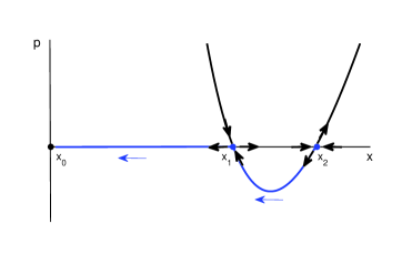
Figure 2: Zero-energy trajectories $p=0$, $x=0$, and $p_{opt}(x)$ of the Hamiltonian for the stochastic Allee population model given by Eq. (13). The optimal path to extinction (blue curve) consists of the heteroclinic trajectory $p_{opt}(x)$ (Eq. (16)) connecting $x_{2}$ to $x_{1}$, and the $p=0$ line from $x_{1}$ to the extinct state $x_{0}$.

3 An example of extinction

To illustrate the analytical methods described in Sec. 2, we consider an example where the local dynamics of a population exhibit the Allee effect. The Allee effect is seen in animal populations that benefit from conspecific cooperation. These populations tend to perform better in larger numbers. In fact, there is evidence that larger populations are more capable of avoiding predation, can reproduce faster, and are better able to resist toxic environmental conditions (Allee, 1931; Lidicker Jr, 2010). On the other hand, the growth rate is negative for low densities. Therefore the dynamics are bistable and the population will tend towards a positive state, referred to as the carrying capacity, or an extinct state depending on the initial population. A simple deterministic mathematical model demonstrating the Allee effect can be written as $\dot{x}=f(x)$, where $f(x)$ is a cubic polynomial. Using the notation used in Fig. 2, we could write $f(x)=x(x-x_{1})(x-x_{2})$. The corresponding stochastic population model is represented by the following transition processes and associated rates $W(X;r)$.

Transition	W(X;r)
${\displaystyle X\overset{\mu}{\longrightarrow}\varnothing}$	$\mu X$,
${\displaystyle 2X\overset{\lambda/K}{\longrightarrow}3X}$	$\lambda\frac{X(X-1)}{2K}$,
${\displaystyle 3X\overset{\sigma/K^{2}}{\longrightarrow}2X}$	$\sigma\frac{X(X-1)(X-2)}{6K^{2}}$.

The first two transitions are required to capture the Allee effect. The death rate of a low-density population is given by $\mu$, and the growth rate of the population when the density is large enough is given by $\lambda$. The negative growth rate for an overcrowded population is provided by $\sigma$, and $K$ is the carrying capacity of the population.

As described in Sec. 2, the transition processes and their associated rates are used to formulate the master equation given by Eq. (1). In this particular example, all of the transitions are single-step transitions. Therefore, the increment $r$ only takes on the values of $\pm 1$. The scaled transition rates in Eq. (2) are given as

$$\begin{array}[]{lll}w_{1}(x)=\frac{\lambda x^{2}}{2},&{}{}{}{}{}&w_{-1}(x)=\mu x+\frac{\sigma x^{3}}{6},\\ &&\\ u_{1}(x)=-\frac{\lambda x}{2},&{}{}{}{}{}&u_{-1}(x)=-\frac{\sigma x^{2}}{2}.\end{array}$$ (12)

Substitution of Eq. (12) into Eq. (4) leads to the following Hamiltonian:

$$\mathcal{H}(x,p)=\frac{\lambda x^{2}}{2}(e^{p}-1)+\left(\mu x+\frac{\sigma x^{3}}{6}\right)(e^{-p}-1).$$ (13)

Taking derivatives of Eq. (13) with respect to $p$ and $x$ (Eq. (6)) lead to the following system of Hamilton’s equations:

$$\dot{x} = \frac{\lambda x^{2}}{2}e^{p}-\left(\mu x+\frac{\sigma x^{3}}{6}\right)e^{-p}$$ (14)

$$\dot{p} = -\lambda x(e^{p}-1)-\left(\mu+\frac{\sigma x^{2}}{2}\right)(e^{-p}-1).$$ (15)

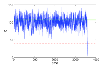
Figure 3: A single realization exhibiting extinction in the stochastic Allee population model. The non-zero deterministic stable state is shown by the green line, while the deterministic unstable state is shown by the red dashed line. The parameter values are $\mu=0.2$, $\sigma=3.0$, $\lambda=1.425$, and $K=100$.

By setting the Hamiltonian in Eq. (13) equal to zero and solving for $p$ and $x$ it is possible to find three zero-energy phase trajectories. The solutions are $x=0$, the extinction line; $p=0$, the deterministic line and

$$p_{opt}(x)=\ln{\left({\frac{6\mu+\sigma x^{2}}{3\lambda x}}\right)},$$ (16)

the optimal path to extinction. These solutions are shown in Fig. 2.

Using Eq. (7) we can recover the deterministic mean-field equation by substituting $p=0$ into Eq. (14) to obtain

$$\dot{x}=-\frac{\sigma}{6}x^{3}+\frac{\lambda}{2}x^{2}-\mu x.$$ (17)

Equation (17) has three steady states: the extinct state $x_{0}=0$, and two non-zero states

$$x_{1,2}=\frac{3\lambda\mp\sqrt{9\lambda^{2}-24\sigma\mu}}{2\sigma}.$$ (18)

In the deterministic model exhibiting the Allee effect (Eq. (17)), $x_{1}$ is an unstable steady state that functions as a threshold. For initial conditions whose value lies between $x_{1}$ and $x_{2}$, the deterministic solution will increase to $x_{2}$, which is a stable steady state. For initial conditions whose value is less than $x_{1}$, the deterministic solution will decrease to the stable extinct steady state $x_{0}$.

However, when intrinsic noise is considered and one performs the analysis described in Sec. 2, then the steady states of Hamilton’s equations will be two-dimensional with both $p$ and $x$ components. Furthermore, it is easy to show that each of the steady states of the stochastic Allee model will be saddle points, as shown in Fig. 2. Figure 2 shows that starting from $x_{2}$, the optimal path to extinction consists of first traveling along the blue heteroclinic trajectory $p_{opt}(x)$ connecting $x_{2}$ to $x_{1}$, followed by traveling along the $p=0$ line from $x_{1}$ to the extinct state $x_{0}$.

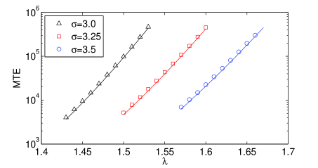
Figure 4: Mean time to extinction for the stochastic Allee population model with an initial population given by $X_{2}$. The curves are found using the analytical approximation given by Eq. (11), and the symbols represent the corresponding numerical simulation results. The numerical results are based on 10,000 realizations with $\mu=0.2$ and $K=100$ as $\sigma$ and $\lambda$ are varied.

The analytical MTE is found using Eq. (11) and is confirmed using numerical simulations. A Monte Carlo algorithm (Gillespie, 1976) is used to evolve the population in time, and Fig. 3 shows an example of one stochastic realization. Figure 3 shows that the population persists for a very long time near the $X_{2}$ state (deterministically stable) but eventually the noise causes the population to go extinct. By numerically computing thousands of stochastic realizations and the associated extinction times, one can calculate the MTE. Figure 4 shows the comparison between the analytical and the numerical mean time to extinction as a function of $\lambda$ for various choices of $\sigma$. Each numerical result is based on 10,000 Monte Carlo simulations, and the agreement is excellent.

4 Extinction with Cycling

In the previous section, we saw that there were three steady states associated with the deterministic Allee model, two of which were stable (a non-zero carrying capacity and the extinct state) and one of which was unstable (a threshold state). Additionally, we saw that for the stochastic Allee model, the population fluctuated for a long period of time about one of the deterministically stable states before stochastically switching to the extinct state. There are many models whose deterministic mean-field equation has multiple non-zero stable steady states. In these cases, the population can switch between these different population levels repeatedly before going extinct. As an example, Fig. 5 shows a flowchart with stable states located at $x_{0}$ (the extinct state), $x_{2}$, and $x_{4}$. In this example, there are two unstable states at $x_{1}$ and $x_{3}$ (not shown). One can see from Fig. 5 that the population may stochastically cycle multiple times from $x_{2}$ to $x_{4}$ and back to $x_{2}$ before eventually transitioning to the $x_{0}$ extinct state. In this section, we investigate a population’s MTE when cycling occurs as a pre-extinction event. Furthermore, we derive a new analytical result for the mean time to extinction by considering the probability of stochastic switching events and their associated transition times. This is one of the main results of this article.

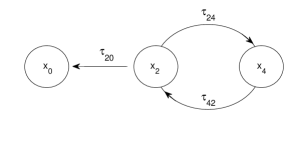
Figure 5: Flowchart for a model whose deterministic mean-field equation has multiple non-zero stable steady states. The stable states are located at $x_{0}$ (the extinct state), $x_{2}$, and $x_{4}$. There are two unstable states at $x_{1}$ and $x_{3}$ (not shown). The population may stochastically cycle multiple times from $x_{2}$ to $x_{4}$ and back to $x_{2}$ before eventually transitioning to the $x_{0}$ extinct state.

4.1 An example of population cycling

It is straightforward to extend the Allee model of Sec. 3 to a model whose deterministic mean-field equation is a quintic polynomial with five steady states, three of which are stable. The stochastic version of this new model will exhibit pre-extinction cycling as previously discussed. This stochastic population model is represented by the following transition processes and associated rates $W(X;r)$.

Transition	W(X;r)
${\displaystyle X\overset{\mu}{\longrightarrow}\varnothing}$	$\mu X$,
$2X\overset{\lambda/K}{\longrightarrow}3X$	$\lambda\frac{X(X-1)}{2K}$,
$3X\overset{\sigma/K^{2}}{\longrightarrow}2X$	$\sigma\frac{X(X-1)(X-2)}{6K^{2}}$,
$4X\overset{\alpha/K^{3}}{\longrightarrow}5X$	$\alpha\frac{X(X-1)(X-2)(X-3)}{24K^{3}}$,
$5X\overset{\beta/K^{4}}{\longrightarrow}4X$	$\beta\frac{X(X-1)(X-2)(X-3)(X-4)}{120K^{4}}$.

The first three events are the same as found in the stochastic Allee model in Sec. 3 and allow for fluctuations around a population level before going extinct. The two new events with their associated positive ($\alpha$) and negative ($\beta$) growth rates allow for fluctuations around a second population level as well as cycling between the two population levels before going extinct.

As described in Sec. 2, the transition processes and their associated rates are used to formulate the master equation given by Eq. (1). Note that the transitions are single-step because the increment $r$ only takes on the values of $\pm 1$. Therefore, the scaled transition rates $w_{r}(x)$ and $u_{r}(x)$ in Eq. (2) are given as

$$\begin{array}[]{lll}w_{1}(x)=\frac{\lambda x^{2}}{2}+\frac{\alpha x^{4}}{24},&{}{}{}{}{}{}&w_{-1}(x)=\mu x+\frac{\sigma x^{3}}{6}+{\frac{\beta x^{5}}{120}},\\ &&\\ u_{1}(x)=-\frac{\lambda x}{2}-\frac{\alpha x^{3}}{4},&{}{}{}{}{}{}&u_{-1}(x)=-\frac{\sigma x^{2}}{2}-\frac{\beta x^{4}}{12}.\\ \end{array}$$ (19)

Substitution of Eq. (19) into Eq. (4) leads to the following Hamiltonian:

$$\mathcal{H}(x,p)=\left(\frac{\lambda x^{2}}{2}+\frac{\alpha x^{4}}{24}\right)\left({e^{p}}-1\right)+\left(\mu x+\frac{\sigma x^{3}}{6}+{\frac{\beta x^{5}}{120}}\right)\left({e^{-p}}-1\right).$$ (20)

Taking derivatives of Eq. (20) with respect to $p$ and $x$ (Eq. (6)) lead to the following system of Hamilton’s equations:

$$\dot{x} = \left(\frac{\lambda x^{2}}{2}+\frac{\alpha x^{4}}{24}\right){e^{p}}-\left(\mu x+\frac{\sigma x^{3}}{6}+{\frac{\beta x^{5}}{120}}\right){e^{-p}},$$ (21)

$$\dot{p} = -\left(\lambda x+\frac{\alpha x^{3}}{6}\right)\left({e^{p}}-1\right)-\left(\mu+\frac{\sigma x^{2}}{2}+\frac{\beta x^{4}}{24}\right)\left({e^{-p}}-1\right).$$ (22)

Once again, by setting the Hamiltonian in Eq. (20) equal to zero and solving for $p$ and $x$ it is possible to find the zero-energy phase trajectories to be $x=0$, the extinction line; $p=0$, the deterministic line and

$$p_{opt}(x)=\ln{\left({\frac{120\mu+20\sigma x^{2}+\beta x^{4}}{5x\left(\alpha x^{2}+12\lambda\right)}}\right)},$$ (23)

the optimal path to extinction. The $p=0$ and $p_{opt}(x)$ solutions found using Eq. (20) are shown in Fig. 6. Using Eq. (7) we can recover the deterministic mean-field equation by substituting $p=0$ into Eq. (21) to obtain

$$\dot{x}=-\frac{\beta}{120}x^{5}+\frac{\alpha}{24}x^{4}-\frac{\sigma}{6}x^{3}+\frac{\lambda}{2}x^{2}-\mu x.$$ (24)

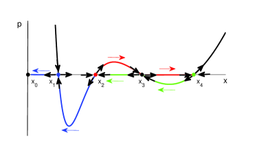
Figure 6: Zero-energy trajectories of the Hamiltonian for the stochastic Allee population model given by Eq. (20). The optimal path of transitioning from one state to another is given by $p=0$ or $p_{opt}(x)$ (Eq. (23)). A cycling path (red and green) consists of the heteroclinic trajectory connecting $x_{2}$ to $x_{3}$ (red) and the $p=0$ line from $x_{3}$ to $x_{4}$ (red), followed by the heteroclinic trajectory connecting $x_{4}$ to $x_{3}$ (green) and the $p=0$ line from $x_{3}$ to $x_{2}$ (green). The optimal path to extinction consists of the heteroclinic trajectory from $x_{2}$ to $x_{1}$ (blue) and the $p=0$ line from $x_{1}$ to $x_{0}$ (blue).

Equation (24) has five steady states: the extinct state $x_{0}=0$, and four non-zero states, two of which are stable and two of which are unstable. In the deterministic model given by Eq. (24), $x_{1}$ and $x_{3}$ are unstable states. For initial conditions whose value lies between $x_{1}$ and $x_{2}$, the deterministic solution will increase to $x_{2}$, which is a stable steady state. For initial conditions whose value is less than $x_{1}$, the deterministic solution will decrease to the stable extinct steady state $x_{0}$. Similarly, when initial conditions have a value between $x_{3}$ and $x_{4}$, the deterministic solution will increase to $x_{4}$, which is a stable steady state. When initial conditions have a value between $x_{3}$ and $x_{2}$, the deterministic solution will decrease to the stable steady state $x_{2}$.

As we have already seen in the previous section, the inclusion of intrinsic noise in the model leads to the steady states of Hamilton’s equations being two-dimensional with both $p$ and $x$ components. Furthermore, the steady states of the stochastic cycling model will be saddle points, as seen in Fig. 6. Figure 6 shows that starting from $x_{2}$ there is a choice to be made: 1) the population could go extinct by traveling along the blue path, which is the heteroclinic trajectory connecting $x_{2}$ to $x_{1}$, followed by traveling along the $p=0$ line from $x_{1}$ to the extinct state $x_{0}$, much like what happens in the stochastic Allee model; or 2) the population could cycle to $x_{4}$ and back by traveling along the red path and then the green path, which includes two stochastic escapes. First, the population travels along the heteroclinic trajectory connecting $x_{2}$ to $x_{3}$, followed by traveling along the $p=0$ line from $x_{3}$ to $x_{4}$. After fluctuating for some time about $x_{4}$, the population returns to $x_{2}$ by traveling along the heteroclinic trajectory from $x_{4}$ to $x_{3}$, followed by traveling along the $p=0$ line from $x_{3}$ to $x_{2}$.

A Monte Carlo algorithm (Gillespie, 1976) is used to evolve the population in time, and Fig. 7 shows one stochastic realization. Figure 7 shows multiple cycling events between the $X_{2}$ and $X_{4}$ states (deterministically stable) before the population eventually goes extinct. By numerically simulating thousands of stochastic realizations, we can compute the mean time to extinction and compare the numerical result with an analytical result. We will now derive a novel analytical form for the mean time to extinction that will account for the additional pre-extinction cycling time that delays the actual extinction event.

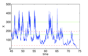
Figure 7: A single realization exhibiting cycling and extinction in the stochastic cycling population model. The non-zero deterministic stable states are shown by the green lines, while the deterministic unstable states are shown by the red dashed lines. The parameter values are $\mu=3.25$, $\alpha=0.465$, $\beta=0.048$, $\lambda=3.96$, $\sigma=1.905$, and $K=14$.

4.2 Approximating the extinction time

Consider the model whose flowchart is given in Fig. 5. The deterministic mean-field equation for this model has multiple non-zero stable steady states located at $x_{2}$ and $x_{4}$ along with the extinct state located at $x_{0}$. In the corresponding stochastic model, the population may stochastically cycle multiple times from $x_{2}$ to $x_{4}$ and back to $x_{2}$ before eventually transitioning to the extinct state $x_{0}$. It is important to note that in this example it is not possible to experience unlimited population growth (Meerson and Sasorov, 2008), and eventually the population will go extinct.

If the system is located at $x_{2}$, there are only two options for a stochastic switch: 1) the population can go to the extinct state $x_{0}$, or 2) the population can switch to $x_{4}$. Since the population will eventually go extinct, it follows that any stochastic switch from $x_{2}$ to $x_{4}$ must result in a following switch from $x_{4}$ back to $x_{2}$ at some later time. Furthermore, the population may cycle from $x_{2}$ to $x_{4}$ and back to $x_{2}$ any number of times before the population eventually goes extinct by switching from $x_{2}$ to the absorbing extinct state $x_{0}$.

In isolation, the probability of the population switching from $x_{2}$ to $x_{0}$ can be approximated as $1/\tau_{20}$. Similarly, the probability of the population switching from $x_{2}$ to $x_{4}$ can be approximated by $1/\tau_{24}$. Recall that both $\tau_{20}$ and $\tau_{24}$ can be approximated using Eq. (11). However, in the cycling model, these switches do not occur in isolation. Rather, there is a “competition” as to which switch will happen first. Therefore, we must compute the probability of one switch occurring before the other. The probability of the population switching from $x_{2}$ to $x_{0}$ before switching from $x_{2}$ to $x_{4}$ is

$$\mathcal{P}_{20}=\frac{\frac{1}{\tau_{20}}}{\frac{1}{\tau_{20}}+\frac{1}{\tau_{24}}}=\frac{\tau_{24}}{\tau_{20}+\tau_{24}}.$$ (25)

Note that we will use the general notation $\mathcal{P}_{ij}$ to denote the probability that an escape from $x_{i}$ to $x_{j}$ happens first. Also, $\mathcal{P}_{24}=1-\mathcal{P}_{20}$ because there are only two switching options.

To find the MTE, we use a probabilistic argument whereby the probability of a given event (immediate extinction, one cycle followed by extinction, two cycles followed by extinction, etc.) is weighted by the approximate time of each event. Each transition time is found using Eq. (11), and it should be noted that each probability term is written in terms of these approximate transition times (e.g. Eq. (25)). The MTE thus becomes the sum of the expected times for all possible number of cycles to occur and the final escape from $x_{2}$ to $x_{0}$:

$${\rm MTE} =\tau_{20}\mathcal{P}_{20}+\sum_{i=0}^{\infty}i(\tau_{24}+\tau_{42})(\mathcal{P}_{24})^{i}\mathcal{P}_{20}$$ (26a)

$$=\tau_{20}\mathcal{P}_{20}+\frac{(\tau_{24}+\tau_{42})\mathcal{P}_{24}}{\mathcal{P}_{20}}$$ (26b)

$$=\frac{\tau_{20}\tau_{24}}{\tau_{20}+\tau_{24}}+(\tau_{24}+\tau_{42})\frac{\tau_{20}}{\tau_{24}}.$$ (26c)

As in the stochastic Allee model, the analytical mean time to extinction for the stochastic cycling model can be confirmed using Monte Carlo simulations (Gillespie, 1976). Figure 8 shows the comparison between the analytical and numerical mean time to extinction as a function of $\lambda$ for various choices of carrying capacity $K$. Each numerical result is based on 5,000 Monte Carlo simulations, and the agreement is excellent. Note that the choice of $\lambda$ values for this example is limited by the quasi-stationarity requirement. However, in the following section, we continue the exploration of this example using control and show there is excellent agreement for MTE over several orders of magnitude of MTE.

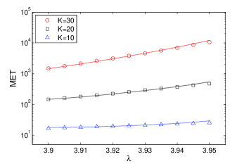
Figure 8: Mean time to extinction for the stochastic cycling population model with an initial population given by $X_{2}$. The solid curves are found using the analytical approximation given by Eq. (26c), and the symbols represent the corresponding numerical simulation results. The numerical results are based on 5,000 simulations with $\mu=3.307$, $\alpha=0.458$, $\beta=0.047$, and $\sigma=1.8874$ as $K$ and $\lambda$ are varied.

5 Speeding up Extinction

The previous section presents a way to find the MTE in a population model with cycling so that extinction is delayed. Often the MTE is of interest in the study of population dynamics because either longevity or quick extinction has value. The population studied in this section should be thought of as pests, and a short MTE should be considered ideal. The control method we model removes individuals at a particular frequency $\nu$. This population will have all the same demographic events that were seen in the cycling population model, and will have the following event in addition:

Transition	W(X;r)
${\displaystyle X\overset{\nu}{\longrightarrow}\varnothing}$	${\displaystyle\nu}$.

In an ecological context one might think of the control term as culling or quarantining.

The only change from the cycling model transition rates given by Eq. (19) is in the rate $w_{-1}$ which now has the form

$$w_{-1}(x)=\mu x+\frac{\sigma x^{3}}{6}+\frac{\beta x^{5}}{120}+\frac{\nu}{K}.$$ (27)

Using Eq. (4), the modified Hamiltonian will be

$$\mathcal{H}(x,p)=\left(\frac{\alpha x^{4}}{24}+\frac{\lambda x^{2}}{2}\right)(e^{p}-1)+\left(\mu x+\frac{\sigma x^{3}}{6}+\frac{\beta x^{5}}{120}+\frac{\nu}{K}\right)(e^{-p}-1).$$ (28)

To quantify the change in the MTE as a function of $\nu$, we use Eq. (26c) and the modified Hamiltonian given by Eq. (28).

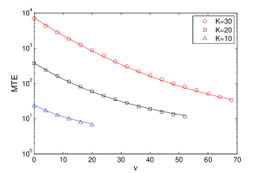
Figure 9: Mean time to extinction for the stochastic cycling population model using control with an initial population given by $X_{2}$. The solid curves are found using the analytical approximation. The symbols represent the corresponding numerical simulation results. The numerical results are based on 5,000 simulations with $\mu=3.307$, $\alpha=0.458$, $\beta=0.047$, $\lambda=3.94$, and $\sigma=1.8874$ as $K$ and $\nu$ are varied.

The analytical mean time to extinction for the stochastic cycling model with control can be confirmed using Monte Carlo simulations (Gillespie, 1976). Figure 9 extends the examples from Fig. 8 by comparing the analytical and numerical mean time to extinction as a function of $\nu$. Each numerical result is based on 5,000 Monte Carlo simulations, and the agreement is excellent over several orders of magnitude of MTE. As expected, when more individuals are removed from the population the MTE decreases.

6 Conclusions and Discussion

In this article, we have considered stochastic population models where the intrinsic or demographic noise eventually causes the population to go extinct. For models that exhibit stochastic cycling between two states, we described the optimal path to extinction and an analytical method to approximate the mean time to extinction. We used a probabilistic argument to understand the pre-extinction dynamics that delay the extinction event.

These results for the MTE can be extended to the general case of a system with $2n+1$ steady states (($n\in\mathbb{N}$), $n>1$), with the possibility of $n-1$ cycles. We assume there are $n+1$ deterministically stable steady states $\{X_{0},X_{2},X_{4},\ldots,X_{2n}\}$ alternating with deterministically unstable steady states, and that $X_{0}$ is an absorbing extinct state. For a system starting at $X_{2}$,

$$MTE=\tau_{20}\mathcal{P}_{20}+\sum_{i=1}^{n-1}\left[\left(\tau_{2i,2i+2}+\tau_{2i+2,2i}\mathcal{P}_{2i+2,2i}\right)\prod_{k=1}^{i}\frac{\mathcal{P}_{2k,2k+2}}{\mathcal{P}_{2k,2k-2}}\right].$$ (29)

Note that when situated at $X_{2n}$, the stable steady state furthest away from the extinct state, then there is no choice of switching. The only possible switch is from $X_{2n}$ to $X_{2n-2}$, and therefore $\mathcal{P}_{2n,2n-2}=1$. This result can also be extended to find the MTE when the system starts at any of the other deterministically stable steady states. Consider an initial condition $X_{2k}$ for $k<n$. One would need to find the mean time for each escape in the sequence $X_{2k},X_{2k-2},\ldots,X_{0}$. For example, starting at $X_{2k}$ would reduce the problem to the subsystem of deterministically stable steady states $\{X_{2k-2},X_{2k},\ldots,X_{2n}\}$ for which Eq. (29) would approximate the mean escape time to $X_{k-2}$. Repeating this procedure leftward and taking the sum of these mean escape times would result in the total MTE.

Lastly, a control method was introduced to the stochastic cycling population model. The mean time to extinction was calculated analytically and was shown to agree well with numerical Monte Carlo simulations. It was shown that the mean time to extinction decreases monotonically with an increased removal program. From an ecological perspective it is important to work towards a quantitative understanding of how control methods (e.g. bio-control agents, culling programs, quarantine programs, or hunting allowances) may affect the longevity of a population.