Average Lorentz Self-Force From Electric Field Lines

Abstract

We generalize the derivation of electromagnetic fields of a charged particle moving with a constant accelerationsingal to a variable acceleration (piecewise constants) over a small finite time interval using Coulomb’s law, relativistic transformations of electromagnetic fields and Thomson’s constructionthmsn . We derive the average Lorentz self-force for a charged particle in arbitrary non-relativistic motion via averaging the fields at retarded time.

I Introduction

The electromagnetic fieldssingal of a charged particle moving with a constant acceleration are obtained exploiting Coulomb force, relativistic transformations of electromagnetic fields and Thomson’s constructionthmsn . The derivation of the fields for an accelerated charge is carried out in the instantaneous rest frame. The geometry of the Thomson’s construction makes it evident that fields pick up the transverse components proportional to acceleration in addition to the radial components. The electromagnetic fields so obtained turn out exactly the same as those obtained via Lienard-Weichert potentials. This method is mathematically simpler than the usual methodjack1 of computing the electromagnetic fields which involves rather cumbersome calculations.
However, the one downside to this method is that it is not sufficient to calculate the radiation reaction force. The derivation of radiation reaction involves non-uniform acceleration of the charged particle.
In this paper, we address the question as to how to calculate the EM fields for a charged particle moving with a variable acceleration (piecewise constants) over a small finite time interval $\Delta t$ using relativistic transformations of fields $\vec{E}$ and $\vec{B}$, Coulomb field of a stationary charge as well as Thomson’s construction. Consider a charge moving with piecewise different constant accelerations in time interval $\Delta t$. The charge moving with piecewise $N$(say) different constant accelerations over time interval $\Delta t$ enables us to use the relativistic transformations of fields $\vec{E}$ and $\vec{B}$ of a uniformly moving charge through $N$ small time sub-intervals $\Delta t/N$(say). The electromagnetic fields at some space and time points are obtained by time-averaging out the fields stemming from the piecewise $N$ different constantly accelerated motions of the charge through $N$ temporal sub-intervals $\Delta t/N$.
A charged particle moving with non-uniform acceleration radiates. A radiating charged particle experiences a force which acts on the charge particle and is called as self-force. The Lorentz self-force (jack1, , p. 753) arising due to a point charge conceived as a uniformly charged spherical shell of radius $s$ is given by

$$\vec{F}_{self}=-\frac{2}{3}\frac{{q^{2}}}{{4\pi\varepsilon_{0}c^{2}s}}\dot{\vec{v}}(t)+\frac{2}{3}\frac{{q^{2}}}{{4\pi\varepsilon_{0}c^{3}}}\ddot{\vec{v}}(t)+O(s)~{}~{}\textup{with}~{}~{}|\vec{s}|=s$$ (1)

where,

• the quantity $\frac{2}{3}\frac{{q^{2}}}{{4\pi\varepsilon_{0}c^{2}s}}$ in the first term stands for electromagnetic mass and becomes divergent as $s\to 0^{+}$,

• the second term represents the radiation reaction and is independent of the dimension of the charge distribution and

• the third term corresponds to the first finite size correction and is proportional to the radius of the shell $s$.

It is plausible to expect that the piecewise $N$ different constantly accelerated motions of the charge through $N$ temporal sub-intervals $\Delta t/N$ could give rise to the average self-force. We derive the average Lorentz self-force for the charged particle in arbitrary non-relativistic motion via averaging the said retarded fieldshaque .

II Preliminary

In this section, we shall briefly discuss about the relativistic transformations of the fields and Thomson’s constructionthmsn . We shall further discuss and summarize the results on the electromagnetic field of a constantly accelerated charge in the instantaneous rest framesingal and self-forcehaque .

II.1 Relativistic Transformations of $\vec{E}$ and $\vec{B}$ of a Uniformly Moving Charge

Let us consider two frames $S$ and $S^{\prime}$. Let $S^{\prime}$ is moving with constant velocity $\vec{v}=\vec{\beta}c$ relative to $S$. Suppose a particle of charge $q$ moves with a velocity $\vec{v}$ relative to $S$. The charged particle would thus appear to be at rest with respect to the system $S^{\prime}$.
The electric $\vec{E}$ and magnetic fieldsdjg $\vec{B}$ of the charged particle in frame $S$ is related to the electric $\vec{E}^{\prime}$ and magnetic fields $\vec{B}^{\prime}$ of the charged particle in the frame $S^{\prime}$ as follows:

$$\vec{E} = \vec{E^{\prime}}_{\parallel}+\gamma[\vec{E^{\prime}}_{\perp}-\vec{\beta}\times\vec{B^{\prime}}]~{},~{}\vec{B}=\vec{B^{\prime}}_{\parallel}+\gamma[\vec{B^{\prime}}_{\perp}+\vec{\beta}\times\vec{E^{\prime}}]$$

$$\vec{E}^{\prime} = \vec{E}_{\parallel}+\gamma[\vec{E}_{\perp}+\vec{\beta}\times\vec{B}]~{},~{}\vec{B}^{\prime}=\vec{B}_{\parallel}+\gamma[\vec{B}_{\perp}-\vec{\beta}\times\vec{E}]$$ (2)

In case, the charged particle moves with non-relativistic speed $|\vec{\beta}|<<1~{}i.e.~{}\gamma\to 1$, $\vec{E}$ and $\vec{B}$ field transformations simplify to yield:

$$\vec{E} = \vec{E^{\prime}}-\vec{\beta}\times\vec{B^{\prime}}~{},~{}\vec{B}=\vec{B^{\prime}}+\vec{\beta}\times\vec{E^{\prime}}$$ (3)

$$\vec{E}^{\prime} = \vec{E}+\vec{\beta}\times\vec{B}~{},~{}\vec{B}^{\prime}=\vec{B}-\vec{\beta}\times\vec{E}$$ (4)

In $S^{\prime}$ frame, field is purely electric as the charge is at rest with respect to the system $S^{\prime}$. Therefore,

$$\vec{B^{\prime}}=0,\vec{E}=\vec{E^{\prime}}~{}\textup{and}~{}\vec{B}=\vec{\beta}\times\vec{E^{\prime}}$$ (5)

Now, suppose that the charged particle is moving along the Z-axis($\theta=0$) i.e. $\vec{\beta}=\beta\hat{z}$, then in the spherical polar coordinates $(R,\theta,\phi)$, we have

$$\vec{E} = E_{R}\hat{R}=\frac{e^{2}}{R^{2}}\hat{R}$$ (6)

$$\vec{E^{\prime}} = E_{R}^{\prime}\hat{R^{\prime}}=\frac{e^{2}}{R^{\prime 2}}\hat{R^{\prime}}$$ (7)

$$\vec{B} = \vec{\beta}\times\vec{E^{\prime}}=\vec{\beta}\times\vec{E}=B_{\phi}\hat{\phi}=\frac{e\beta\sin\theta}{R^{2}}\hat{\phi}$$ (8)

Now, $\vec{E}=\vec{E^{\prime}}$ implies that $R=R^{\prime}$ where $R$ is the distance between the field point and the location of the charge in the frame $S$.

II.2 Thomson’s Construction

Consider a charged particle, initially moving with a constant velocity $\vec{v}_{I},$ suffers a change in velocity after the time interval $(0,\tau)$ to a constant velocity $\vec{v}_{F}$. Suppose the charged particle undergoes an acceleration to a small velocity $\Delta\vec{v}$ ($\Delta v<<c$) for the short time $\tau$. Arguments due to Thompson, regarding the resulting field distribution in terms of the electric field lines after time $t=T$, attached to the accelerated charge are summarized as follows:

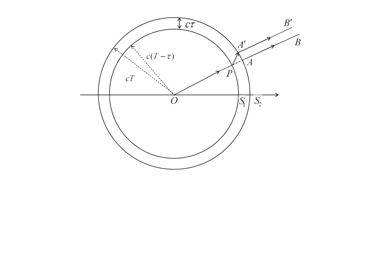
Figure 1: Electric field line as per Thomson’s construction exhibiting the ’kink’ in between the spherical surfaces $S_{1}$ and $S_{2}$ corresponding to the acceleration of the charge.

• For any time $t<0$, fields are that of the charge moving with constant velocity $\vec{v}_{I}$. The electric field lines will emanate radially outward from the charge in all possible directions. The information pertaining to the change in motion (acceleration) can’t reach outside a sphere of radius $R=cT$.

• For any time $0<t<\tau$, fields are that of the charge undergoing acceleration. The electric field lines will admit distortions in the form of a kink in a region between the two spheres $S_{1}$ and $S_{2}$ (as shown in FIG.1 ) in order to preserve the continuity of the field lines. Thus, the fields would now begin to pick up the tangential component in addition to the radial one. The information pertaining to the change in motion is confined in the spatial region $cT<R<c(T-\tau)$.

• For any time $t>\tau$ fields are that of the charge moving with constant velocity $\vec{v}_{F}.$ The electric field lines will emanate radially outward from the charge in all possible directions. The information pertaining to the change in motion can’t reach inside a sphere of radius $R=c(T-\tau)$.

II.3 Electromagnetic Field of the Constantly Accelerated Chargesingal

Consider a charged particle moving in a lab-frame $S$. Suppose the charge is moving with a constant initial velocity $\vec{v}_{0}$. Let the charge be uniformly accelerated $\vec{a}$ for a short time interval ($-\Delta t/2,\Delta t/2$) to a velocity $\Delta\vec{v}(\Delta v<<c)$ so that its velocity become $\vec{v}_{1}$ (constant). The velocity of the charge at $t=0$ is $\vec{v}=(\vec{v}_{0}+\vec{v}_{1})/2$.
Consider a (instantaneous rest) frame $S^{\prime}$ moving with velocity $\vec{v}=(\vec{v}_{0}+\vec{v}_{1})/2$ relative to frame $S$. The initial and final velocities say $\vec{v^{\prime}}_{0}$ and $\vec{v^{\prime}}_{1}$ respectively of the charged particle relative to frame $S^{\prime}$ turn out equal and opposite $\vec{v^{\prime}}_{1}=-\vec{v^{\prime}}_{0}\equiv\vec{v^{\prime}}~{}(say)$. For convenience, $S^{\prime}$ could be rotated (rotation can be undone at the end) so that the charge motion is along the horizontal axis.
Suppose the charge be instantaneously at rest at $O^{\prime}$ at $t^{\prime}=0$. The charge moves a distance $a^{\prime}\Delta t^{\prime 2}/8$ towards $O^{\prime}$ and then gets back in duration $\Delta t^{\prime}$. To the first order in $\Delta t^{\prime},$ charge could be assumed to be practically at rest at $O^{\prime}$. Consider the fields of the charge at time $T^{\prime}>>\Delta t^{\prime}$. Let $O^{\prime}_{1}$ and $O^{\prime}_{2}$ (for $N=1$) be the positions of the charge at $T^{\prime}-\Delta t^{\prime}/2$ and $T^{\prime}+\Delta t^{\prime}/2$ respectively. The electric field in the regions $c(T^{\prime}+\Delta t^{\prime}/2)<r^{\prime}<c(T^{\prime}-\Delta t^{\prime}/2)$ would be in the radial direction from the points $O^{\prime}_{1}$ and $O^{\prime}_{2}$. We wish to calculate the electric field in the region $c(T^{\prime}-\Delta t^{\prime}/2)<\Delta r^{\prime}<c(T^{\prime}+\Delta t^{\prime}/2)$ which possesses the information of the change in motion of the charge.
Geometrically, it is obvious from the Thomson’s construction (for $N=1$), that the field now picks up both the radial ($E^{\prime}_{r^{\prime}}$) as well as the transverse components ($E^{\prime}_{\theta^{\prime}}$) both at $A$ and $B$. The spatial variation in the transverse components of electric field over a distance $\Delta r^{\prime}$ from $A$ to $B$ turns out,

$$\frac{{\partial E^{\prime}_{\theta^{\prime}}}}{{\partial r^{\prime}}}=\frac{{-e}}{c}\frac{{\dot{\beta}^{\prime}\sin\theta^{\prime}}}{{r^{\prime 2}}}$$ (9)

The formal solution of (9) at $P(r^{\prime},t)$ assuming that field falls to zero as $r^{\prime}\to\infty$ leads to

$$E^{\prime}_{\theta^{\prime}}=\frac{{e\dot{\beta}^{\prime}\sin\theta^{\prime}}}{{cr^{\prime}}}$$ (10)

The total electric field at $P(r^{\prime},t)$ could be written as:

$$\vec{E}^{\prime}=\frac{q}{r^{\prime 2}}\hat{r^{\prime}}+\frac{q}{c^{2}}\frac{\vec{r^{\prime}}\times(\vec{r^{\prime}}\times\dot{\vec{v^{\prime}}})}{r^{\prime}}$$ (11)

The transformation of the field from $S^{\prime}$ to $S$ yields:

$$\vec{E}=q\frac{\hat{r}-\vec{\beta}}{r^{2}\gamma^{2}(1-\hat{r}\cdot\vec{\beta})^{3}}+\frac{q}{c}\frac{\hat{r}\times\{(\hat{r}-\vec{\beta})\times\dot{\vec{\beta}}\}}{r(1-\hat{r}\cdot\vec{\beta})^{3}}$$ (12)

In the non-relativistic case ($\frac{v}{c}<<1~{}i.e.~{}\gamma\rightarrow 1$), the expression for $\vec{E}$ takes the form:

$$\vec{E}=q\frac{\hat{r}-\vec{\beta}}{r^{2}(1-\hat{r}\cdot\vec{\beta})^{3}}+\frac{q}{c}\frac{\hat{r}\times\{(\hat{r}-\vec{\beta})\times\dot{\vec{\beta}}\}}{r(1-\hat{r}\cdot\vec{\beta})^{3}}$$ (13)

II.4 Results of The Self-forcehaque

A simple derivation of the self-forcehaque based on the consideration that the averaged value of the field in the suitably small closed region surrounding the point charge is the value of the field under consideration at the position of the point charge is carried out in detail.
The self-force is defined as:

$$\vec{F}_{Self}(\vec{r},t)=q\mathop{Lim}\limits_{s\to 0^{+}}\overline{\vec{E}}(\vec{r},t)=q\vec{E}_{Self}(\vec{r},t)$$ (14)

where $\overline{\vec{E}}(\vec{r},t))$ is average field over the surface of a spherical shell of radius $s$ and the field ${\vec{E}}(\vec{r},t)$ depends upon the position and motion of the charge particle at the retarded time. Using the field due to an accelerated charged particle (in the limit $v/c\to 0$), the self force turns out:

$$\vec{F}_{Self}(\vec{r},t)=-\frac{2}{3}\frac{q^{2}}{4\pi\epsilon_{0}c^{2}}\left(\mathop{Lim}\limits_{s\to 0^{+}}\frac{\vec{a}(t-s/c)}{s}\right)$$ (15)

III Calculation of Average Electric Field

Consider a charge moving with an initial velocity $\vec{v}_{0}$ in the lab frame $S$. Suppose it undergoes accelerations from $-\Delta t/2$ to $\Delta t/2$. We consider that the acceleration in the time interval $\Delta t$ is not continuous but rather consists of a series of a finite number of different piecewise constant accelerations. Let us divide the total time interval $\Delta t$ into a large number $2N(N\geq 2)$ of sub-intervals. Suppose all the odd and even sub-intervals are of lengths $(1-\varepsilon)\Delta t/N$ and $\varepsilon\Delta t/N$ respectively. We consider that the charge undergoes nonzero constant accelerations in the odd sub-intervals accompanied by nonzero constant velocities in the even sub-intervals. Accelerations {$\vec{a_{i}}(\tau_{i}):i=1,3,5,...,2N-1$} and velocities {$\vec{v}_{i}(t):i=0,2,...,2N$} are defined as:

$$\vec{a}_{i}(\tau_{i}) = \left\{\begin{array}[]{l}\vec{a}_{i}\theta(\tau_{i}-t_{i-1})\theta(t_{i}-\tau_{i})~{};~{}i=1,3,5,...,2N-1\\ 0,{\rm{}}(t_{i}<\tau_{i}<t_{i+1})~{};~{}i=0,2,...,2N\\ \end{array}\right.$$ (18)

$$\vec{v}_{i+1}(t) = \vec{v}_{i}+\int^{\frac{\Delta t}{2}}_{-\frac{\Delta t}{2}}\vec{a}_{i+1}(\tau_{i})d\tau_{i}~{};~{}i=0,2,...,2N$$ (19)

where,

$$t_{i}=\left\{\begin{array}[]{l}\left({-\frac{1}{2}+\frac{i}{{2N}}}\right)\Delta t~{};~{}i=0,2,...,2N.\\ \left({-\frac{1}{2}+\frac{{i+1-2\varepsilon}}{{2N}}}\right)\Delta t~{};~{}i=1,3,5,...,2N-1.\\ \end{array}\right.$$

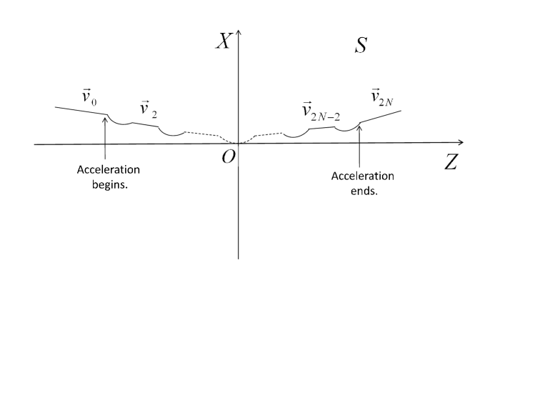
Figure 2: A schematic of the motion of a piecewise constantly accelerated charge.

The charge undergoes through various different piecewise constant accelerations in the time interval $\Delta t$. In order to determine the EM fields of an accelerated charge over $\Delta t$, we require as many instantaneous rest-frames as that of the different constant accelerations. These instantaneous rest-frames could be obtained by appropriate boosts. Let us consider the ith instantaneous rest-frame {$S^{\prime}_{i}:i=1,3,5,...,2N-1$} moving with velocity {$\vec{v}_{S^{\prime}_{i}}=(\vec{v}_{i}+\vec{v}_{i+1})/2:i=1,3,5,...,2N-1$}. We assume that $|\vec{v}_{i+1}-\vec{v}_{i}|<<c$. Suppose the charged particle appears to be instantaneuosly at rest at $(\frac{t^{\prime}_{i}+t^{\prime}_{i+1}}{2};~{}i=0,2,...,2N-2)$ where

$$t^{\prime}_{i}=\left\{\begin{array}[]{l}\left({-\frac{1}{2}+\frac{i}{{2N}}}\right)\Delta t^{\prime}~{};~{}i=0,2,...,2N.\\ \left({-\frac{1}{2}+\frac{{i+1-2\varepsilon}}{{2N}}}\right)\Delta t^{\prime}~{};~{}i=1,3,5,...,2N-1.\\ \end{array}\right.$$

Thomson’s construction for $N=2$ is shown in FIG.4. In the frame $S^{\prime}_{i}$, the corresponding transformed velocities $\vec{v}^{\prime}_{i-1}$ and $\vec{v}^{\prime}_{i+1}$ are given by:

$$\vec{v}^{\prime}_{i+1}=-\vec{v}^{\prime}_{i-1}=\vec{v}^{\prime}_{i}~{}(\textup{say})$$ (20)

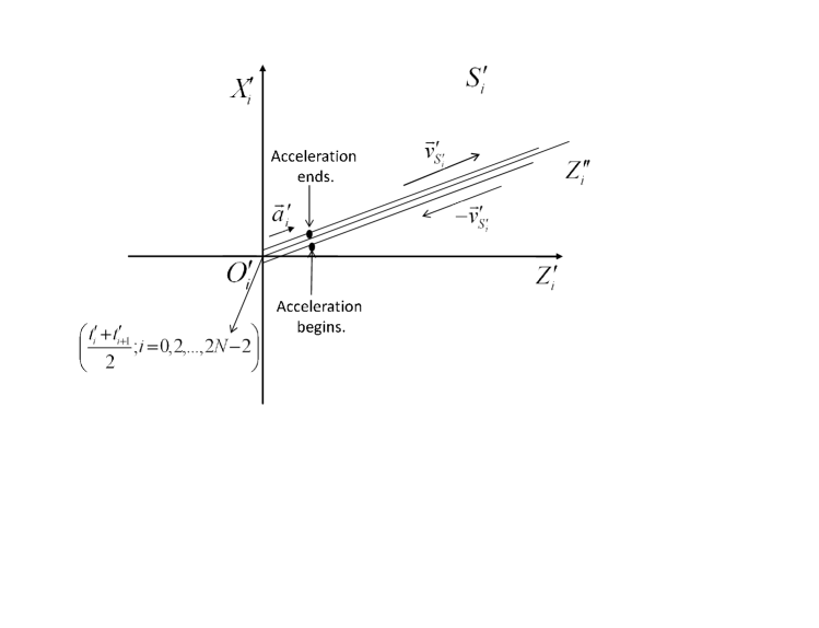
Figure 3: Motion of a piecewise constantly accelerated charge as observed in the instantaneous rest frames $S^{\prime}_{i}$.

The acceleration in $S^{\prime}_{i}$ reads:

$$\vec{a}^{\prime}_{i}=\frac{2\vec{v}^{\prime}_{i}}{(1-\varepsilon)\Delta t^{\prime}/N}$$ (21)

Without any loss of generality, we take the orientation of $S^{\prime}_{i}$ such that motion happens along $Z^{\prime}_{i}$. The calculation of $E^{\prime}_{i}$ in $S^{\prime}_{i}$ proceeds in a similar way to that in the section 3. The electric field $E^{\prime}_{i}$ at a later time $T^{\prime}>>\Delta t^{\prime}/N$ at $P$ is obtained as:

$$\vec{E}^{\prime}_{i}=\frac{q}{{r^{\prime 2}}}\hat{n}^{\prime}+\frac{q}{c}\frac{{\hat{n}^{\prime}\times\hat{n}^{\prime}\times\dot{\vec{\beta}}^{\prime}_{i}}}{r}$$

In the above expression, we have made use of

$$O^{\prime}_{i}B_{i}\approx O^{\prime}_{i+1}A_{i}\approx O^{\prime}P=r^{\prime};~{}i=1,2,...,N$$

as $\Delta{\theta^{\prime}}$ is small. Transformation of $\vec{E}^{\prime}_{i}$ to the lab frame $S$ for the non-relativistic velocity ($\vec{\beta}_{i}\to 0,\gamma\to 1$) yields:

$$\vec{E}_{i}=\frac{q}{{r^{2}}}\hat{n}+\frac{q}{c}\frac{{\hat{n}\times\hat{n}\times\dot{\vec{\beta}}_{i}}}{r}$$

where, $\hat{n}=\frac{\vec{r}}{r}$ and $\dot{\vec{\beta}}_{i}=\frac{{\vec{a}_{i}\left(\tau_{i}\right)}}{c}$. The quantities $\vec{r}$ and $\dot{\vec{\beta}}_{i}$ on the right hand side are evaluated at retarded time, $t_{R_{i}}=\tau_{i}-r/c$.

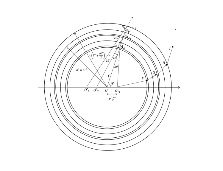
Figure 4: Electric field line $O_{3}FGHI$ as per Thomson’s construction exhibiting the ’kink’ in between the innermost and the outermost spherical surfaces corresponding to the accelerated motion of the charge. The thin annular region between the spherical surfaces belongs to the non-accelerated motion of the charge.

The electric field at $P$

$$\vec{E}_{i}=\left\{\begin{array}[]{l}\frac{q}{{r^{2}}}\hat{n}+\frac{q}{c}\frac{{\hat{n}\times\hat{n}\times\dot{\vec{\beta}}_{i}}}{r};~{}i=1,3,...,2N-1\\ \frac{q}{{r^{2}}}\hat{n};~{}i=0,2,...,2N.\\ \end{array}\right.$$

in fact consists of $N$ number of piecewise different values of $\vec{E}_{i}$ belonging to $2N-1$ sub-intervals over $\Delta t$. It is therefore plausible to consider the electric field at P in the vicinity of a point in time as the time-averaged value $\left\langle{\vec{E}}\right\rangle$ of the electric fields $\vec{E}_{i}$ for the entire time $\Delta t$. The time-averaged electric field is obtained as:

$$\left\langle{\vec{E}}\right\rangle = \frac{{\int\limits_{-\frac{{\Delta t}}{2}}^{\frac{{\Delta t}}{2}}{\sum\limits_{i=1}^{N}{\vec{E}_{i}dt}}}}{{\int\limits_{-\frac{{\Delta t}}{2}}^{\frac{{\Delta t}}{2}}{dt}}}=\frac{{\sum\limits_{i=1}^{N}{\left({\vec{E}_{2i-1}\frac{{1-\varepsilon}}{N}\Delta t+\vec{E}_{2i}\frac{\varepsilon}{N}\Delta t}\right)}}}{{\Delta t}}$$ (22)

$$= \frac{1}{N}\sum\limits_{i=1}^{N}{\left({\frac{q}{{r^{2}}}\hat{n}+\frac{q}{c}\frac{{\hat{n}\times\hat{n}\times\dot{\vec{\beta}}_{2i-1}}}{r}}\right)}-\frac{\varepsilon}{N}\sum\limits_{i=1}^{N}{\frac{q}{c}\frac{{\hat{n}\times\hat{n}\times\dot{\vec{\beta}}_{2i-1}}}{r}}$$

For $\varepsilon<<\frac{\Delta t}{N}$, we have:

$$\left\langle{\vec{E}}\right\rangle=\frac{q}{{r^{2}}}\hat{n}+\frac{q}{c}\frac{{\hat{n}\times\hat{n}\times\left\langle{\dot{\vec{\beta}}}\right\rangle}}{r}$$ (23)

where,

$$\left\langle{\dot{\vec{\beta}}}\right\rangle=\frac{{\frac{1}{c}\int\limits_{-\frac{{\Delta t}}{2}}^{\frac{{\Delta t}}{2}}{\vec{a}_{2i-1}(\tau_{2i-1})}d\tau_{2i-1}}}{{\Delta t}}=\frac{{\sum\limits_{i=1}^{N}{\frac{{\vec{a}_{2i-1}(\tau_{2i-1})}}{c}}}}{N}$$ (24)

IV Calculation of the Self force

The self force of a charge moving with arbitrary velocity, in general, contains acceleration and higher derivatives of acceleration as is especially obvious from equation (1). A charge moving with constant acceleration does not experience any radiation reaction as the term $\frac{2}{3}\frac{q^{2}}{4\pi\epsilon_{0}c^{3}}\ddot{\vec{v}}(t)$ vanishes.
In the case at hand, charge is moving with non-zero constant acceleration in the time interval $(1-\varepsilon)\Delta t/N$ whereas with zero acceleration in the time interval $\varepsilon\Delta t/N$. Therefore, the charge confined to these time intervals will not experience any radiation reaction force. However, over the interval $\Delta t$, the charge moving with various different constant accelerations would give rise to a net change in the acceleration $\Delta\vec{a}$ over $\Delta t$. This suggests that over the time $\Delta t$, $\Delta\vec{a}/\Delta t$ is no longer zero, and hence the charge must experience average radiation reaction. The average self-forcehaque may be defined as

$$\vec{F}_{Self}(\vec{r},t)=-\frac{2}{3}\frac{{q^{2}}}{{4\pi\varepsilon_{0}c^{2}}}\mathop{Lim}\limits_{s\to 0^{+}}\frac{{\left\langle{\vec{a}(\tau_{2i-1}-s/c)}\right\rangle}}{s}$$ (25)

where,

$$\vec{a}_{2i-1}(\tau_{2i-1}-s/c)=\vec{a}_{2i-1}\theta(\tau_{2i-1}-t_{2i-2}-s/c)\theta(t_{2i-1}-\tau_{2i-1}+s/c)$$

We can Taylor expand $\vec{a}_{2i-1}(\tau_{2i-1}-s/c)$ about $s/c$ so that,

$$\vec{a}_{2i-1}(\tau_{2i-1}-s/c)=\vec{a}_{2i-1}(\tau_{2i-1})-\frac{s}{c}\frac{d}{d\tau_{2i-1}}\vec{a}_{2i-1}(\tau_{2i-1})+O(s^{2})$$

The self force expression now becomes

$$\vec{F}_{Self}(\vec{r},t)=-\frac{2}{3}\frac{{q^{2}}}{{4\pi\varepsilon_{0}c^{2}}}\mathop{Lim}\limits_{s\to 0^{+}}\frac{\left\langle{\vec{a}(\tau_{2i-1})}\right\rangle}{s}+\frac{2}{3}\frac{{q^{2}}}{{4\pi\varepsilon_{0}c^{3}}}\left\langle{\dot{\vec{a}}(\tau_{2i-1})}\right\rangle$$

Since,

$$\theta(\tau_{2i-1}-t_{2i-2}-s/c)=\theta(\tau_{2i-1}-t_{2i-2})-\frac{s}{c}\delta(\tau_{2i-1}-t_{2i-2})+O(s^{2})$$

$$\theta(t_{2i-1}-\tau_{2i-1}+s/c)=\theta(t_{2i-1}-\tau_{2i-1})+\frac{s}{c}\delta(t_{2i-1}-\tau_{2i-1})$$

Therefore,

$$\sum\limits_{i=1}^{N}{\vec{a}_{2i-1}(\tau_{2i-1}-s/c)}=\sum\limits_{i=1}^{N}{\vec{a}_{2i-1}\theta(\tau_{2i-1}-t_{2i-2})\theta(t_{2i-1}-\tau_{2i-1})}$$

$$+\frac{s}{c}\sum\limits_{i=1}^{N}{\vec{a}_{2i-1}}\theta(t_{2i-1}-t_{2i-2})[\delta(t_{2i-1}-\tau_{2i-1})-\delta(\tau_{2i-1}-t_{2i-2})]+O(s^{2})$$

It is evident that $\vec{a}_{2i-1}(\tau_{2i-1}-s/c)$ turns out divergent at the temporal boundaries:

$$\tau_{2i-1}=t_{2i-1}~{}~{}\textup{or}~{}~{}\tau_{2i-1}=t_{2i-2}.$$

However, the time-averaged self force would render $\vec{a}_{2i-1}(\tau_{2i-1}-s/c)$ physically sensible. Moreover, in order to prevent this meaningless results, we assume that the transitions from non-zero constant acceleration to zero constant acceleration are smooth at the temporal boundaries (please see Appendix A for clarification). Such sort of meaningless results arise in models that involve step functions forcessch . Now,

$$\vec{F}_{Self}(\vec{r},t) = -\frac{2}{3}\frac{{q^{2}}}{{4\pi\varepsilon_{0}c^{2}s}}\left\langle{{\vec{a}}}\right\rangle$$ (26)

$$- \frac{2}{3}\frac{{q^{2}}}{{4\pi\varepsilon_{0}c^{3}}}\frac{1}{{\Delta t}}\int\limits_{-\frac{{\Delta t}}{2}}^{\frac{{\Delta t}}{2}}{\sum\limits_{i=1}^{N}{\vec{a}_{2i-1}[\delta(t_{2i-1}-\tau_{2i-1})-\delta(\tau_{2i-1}-t_{2i-2})]d\tau_{2i-1}}}$$

$$= -\frac{2}{3}\frac{{q^{2}}}{{4\pi\varepsilon_{0}c^{2}s}}\left\langle{{\vec{a}}}\right\rangle+\frac{2}{3}\frac{{q^{2}}}{{4\pi\varepsilon_{0}c^{3}}}\frac{1}{2\pi}\left\langle{\dot{\vec{a}}}\right\rangle$$

where we have identified

$$\left\langle{\dot{\vec{a}}}\right\rangle=\frac{\vec{a}_{2i-1}-\vec{a}_{1}}{\Delta t}.$$

Thus, the time-average radiation reaction stems from the time-averaged acceleration.

V Conclusion

We derive the electromagnetic fields of a charged particle moving with a variable acceleration (piecewise constants) over a small finite time interval using Coulomb’s law, relativistic transformations of fields and Thomson’s construction. We derive the expression for the average Lorentz self-force for a charged particle in arbitrary non-relativistic motion via averaging the retarded fields.

Appendix A A model for piecewise constant and smooth acceleration

In order to have the physically sensible values of $\vec{a}_{2i-1}(\tau_{2i-1}-s/c)$, we assume that the transition from non-zero constant acceleration to zero acceleration and viceversa is smooth at the temporal boundaries. We can incorporate the smooth change in the acceleration at the temporal boundaries by defining our acceleration as follows:

$$\vec{a}(\tau_{i})=\left\{\begin{array}[]{l}\vec{a}_{2i-1},t_{2i-2}+\varepsilon_{1}\leq\tau_{i}\leq t_{2i-1}-\varepsilon_{1}{\rm{(}}i=1,2,...,N.{\rm{)}}\\ \vec{a}_{2i-1}-\frac{{\vec{a}_{2i-1}}}{{2\varepsilon_{1}}}(\tau_{i}-t_{2i-1}+\varepsilon_{1}),t_{2i-1}-\varepsilon_{1}\leq\tau_{i}\leq t_{2i-1}+\varepsilon_{1}(i=1,2,...,N-1.){\rm{}}\\ \frac{{\vec{a}_{2i-1}}}{{2\varepsilon_{1}}}(\tau_{i}-t_{2i-1}+\varepsilon_{1}),t_{2i-2}-\varepsilon_{1}\leq\tau_{i}\leq t_{2i-2}+\varepsilon_{1}(i=2,3,...,N)\\ \end{array}\right.$$

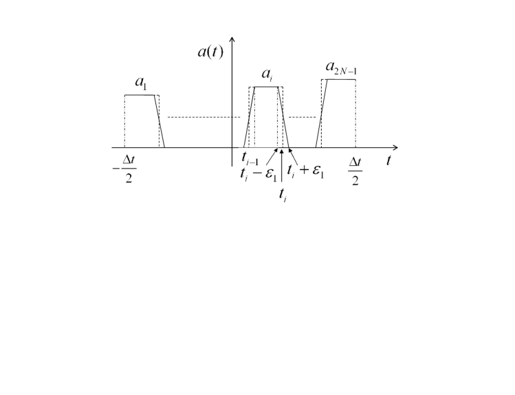
Figure 5: Piecewise constant accelerations having smooth change at the temporal boundaries.

We assume that $2\varepsilon_{1}>>\tau_{0},$ where $\tau_{0}$ (see Ref.moni ) is defined by

$$\tau_{0}=\frac{2}{3}\frac{q^{2}}{mc^{3}}.$$

Now,

$$\dot{\vec{a}}(\tau_{i})=\left\{\begin{array}[]{l}-\frac{{\vec{a}_{2i-1}}}{{2\varepsilon_{1}}},t_{2i-1}-\varepsilon_{1}\leq\tau_{i}\leq t_{2i-1}+\varepsilon_{1}(i=1,2,...,N-1){\rm{}}\\ \frac{{\vec{a}_{2i-1}}}{{2\varepsilon_{1}}},t_{2i-2}-\varepsilon_{1}\leq\tau_{i}\leq t_{2i-2}+\varepsilon_{1}(i=2,3,...,N)\\ \end{array}\right.$$

The quantity $\left\langle{\dot{\vec{a}}}\right\rangle$ now turns out:

$$\left\langle{\dot{\vec{a}}}\right\rangle = \frac{1}{{\Delta t}}\int\limits_{-\frac{{\Delta t}}{2}}^{\frac{{\Delta t}}{2}}{\sum\limits_{i=1}^{N}{\dot{\vec{a}}({\tau_{i}})}d\tau_{i}}$$ (27)

$$= \frac{{\vec{a}_{2N-1}-\vec{a}_{1}}}{{\Delta t}}$$ (28)

References

- (1) A.K.Singal, 2011, An ab initio derivation of the electromagnetic fields of a point charge in arbitrary motion, Am. J. Phys. 79, 1036 (2011).
- (2) J. J. Thomson, Electricity and Matter(Charles Scribners, New York, 1904), chap. 3.
- (3) J. D. Jackson, Classical Electrodynamics (New York: John Wiley & Sons, 2003).
- (4) Asrarul Haque, 2014, A simple derivation of Lorentz self-force, Eur. J. Phys. 35 (2014) 055006 (8pp).
- (5) Julian Schwinger, L. L. DeRaad, K.A. Milton and W. Tsai, Classical Electrodynamics(Perseus Press, New York,1998) , chap. 37.
- (6) David J. Griffiths, 1999, Introduction to Electrodynamics, 3rd ed., section 12.2 and 12.3.
- (7) E.J. Moniz and D. H. Sharp, Phys. Rev. D 15,2850 (1977), F. Rohrlich, Phys. Rev. E 77,046609 (2008).