Symmetry-protected topological order in magnetization plateau states of quantum spin chains

Abstract

A symmetry-protected topologically ordered phase is a short-range entangled state, for which some imposed symmetry prohibits the adiabatic deformation into a trivial state which lacks entanglement. In this paper we argue that magnetization plateau states of one-dimensional antiferromagnets which satisfy the conditions $S-m\in$ odd integer, where $S$ is the spin quantum number and $m$ the magnetization per site, can be identified as symmetry-protected topological states if an inversion symmetry about the link center is present. This assertion is reached by mapping the antiferromagnet into a nonlinear sigma model type effective field theory containing a novel Berry phase term (a total derivative term) with a coefficient proportional to the quantity $S-m$, and then analyzing the topological structure of the ground state wave functional which is inherited from the latter term. A boson-vortex duality transformation is employed to examine the topological stability of the ground state in the absence/presence of a perturbation violating link-center inversion symmetry. Our prediction based on field theories is verified by means of a numerical study of the entanglement spectra of actual spin chains, which we find to exhibit twofold degeneracies when the aforementioned condition is met. We complete this study with a rigorous analysis using matrix product states.

I Introduction

Classification of phases is an important and fundamental problem in statistical physics. In Ginzburg-Landau theories, different phases are distinguished by local order parameters. It has come to be realized in the past few decades, however, that there are phases which cannot be characterized by local order parameters but are nevertheless nontrivial. Dubbed topologically ordered phases, they have in recent years become an intensively studied subject in condensed matter physics Wen04 . There are largely two known types of topological orders. One is characterized by states with long-range entanglement that sustain anyonic excitations. The other arises in states with short-range entanglement and become robust as a phase when some specific symmetries are imposed; the imposed symmetry condition forbids perturbative terms, whose incorporation would otherwise smoothly deform the state into a direct product (i.e., topologically trivial) state. States characterized by the latter type of order are said to belong to a symmetry-protected topological (SPT) phase.

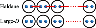
Figure 1: (Color online) Schematic pictures of $S=1$ Haldane (VBS) and large-$D$ phases. The links connecting spin-1/2’s (balls) represent singlet bonds.

A typical example of an SPT phase is the Haldane state Haldane83 ; Affleck87 of $S=1$ quantum magnets, which is conveniently characterized as a valence bond solid (VBS) [Fig. 1]. Haldane conjectured that Heisenberg antiferromagnets composed of integer spin have a nonzero excitation gap, while those with half-integer spin are gapless. Decades after this prediction was verified through many numerical calculations and experiments Nightingale86 ; White93 ; Polizzi98 ; Katsumata89 , recent studies motivated by the quest for new topological phases of matter have made it apparent that even within the gapped ground states for integer spin systems, there is a qualitative difference between the $S=$ odd and even cases. For example, in the $S=1$ case, it was shown that a phase transition must always intervene between the Haldane phase and a topologically trivial phase (a typical example of the latter being the large-$D$ phase [Fig. 1], which can be expressed in the $S^{z}$ basis as $|\ldots 0000\ldots\rangle$) provided one of the following three symmetries is imposed onto the system Pollmann10 : (i) the dihedral group of $\pi$ rotations about the $x,y,z$ axes, (ii) time-reversal, and (iii) link-center inversion. For $S=2$ chains, in contrast, it is possible to connect the Haldane and large-$D$ phases adiabatically Pollmann10 . Phases in one-dimensional gapped spin chains can thus be enriched by symmetry protection Chen11 and their classification using group cohomology has been put forth Chen12 . SPT phases in higher dimensions have also been proposed Levin12 ; Lu12 ; Senthil13 ; Vishwanath13 ; Ye13 .

Gapped phases are also observed in antiferromagnets under an externally applied magnetic field. These are the magnetization plateaus, i.e., the regions within the magnetization curve where the magnetization remains unchanged with increasing field strength. The Oshikawa-Yamanaka-Affleck (OYA) theory generalizes the celebrated Lieb-Schultz-Mattis theorem Lieb61 and summarizes the necessary condition for the appearance of a plateau in the form $r(S-m)\in\mathbb{Z}$, where $r$ is the number of sites in one unit cell and $S$ is the spin quantum number and $m$ the magnetization per site Oshikawa97 ; Totsuka97 . The stability of this gapped plateau phase has also be explained in terms of an effective field theory where Berry phase terms play a crucial role Tanaka09 . Strong analogies between the Haldane gap and magnetization plateau states have been noted early on Oshikawa97 , and a VBS picture similar to Fig. 1 can be employed to depict the latter (see, e.g., Fig. 7). In view of the current interest in physical realizations of SPT states, it would thus seem important to search for magnetization plateau states which can be characterized as an SPT phase. This is the principal purpose of the present work. We note that there are several previous studies on magnetization plateaus which have also been conducted in the light of topological phases (though the explicit connection with SPT phases was not addressed): for instance, the Chern number and nontrivial edge excitations associated with plateau state in periodically modulated chains was discussed in Ref. Hu14 , while the entanglement spectra of plateau states which occur in ferro-ferro-antiferromagnetic (FFAF) chains was investigated in Ref. Takayoshi14 .

An additional motivation comes from the correspondence Sachdev11 ; Tanaka09 between antiferromagnets subjected to a magnetic field and bosons with a tunable chemical potential (which can be casted into a Bose-Hubbard model Fisher89 ). SPT states which appear in the phase diagram of the Bose-Hubbard model have been proposed DallaTorre06 ; Batrouni13 , and new developments in cold-atom experiments enable one to directly measure string orders Endres11 which, in principle, detect the subtle topological orders which characterize such states. It is our hope that the present study will contribute some new insights to this closely related problem.

This paper is organized as follows. We begin by developing in Sec. II an effective field theory for magnetization plateau states. In particular, we elicit a spin Berry phase term which will be central to the discussion that follows in Sec. III. This term has a surface contribution which was not considered in the earlier field theoretical work described in Ref. Tanaka09 . We then go on to investigate, following the path integral formalism of Ref. Xu13 , the topological structure of the ground state wave functional of our spin system. Here we will see that the surface Berry phase term will contribute a phase factor to the wave functional through the presence of a temporal surface term, i.e., a temporal analog of the boundary Berry phase Ng94 which represents the fractional spins which appear at the end of open spin chains. We show that this factor will govern whether or not the ground state belongs to an SPT phase. Our finding is that a plateau state can be in an SPT phase if $S-m$ is an odd integer. We also make clear that this SPT phase is protected by the link-center inversion (parity) symmetry $Z_{2}^{\rm P}$ by demonstrating that the protection of this phase is broken with the presence of staggered magnetic field. In Sec. IV, we verify affirmatively this prediction by presenting numerical calculations for model spin systems giving rise to plateaus satisfying $S-m\in$ odd and $S-m\in$ even. This is carried out by examining the degeneracy of the entanglement spectrum, which provides a direct fingerprint of SPT order. Finally, in Sec. V we present a matrix product state (MPS) construction for the $m=1/2$ plateau in $S=3/2$ chains, which enables us to confirm in a rigorous manner that this state is indeed an SPT phase. Section VI is devoted to discussions and a summary. In the Appendix, the classification of SPT phases protected by ${\rm U(1)}\rtimes Z_{2}^{\rm P}$ is discussed using the MPS representation.

II Effective field theory of magnetization plateau phases: topological terms

A field-theoretical description of the magnetization plateau state which emphasizes the role played by Berry phases was formulated in Ref. Tanaka09 . In the following we refine this treatment in such a way that exposes the relation of this state to SPT phases. For simplicity, we hereon assume that a unit cell contains only one site, in which case the OYA condition reads $S-m\in\mathbb{Z}$. Following Ref. Tanaka09 , we shall start with the following Hamiltonian which describes an antiferromagnetic spin chain in an external magnetic field,

$${\cal H}=J\sum_{j}\boldsymbol{S}_{j}\cdot\boldsymbol{S}_{j+1}+D\sum_{j}(S_{j}^{z})^{2}-H\sum_{j}S_{j}^{z}.$$ (1)

We assume a canted spin configuration:

$$\boldsymbol{S}_{j}=S\boldsymbol{n}_{j}=\begin{pmatrix}\sqrt{S^{2}-m_{j}^{2}}\cos(kx)\\ \sqrt{S^{2}-m_{j}^{2}}\sin(kx)\\ m_{j}\end{pmatrix}\quad(x=ja),$$ (2)

where $a$ is a lattice constant and $k=\pi/a$. Spins are aligned in an antiparallel fashion within the $xy$ plane, while the $z$ component is uniform. As depicted in Fig. 2, we parametrize the corresponding unit vector $\boldsymbol{n}_{j}$ using spherical coordinates

$$\boldsymbol{n}_{j}(\tau)=\begin{pmatrix}(-1)^{j}\cos\phi_{j}(\tau)\sin\theta_{0}\\ (-1)^{j}\sin\phi_{j}(\tau)\sin\theta_{0}\\ \cos\theta_{0}\end{pmatrix}.$$

The magnetization is $m=S\cos\theta_{0}$. For the classical solution, $\cos\theta_{0}=H/(2S(D+2J))$. We follow the treatment of Ref. Tanaka09 in regard to the magnetization and hence $\theta_{0}$ for a given value of the magnetic field as fixed, taking into account the massive nature of the fluctuation of the latter quantity.

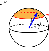
Figure 2: (Color online) Schematic pictures of the spin Berry phase for magnetization plateau states in spherical coordinates.

The effective action for (1) can be divided into the kinetic term ${\cal S}_{\rm kin}$ and the Berry phase contribution ${\cal S}_{\rm BP}^{\rm tot}$,

$${\cal S}={\cal S}_{\rm kin}+{\cal S}_{\rm BP}^{\rm tot},\quad{\cal S}_{\rm kin}=\int d\tau{\cal H}.$$ (3)

The continuum limit of the kinetic term is Tanaka09

$${\cal S}_{\rm kin}\;\to\;\int d\tau dx\frac{\zeta}{2}\Big{\{}\frac{1}{v^{2}}(\partial_{\tau}\phi)^{2}+(\partial_{x}\phi)^{2}\Big{\}},$$

where

$$\zeta= aJS^{2}\Big{(}1-\frac{H^{2}}{4S^{2}(D+2J)^{2}}\Big{)},$$

$$v= Ja\sqrt{\frac{4S^{2}(D+2J)^{2}-H^{2}}{2J(D+2J)}}.$$

The Berry phase part of the action (3) is the summation of the contribution from each site. For the sake of the following discussion, it proves convenient to introduce an auxiliary vector

$$\boldsymbol{N}_{j}(\tau)\equiv\begin{pmatrix}\cos\phi_{j}(\tau)\sin\theta_{0}\\ \sin\phi_{j}(\tau)\sin\theta_{0}\\ \cos\theta_{0}\end{pmatrix}.$$ (4)

We note that the spin Berry phase term for $\boldsymbol{n}(\tau)$ coincides with that for $\boldsymbol{N}_{j}(\tau)$. This follows since both spins precess in the same direction around the $z$ axis along the same constant latitude. The total Berry phase is ${\cal S}_{\rm BP}^{\rm tot}=\sum_{j}{\cal S}_{\rm BP}[\boldsymbol{N}_{j}(\tau)]$, where

$${\cal S}_{\rm BP}[\boldsymbol{N}_{j}(\tau)]= iS(1-\cos\theta_{0})\int d\tau\partial_{\tau}\phi_{j}$$

$$= i(S-m)\int d\tau\partial_{\tau}\phi_{j}.$$ (5)

Applying the identity

$${\cal S}_{\rm BP}[\boldsymbol{N}_{j}(\tau)]=2i(S-m)\int d\tau\partial_{\tau}\phi_{j}-{\cal S}_{\rm BP}[\boldsymbol{N}_{j}(\tau)]$$

only to terms associated with $j=$ even sites, we recast ${\cal S}^{\rm tot}_{\rm BP}$ as

$${\cal S}_{\rm BP}^{\rm tot}= \sum_{j{\rm:odd}}{\cal S}_{\rm BP}[\boldsymbol{N}_{j}(\tau)]$$

$$+\sum_{j{\rm:even}}\Big{[}2i(S-m)\int d\tau\partial_{\tau}\phi-{\cal S}_{\rm BP}[\boldsymbol{N}_{j}(\tau)]\Big{]}$$

$$= \sum_{j}(-1)^{j}{\cal S}_{\rm BP}[\boldsymbol{N}_{j}(\tau)]+\sum_{j{\rm:even}}2i(S-m)\int d\tau\partial_{\tau}\phi_{j}.$$ (6)

In the continuum limit, the second term of the last line of (6) reads

$$\sum_{j{\rm:even}}2i(S-m)\int d\tau\partial_{\tau}\phi_{j}\;\to\;i\int d\tau dx\frac{S-m}{a}\partial_{\tau}\phi.$$ (7)

This is the Berry phase term that was derived in Ref. Tanaka09 . There it was argued, by incorporating a a boson-vortex duality transformation, that for the case $S-m\notin\mathbb{Z}$, this term has a nontrivial effect and will generally lead to a gapless theory by prohibiting vortex condensation. Meanwhile, for $S-m\in\mathbb{Z}$, it was found that this term does not affect the low-energy physics, allowing for vortex proliferation and hence the formation of a gapped (i.e., the magnetization plateau) state. As we are focused on the latter situation, this term can be discarded.

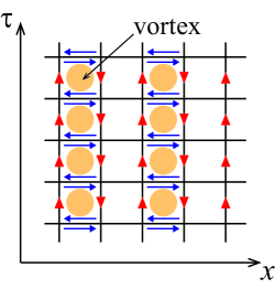
Figure 3: (Color online) Following Ref. Sachdev02 , we take a summation over spin Berry phases with an alternating sign (vertical arrows), which amounts to counting the vorticity in every other row. The horizontal arrows cancel due to the contributions from adjacent plaquettes.

We now turn to the first term of the last line of (6), which was previously not considered. By placing the system on a space-time grid, the summation over spin Berry phases with an alternating sign can conveniently be converted into a net space-time vorticity Sachdev02 as schematically shown in Fig. 3. We therefore have

$${\cal S}_{\rm BP}^{\rm tot}= \sum_{j}(-1)^{j}{\cal S}_{\rm BP}[\boldsymbol{N}_{j}(\tau)]$$

$$= i\sum_{j}(-1)^{j}(S-m)\int d\tau\partial_{\tau}\phi_{j}$$

$$= i2\pi(S-m)\sum_{\begin{subarray}{c}\rm odd\\ \rm column\end{subarray}}({\rm spacetime\;vorticity\;of}\;\phi).$$

Taking the continuum limit, we obtain

$${\cal S}_{\rm BP}^{\rm tot}\to i\frac{S-m}{2}\int d\tau dx(\partial_{\tau}\partial_{x}-\partial_{x}\partial_{\tau})\phi(\tau,x)$$

$$\equiv i\pi(S-m)Q_{\rm v},$$ (8)

where the factor 1/2 in the first line can be understood by observing that we are to add up the total vorticity in every other row, and $Q_{\rm v}$ is the net vorticity throughout the entire space-time.

In order to gain an understanding on the physics which is represented by the action (8), it is insightful to compare this topological term with that which appears in the effective theory of a planar antiferromagnetic chain (without an applied magnetic field). It is well known that the O(3) nonlinear $\sigma$ (NL$\sigma$) model with a topological $\theta$ term captures the low-energy property of an antiferromagnetic spin chain. One way to incorporate the planar nature of the order parameter into this action while preserving the global topological properties of the theory, is to employ the CP¹ representation Auerbach , which re-expresses the planar unit vector

$$\boldsymbol{N}_{\rm pl}(\tau,x)\equiv\begin{pmatrix}\cos\phi(\tau,x)\\ \sin\phi(\tau,x)\\ 0\end{pmatrix}$$

in terms of a spinor field $\boldsymbol{z}$ through the relation $N_{\rm pl}^{a}=\boldsymbol{z}^{\dagger}\sigma^{a}\boldsymbol{z}$ ($\sigma^{a}$: Pauli matrices). Choosing the gauge

$$\boldsymbol{z}\equiv\begin{pmatrix}1/\sqrt{2}\\ e^{i\phi(\tau,x)}/\sqrt{2}\end{pmatrix},$$

we find that the CP¹ gauge field is

$$a_{\mu}\equiv-i\boldsymbol{z}^{\dagger}\partial_{\mu}\boldsymbol{z}=\partial_{\mu}\phi/2\;(\mu=\tau,x).$$

Finally, plugging this into the CP¹ representation for the $\theta$ term Auerbach ,

$${\cal S}_{\theta}=i\frac{\theta}{2\pi}\int d\tau dx(\partial_{\tau}a_{x}-\partial_{x}a_{\tau}),$$

where the vacuum angle $\theta$ (not to be confused with the spherical coordinate) is $\theta=2\pi S$, we arrive at

$${\cal S}_{\theta}^{\rm pl}=i\pi SQ_{\rm v},$$ (9)

which is consistent with the lattice-based results of Ref. Sachdev02 . Also, as explained later in this section, it is possible to start from Eq. (9) to derive a dual vortex field theory which, when treated with due care, correctly discriminates the behavior of integer- and half-integer-$S$ systems in agreement with the Haldane conjecture. This fact lends credibility to the use of this particular expression in the continuum theory.

Comparing Eqs. (8) and (9), and noting in addition that the kinetic term of our action bears the form of an O(3) NL$\sigma$ model in the XY limit, we find that the two effective theories are identical in form. In particular, Eq. (8) corresponds exactly to the $\theta$ term ${\cal S}_{\theta}^{\rm pl}$ with an effective vacuum angle of

$$\theta_{\rm eff}=2\pi(S-m).$$

This coincidence is quite natural when we recall the VBS-construction of a magnetization plateau state, such as depicted in Fig. 7. At each site, the dynamics of the polarized portion of the spin moment (of magnitude $m$) is pinned down by the magnetic field, while the subsystem consisting of the remaining “active” moment of magnitude $S-m$ form a VBS-like state. The low-energy physics of this state is therefore essentially that of (the planar limit of) a Haldane gap state of a spin $S-m$ antiferromagnet (recall that we are confining our attention to the case where $S-m\in\mathbb{Z}$). It is also worthwhile to note that the Berry phase action, Eq. (8), is a total derivative term, which will have important consequences in the following section.

In the remainder of this section, we discuss how the application of a duality transformation on the effective action obtained above:

$${\cal S}= {\cal S}_{\rm kin}+{\cal S}_{\rm BP}^{\rm tot},$$

$${\cal S}_{\rm kin}= \int d\tau dx\frac{\zeta}{2}\Big{\{}\frac{1}{v^{2}}(\partial_{\tau}\phi)^{2}+(\partial_{x}\phi)^{2}\Big{\}},$$ (10)

$${\cal S}_{\rm BP}^{\rm tot}= i(S-m)\int d\tau dx(\partial_{\tau}a_{x}-\partial_{x}a_{\tau}),$$

will enable us to seek additional insight from the viewpoint of vortex condensates. Since (i) the action (10) is basically a quantum XY model, and (ii) vortex proliferation is allowed in the magnetization plateau phase, it is not difficult to guess that the dual vortex-field theory will come out as some variant of the quantum sine-Gordon action, a fact which will be verified shortly. Though the technicalities involved in carrying out the “dual-izing” procedure were described in some details in Ref. Tanaka09 , we briefly sketch the main steps as there are differences stemming from use of a different topological term. For the sake of simplicity, the mapping will be performed in the continuum limit. The corresponding procedures can, however, be carried out on the lattice as well, which can easily be seen to lead to identical results.

We start then, with a slight rewriting of the effective Lagrangian density:

$${\cal L}=\frac{1}{2g}(\partial_{\mu}\phi)^{2}+i\pi(S-m)\rho_{\rm v},$$

where $\rho_{\rm v}\equiv(\partial_{\tau}\partial_{x}-\partial_{x}\partial_{\tau})\phi/(2\pi)$ is the density of spacetime vortices. Here we have set $v=1$ and $g=1/\zeta$ for notational simplicity. A Hubbard-Stratonovich transformation recasts the kinetic term as $(\partial_{\mu}\phi)^{2}/(2g)\to(g/2)J_{\mu}^{2}+iJ_{\mu}\partial_{\mu}\phi$. After decomposing $\phi$ into a vortex-free portion $\phi_{\rm r}$ and a portion with vorticity $\phi_{\rm v}$, i.e., $(\partial_{\tau}\partial_{x}-\partial_{x}\partial_{\tau})\phi_{\rm r}=0$ and $(\partial_{\tau}\partial_{x}-\partial_{x}\partial_{\tau})\phi_{\rm v}\neq 0$, the integration over $\phi_{\rm r}$ yields a delta function contribution $\propto\delta(\partial_{\mu}J_{\mu})$. The constraint $\partial_{\mu}J_{\mu}=0$ is formally solved by introducing a new vortex-free scalar field $\varphi$ and putting $J_{\mu}\equiv\epsilon_{\mu\nu}\partial_{\nu}\varphi/(2\pi)$, which leads to

$${\cal L}=\frac{g}{8\pi^{2}}(\partial_{\mu}\varphi)^{2}+i\big{[}\pi(S-m)-\varphi\big{]}\rho_{\rm v}.$$

Integrating out the dual field $\varphi$, we obtain

$${\cal L}_{\rm dual}=\frac{2\pi^{2}}{g}\rho_{\rm v}\frac{1}{-\partial^{2}}\rho_{\rm v}+i\pi(S-m)\rho_{\rm v}.$$

This is the dual action for vortices written at the first quantization level, describing the intervortex logarithmic interaction (first term) and the vortex Berry phase (second term).

Alternatively one can proceed to derive a vortex field theory, i.e., a dual theory at the second quantization level. For this purpose, we submit the system to a standard fugacity expansion and restrict the vorticity to $\pm 1$. Denoting the fugacity as $z=e^{-\mu}$, where $\mu$ is the creation energy of a vortex, the grand canonical partition function of the vortex gas becomes

$$Z= \int{\cal D}\varphi e^{-\int d^{2}\boldsymbol{x}(g/(8\pi^{2}))(\partial_{\mu}\varphi)^{2}}\sum_{N_{+}=0}^{\infty}\sum_{N_{-}=0}^{\infty}\frac{(ze^{i\pi(S-m)})^{N_{+}}}{N_{+}!}\frac{(ze^{-i\pi(S-m)})^{N_{-}}}{N_{-}!}\Big{(}\int d^{2}\boldsymbol{r}_{i_{+}}e^{-i\varphi(\boldsymbol{r}_{i_{+}})}\Big{)}^{N_{+}}\Big{(}\int d^{2}\boldsymbol{r}_{i_{-}}e^{i\varphi(\boldsymbol{r}_{i_{-}})}\Big{)}^{N_{-}}$$

$$= \int{\cal D}\varphi\exp\Big{[}-\int d^{2}\boldsymbol{x}\Big{\{}\frac{g}{8\pi^{2}}(\partial_{\mu}\varphi)^{2}+2z\cos\big{[}\pi(S-m)-\varphi\big{]}\Big{\}}\Big{]}.$$

Taking into account the condition $S-m\in\mathbb{Z}$, the final form of the vortex field theory reads

$${\cal L}_{\rm dual}=\frac{g}{8\pi^{2}}(\partial_{\mu}\varphi)^{2}+2z\cos\big{[}\pi(S-m)\big{]}\cos\varphi.$$ (11)

Having started with a new Berry phase term which only applies to the plateau state, our vortex field theory differs from the one found in Ref. Tanaka09 . The Berry phase for each space-time vortex event is reflected in the coefficient $\cos\big{[}\pi(S-m)\big{]}$ of the cosine term. This cosine term has scaling dimension $\pi/g$, and becomes relevant when $g>\pi/2$, in which regime the field $\varphi$ ($\phi$) is ordered (disordered), due to vortex proliferation. Because of the sign dependence of the cosine term in (11) on the parity of $S-m$, a different value of $\varphi$ is favored depending on whether $S-m$ is odd or even. While this suggests that the two cases describe two distinct phases Fuji14 , we shall postpone their characterization as SPT or trivial phases until Sec. III, where a fuller picture will emerge by relating the behavior of the dual theory (11) to the topological structure of the ground state wave functional.

One thing that follows immediately from the above action is that a phase-soliton of height $\pi$ must exists at a junction of $S-m=$ even and odd systems. We can surmise that this soliton carries a spin-1/2, which would correspond to a boundary spin. This is conveniently seen by refermionizing the bosonic field $\varphi$ to right and left moving fermions $R,L$. For simplicity, let us suppose that the Luttinger liquid parameter $g$ is tuned such that the first term in (11) corresponds to the free Dirac fermion (i.e., $g=\pi$). The Lagrangian (11) then is equivalent to the following massive Dirac fermion

$${\cal L}_{\rm fer}=\bar{\psi}\gamma^{\mu}\partial_{\mu}\psi+M\bar{\psi}\psi,$$

where $\psi^{\rm T}=(R,L)$, $\gamma_{0}=\sigma_{1}$, $\gamma_{1}=-\sigma_{2}$, $\gamma_{5}=\sigma_{3}=i\gamma_{0}\gamma_{1}$, $\bar{\psi}=\psi^{\dagger}\gamma_{0}$, and $M=16\pi z\cos\big{(}\pi(S-m)\big{)}$ ($\sigma_{1,2,3}$ are Pauli matrices). Through the relations:

$$i(\partial_{\tau}-i\partial_{x})\varphi/(4\pi)\leftrightarrow :R^{\dagger}R:$$

$$-i(\partial_{\tau}+i\partial_{x})\varphi/(4\pi)\leftrightarrow :L^{\dagger}L:,$$

the charge density of fermions is represented as

$$\rho\equiv:R^{\dagger}R+L^{\dagger}L:=\partial_{x}\varphi/(2\pi).$$

For $S-m=$ even (odd) systems, the fermion mass $M$ is positive (negative) and $\varphi$ is pinned at $\pi$ (0). If $S-m=$ even (odd) in $x>0$ ($x\leq 0$), the fermion charge is

$$\int_{-\infty}^{\infty}dx\rho=\int_{-\infty}^{\infty}dx\frac{\partial_{x}\varphi}{2\pi}=\frac{1}{2}.$$

This implies that a soliton with fractionalized charge exists at the boundary between $S-m=$ odd and even systems. This soliton corresponds to the boundary spin-1/2 stated above. The action (11) also tells us that, even for the same sign of $z$, we may have different types of plateaus depending on the parity of $S-m$. We will see examples of this in Sec. IV.

Finally we mention that a quantum XY model with the Berry phase term of Eq. (9), which describes planar antiferromagnetic chains in the absence of external fields, can be submitted to the same duality procedures of the proceeding paragraphs. The final vortex field theory is identical in form to the sine-Gordon action (11), but with $S-m$ replaced by $S$. (Here a slight subtlety must be accounted for to reach this form. Namely, we need to assume for this purpose that the system is an easy-plane antiferromagnet, and the spin would prefer to escape into the out-of-plane direction at the vortex core, which would be less costly than creating a singular core. It is important to notice at this point that for a given winding sense of a vortex configuration, there are two possible (up and down) directions in which the spin at the core can point. Taking all four topological (meron) configurations into account, we arrive at the dual theory mentioned above Affleck89 .) If $S$ is a half-odd integer, the coefficient $\cos(\pi S)$ vanishes identically, yielding a massless theory, while the cosine term can generate a mass gap for integer $S$. The consistency of this result with the Haldane conjecture provides a useful check on the validity of the type of field theory that we have discussed in this section.

III Temporal surface terms and the SPT order in magnetization plateau states

Having arrived at our effective action (10), we are in a position to discuss, along the lines of Ref. Xu13 , the possible emergence of SPT order in a magnetization plateau state. The basic strategy is to express the ground state wave functional using a Feynman path integral representation, and thereby isolate the phase factor which comes from a temporal surface contribution generated by the Berry phase term. (Imposing a periodic boundary condition along the spatial direction, as we will do below, implies that the action does not contain the more familiar spatial surface contributions.) One finds that this temporal surface term encodes into the wave functional the information necessary to discriminate between states with and without the SPT order.

Here we will take the strong coupling limit $\zeta\to 0$, and only consider the topological part of the action, although this is not an absolute necessity and will not effect the conclusions. Focusing primarily on bulk properties, we will employ spatial periodic boundary conditions. The state vector for the ground state can be expanded with respect to the basis $|\boldsymbol{N}_{\rm pl}(x)\rangle$, which we use as a shorthand notation for the spin coherent state corresponding to the snapshot configuration $\{\boldsymbol{N}_{\rm pl}(x)\}$,

$$|\Psi_{\rm GS}\rangle=\sum_{\boldsymbol{N}_{\rm pl}(x)}\Psi[\boldsymbol{N}_{\rm pl}(x)]|\boldsymbol{N}_{\rm pl}(x)\rangle.$$

Each coefficient (wave functional) $\Psi[\boldsymbol{N}_{\rm pl}(x)]$ stands for the probability amplitude that the configuration $\{\boldsymbol{N}_{\rm pl}(x)\}$ occurs in the ground state, and can formally be expressed in path integral language as an evolution in imaginary time starting from some initial configuration:

$$\Psi[\boldsymbol{N}_{\rm pl}(x)]\propto\int_{\boldsymbol{N}_{\rm pl,i}}^{\boldsymbol{N}_{\rm pl,f}=\boldsymbol{N}_{\rm pl}(x)}{\cal D}\boldsymbol{N}^{\prime}_{\rm pl}(\tau,x)e^{-{\cal S}[\boldsymbol{N}^{\prime}_{\rm pl}(\tau,x)]}.$$ (12)

Here, $\boldsymbol{N}_{\rm pl,i(f)}\equiv\boldsymbol{N}^{\prime}_{\rm pl}(\tau_{\rm i(f)},x)$ represents spin configurations at initial (final) imaginary time $\tau_{\rm i(f)}$. Substituting the expression for the Berry phase term in (10) into (12), and taking into account the spatial periodic boundary condition yields

$$\Psi[ \boldsymbol{N}_{\rm pl}(x)]$$

$$\propto\int_{\boldsymbol{N}_{\rm pl,i}}^{\boldsymbol{N}_{\rm pl}(x)}{\cal D}\boldsymbol{N}^{\prime}_{\rm pl}(\tau,x)e^{-i(S-m)\int dx[a_{x}(\tau_{\rm f})-a_{x}(\tau_{\rm i})]}.$$

Localized at the two ends of the interval on which the imaginary-time integration is performed, the exponent in the right-hand side of the above equation may be viewed as the action contributed by temporal surface terms, as already mentioned. Since $a_{x}(\tau_{\rm i})$ is fixed by the initial condition and can be placed outside the path integral (a Feynman sum over initial configurations is to be performed afterwards), we need only concern ourselves with the term involving $a_{x}(\tau_{\rm f})$, and we are left with

$$\Psi[\boldsymbol{N}_{\rm pl}(x)]\propto e^{-i(S-m)\pi W},$$ (13)

where $W\equiv(1/2\pi)\int dx\partial_{x}\phi\in\mathbb{Z}$ is the winding number which records the number of times the planar vector $\boldsymbol{N}_{\rm pl}(x)$ wraps around its circular target space as we follow its orientation along the spatial extent of the system.

For $S-m={\rm even}$, $e^{i(S-m)\pi W}\equiv 1$ and the wave functional (13) reduces to that in the absence of the topological term. The case where $S-m=$ odd, meanwhile, yields the nontrivial factor $(-1)^{W}$. This suggests that the ground states break up into two sectors, i.e., that odd-($S-m$) plateaus are SPT states that are topologically distinct from the even-($S-m$) states, which we expect to be topologically trivial. The construction of SPT states by modifying signs of the trivial wave functional is close in spirit to the construction of the Ising-like SPT in two dimensions from a trivial paramagnetic state Levin12 . To verify this assertion it remains to identify, as we will address in a moment, the symmetry (or symmetries) which can protect this distinction (i.e., prevent the addition of perturbations that will cause the wave functional to adiabatically interpolate between the above two sectors).

We mention in passing that we have restricted our attention to the case where the unit cell consists of one site. The extension of our treatment to a system with $r$ sites per cell is straightforward. There the parity of

$$r(S-m)\in\mathbb{Z}$$ (14)

(where $m$ still stands for the magnetization per site) will replace the role of $S-m$ of the present argument.

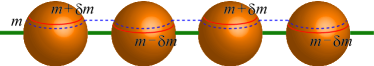
Figure 4: (Color online) Application of a staggered magnetic field along the $z$ axis alters the local magnetization from $S-m$ to $S-m+(-)^{j}\delta m$, which clearly results in the breakdown of the structure (13). This perturbation can be prohibited by imposing a link-center inversion symmetry on the system.

Let us now consider the effect of applying a staggered magnetic field along the $z$ axis [Fig. 4]. Repeating the derivation of the total Berry phase for this case, it is clear that this is the generic perturbation that directly affects the first (sign-alternating) term of (6), leading to the modification $S-m\rightarrow S-m-\delta m$, while leaving unchanged the second (uniform) term. The latter contribution can therefore be discarded as before, and we are left with

$${\cal S}_{\rm BP}^{\rm tot}=i(S-m-\delta m)\int d\tau dx(\partial_{\tau}a_{x}-\partial_{x}a_{\tau}).$$

Accordingly, the wave functional formerly expressed by (13) now takes on the form

$$\Psi[\boldsymbol{N}_{\rm pl}(x)]\propto e^{-i(S-m-\delta m)\pi W}.$$

By varying $\delta m$, it is now possible to continuously interpolate between the two aforementioned dependencies of the wave functional on the winding number $W$. Additional information comes from revisiting the derivation of the vortex field theory (11); upon applying the staggered magnetic field, the action modifies to

$${\cal L}_{\rm dual}=\frac{g}{2}(\partial_{\mu}\varphi)^{2}+2z\cos\big{[}\pi(S-m-\delta m)-\varphi\big{]}.$$

It is clear from this action that the optimal value of the field $\varphi$ will change continuously as $\delta m$ is varied, without ever closing the energy gap. We therefore find that the application of a staggered magnetic field ruins the topological distinction between the even- and odd-($S-m$) cases. Since this perturbation can be prohibited by requiring that the system respect inversion symmetry with respect to the center of a link, our observations strongly suggest that the odd-($S-m$) plateaus are SPT states protected by link-center inversion symmetry and are distinct from the even-($S-m$) plateaus, which are topologically trivial. We will arrive at the same conclusion both through a numerical study in Sec. IV, and by analyzing an MPS representation for magnetization plateaus in Sec. V.

IV Numerical calculations

In this section, we numerically provide an independent confirmation of the prediction by field theories that the parity of $S-m$ determines whether the system is in SPT phase or not. A simple way to distinguish SPT and trivial phases is to investigate the degeneracy of the entanglement spectrum Pollmann10 . A numerical means suited for this purpose is the infinite time-evolving block decimation (iTEBD) Vidal07 . This method utilizes the ability of MPS to approximate gapped states and enables one to simulate infinite-size systems by assuming a certain sort of spatial periodicity in the ground state. Through the imaginary-time evolution, the state approaches the ground state optimally approximated within the MPS representation with a fixed matrix dimension $\chi$. In general, the true ground state is better approximated with larger $\chi$.

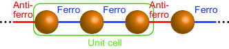
Figure 5: (Color online) An illustration of an FFAF chain. Each circle represents a spin-$S$ object. Two successive ferromagnetic couplings and one antiferromagnetic coupling residing on the nearest neighbor links are repeated as depicted.

An ideal quantum spin model for studying SPT phases in plateaus would be a Heisenberg model with single-ion anisotropy $D$ [Eq. (1)]. In fact, the existence of two different kinds of $m=1/2$ plateaus has been pointed out in this model with $S=3/2$ Kitazawa00 . It has been also argued there that the one appearing for small $D$ (i.e., $0.387\leq D/J\leq 0.943$) is characterized by the VBS-like state (where magnetization appears in the background of a VBS-like state) shown in Fig. 7(a). In addition, when $D$ further increases, a second-order Gaussian transition occurs and the system enters another plateau phase reminiscent of the large-$D$ phase, in which the unmagnetized background spin moments are quenched [Fig. 7(b)], and the short-range entanglement is absent.

It is easy to understand this fact in terms of our effective action (11). Observing that the sign of the coefficient $z\cos\big{[}\pi(S-m)\big{]}$ of the cosine term in (11) determines whether the system in question is topological or not, one immediately sees that the transition between the VBS-like and large-$D$ plateaus studied in Ref. Kitazawa00 should be characterized by $z=0$. This explains why the phase transition is of the Gaussian type. We note that this mechanism is essentially the same as that for the transition between the Haldane and large-$D$ phases in $S=1$ chains Schulz86 ; Chen03 . Unfortunately, this plateau appears only in a tiny window of the applied magnetic field $H$ and it is difficult to approach this state by iTEBD simulations with fixed $H$.

In order to circumvent the technical difficulties mentioned above, we study the following FFAF Heisenberg chain Hida94 [see Fig. 5]:

$${\cal H}_{\text{FFAF}}= \sum_{j=1}^{L}(-J_{\text{F}}\boldsymbol{S}_{3j-2}\cdot\boldsymbol{S}_{3j-1}-J_{\rm F}\boldsymbol{S}_{3j-1}\cdot\boldsymbol{S}_{3j}$$

$$\qquad+J_{\rm AF}\boldsymbol{S}_{3j}\cdot\boldsymbol{S}_{3j+1})-HS_{\rm tot}^{z},$$

where $L$ is the number of unit cells and $S_{\rm tot}^{z}\equiv\sum_{j=1}^{3L}S_{j}^{z}$. Coupling constants $J_{\rm F}$ and $J_{\rm AF}$ are both positive. Each unit cell consists of three spins which are coupled through ferromagnetic bonds [Fig. 5]. Due to the Hund rule coupling $-J_{\text{F}}$, we regard this unit cell as one spin-$3S$. Magnetization $m$ corresponds to $\langle S_{\rm tot}^{z}\rangle/L$. Thus, the situation is the same as considering plateaus with magnetization $\langle S_{\rm tot}^{z}\rangle/L$ in spin-$3S$ chains. We can give an equivalent description by substituting $r=3$ and $m=\langle S_{\rm tot}^{z}\rangle/(3L)$ into (14).

In particular, we performed calculations for $S=1/2$ and $S=1$ FFAF chains. We set the couplings at $J_{\rm F}=J_{\rm AF}=J$ for $S=1/2$ and $J_{\rm F}=J$, $J_{\rm AF}=2J$ for $S=1$. The magnetization curves of the $S=1/2$ and $S=1$ are shown in Figs. 6(a) and 6(b). We employed the iTEBD method with MPS dimensions of $\chi=150$ and 100 for $S=1/2$ and $S=1$, respectively. Magnetization plateaus appear at $\langle S_{\rm tot}^{z}\rangle/L=1/2$ for $S=1/2$ and at $\langle S_{\rm tot}^{z}\rangle/L=1,2$ for $S=1$ satisfying the OYA condition $3S-\langle S_{\rm tot}^{z}\rangle/L\in\mathbb{Z}$.

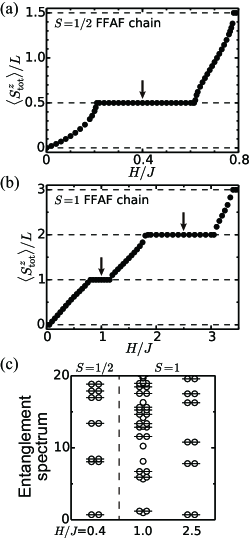
Figure 6: Magnetization curves of (a) $S=1/2$ and (b) $S=1$ FFAF chains. (c) Entanglement spectra obtained by the bipartition at an antiferromagnetic bond under $H/J=0.4$ for $S=1/2$, $H/J=1.0$ and 2.5 for $S=1$ (shown by arrows in panels (a), (b)). Calculations are performed using iTEBD.

In order to check if the above plateaus are topologically nontrivial, we investigate the entanglement spectrum Li08 which is known to give the fingerprints of topological phases. The entanglement spectrum of a quantum state $|\Psi\rangle$ is defined through the bipartition of the system into regions A and B. The state $|\Psi\rangle$ can be Schmidt-decomposed as a superposition of direct products $|\Psi\rangle=\sum_{\alpha}\lambda_{\alpha}|\Psi_{\rm A}\rangle_{\alpha}\otimes|\Psi_{\rm B}\rangle_{\alpha}$ using the orthonormal basis sets $\{|\Psi_{\text{A}}\rangle_{\alpha}\}$ and $\{|\Psi_{\text{B}}\rangle_{\alpha}\}$ of the subsystems. The entanglement spectrum is defined by the logarithm $\{-\ln(\lambda_{\alpha}^{2})\}$ $(\alpha=1,\ldots,\chi)$ of the Schmidt eigenvalues $\lambda_{\alpha}$ normalized as $\sum_{\alpha}\lambda_{\alpha}^{2}=1$. As will be discussed in Sec. V, if our system is in the SPT phase, the entanglement spectrum is twofold degenerate, in other words, all the values $\lambda_{\alpha}$ should appear in pairs. We emphasize that the bipartition of the system should be made at an antiferromagnetic bond since ferromagnetically coupled three spins are considered as one site. In Fig. 6(c), we present the entanglement spectra obtained for the plateau states at magnetic fields $H/J=0.4$ for $S=1/2$ and $H/J=1.0$ and 2.5 for $S=1$ [shown by arrows in Figs. 6(a) and 6(b)]. We can clearly see that entanglement spectra at $H/J=0.4$ ($\langle S_{\rm tot}^{z}\rangle/L=1/2$) for $S=1/2$ and at $H/J=2.5$ ($\langle S_{\rm tot}^{z}\rangle/L=2$) for $S=1$ exhibit twofold degeneracy while the one at $H/J=1.0$ ($\langle S_{\rm tot}^{z}\rangle/L=1$) for $S=1$ does not. These results imply that the system is in the SPT (trivial) phase for $3S-\langle S_{\rm tot}^{z}\rangle/L=$ odd (even), thus confirming the prediction from quantum field theories discussed in Sec. III.

In closing this section, we briefly remark on the connection between the findings of this section with the field theoretical study of the earlier sections. In Sec. III, we saw that the global structure of the ground state wave functional is determined by a temporal surface contribution coming from the topological term of the effective action. We can formally express the reduced density matrix $\rho_{\rm A}={\rm Tr}_{\rm B}|\Psi\rangle\langle\Psi|$ (where $|\Psi\rangle$ is the ground state and the trace operation is to be restricted to the region B), an object from which the entanglement spectrum can directly be extracted, along the same lines by incorporating a path integral representation Nishioka09 . Once again the topological term will give rise to a surface contribution, this time along a segment of the imaginary time axis bounded by the spatial edge of region A. While we expect that this will play an essential role in determining the entanglement spectrum, we leave the details for future work.

V MPS representation of plateau phases

In this section, we present a simple model ground state (MPS) that exhibits the SPT properties at finite magnetic fields and show that the degenerate structure found above in the entanglement spectrum is indeed closely tied to the underlying topological properties. We consider the $m=1/2$ plateau in a $S=3/2$ chain for example. On top of the trivial product state

$$\bigotimes_{j}|S_{j}^{z}=1/2\rangle\;,$$

we can think of an entangled state described by the VBS picture, schematically shown in Fig. 7. Using the auxiliary (Schwinger) bosons, this state is represented as

$$|\Psi\rangle=\prod_{j}a_{j}^{\dagger}(a_{j}^{\dagger}b_{j+1}^{\dagger}-b_{j}^{\dagger}a_{j+1}^{\dagger})\bigotimes_{j}|0\rangle_{j},$$ (15)

where $a_{j}^{\dagger}$ and $b_{j}^{\dagger}$ are the bosonic creation operators of spin-1/2 up and down on the $j$th site, respectively. Note that there are exactly three bosons at each site which guarantee a local spin-3/2 at each site. This is the exact ground state of the following $S=3/2$ Hamiltonian footnote1 :

$${\cal H}_{\rm VBS}=\sum_{j}\Big{\{}\boldsymbol{S}_{j}\cdot\boldsymbol{S}_{j+1}+ \frac{116}{243}(\boldsymbol{S}_{j}\cdot\boldsymbol{S}_{j+1})^{2}$$

$$+ \frac{16}{243}(\boldsymbol{S}_{j}\cdot\boldsymbol{S}_{j+1})^{3}\Big{\}}$$ (16)

with local magnetization 1/2.

The MPS representation of the above state is given by

$$|\Psi\rangle=C\sum_{S_{j}^{z}=-3/2}^{3/2}\cdots A[S_{j-1}^{z}]A[S_{j}^{z}]A[S_{j+1}^{z}]\cdots\bigotimes_{j}|S_{j}^{z}\rangle,$$ (17)

where

$$A[3/2]=\begin{pmatrix}0&0\\ -\sqrt{6}&0\end{pmatrix}, A[1/2]=\begin{pmatrix}\sqrt{2}&0\\ 0&-\sqrt{2}\end{pmatrix},$$

$$A[-1/2]=\begin{pmatrix}0&\sqrt{2}\\ 0&0\end{pmatrix}, A[-3/2]=\begin{pmatrix}0&0\\ 0&0\end{pmatrix}$$

and $C$ is a normalization constant. The transfer matrix of the MPS (17) is readily obtained as

$$T_{(\alpha_{1},\alpha_{2}),(\beta_{1},\beta_{2})}\equiv \sum_{S_{j}^{z}=-3/2}^{3/2}A_{\alpha_{1},\beta_{1}}^{*}[S_{j}^{z}]A_{\alpha_{2},\beta_{2}}[S_{j}^{z}]$$

$$= \begin{pmatrix}2&0&0&2\\ 0&-2&0&0\\ 0&0&-2&0\\ 6&0&0&2\\ \end{pmatrix}.$$

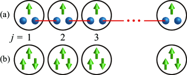
Figure 7: (Color online) (a) The VBS picture of a model plateau state (15) at $m=1/2$ in a $S=3/2$ spin chain. (b) Large-$D$ plateau.

An MPS representation is said to assume the canonical form Vidal03 ; PerezGarcia07 when its transfer matrix satisfies the condition

$$\begin{split}&\sum_{\alpha_{1},\alpha_{2}}\delta_{\alpha_{1},\alpha_{2}}T_{(\alpha_{1},\alpha_{2}),(\beta_{1},\beta_{2})}=\delta_{\beta_{1},\beta_{2}}\\ &\sum_{\beta_{1},\beta_{2}}T_{(\alpha_{1},\alpha_{2}),(\beta_{1},\beta_{2})}\delta_{\beta_{1},\beta_{2}}=\delta_{\alpha_{1},\alpha_{2}}\;.\end{split}$$ (18)

In order to discuss the SPT phase, it is convenient to work in the canonical form of the MPS. Since the MPS representation (17) does not satisfy (18), we first render it canonical using a gauge transformation $A\to M^{-1}AM$ ($M$ is some matrix). It is obvious that this transformation does not change the MPS. Taking

$$M=\begin{pmatrix}3^{-1/4}&0\\ 0&1\end{pmatrix},$$

we obtain the following canonical form of the MPS:

$$|\Psi\rangle=\sum_{S_{j}^{z}=-3/2}^{3/2}\cdots\Lambda\Gamma[S_{j-1}^{z}]\Lambda\Gamma[S_{j}^{z}]\Lambda\Gamma[S_{j+1}^{z}]\Lambda\cdots\bigotimes_{j}|S_{j}^{z}\rangle,$$ (19)

where the matrices are given by

$$\Gamma[3/2]=(1+\sqrt{3})^{-1/2}\begin{pmatrix}0&0\\ -\sqrt{2}\,3^{1/4}&0\end{pmatrix},$$

$$\Gamma[1/2]=(1+\sqrt{3})^{-1/2}\begin{pmatrix}\sqrt{2}&0\\ 0&-\sqrt{2}\end{pmatrix},$$

$$\Gamma[-1/2]=(1+\sqrt{3})^{-1/2}\begin{pmatrix}0&\sqrt{2}\,3^{1/4}\\ 0&0\end{pmatrix},$$

$$\Gamma[-3/2]=\begin{pmatrix}0&0\\ 0&0\end{pmatrix},$$

$$\Lambda=\begin{pmatrix}1/\sqrt{2}&0\\ 0&1/\sqrt{2}\end{pmatrix}.$$ (20)

The new MPS is related to the original one through the following similarity transformation:

$$M^{-1}A[S_{j}^{z}]M=(2+2\sqrt{3})^{1/2}\Lambda\Gamma[S_{j}^{z}].$$

We can check the condition (18) for the transfer matrix of the MPS (19)

$$T_{(\alpha_{1},\alpha_{2}),(\beta_{1},\beta_{2})}^{\rm can}\equiv \sum_{S_{j}^{z}=-3/2}^{3/2}(\Lambda\Gamma)_{\alpha_{1},\beta_{1}}^{*}[S_{j}^{z}](\Lambda\Gamma)_{\alpha_{2},\beta_{2}}[S_{j}^{z}]$$

$$= \sum_{S_{j}^{z}=-3/2}^{3/2}(\Gamma\Lambda)_{\alpha_{1},\beta_{1}}^{*}[S_{j}^{z}](\Gamma\Lambda)_{\alpha_{2},\beta_{2}}[S_{j}^{z}]$$

$$= \frac{1}{1+\sqrt{3}}\begin{pmatrix}1&0&0&\sqrt{3}\\ 0&-1&0&0\\ 0&0&-1&0\\ \sqrt{3}&0&0&1\\ \end{pmatrix},$$

and confirm that the MPS (19) is indeed in a canonical form.

Now let us discuss the protecting symmetry. In contrast to the $S=1$ Haldane phase, time-reversal and $Z_{2}\times Z_{2}$ symmetries are explicitly broken due to the presence of an external magnetic field. Nevertheless, the system still retains inversion symmetry with respect to the center of a link (link parity) and, as is already suggested from the field-theory argument in Sec.III, this symmetry will do the job. According to the discussion in Refs. Pollmann10 ; PerezGarcia08 , a projective representation $U_{\cal P}$ ($\chi\times\chi$ unitary matrix) of link-parity $\mathcal{P}$ satisfies

$$\Gamma=e^{i\theta_{\cal P}}U_{\cal P}^{\dagger}\Gamma^{\rm T}U_{\cal P}.$$ (21)

Using (21) twice, we see that the fundamental property $\mathcal{P}^{2}=1$ of the link-center inversion implies

$$\Gamma=e^{2i\theta_{\cal P}}(U_{\cal P}^{*}U_{\cal P})^{\dagger}\Gamma(U_{\cal P}^{*}U_{\cal P})$$

$$\Leftrightarrow (U_{\cal P}^{*}U_{\cal P})\Gamma=e^{2i\theta_{\cal P}}\Gamma(U_{\cal P}^{*}U_{\cal P}).$$

Multiplying $(\Gamma\Lambda)^{*}\Lambda$ from the left to this relation and taking the trace over the suffix $S^{z}$ in $\Gamma$, we obtain

$$(U_{\cal P}^{*}U_{\cal P})_{(\alpha_{1},\alpha_{2})}T_{(\alpha_{1},\alpha_{2}),(\beta_{1},\beta_{2})}^{\rm can}=e^{2i\theta_{\cal P}}(U_{\cal P}^{*}U_{\cal P})_{(\beta_{1},\beta_{2})}.$$

Here, note that $[U_{\cal P},\Lambda]=0$. Thus, $(U_{\cal P}^{*}U_{\cal P})$ is the left eigenvector of the transfer matrix $T^{\rm can}$. If we assume that unity is the unique largest eigenvalue of $T^{\rm can}$, then $e^{2i\theta_{\cal P}}=1$ and $U_{\cal P}^{*}U_{\cal P}=e^{i\phi_{\cal P}}E$ ($E$ is unit matrix). Using $U_{\cal P}=e^{i\phi_{\cal P}}U_{\cal P}^{\rm T}$ twice, $e^{2i\phi_{\cal P}}=1$. Thus, the phase $\phi_{\cal P}$ is quantized to 0 and $\pi$, which characterizes the SPT order protected by $\mathcal{P}$. In fact, $\phi_{\mathcal{P}}=0$ corresponds to a direct product (trivial) state. On the other hand, the state with $\phi_{\cal P}=\pi$, being characterized by a discrete integer, cannot be continuously deformed to the trivial one ($\phi_{\mathcal{P}}=0$) without a phase transition. From $U_{\cal P}=\pm U_{\cal P}^{\rm T}$, we can see that the unitary matrix $U_{\mathcal{P}}$ is either symmetric (trivial) or antisymmetric (topological).

The structure of the entanglement spectrum also reflects the property of $U_{\cal P}$. Here we consider the topological case $\phi_{\cal P}=\pi$ (i.e., $U_{\cal P}=-U_{\cal P}^{\rm T}$). Since $U_{\cal P}$ and $\Lambda$ are commuting, the matrix $U_{\cal P}$ should be block diagonal according to subspaces labeled by the singular values $\lambda_{\alpha}$ (diagonal elements of $\Lambda$) which is equivalent to the entanglement eigenvalues. If we represent the dimension of the block $\alpha$ as $d_{\alpha}$,

$$\det(U_{\cal P})=\det(U_{\cal P}^{\rm T})=\det(-U_{\cal P})=(-1)^{d_{\alpha}}\det(U_{\cal P}).$$

Therefore, $d_{\alpha}$ should be even for any $\alpha$. This indicates that entanglement spectrum is twofold degenerate for SPT phases.

For the model VBS state (19) for the $m=1/2$ plateau phase in the $S=3/2$ chain, we find that the following $\chi=2$ matrix

$$U_{\cal P}=i\sigma_{y}=\begin{pmatrix}0&1\\ -1&0\end{pmatrix}$$ (22)

satisfies Eq. (21). As this is antisymmetric, we see that $\phi_{\cal P}$ is equal to $\pi$ confirming that this plateau state is in the topological (Haldane) phase protected by link-center inversion symmetry $\mathcal{P}$.

It was assumed in the preceding arguments that the systems in question have U(1) rotational symmetry (at least) along the direction of the external field (i.e., $z$ axis). Therefore, the actual protecting symmetry is ${\rm U(1)}\rtimes Z_{2}^{\rm P}$. In fact, a detailed comparison with the classification presented in Ref. Chen12 suggests that our SPT plateaus may be embedded into the larger scheme based on the (cohomology) group $Z_{2}\times Z_{2}$. Within this classification scheme, there are three SPT phases as well as one trivial one, and the SPT plateau state that we have identified above corresponds to one of the three nontrivial phases. The detailed discussion on this “larger picture” is provided in Appendix.

VI Discussions and summary

Following a summary of what has been achieved thus far, we conclude by making several clarifying remarks on loose ends, and putting the work in context with related developments.

We began by deriving a semiclassical effective field theory which describes a magnetization plateau state. The action obtained was that of an XY model equipped with a topological term associated with space-time vortex events. Employing a path-integral formalism, we found that the latter term governs the structure of the ground state wave functional, and induces a topological distinction between plateau states with even and odd values of $S-m$. The source of this distinction may be tracked down to the fact that at the level of the original lattice model, only one in every two spatial links contributed to the total Berry phase, which in the continuum limit resulted in a crucial factor of 1/2. We further observed that an addition of a staggered magnetic field, which breaks the link-center inversion symmetry enjoyed by the original theory, destructs this topological distinction. A dual vortex field theory was derived which showed explicitly that with this perturbation the two previously distinct wave functionals could be smoothly deformed into each other without closing the energy gap. We were thus led to conclude that the $S-m=$ odd case is an SPT protected by link-center inversion symmetry, while the $S-m=$ even case is topologically trivial. An independent support for this expectation was provided through numerical calculations for $S=1/2$ and $S=1$ FFAF chains, as well as a rigorous treatment which incorporates an MPS representation of the magnetization plateau state.

Readers may find it puzzling that we had started out with a lattice model which is identical to the one studied in Ref. Tanaka09 , and yet we arrived at a different final expression for the topological term, which was crucial for what followed. The difference appeared from our adaption of the methods of Ref. Sachdev02 originally devised for treating antiferromagnetic spin chains in the XY limit (and in the absence of a magnetic field) and retaining the surface contribution that inevitably arises once we employ this setup. We also took advantage of the fact that the bulk contribution to the Berry phase, being trivial in a magnetization plateau state, could safely be discarded. In short, the difference in outcome between the two treatments stems from the fact that in the present work we made use of a mathematical procedure which picks up the correct surface contributions to the spin Berry phases. Apart from the presence/absence of these surface terms, the two theories are equivalent.

Our treatment of the ground state wave functional basically extends the prescriptions of Ref. Xu13 to (1+1) dimensions. The authors of Ref. Xu13 , in their investigation of SPT states arising out of a (3+1)-dimensional O(5) NL$\sigma$ model, needed to employ a limit in which the magnitude of one of the five components of their unit-length field was sent to zero. This intermediate step was necessary to derive a wave functional whose structure is governed by a topological obstruction at the (temporal) surface; in terms of the integer-valued winding number $N$ associated with this obstruction the ground state wave functional can take the nontrivial form $\Psi\propto(-1)^{N}$. Carrying out the corresponding procedure in (1+1) dimensions requires that we start with an O(3) NL$\sigma$ model and subsequently (i.e., after having expressed the wave functional in path-integral form) reduce the number of components to two. While this step of reducing the number of components appears somewhat artificial from a physical point of view, it arises naturally for our setup thanks to the presence of the external magnetic field which effectively kills the spin dynamics in the direction parallel to the applied field. In this regard the magnetization plateau phase in spin chains provides us with an ideal physical stage for studying possible SPT states along the ideas of Ref. Xu13 .

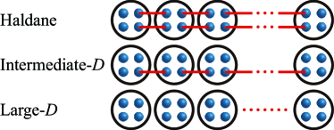
Figure 8: (Color online) Schematic pictures of $S=2$ Haldane, intermediate-$D$, and large-$D$ phases. The links connecting spin-1/2’s (balls) represent singlet bonds.

It is also worth pointing out that our theory is also closely related to the physics of the so-called intermediate-$D$ phase, which can arise in quantum spin chains with $S\geq 2$ in the presence of a single ion anisotropy term (without an external magnetic field). This phase is expected Oshikawa92 to lie in-between the Haldane gap phase (where, in the VBS picture, each one of the $2S$ auxiliary $S=1/2$ objects residing on a given site participates in the formation of a singlet bond with a neighboring site) and a trivial large-$D$ phase (where all $S=1/2$ objects are completely quenched out). In this phase, only a limited number of $S=1/2$ spins per site are involved in the VBS-like structure, while the others are quenched out due to the anisotropy term. For the $S=2$ case, numerical studies have verified that a phase transition exists between the intermediate-$D$ and Haldane phases [Fig. 8], while the Haldane and large-$D$ phases are connected within the phase diagram Tonegawa11 . The intermediate-$D$ phase is analogous to the situation encountered in the preceding discussions in the sense that (i) the fluctuation of the spins occur predominantly within the $xy$ plane (assuming the anisotropic term is of the form $D(S_{j}^{z})^{2}$), and that (ii) the effective local spin moment is depleted owing to those $S=1/2$ objects which do not participate in the singlet bonds. We thus expect that the low-energy physics is again captured by the planar limit of the O(3) NL$\sigma$ model at the vacuum angle $\theta=2\pi(S-m)$ where $m$ is now the amount of local spin moment that is quenched.

Finally we mention that the field theoretical approach of Secs. II and III also applies to the “Haldane insulators” in bosonic systems Fisher89 ; DallaTorre06 ; Batrouni13 . We start from a one-dimensional Bose-Hubbard model:

$${\cal H}_{\rm BH}=-t\sum_{j}(b_{j}^{\dagger}b_{j+1}+{\rm H.c.})+\frac{U}{2}\sum_{j}n_{j}(n_{j}-1)-\mu\sum_{j}n_{j},$$

where $b_{j}$, $b_{j}^{\dagger}$ are boson annihilation and creation operators, and $n_{j}\equiv b_{j}^{\dagger}b_{j}$ is a number operator. Switching to a coherent-state path integral language via the substitution $b_{j}(\tau)=\rho_{j}^{1/2}e^{i\phi_{j}(\tau)}$ and writing $\rho_{j}=\rho_{0}+\delta\rho_{j}$ ($\rho_{0}$ is the number of bosons per site), we obtain, upon integrating out $\delta\rho_{j}$ the effective Lagrangian Herbut07

$${\cal L}_{\rm BH}= \frac{1}{2U}\sum_{j}\big{(}\partial_{\tau}\phi_{j}(\tau)\big{)}^{2}-t\rho_{0}\sum_{j}\cos\big{[}\phi_{j}(\tau)-\phi_{j+1}(\tau)\big{]}$$

$$\quad+i\rho_{0}\sum_{j}\partial_{\tau}\phi_{j}(\tau).$$ (23)

In the continuum limit the kinetic terms (the first two terms on the right-hand side) in (23) assume the form

$${\cal L}_{\rm BH,kin}\sim\int dx\big{[}c_{\tau}\big{(}\partial_{\tau}\phi_{j}(\tau,x)\big{)}^{2}+c_{x}\big{(}\partial_{x}\phi_{j}(\tau,x)\big{)}^{2}\big{]},$$

where $c_{\tau}=1/(2Ua)$, $c_{x}=t\rho a/2$ ($a$ is the lattice constant). Moreover, the term $i\rho_{0}\sum_{j}\partial_{\tau}\phi_{j}(\tau)$ becomes identical with (5) upon the replacement $\rho_{0}\to S-m$. Therefore, the effective action for the Bose-Hubbard model takes the same form as (10). Essentially repeating the arguments of Secs. II and III, we are led to deduce that Haldane and trivial insulators in bosonic systems each correspond to $\rho_{0}=$ odd and even, and that the addition of a staggered chemical potential (which is the counterpart of the staggered magnetization of our previous discussion) will destroy this topological distinction.

Appendix A SPT phases protected by ${\rm U(1)}\rtimes Z_{2}^{\rm P}$ symmetry

The SPT phases protected by the symmetry ${\rm U(1)}\rtimes Z_{2}^{\rm P}$ is classified by the cohomology group $Z_{2}\times Z_{2}$, as can be read off from the classification table Chen12 for the mathematically equivalent entry ${\rm U(1)}\times Z_{2}^{\rm T}$. (Here $Z_{2}^{\rm T}$ and $Z_{2}^{\rm P}$ stand for time-reversal and link-parity symmetries, respectively.) One of these two $Z_{2}$ groups corresponds to whether $U_{\cal P}^{*}U_{\cal P}=+1$ or $-1$ as is discussed in the main text, where $U_{\cal P}$ is a unitary matrix corresponding to the projective representation of the link-parity operation ${\cal P}$:

$$\Gamma\xrightarrow{{\cal P}}\Gamma^{\text{T}}=e^{-i\theta_{\cal P}}U_{\cal P}\Gamma^{\rm T}U_{\cal P}^{\dagger}\;.$$ (24)

Next, let us find the projective representation of the U(1) group, which consists of rotations around the $z$ axis with angle $\alpha$ ($R_{z}^{(\alpha)}$) such as

$$R_{z}^{(\alpha)}\Gamma=e^{i\theta_{\alpha}}U_{z}^{(\alpha)\dagger}\Gamma U_{z}^{(\alpha)}.$$ (25)

We consider the effect of exchanging the order in which the two operators $R_{z}^{(\alpha)}$ and ${\cal P}$ act. From (24) and (25),

$$R_{z}^{(\alpha)}{\cal P}\Gamma= e^{i(\theta_{\cal P}+\theta_{\alpha})}U_{z}^{(\alpha)\dagger}U_{\cal P}^{\dagger}\Gamma U_{\cal P}U_{z}^{(\alpha)}$$

$${\cal P}R_{z}^{(\alpha)}\Gamma= e^{i(\theta_{\cal P}+\theta_{\alpha})}U_{\cal P}^{\dagger}(U_{z}^{(\alpha)\dagger}\Gamma U_{z}^{(\alpha)})^{\rm T}U_{\cal P}.$$

$$= e^{i(\theta_{\cal P}+\theta_{\alpha})}U_{\cal P}^{\dagger}U_{z}^{(\alpha){\rm T}}\Gamma U_{z}^{(\alpha)*}U_{\cal P}.$$

The relation $R_{z}^{(\alpha)}{\cal P}\Gamma={\cal P}R_{z}^{(\alpha)}\Gamma$ leads to

$$\Gamma=U_{\cal P}U_{z}^{(\alpha)}U_{\cal P}^{\dagger}U_{z}^{(\alpha){\rm T}}\Gamma U_{z}^{(\alpha)*}U_{\cal P}U_{z}^{(\alpha)\dagger}U_{\cal P}^{\dagger}.$$

Hence, $U_{\cal P}U_{z}^{(\alpha)}U_{\cal P}^{\dagger}U_{z}^{(\alpha){\rm T}}$ should be the left eigenvector of the transfer matrix and is equal to $e^{i\phi_{\alpha,{\cal P}}}E$ ($E$ is unit matrix). This implies that

$$U_{\cal P}U_{z}^{(\alpha)}=e^{i\phi_{\alpha,{\cal P}}}U_{z}^{(\alpha)*}U_{\cal P}.$$ (26)

Since the action of U(1) is diagonal ($U_{z}^{(\alpha){\rm T}}=U_{z}^{(\alpha)}$), $U_{z}^{(\alpha)*}=U_{z}^{(\alpha)\dagger}=U_{z}^{(\alpha)\;-1}=U_{z}^{(-\alpha)}$. Using this relation and (26), we can also derive

$$U_{z}^{(\alpha)}U_{\cal P}=e^{-i\phi_{\alpha,{\cal P}}}U_{\cal P}U_{z}^{(\alpha)*}$$ (27)

by the replacement $\alpha\to-\alpha$. From (26) and (27), $e^{i\phi_{\alpha,{\cal P}}}=\pm 1$ is proved, i.e., $U_{\cal P}U_{z}^{(\alpha)}=\pm U_{z}^{(\alpha)*}U_{\cal P}$. Therefore, the $Z_{2}\times Z_{2}$ classification of SPT phases protected by ${\rm U(1)}\rtimes Z_{2}^{\rm P}$ proceeds according to (i) $U_{\cal P}^{*}U_{\cal P}=+1$ or $-1$, and (ii) $U_{\cal P}U_{z}^{(\alpha)}=U_{z}^{(\alpha)*}U_{\cal P}$ or $U_{\cal P}U_{z}^{(\alpha)}=-U_{z}^{(\alpha)*}U_{\cal P}$.

For the SPT plateau state discussed in Sec. V (see Eq. (20)), the U(1) rotation acts as

$$R_{z}^{(\alpha)}\Gamma[3/2]=e^{3i\phi_{\alpha}/2}\Gamma[3/2],$$

$$R_{z}^{(\alpha)}\Gamma[1/2]=e^{i\phi_{\alpha}/2}\Gamma[1/2],$$

$$R_{z}^{(\alpha)}\Gamma[-1/2]=e^{-i\phi_{\alpha}/2}\Gamma[-1/2],$$

$$R_{z}^{(\alpha)}\Gamma[-3/2]=e^{-3i\phi_{\alpha}/2}\Gamma[-3/2].$$

We can find that

$$U_{z}^{(\alpha)}=e^{i\alpha\sigma^{z}/2},\quad\theta_{\alpha}=\alpha/2$$ (28)

satisfies Eq. (25). From (22) and (28), we can confirm that $U_{\cal P}U_{z}^{(\alpha)}=U_{z}^{(\alpha)*}U_{\cal P}$ holds. Therefore, the SPT plateau belongs to the category with (i) $U_{\cal P}^{*}U_{\cal P}=-1$ and (ii) $U_{\cal P}U_{z}^{(\alpha)}=U_{z}^{(\alpha)*}U_{\cal P}$. The search for SPT phases with $U_{\cal P}U_{z}^{(\alpha)}=-U_{z}^{(\alpha)*}U_{\cal P}$ is an interesting future problem.

References

- (1) X.-G. Wen, Quantum Field Theory of Many-Body Systems (Oxford University Press, Oxford, UK, 2004).
- (2) F. D. M. Haldane, Phys. Lett. A 93, 464 (1983); Phys. Rev. Lett. 50, 1153 (1983).
- (3) I. Affleck, T. Kennedy, E. H. Lieb, and H. Tasaki, Phys. Rev. Lett. 59, 799 (1987); Commun. Math. Phys. 115, 477 (1988).
- (4) M. P. Nightingale and H. W. J. Blöte, Phys. Rev. B 33, 659(R) (1986).
- (5) S. R. White and D. A. Huse, Phys. Rev. B 48, 3844 (1993).
- (6) E. Polizzi, F. Mila, and E. S. Sørensen, Phys. Rev. B 58, 2407 (1998).
- (7) K. Katsumata, H. Hori, T. Takeuchi, M. Date, A. Yamagishi, and J. P. Renard, Phys. Rev. Lett. 63, 86 (1989); Y. Ajiro, T. Goto, H. Kikuchi, T. Sakakibara, and T. Inami, ibid. 63, 1424 (1989).
- (8) F. Pollmann, A. M. Turner, E. Berg, and M. Oshikawa, Phys. Rev. B 81, 064439 (2010); F. Pollmann, E. Berg, A. M. Turner, and M. Oshikawa, ibid. 85, 075125 (2012).
- (9) X. Chen, Z.-C. Gu, and X.-G. Wen, Phys. Rev. B 84, 235128 (2011).
- (10) X. Chen, Z.-C. Gu, Z.-X. Liu, and X.-G. Wen, Science 338, 1604 (2012).
- (11) M. Levin and Z.-C. Gu, Phys. Rev. B 86, 115109 (2012).
- (12) Y.-M. Lu and A. Vishwanath, Phys. Rev. B 86, 125119 (2012).
- (13) T. Senthil and M. Levin, Phys. Rev. Lett. 110, 046801 (2013).
- (14) A. Vishwanath and T. Senthil, Phys. Rev. X 3, 011016 (2013).
- (15) P. Ye and X.-G. Wen, Phys. Rev. B 87, 195128 (2013).
- (16) E. H. Lieb, T. D. Schultz, and D. Mattis, Ann. Phys. (N. Y.) 16, 107 (1961).
- (17) M. Oshikawa, M. Yamanaka, and I. Affleck, Phys. Rev. Lett. 78, 1984 (1997).
- (18) K. Totsuka, Phys. Lett. A 228, 103 (1997).
- (19) A. Tanaka, K. Totsuka, and X. Hu, Phys. Rev. B 79, 064412 (2009).
- (20) H. Hu, C. Cheng, Z. Xu, H.-G. Luo, and S. Chen, Phys. Rev. B 90, 035150 (2014).
- (21) S. Takayoshi, M. Sato, and T. Oka, Phys. Rev. B 90, 214413 (2014).
- (22) S. Sachdev, Quantum Phase Transitions (Cambridge University Press, Cambridge, UK, 2011).
- (23) M. P. A. Fisher, P. B. Weichman, G. Grinstein, and D. S. Fisher, Phys. Rev. B 40, 546 (1989).
- (24) E. G. Dalla Torre, E. Berg, and E. Altman, Phys. Rev. Lett. 97, 260401 (2006).
- (25) G. G. Batrouni, R. T. Scalettar, V. G. Rousseau, and B. Grémaud, Phys. Rev. Lett. 110, 265303 (2013).
- (26) M. Endres, M. Cheneau, T. Fukuhara, C. Weitenberg, P. Schauß, C. Gross, L. Mazza, M. C. Bañuls, L. Pollet, I. Bloch, and S. Kuhr, Science 334, 200 (2011).
- (27) C. Xu and T. Senthil, Phys. Rev. B 87, 174412 (2013).
- (28) T.-K. Ng, Phys. Rev. B 50, 555 (1994).
- (29) S. Sachdev, Physica A 313, 252 (2002).
- (30) A. Auerbach, Interacting Electrons and Quantum Magnetism (Springer-Verlag, New York, 1994).
- (31) Similar discussions are made also for symmetry-protected trivial phases in, e.g., Y. Fuji, F. Pollmann, and M. Oshikawa, arXiv:1409.8616.
- (32) I. Affleck, J. Phys.: Condens. Matter 1, 3047 (1989).
- (33) G. Vidal, Phys. Rev. Lett. 98, 070201 (2007).
- (34) A. Kitazawa and K. Okamoto, Phys. Rev. B 62, 940 (2000).
- (35) H. J. Schulz, Phys. Rev. B 34, 6372 (1986).
- (36) W. Chen, K. Hida, and B. C. Sanctuary, Phys. Rev. B 67, 104401 (2003).
- (37) K. Hida, J. Phys. Soc. Jpn. 63, 2359 (1994).
- (38) H. Li and F. D. M. Haldane, Phys. Rev. Lett. 101, 010504 (2008).
- (39) T. Nishioka, S. Ryu, and T. Takayanagi, J. Phys. A: Math. Theor. 42, 504008 (2009).
- (40) Note that the lowest-energy state of Eq. (16) is highly degenerate. Infinitesimally small magnetic field splits the degeneracy and selects the state Eq. (15) as the unique (up to edge states) ground state with bulk magnetization 1/2. The single-mode approximation predicts a finite gap to the excitation that changes magnetization by 1. Therefore, the magnetization curve jumps at to and has a finite plateau there.
- (41) G. Vidal, Phys. Rev. Lett. 91, 147902 (2003).
- (42) D. Perez-Garcia, F. Verstraete, M. M. Wolf, and J. I. Cirac, Quantum Inf. Comput. 7, 401 (2007).
- (43) D. Perez-Garcia, M. M. Wolf, M. Sanz, F. Verstraete, and J. I. Cirac, Phys. Rev. Lett. 100, 167202 (2008).
- (44) M. Oshikawa, J. Phys.: Condens. Matter 4, 7469 (1992).
- (45) T. Tonegawa, K. Okamoto, H. Nakano, T. Sakai, K. Nomura, and M. Kaburagi, J. Phys. Soc. Jpn. 80, 043001 (2011).
- (46) I. Herbut, A Modern Approach to Critical Phenomena (Cambridge University Press, Cambridge, UK, 2007).