A kernel-based approach to Hammerstein system identification

Abstract

In this paper, we propose a novel algorithm for the identification of Hammerstein systems. Adopting a Bayesian approach, we model the impulse response of the unknown linear dynamic system as a realization of a zero-mean Gaussian process. The covariance matrix (or kernel) of this process is given by the recently introduced stable-spline kernel, which encodes information on the stability and regularity of the impulse response. The static nonlinearity of the model is identified using an Empirical Bayes approach—that is, by maximizing the output marginal likelihood, which is obtained by integrating out the unknown impulse response. The related optimization problem is solved adopting a novel iterative scheme based on the Expectation-Maximization method, where each iteration consists in a simple sequence of update rules. Numerical experiments show that the proposed method compares favorably with a standard algorithm for Hammerstein system identification.

1 Introduction

The Hammerstein system is a cascaded system composed of a static nonlinearity followed by a linear dynamic system (see e.g. [14]). Hammerstein system identification has become object of research apparently since the Sixties (see [16]). Due to the wide spectrum of applications (see e.g. [13], [23], [4]), Hammerstein system identification has gained popularity through the years and a wide range of methods has been developed (see [21], [2], [3], and references therein).

Several identification approaches have been proposed. For instance, [11] exploits kernel regression arguments, [23] uses a separable least squares approach, [10] focuses on stochastic system identification of Hammerstein models, while [9] proposes a subspace approach. Research on this topic is still rather active (see [22], [12]).

In this paper, we propose a novel method for Hammerstein system identification. Following recent developments in identification of linear dynamic systems (see [7], [20]), we adopt a kernel-based identification approach for the linear part of the Hammerstein model. To this end, we model the impulse response of the unknown linear system as a realization of a Gaussian process. The covariance matrix (or kernel) of this process has a specific structure given by the stable spline kernel (see [19], [18], [5]). This structure induces properties such as BIBO stability and smoothness in the Gaussian process realizations and depends on a shaping parameter which regulates the exponential decay of the generated impulse responses.

In the context of Hammerstein system identification, we can define an effective estimator of the linear dynamic block using Bayesian arguments by exploiting the kernel-based framework. Such an estimator is function of the static nonlinearity, as well as the kernel shaping parameter and the noise variance. A crucial point of the proposed approach is the estimation of these quantities. Exploiting a Bayesian interpretation of kernel-based methods  [15], we perform this estimation step by maximizing the marginal likelihood of the output measurements, which is obtained by integrating out the unknown impulse response. This approach has been shown to be effective in kernel-based linear system identification  [17]. However, when applied to Hammerstein system identification, the related optimization problem becomes more involved due to the presence of the unknown static nonlinearity. To overcome this difficulty, we propose a novel iterative solution scheme based on the Expectation-Maximization method proposed by [8]. We show that the resulting Hammerstein system identification algorithm has a rather low computational burden. Remarkably, the proposed method does not need any parameter to be set nor requires the user to select the model order of the linear system. This in contrast with standard parametric methods, where, when little is known about the system, one as to estimate the optimal model order using complexity criteria or cross validation (see e.g. [14]).

The method used in this paper is also used in [6] in the context of blind system-identification.

The structure of the paper is as follows. In the next section, we formulate the Hammerstein system identification problem. In Section 3, we describe the model adopted for the linear system and the static nonlinearity. In Section 4, we introduce the proposed algorithm, which is tested in Section 5. Some conclusions end the paper.

2 Problem formulation

We consider a single input single output discrete-time system described by the following time-domain relations (see Figure 1)

$$\begin{array}[]{lcl}w_{t}&=&f(u_{t})\\ y_{t}&=&\sum_{k=1}^{\infty}g_{k}w_{t-k}+e_{t}\,.\end{array}$$ (1)

In the above equation, $f(\cdot)$ represents a (static) nonlinear function transforming the measurable input $u_{t}$ into the unavailable signal $w_{t}$, which in turn feeds a linear time-invariant (LTI) strictly causal system described by the impulse response $g_{t}$. The output measurements of the system $y_{t}$ are corrupted by white Gaussian noise, denoted by $e_{t}$, which has unknown variance $\sigma^{2}$. For simplicity, we assume null initial conditions.

Figure 1: Block scheme of the Hammerstein system.

We assume that $N$ input-output samples are collected, and denote them by ${\{u_{t}\}}_{t=0}^{N-1}$, $i{\{y_{t}\}}_{t=1}^{N}$. For notational convenience, we also assume null initial conditions. Then, the system identification problem we discuss in this paper is the problem of estimating $n$ samples of the impulse response say, ${\{\hat{g}_{t}\}}_{t=1}^{n}$ (where $n$ is large enough to capture the system dynamics), as well as the static nonlinearity $f(\cdot)$.

Remark 1

The identification method we propose in this paper is not affected by the choice of $n$. Furthermore, it can be derived also in the continuous-time setting, using the same arguments as in [19]. However, for ease of exposition, here we focus only on the discrete-time case.

2.1 Non-uniqueness of the identified system

It is well-known (see e.g. [3]) that the two components of a Hammerstein system can be determined up to a scaling factor. In fact, for every $\alpha\in\mathbb{R}$, the pair $(\alpha g_{t},\,\frac{1}{\alpha}f(\cdot))$, describes the input-output relation equally well. We will address this issue in the modeling of the impulse response by fixing the kernel scaling parameter (see Subsection 3.3).

3 Modeling and identification of Hammerstein Systems

In this section, we first introduce the models adopted for the input static nonlinearity and the LTI system. Then, we describe the proposed system identification method.

3.1 Notation

Let us introduce the vector-based notation

$$u\triangleq\begin{bmatrix}u_{0}\\ \vdots\\ u_{N-1}\end{bmatrix},\,y\triangleq\begin{bmatrix}y_{1}\\ \vdots\\ y_{N}\end{bmatrix},\,g\triangleq\begin{bmatrix}g_{1}\\ \vdots\\ g_{n}\end{bmatrix},\,e\triangleq\begin{bmatrix}e_{1}\\ \vdots\\ e_{N}\end{bmatrix}.$$

Furthermore, we define the operator $\mathbf{T}_{n}(\cdot)$ that, given a vector of length $N$, maps it to an $N\times n$ Toeplitz matrix:

$$\mathbf{T}_{n}(w)=\begin{bmatrix}w_{0}&0&&\cdots&0\\ w_{1}&w_{0}&0&\cdots&0\\ \vdots&\vdots&&\ddots&\vdots\\ w_{N-2}&w_{N-3}&\cdots&w_{N-n+1}&0\\ w_{N-1}&w_{N-2}&\cdots&\cdots&w_{N-n}\end{bmatrix}\,\in\,\mathbb{R}^{N\times n}\,.$$

We shall reserve the symbol $W$ for $\mathbf{T}_{n}(w)$. This allows us to write the input-output relation of the LTI system as

$$y=Wg+e\,.$$ (2)

3.2 The input static nonlinearity

Following [2], [3], we assume that the input static nonlinearity belongs to a $p$-dimensional space of functions and thus can be described using a linear combination of known basis functions ${\{\phi_{i}\}}_{i=1}^{p}$. Hence, we can write

$$w_{t}=f(u_{t})=\sum_{i=1}^{p}c_{i}\phi_{i}(u_{t})\,,$$ (3)

where the coefficients $c_{i}$ are unknown. The problem of estimating $f(\cdot)$ is thus equivalent to the problem of determining such coefficients. By introducing the following matrix

$$F(u)\triangleq\begin{bmatrix}\phi_{1}(u_{0})&\cdots&\phi_{p}(u_{0})\\ \vdots&\vdots&\vdots\\ \phi_{1}(u_{N-1})&\cdots&\phi_{p}(u_{N-1})\\ \end{bmatrix}$$ (4)

we can write

$$w=F(u)c\,,$$ (5)

where $c\triangleq\begin{bmatrix}c_{1}&\cdots&c_{p}\end{bmatrix}^{T}$.

3.3 Kernel-based modeling of the LTI system

In this paper, we adopt the kernel-based identification approach for LTI systems, proposed in [19], [18]. To this end, following a Gaussian process regression approach [24], we assume that the impulse response of the system is a realization of a zero-mean Gaussian process, namely

$$g\sim\mathcal{N}(0,\lambda K_{\beta})\,.$$ (6)

The matrix $K_{\beta}$, which is also known as kernel, is a covariance matrix parameterized by a shaping parameter $\beta$, and $\lambda\geq 0$ is a scaling factor. In the context of system identification, the family of the stable spline kernels [19], [18]itutes a valid choice, since they promote BIBO stable and smooth realizations. Specifically, we employ the first-order stable spline kernel (or TC kernel in [7]) given by

$${\{K_{\beta}\}}_{i,j}\triangleq\beta^{\max(i,j)}\,,\quad 0\leq\beta<1$$ (7)

where $\beta$ determines the decaying velocity of the generated impulse responses. As $\lambda$ regulates the amplitude of the impulse response $g$, we can we can arbitrarily set $\lambda=1$, to cope with the identifiability issue described in Section 2.1.

3.4 Estimation of the LTI system

In this section we derive the system identification strategy that arises naturally when kernel-based methods are employed. The estimator we will obtain is function of the vector

$$\theta\triangleq\begin{bmatrix}c^{T}&\sigma^{2}&\beta\end{bmatrix}\quad\in\mathbb{R}^{p+2}\,,$$ (8)

which we shall call hyperparameter vector. Since the noise is assumed Gaussian, the joint distribution of the vectors $y$ and $g$ is again Gaussian, and parametrized by $\theta$. Thus

$$p\left(\begin{bmatrix}y\\ g\end{bmatrix};\theta\right)\sim\mathcal{N}\left(\begin{bmatrix}0\\ 0\end{bmatrix},\begin{bmatrix}\Sigma_{y}&\Sigma_{yg}\\ \Sigma_{gy}&K_{\beta}\end{bmatrix}\right)\,,$$ (9)

where $\Sigma_{yg}=\Sigma_{gy}^{T}=WK_{\beta}$ and $\Sigma_{y}=WK_{\beta}W^{T}+\sigma^{2}I$. It follows that the posterior distribution of $g$ given $y$ is also Gaussian:

$$p(g|y;\,\theta)=\mathcal{N}\left(Cy,\,P\right)\,,$$ (10)

where

$$P={\left(\frac{W^{T}W}{\sigma^{2}}+K_{\beta}^{-1}\right)}^{-1}\quad,\quad C=P\frac{W^{T}}{\sigma^{2}}\,.$$ (11)

The hyperparameter vector $\theta$ needs to be estimated from the available data, and we will address this point in the next section.

Given a value of $\theta$, from (10), we find the impulse response estimator as the minimum mean squared error estimator [1]

$$\hat{g}=\mathbb{E}[g|y;\,\theta]=Cy\,.$$ (12)

4 Empirical Bayes estimates of the parameters

In this section we deal with the estimation of the hyperparameter vector $\theta$. Exploiting the Bayesian framework introduced in the previous section, we adopt an Empirical Bayes approach [15] for this task. The hyperparameter vector is obtained by maximizing the marginal likelihood of the output:

$$\begin{split}\hat{\theta}&=\arg\max_{\theta}\log p(y;\theta)\\ &=\arg\min_{\theta}\log\det\Sigma_{y}+y^{T}\Sigma_{y}^{-1}y.\end{split}$$ (13)

4.1 Solution via the EM method

Problem (13) is non-convex and nonlinear, and involves $p+2$ decision variables. For its solution, we propose a scheme based on the EM method. To this end, we introduce the complete-data log-likelihood

$$L(y,\,g;\theta)\triangleq\log p(y,\,g;\theta)\,,$$ (14)

where $g$ plays the role of latent variable. The EM method solves (13) by iteratively marginalizing out $g$ from (14). This operation is performed by iterating the following steps:

(E-step)

At the $k$-th iteration, using the estimate $\hat{\theta}^{(k)}$, compute

$$\mathcal{Q}(\theta,\,\hat{\theta}^{(k)})\triangleq\mathbb{E}_{p(g;y,\,\hat{\theta}^{(k)})}\left[L(y,\,g;\theta)\right]\,;$$ (15)

(M-step)

update the the estimate solving

$$\hat{\theta}^{(k+1)}=\arg\max_{\theta}\mathcal{Q}(\theta,\,\hat{\theta}^{(k+1)})\,.$$ (16)

Such a procedure converges to a maximum (not necessarily global) of (13) (see e.g. [mclachlan2007maximum]).

Let us assume that the estimate $\hat{\theta}^{(k)}$ of the hyperparameter vector has been computed at the $k$-th iteration of the EM method. Using (11), we can compute the quantities $\hat{P}^{(k)}$ and $\hat{m}_{g}^{(k)}$, namely the posterior mean and variance of $g$ given $y$. The following theorem illustrates how to compute $\hat{\theta}^{(k+1)}$.

Theorem 1

Assume that $\hat{\theta}^{(k)}$ is available. Then, the updated estimate

$$\hat{\theta}^{(k+1)}=\begin{bmatrix}\hat{c}^{(k+1)T}&\hat{\sigma}^{2,(k+1)}&\hat{\beta}^{(k+1)}\end{bmatrix}$$ (17)

is obtained by means of the following steps:

• The coefficients of the nonlinear block are given by

  $$\hat{c}^{(k+1)}={(\hat{A}^{(k)})}^{-1}\hat{b}^{(k)}\,,$$ (18)

  where

  $$\begin{split}\hat{A}^{(k)}&={F(u)}^{T}\mathbf{R}^{T}\big{(}(\hat{P}^{(k)}+\hat{m}_{g}^{(k)}\hat{m}_{g}^{(k)\,T})\otimes I_{N}\big{)}\mathbf{R}F(u)\,,\\ \hat{b}^{(k)}&={F(u)}^{T}\mathbf{T}_{N}\big{(}\hat{m}_{g}^{(k)}\big{)}y\,,\end{split}$$ (19)

  where $\mathbf{R}\in\mathbb{R}^{Nn\times N}$ is the (unique) matrix such that, for all $u\in\mathbb{R}^{N}$, we have

  $$\mathbf{R}u=\mathrm{vec}\big{(}\mathbf{T}_{n}(u)\big{)};$$ (20)

• The noise variance is updated using

  $$\begin{split}\hat{\sigma}^{2,(k+1)}&=\frac{1}{N}\Big{(}\|y-\hat{W}^{(k+1)}\hat{m}_{g}^{(k)}\|^{2}_{2}\\ &+\mathrm{Tr}\{\hat{W}^{(k+1)}\hat{P}^{(k)}\hat{W}^{(k+1)T}\}\Big{)}\end{split}$$ (21)

  where $\hat{W}^{(k+1)}=\mathbf{T}_{n}\big{(}F(u)\hat{c}^{(k+1)}\big{)}$ results by plugging the new estimates $\hat{c}^{(k+1)}$ in (5);

• The updated kernel shaping parameter is solution of

  $$\hat{\beta}^{(k+1)}=\arg\max_{\beta}Q_{\beta}(\beta,\hat{\theta}^{(k)})\,,$$ (22)

  where

  $$Q_{\beta}(\beta,\hat{\theta}^{(k)})\triangleq\log\det K_{\beta}+\mathrm{Tr}\Big{[}K_{\beta}^{-1}\big{(}\hat{P}^{(k)}+\hat{m}_{g}^{(k)}\hat{m}_{g}^{(k)T}\big{)}\Big{]}.$$ (23)

Therefore, the solution of (13) can be retrieved in a simple and quick way. In fact, Theorem 1 states that, given an estimate of the hyperparameter vector, the updated values of the coefficients of the nonlinear block are obtained solving a system of linear equations. Then, the new estimate of the noise variance can also be computed using a closed-form expression. Finally, the new value of the kernel shaping parameter is retrieved by solving a simple optimization problem. Although such a problem does not seem to admit a closed-form solution, we note that it is a one dimensional problem in the domain $[0,\,1]$. Hence, it can be quickly solved by pointwise evaluation.

Below, we give our novel kernel based method for the identification of Hammerstein systems.

Algorithm: Kernel-based Hammerstein System Identification
Input: ${\{u_{t}\}}_{t=0}^{N-1}$, ${\{y_{t}\}}_{t=1}^{N}$
Output: ${\{\hat{g}\}}_{t=1}^{n}$, $\hat{f}(\cdot)$

1. Initialization: randomly set $\hat{\theta}^{(0)}$

2. Repeat until convergence:

   1. E-step: update $\hat{P}^{(k)}$, $\hat{C}^{(k)}$ from (11) and $\hat{m}_{g}^{(k)}$ from (12);

   2. M-step: update the parameters:

      • $\hat{c}^{(k+1)}$ from (18);

      • $\hat{\sigma}^{(k+1)}$ from (21),

      • $\hat{\beta}^{(k+1)}$ from (22)

3. Compute ${\{\hat{g}\}}_{t=1}^{n}$ from (12) and $\hat{f}(\cdot)=\sum_{i=1}^{p}\hat{c}_{i}\phi_{i}(\cdot)$;

Remark 2

The choice of random initial is motivated by the fact that, after several numerical experiments we have noticed that the algorithm is capable of reaching the global maximum of (13) independently of the initial conditions.

5 Numerical Experiments

In order to assess the performance of the proposed Hammerstein system identification scheme, we run a set of Monte Carlo experiments. Specifically, we perform 8 different identification experiments, each consisting of 100 independent Monte Carlo runs. Depending on the experiment, we generate systems of order $\nu$, where $\nu=4,\,8,\,10,\,20$. At each Monte Carlo run, a system is generated by picking $\nu$ random poles and zeros. The poles and zeros are located in the set $\{z\in\mathbb{C}\mbox{ s.t. }0.4\leq z\leq 0.93\}$. The input nonlinearity is chosen to be a polynomial of sixth order, so that $\phi_{i}(u)=u^{i-1}$, $i=1,\,\ldots,\,7$. The roots of the polynomial are in random locations within the interval $[-2,2]$. The input to the system is white noise, with uniform distribution in the same interval. We generate $N=500$ input/output samples for any Monte Carlo run. The output is corrupted by Gaussian white noise whose variance is chosen so to obtain a certain signal to noise ratio, according to

$$\sigma^{2}=\frac{\mathrm{Var}\left\{Wg\right\}}{\mathrm{SNR}}\,,$$ (24)

where $\mathrm{SNR}$ is either 10 or 1, depending on the experiment. The features of the 8 experiments are summarized in Table 1.

Experiment $\#$	1	2	3	4	5	6	7	8
LTI System Order	4	8	10	20	4	8	10	20
SNR	10	10	10	10	1	1	1	1

Table 1: Features of the 8 Monte Carlo experiments performed to test the proposed method.

The goal of the experiments is to estimate $n=100$ samples of the impulse response of the LTI system and the $p=7$ coefficients of the nonlinear block. In order to obtain uniqueness in the decompositions, we impose $\|g\|_{2}=1$, and we assume the sign of the first nonzero element of $g$ to be known.

We compare the following two estimators:

• KB-H This is the proposed kernel-based Hammerstein system identification method, which estimates the prior shaping parameter $\beta$, the nonlinear function and the noise variance through marginal likelihood maximization and the EM method. The convergence criterion for the EM method is $\|\hat{\theta}^{(k+1)}-\hat{\theta}^{(k)}\|_{2}<10^{-3}$.

• NLHW This is the matlab function nlhw that uses the prediction error method to identify the linear block in the system (see [Ljung2009toolbox] for details). To get the best performance from this method, we equip it with an oracle that knows the true order of the LTI system generating the measurements.

We use two metrics to evaluate the performance of the estimators. We consider the fitting score of the system impulse response

$$FIT_{g,i}=1-\frac{\left\|g_{i}-\hat{g}_{i}\right\|_{2}}{\left\|g_{i}-\bar{g}_{i}\right\|_{2}}\,,$$ (25)

where $g_{i}$ is the system generated at the $i$-th run of each experiment, $\hat{g}_{i}$ its estimate and $\bar{g}_{i}$ its mean. A similar fitting score is defined for the nonlinearity, namely

$$FIT_{f,i}=1-\frac{\|f_{i}(u)-\hat{f}_{i}(u)\|_{2}}{\|f_{i}(u)-\overline{f_{i}(u)}\|_{2}}\,.$$ (26)

Figure 2 shows one Monte Carlo realization with LTI system order equal to 10 and SNR $=10$, while Figure 3 shows the results of the outcomes of the 8 experiments. The box-plots compare the results of KB and NLHW for the considered model orders. We can see that, for low model orders, the estimator NLHW equipped with the true model order outperforms the proposed method. For higher model orders, however, the proposed method KB-H gives substantially better performance than NLHW. The reason is that KB-H is not affected by the increasing complexity (model order) of the system, and the fitting score remains approximately constant. In addition, we can notice that the estimation of the nonlinear block computed with KB-H always provides a higher accuracy than NLHW.

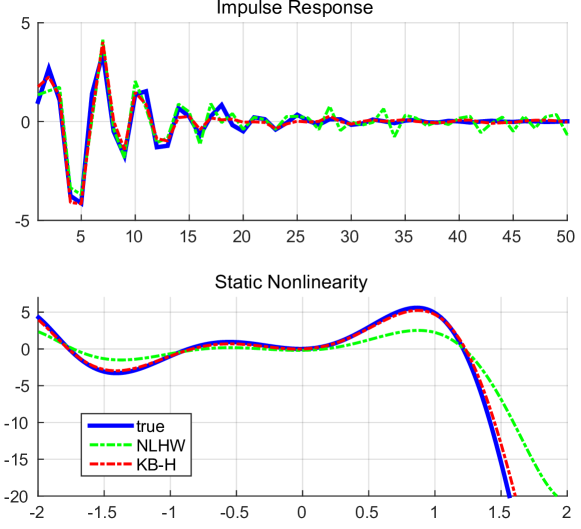
Figure 2: Realizations of one Monte Carlo run with LTI system order 10 and SNR $=10$.

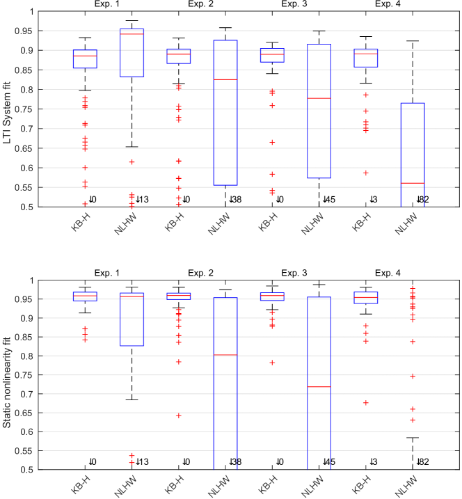
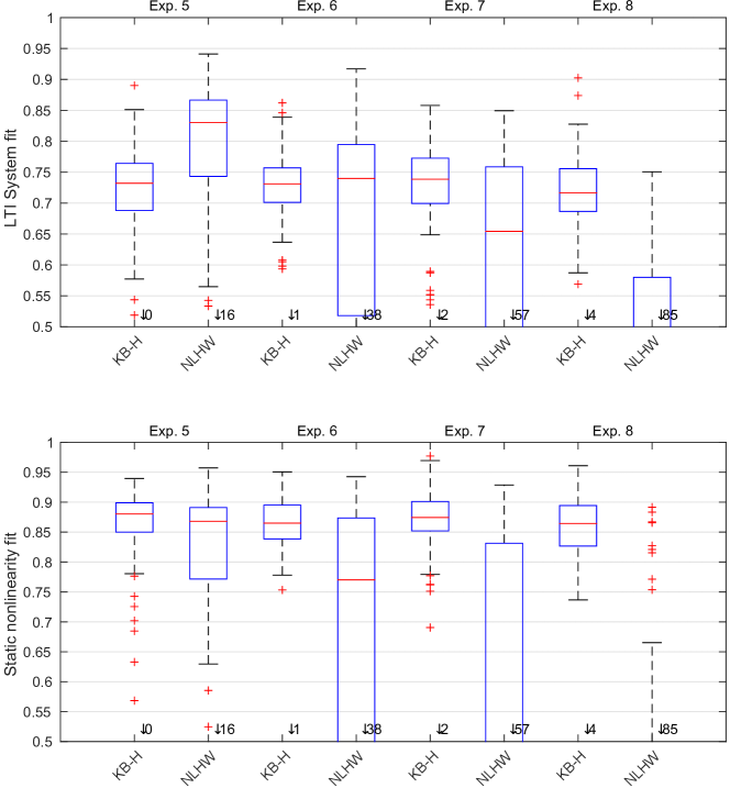
Figure 3: Results of the 8 Monte Carlo experiments summarized in Table 1.

6 Conclusions

In this work, we have proposed a novel kernel-based approach to the identification of Hammerstein dynamic systems. To model the impulse response we have adopted a Gaussian regression approach and employed the stable spline kernel. The identification of the input nonlinearity, together with the kernel hyperparameter and the noise variance, has been performed using an empirical Bayes approach. The related marginal likelihood maximization has been carried out resorting to the EM method. We have shown that this approach leads to an iterative scheme consisting of a set of simple update rules, which allow for fast computation. The effectiveness of the proposed method has been tested by means of several numerical experiments. When compared with standard state-of-the-art algorithms, the proposed method has shown a better fitting capacity in both the nonlinear block and the LTI system impulse response.

We are currently working on the extension of the algorithm to a wider class of system models. Furthermore, nonparametric descriptions of the nonlinear function will be considered in order to obtain a completely parameter-free identification method.

Appendix A Proof of Theorem 1

The proof runs along the same arguments as the proof of Theorem 1 in [6] and is included here for the sake of self-completeness.

Using the conditional probability formula,

$$p(y,\,g;\,\theta)=p(y|g;\,\theta)p(g;\,\theta)\,.$$ (27)

we can write the complete-data log-likelihood (14) as

$$L(y,\,g;\,\theta)=\log p(y|g;\,\theta)+\log p(g;\,\theta)$$ (28)

and so

$$L(y,\,g;\,\theta) =-\frac{N}{2}\log\sigma^{2}-\frac{1}{2\sigma^{2}}\left\|y-Wg\right\|^{2}\allowdisplaybreaks[1]-\frac{1}{2}\log\det K_{\beta}-\frac{1}{2}g^{T}K_{\beta}^{-1}g\allowdisplaybreaks[1]$$

$$=-\frac{N}{2}\log\sigma^{2}-\frac{1}{2\sigma^{2}}\left(y^{T}y+g^{T}W^{T}Wg-2y^{T}Wg\right)\allowdisplaybreaks[1]$$

$$\qquad\quad-\frac{1}{2}\log\det K_{\beta}-\frac{1}{2}g^{T}K_{\beta}^{-1}g\allowdisplaybreaks[1]\,.$$

We now proceed by taking the expectation of this expression with respect to the random variable $g|y;\,\hat{\theta}^{(k)}$. We obtain the following components

$$(a) :\mathbb{E}\left[-\frac{N}{2}\log\sigma^{2}\right]\!=\!-\frac{N}{2}\log\sigma^{2}\allowdisplaybreaks[1]$$

$$(b) :\mathbb{E}\left[-\frac{1}{2\sigma^{2}}y^{T}y\right]\!=\!-\frac{1}{2\sigma^{2}}y^{T}y\allowdisplaybreaks[1]$$

$$(c) :\mathbb{E}\left[-\frac{1}{2\sigma^{2}}g^{T}W^{T}Wg\right]=$$

$$\qquad\qquad\qquad\mathrm{Tr}\left[-\frac{1}{2\sigma^{2}}W^{T}W(\hat{P}^{(k)}\!+\!\hat{m}_{g}^{(k)}\hat{m}_{g}^{(k)T})\right]\allowdisplaybreaks[1]$$

$$(d) :\mathbb{E}\left[\frac{1}{\sigma^{2}}y^{T}Wg\right]\!=\!\frac{1}{\sigma^{2}}y^{T}W\hat{m}_{g}^{(k)}\allowdisplaybreaks[1]$$

$$(e) :\mathbb{E}\left[-\frac{1}{2}\log\det K_{\beta}\right]\!=\!-\frac{1}{2}\log\det K_{\beta}\allowdisplaybreaks[1]$$

$$(f) :\mathbb{E}\left[-\frac{1}{2}g^{T}K_{\beta}^{-1}g\right]=-\frac{1}{2}\mathrm{Tr}\left[K_{\beta}^{-1}(\hat{P}^{(k)}+\hat{m}_{g}^{(k)}\hat{m}_{g}^{(k)T})\right]$$

It follows that $Q(\theta,\,\hat{\theta}^{(k)})$ is the summation of the elements obtained above. By inspecting the structure of $Q(\theta,\,\hat{\theta}^{(k)})$, it can be seen that such a function splits in two independent terms, namely

$$\mathcal{Q}(\theta,\,\hat{\theta}^{(k)})=\mathcal{Q}_{1}(c,\,\sigma^{2},\,\hat{\theta}^{(k)})+\mathcal{Q}_{\beta}(\beta,\,\hat{\theta}^{(k)})\,,$$ (29)

where

$$\mathcal{Q}_{1}(c,\,\sigma^{2},\,\hat{\theta}^{(k)})=(a)+(b)+(c)+(d)$$ (30)

is function of $c$ and $\sigma^{2}$, while

$$\mathcal{Q}_{\beta}(\beta,\,\hat{\theta}^{(k)})=(e)+(f)$$ (31)

depends only on $\beta$ and corresponds to (23). We now address the optimization of (30). To this end we write

$$\mathcal{Q}_{1}(c,\sigma^{2},\,\hat{\theta}^{(k)}) =\frac{1}{\sigma^{2}}\mathcal{Q}_{c}(c,\,\hat{\theta}^{(k)})+\mathcal{Q}_{\sigma^{2}}(\sigma^{2},\,\hat{\theta}^{(k)})$$ (32)

$$=\frac{1}{\sigma^{2}}\Big{(}\mathrm{Tr}\left[-\frac{1}{2}W^{T}W(\hat{P}^{(k)}+\hat{m}_{g}^{(k)}\hat{m}_{g}^{kT})\right]$$

$$+y^{T}W\hat{m}_{g}^{(k)}\Big{)}-\frac{N}{2}\log\sigma^{2}-\frac{1}{2\sigma^{2}}y^{T}y$$

This means that the optimization of $\mathcal{Q}_{1}$ can be carried out first with respect to $c$, optimizing only the term $\mathcal{Q}_{c}$, which is independent of $\sigma^{2}$ and can be written in a quadratic form

$$\mathcal{Q}_{c}(c,\,\hat{\theta}^{(k)})=-\frac{1}{2}c^{T}\hat{A}^{(k)}c+\hat{b}^{(k)T}c\,.$$ (33)

To this end, first note that, for all $v_{1}\in\mathbb{R}^{n}$, $v_{2}\in\mathbb{R}^{m}$:

$$\mathbf{T}_{m}(v_{1})v_{2}=\mathbf{T}_{n}(v_{2})v_{1}\,.$$ (34)

Recalling (20), we can write

$$\begin{split}&-\frac{1}{2}\mathrm{Tr}\left[W^{T}W(\hat{P}^{(k)}\!\!+\!\!\hat{m}_{g}^{(k)}\hat{m}_{g}^{(k)T})\right]\\ &=-\frac{1}{2}{\mathrm{vec}(W)}^{T}\!((\hat{P}^{(k)}\!\!+\!\!\hat{m}_{g}^{(k)}\hat{m}_{g}^{(k)T})\otimes I_{N})\mathrm{vec}(W)\\ &=-\frac{1}{2}w^{T}\mathbf{R}^{T}\left((\hat{P}^{(k)}+\hat{m}_{g}^{(k)}\hat{m}_{g}^{(k)T})\otimes I_{N}\right)\mathbf{R}w\\ &=-\frac{1}{2}c^{T}{F(u)}^{T}\mathbf{R}^{T}\left((\hat{P}^{(k)}+\hat{m}_{g}^{(k)}\hat{m}_{g}^{(k)T})\otimes I_{N}\right)\mathbf{R}F(u)c\,,\end{split}$$

where the matrix in the middle corresponds to $\hat{A}^{(k)}$ defined in (19). For the linear term we find

$$y^{T}W\hat{g}^{(k)}=y^{T}\mathbf{T}_{N}(\hat{m}_{g}^{(k)})w=y^{T}\mathbf{T}_{N}(\hat{m}_{g}^{(k)})F(u)c\,,$$ (35)

so that the term $\hat{b}^{(k)T}$ in (19) is retrieved and the maximizer $\hat{c}^{(k+1)}$ is as in (18). Plugging back $\hat{c}^{(k+1)}$ into (30) and maximizing with respect to $\sigma^{2}$ we easily find $\hat{\sigma}^{2,(k+1)}$ corresponding to (21). This concludes the proof.

References

- [1] B. D. O. Anderson and J. B. Moore “Optimal filtering” Courier Corporation, 2012
- [2] E. W. Bai “An optimal two-stage identification algorithm for Hammerstein–Wiener nonlinear systems” In Automatica 34.3, 1998, pp. 333–338
- [3] E. W. Bai and D. Li “Convergence of the iterative Hammerstein system identification algorithm” In IEEE Trans. Autom. Control 49.11 IEEE, 2004, pp. 1929–1940
- [4] E. W. Bai, Z. Cai, S. Dudley-Javorosk and R.K. Shields “Identification of a modified Wiener–Hammerstein system and its application in electrically stimulated paralyzed skeletal muscle modeling” In Automatica 45.3 Elsevier, 2009, pp. 736–743
- [5] G. Bottegal and G. Pillonetto “Regularized spectrum estimation using stable spline kernels” In Automatica 49.11 Elsevier, 2013, pp. 3199–3209
- [6] Giulio Bottegal, Riccardo S Risuleo and Håkan Hjalmarsson “Blind system identification using kernel-based methods” In Proc. IFAC Symp. System Identification (SYSID) 48.28, 2015, pp. 466–471 DOI: doi:10.1016/j.ifacol.2015.12.172
- [7] T. Chen, H. Ohlsson and L. Ljung “On the estimation of transfer functions, regularizations and Gaussian processes—Revisited” In Automatica 48.8 Elsevier, 2012, pp. 1525–1535 DOI: 10.1016/j.automatica.2012.05.026
- [8] A. P. Dempster, N. M. Laird and D. B. Rubin “Maximum likelihood from incomplete data via the EM algorithm” In J. R. Stat. Soc. Ser. B. Stat. Methodol. JSTOR, 1977, pp. 1–38
- [9] I. Goethals, K. Pelckmans, J.A.K. Suykens and B. De Moor “Subspace identification of Hammerstein systems using least squares support vector machines” In IEEE Trans. Autom. Control 50.10 IEEE, 2005, pp. 1509–1519
- [10] W. Greblicki “Stochastic approximation in nonparametric identification of Hammerstein systems” In IEEE Transactions on Automatic Control 47.11 Institute of Electrical & Electronics Engineers (IEEE), 2002, pp. 1800–1810 DOI: 10.1109/tac.2002.804483
- [11] W. Greblicki and M. Pawlak “Identification of discrete Hammerstein systems using kernel regression estimates” In IEEE Trans. Autom. Control 31.1 IEEE, 1986, pp. 74–77
- [12] Y. Han and R.A. De Callafon “Hammerstein system identification using nuclear norm minimization” In Automatica 48.9 Elsevier, 2012, pp. 2189–2193
- [13] I.W. Hunter and M.J. Korenberg “The identification of nonlinear biological systems: Wiener and Hammerstein cascade models” In Biol. Cybern. 55.2-3 Springer, 1986, pp. 135–144
- [14] L. Ljung “System Identification, Theory for the User” Prentice Hall, 1999
- [15] J.S. Maritz and T. Lwin “Empirical bayes methods” ChapmanHall London, 1989
- [16] K. Narendra and P. Gallman “An iterative method for the identification of nonlinear systems using a Hammerstein model” In IEEE Transactions on Automatic Control 11.3 Institute of Electrical & Electronics Engineers (IEEE), 1966, pp. 546–550 DOI: 10.1109/tac.1966.1098387
- [17] G. Pillonetto and A. Chiuso “Tuning complexity in kernel-based linear system identification: The robustness of the marginal likelihood estimator” In Proc. European Control Conf. (ECC), 2014, pp. 2386–2391 DOI: 10.1109/ECC.2014.6862629
- [18] G. Pillonetto and G. De Nicolao “Kernel selection in linear system identification Part I: A Gaussian process perspective” In Proc. IEEE Conf. Decis. Control - European Control Conf. (CDC-ECC), 2011, pp. 4318–4325 DOI: 10.1109/CDC.2011.6160606
- [19] Gianluigi Pillonetto and Giuseppe De Nicolao “A new kernel-based approach for linear system identification” In Automatica 46.1 Elsevier, 2010, pp. 81–93
- [20] Gianluigi Pillonetto et al. “Kernel methods in system identification, machine learning and function estimation: A survey” In Automatica 50.3 Elsevier BV, 2014, pp. 657–682 DOI: 10.1016/j.automatica.2014.01.001
- [21] S. Rangan, G. Wolodkin and K. Poolla “New results for Hammerstein system identification” In Proc. IEEE Conf. Decis. Control (CDC) 1, 1995, pp. 697–702 IEEE
- [22] Maarten Schoukens, Rik Pintelon and Yves Rolain “Parametric Identification of Parallel Hammerstein Systems” In IEEE Trans. Instrum. Meas. 60.12 Institute of Electrical & Electronics Engineers (IEEE), 2011, pp. 3931–3938 DOI: 10.1109/tim.2011.2138370
- [23] D.T. Westwick and R.E. Kearney “Separable least squares identification of nonlinear Hammerstein models: Application to stretch reflex dynamics” In Ann. Biomed. Eng. 29.8 Springer, 2001, pp. 707–718
- [24] C.K. Williams and C.E. Rasmussen “Gaussian processes for machine learning” In the MIT Press, 2006