AGB SODIUM ABUNDANCES IN THE GLOBULAR CLUSTER 47 TUCANAE (NGC 104)

Abstract

A recent analysis comparing the [Na/Fe] distributions of red giant branch (RGB) and asymptotic giant branch (AGB) stars in the Galactic globular cluster NGC 6752 found that the ratio of Na–poor to Na–rich stars changes from 30:70 on the RGB to 100:0 on the AGB. The surprising paucity of Na–rich stars on the AGB in NGC 6752 warrants additional investigations to determine if the failure of a significant fraction of stars to ascend the AGB is an attribute common to all globular clusters. Therefore, we present radial velocities, [Fe/H], and [Na/Fe] abundances for 35 AGB stars in the Galactic globular cluster 47 Tucanae (47 Tuc; NGC 104), and compare the AGB [Na/Fe] distribution with a similar RGB sample published previously. The abundances and velocities were derived from high resolution spectra obtained with the Michigan/Magellan Fiber System (M2FS) and MSpec spectrograph on the Magellan–Clay 6.5m telescope. We find the average heliocentric radial velocity and [Fe/H] values to be $\langle$RV_helio.$\rangle$=–18.56 km s^-1 ($\sigma$=10.21 km s^-1) and $\langle$[Fe/H]$\rangle$=–0.68 ($\sigma$=0.08), respectively, in agreement with previous literature estimates. The average [Na/Fe] abundance is 0.12 dex lower in the 47 Tuc AGB sample compared to the RGB sample, and the ratio of Na–poor to Na–rich stars is 63:37 on the AGB and 45:55 on the RGB. However, in contrast to NGC 6752, the two 47 Tuc populations have nearly identical [Na/Fe] dispersion and interquartile range values. The data presented here suggest that only a small fraction ($\lesssim$20$\%$) of Na–rich stars in 47 Tuc may fail to ascend the AGB, which is a similar result to that observed in M13. Regardless of the cause for the lower average [Na/Fe] abundance in AGB stars, we find that Na–poor stars and at least some Na–rich stars in 47 Tuc evolve through the early AGB phase. The contrasting behavior of Na–rich stars in 47 Tuc and NGC 6752 suggests that the RGB [Na/Fe] abundance alone is insufficient for predicting if a star will ascend the AGB.

1. INTRODUCTION

Clear evidence indicates that most Galactic globular clusters host multiple, distinct stellar populations (e.g., see reviews by Gratton et al. 2004; 2012). For mono–metallic clusters exhibiting negligible spreads in [Fe/H], the various stellar populations are identified spectroscopically by their light element chemistry. Specifically, stars within a single globular cluster are often categorized by their [O/Fe] and/or [Na/Fe] ratios as belonging to the “primordial”, “intermediate”, or “extreme” populations (e.g., Carretta et al. 2009). In this categorization, primordial stars (first generation) are similar in composition to metal–poor halo field stars (O–rich; Na–poor), and intermediate and extreme stars (second generation) have lower [O/Fe] ratios and higher [Na/Fe] ratios. The extreme stars are further distinguished from the intermediate population as having the lowest oxygen abundances ([O/Fe]$\lesssim$–0.4) and highest sodium abundances ([Na/Fe]$\gtrsim$$+$0.5). While the intermediate population tends to dominate by number over the primordial population, the extreme stars are found only in a handful of globular clusters (Carretta et al. 2009; their Table 5).

The large and often (anti–)correlated abundance variations of elements ranging from carbon through aluminum is evidence that the material in globular cluster stars’ atmospheres has been subjected to high–temperature proton–capture nucleosynthesis (e.g., Denisenkov & Denisenkova 1990; Langer et al. 1993; Prantzos et al. 2007). While changes in [C/Fe], [N/Fe], and ¹²C/¹³C ratios as a function of evolutionary state on the subgiant branch (SGB) and red giant branch (RGB) are clearly linked to in situ mixing processes (e.g., Denissenkov & VandenBerg 2003), the temperatures reached near the bottom of the convective envelope in more evolved low–mass RGB stars are too low to significantly alter the abundances of heavier elements (but see also D’Antona & Ventura 2007 for a possible exception). Observations of similar star–to–star abundance variations among scarcely evolved globular cluster main–sequence and SGB stars (e.g., Briley et al. 1996; Gratton et al. 2001; Ramírez & Cohen 2002; Ramírez & Cohen 2003; Carretta et al. 2004; Briley et al. 2004; Cohen & Meléndez 2005; Bragaglia et al. 2010; D’Orazi et al. 2010; Dobrovolskas et al. 2014) indicate that the composition differences between the various globular cluster populations were already imprinted on the gas from which the stars formed. Although there is still no consensus regarding the nucleosynthesis source(s) driving the composition differences, possible options include intermediate mass ($\sim$5–8 M_⊙) asymptotic giant branch (AGB) stars (e.g., Karakas et al. 2006; Ventura & D’Antona 2009), rapidly rotating massive ($\gtrsim$20 M_⊙) main–sequence stars (e.g., Decressin et al. 2007a), massive binary stars (de Mink et al. 2009), and super massive ($\sim$10⁴ M_⊙) stars (Denissenkov & Hartwick 2014). The physical process by which globular clusters form and evolve remains an open question as well (e.g., Decressin et al. 2007b; D’Ercole et al. 2008; Renzini 2008; Carretta et al. 2010a; Bekki 2011; Conroy & Spergel 2011; Valcarce & Catelan 2011; Bastian et al. 2013).

Regardless of the pollution source(s) in globular clusters, the nuclear processes creating O–depleted and Na–enhanced gas may also be concurrent with He enhancements. With the exception of a few cases, such as NGC 1851, where the C$+$N$+$O sum may be variable (e.g., Ventura et al. 2009; Yong et al. 2009; Yong et al. 2014), He abundance differences ranging from $\Delta$Y$\sim$0.02–0.20 have been invoked to explain many of the multiple photometric sequences observed in recent cluster color–magnitude diagrams (e.g., Piotto et al. 2007; Milone et al. 2012).

Combined evidence from photometry and spectroscopy ties the traditional light element abundance patterns to varying levels of He enhancement (e.g., Bragaglia et al. 2010; Dupree et al. 2011; Pasquini et al. 2011; Marino et al. 2014; Mucciarelli et al. 2014). In addition to causing subtle effects in absorption line formation (Böhm–Vitense 1979), He enhancements can significantly alter a star’s position on the color–magnitude diagram and shorten its evolutionary timescale, relative to a He–normal star. There are some indications that the extent (or existence) of the AGB phase may be sensitive to a star’s initial He abundance such that He–enhanced stars may evolve off the horizontal branch to become AGB–manqué stars (e.g., Greggio & Renzini 1990; Castellani et al. 2006; Gratton et al. 2010; Charbonnel et al. 2013). In particular, several authors have noted a peculiar feature in many clusters that CN–strong and O–poor/Na–rich stars appear with a lower frequency on the AGB compared to the RGB (Mallia 1978; Norris et al. 1981; Suntzeff 1981; Smith & Norris 1993; Pilachowski et al. 1996; Ivans et al. 1999; Sneden et al. 2000; Campbell et al. 2006; Campbell et al. 2010; Smolinski et al. 2011; Johnson & Pilachowski 2012; Campbell et al. 2012; Campbell et al. 2013). However, it is not yet clear that the lack of CN–strong, O–poor, and Na–rich stars on the AGB is a ubiquitous property of all globular clusters.

Gratton et al. (2010) note that the AGB/RGB ratio in globular clusters is correlated with the minimum mass along the horizontal branch. In other words, clusters with redder horizontal branches, and possibly also lower levels of He enhancement, tend to retain a larger fraction of stars between the RGB and AGB phases. Therefore, in order to investigate this phenomenon further we have obtained spectra of RGB and AGB stars in the red horizontal branch, and relatively metal–rich ([Fe/H]$\approx$–0.7), globular cluster 47 Tucanae (47 Tuc), and compare the [Na/Fe] distributions between stars in the two evolutionary states. 47 Tuc exhibits a relatively high AGB/RGB ratio ($\sim$0.10; Gratton et al. 2010), and is suspected of having a predominantly CN–strong/Na–rich AGB population (Mallia 1978). If confirmed, a dominant Na–rich AGB population in 47 Tuc would strongly contrast with the completely Na–poor AGB population in the more metal–poor blue horizontal branch cluster NGC 6752 (Campbell et al. 2013).

2. OBSERVATIONS, TARGET SELECTION, AND DATA REDUCTION

2.1. Observations and Instrument Description

The RGB and AGB data sets for this project were taken on separate nights and with different instruments. The RGB data were obtained in 2011 November using the FLAMES–GIRAFFE instrument on the VLT–UT2 telescope at the European Southern Observatory on Cerro Paranal. Additional details regarding the observation, reduction, and analysis of these data can be found in Cordero et al. (2014; their Section 2). The new observations of 47 Tuc AGB stars presented here were taken on 2014 June 1 with the Michigan/Magellan Fiber System (M2FS; Mateo et al. 2012) mounted on the Nasmyth–East port of the Magellan–Clay 6.5m telescope at Las Campanas Observatory.

While further details about M2FS can be found in Mateo et al. (2012), we summarize here basic information about the instrument and the specific setup used for this project. M2FS is a wide–field (29.3$\arcmin$) fiber–fed multiobject system with two sets of 128 fiber bundles (256 total) feeding identical “red” and “blue” spectrographs. The 1.2$\arcsec$ fibers are mounted by hand into machine drilled plug plates, and can be placed with a minimum distance of $\sim$13$\arcsec$ between fibers. For the high resolution mode used here, the spectra are created by passing light through both an echelle grating and cross–dispersing prism. Although observing in a single order allows for up to 256 fibers to be used simultaneously, the cross–disperser permits order stacking at the expense of using fewer fibers. Several post–fiber spectrograph slit widths are available that range from 180–45$\mu$m and provide a resolving power of R$\equiv$$\lambda$/$\Delta$$\lambda$=20,000–38,000, respectively (Mateo et al. 2012).

Specific to this project, we developed a spectrograph setup mode that employs a wide band order blocking filter (“Bulge$\_$GC1”) providing continuous wavelength coverage from $\sim$6120–6720 Å over 6 consecutive orders (58–53; see also Table 1). This reduces the maximum number of available fibers from 256 to 48 (24 per spectrograph channel), but is roughly equivalent in terms of efficiency to a system such as FLAMES–GIRAFFE. Sample object, quartz flat, and ThAr comparison spectrum images obtained for this project are shown in Figure 1. An internal Littrow ghost reflection (e.g., Burgh et al. 2007) affecting the middle columns of both CCDs was discovered when using this setup; however, the reflection only interferes with a roughly 5–10 Å wide region in some orders of some fibers and is easily avoided in the reduced spectra. Our observations used a 4 amp slow readout, 2$\times$1 (spatial$\times$dispersion) binning, and the 125$\mu$m slits to achieve a resolving power of R=22,500. We placed 42 fibers on potential 47 Tuc AGB stars and 5 fibers on blank sky regions. Only one available fiber was left unassigned. Since the AGB stars in 47 Tuc are relatively bright (V$\lesssim$14; see also Figure 2) and the observing conditions were good (FWHM$\lesssim$1$\arcsec$), a set of 3$\times$1200 second exposures was sufficient to produce a signal–to–noise ratio (S/N) of about 100 per resolution element.

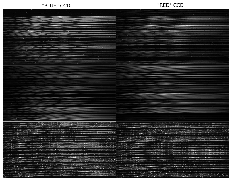
Figure 1.— Sample M2FS object (top), quartz flat (middle), and ThAr comparison spectrum (bottom) images from the “blue” (left) and “red” (right) CCDs used during the 47 Tuc observations. Up to 24 fibers per CCD (48 total) can be used with the M2FS setup employed here. Each set of 6 orders corresponds to one fiber. For the image orientations shown here, wavelength increases from left to right in each order. H$\alpha$ can be seen in all of the stellar object spectra. Note also the internal Littrow ghost reflections affecting several middle columns of each CCD. This affects a roughly 5–10 Å wide region in the reduced spectra of some orders and some fibers.

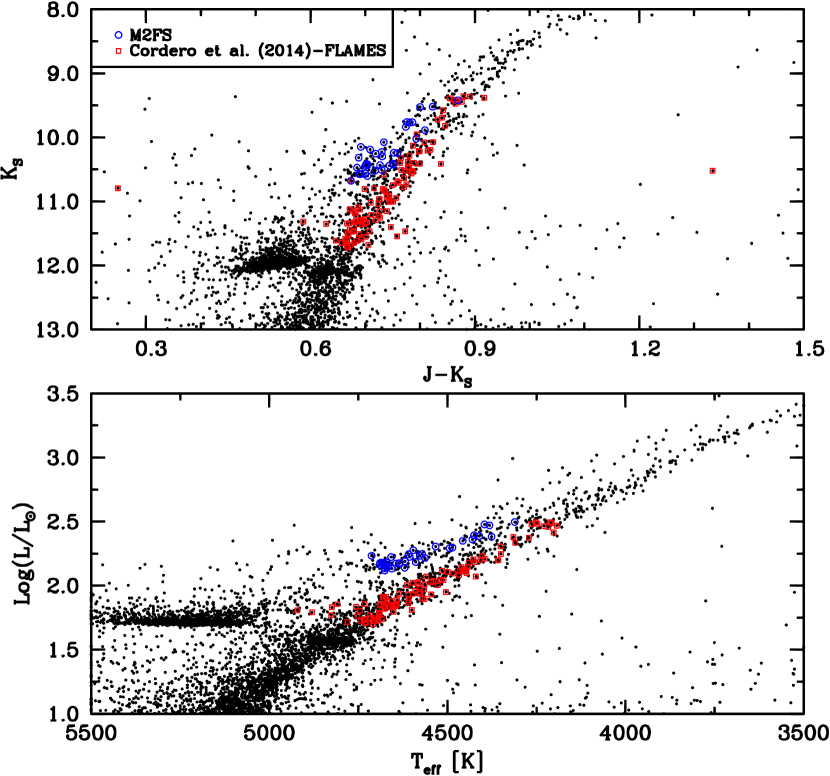
Figure 2.— top: Color–magnitude diagram illustrating the evolutionary state of AGB stars targeted in this work (open blue circles) and the complimentary RGB FLAMES–GIRAFFE data set (open red boxes) from Cordero et al. (2014). The filled black circles are from 2MASS (Skrutskie et al. 2006). bottom: A temperature–luminosity plot showing the selection of RGB and AGB stars from the McDonald et al. (2011) data.

2.2. Target Selection

The initial target selection and RGB/AGB separation was accomplished using the photometry, luminosity, and temperature values from McDonald et al. (2011). Since the data presented in Cordero et al. (2014) contained almost exclusively RGB stars, we selected only early AGB stars of comparable temperature from the McDonald et al. (2011) catalog for observation with M2FS. The data from McDonald et al. (2011) were matched to the Two Micron All–Sky Survey (2MASS; Skrutskie et al. 2006) database, and the 2MASS coordinates were used as input for the fiber plug plate configuration. Similarly, 2MASS coordinates and photometry were used to identify suitable guide, acquisition, and Shack–Hartmann stars required by the instrument. Although we obtained spectra of 42 AGB stars, 7 were discarded due to a failure to adequately converge to a stable solution of the model atmosphere parameters (see Section 3). A 2MASS color–magnitude diagram and temperature–luminosity plot for the final sample of 35 AGB stars, along with the comparative sample of 113 RGB stars from Cordero et al. (2014), are shown in Figure 2. The star identifications, coordinates, photometry, model atmosphere parameters, abundances, and heliocentric radial velocities for all 35 AGB stars are provided in Table 2.

Figure 3 compares the sky positions of the AGB and RGB 47 Tuc samples relative to the cluster center and half–light radius (r_h). We prioritized AGB stars residing within $\sim$1–2 r_h, but also sampled out to the same radial extent as the RGB data. The radial distribution of targets is relevant because one of the key science questions addressed in this paper is whether or not second generation RGB stars fail to evolve off the horizontal branch and ascend the AGB. There is growing evidence that while primordial (first generation) stars tend to follow the underlying cluster distribution at all radii, the intermediate and extreme stars (second generation) are often strongly concentrated near the cluster core (e.g., Carretta et al. 2010b; Kravtsov et al. 2010; Lardo et al. 2011; Johnson & Pilachowski 2012; Milone et al. 2012; Cordero et al. 2014; Li et al. 2014). Nataf et al. (2011) also find evidence that stars near the cluster core may be He enhanced (see also di Criscienzo et al. 2010). If He and Na are correlated then the most Na–rich AGB stars should reside near the core. Vesperini et al. (2013) note that the local ratio of second/first generation stars should match the global ratio at a half–mass radius of $\sim$1.5. Therefore, we expect that our AGB target selection will adequately sample the true AGB [Na/Fe] distribution and maximize our chances of finding Na–rich AGB stars, if they exist.

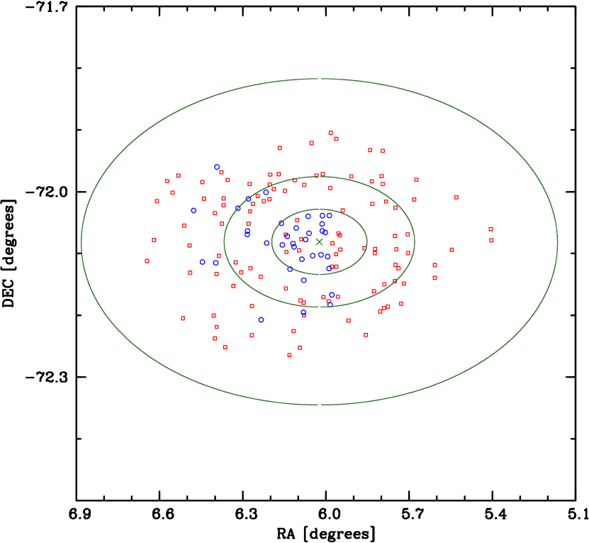
Figure 3.— Plot showing the sky coordinates of the AGB stars observed in this work (open blue circles) and the RGB FLAMES–GIRAFFE data (open red boxes) from Cordero et al. (2014). The green cross indicates the cluster center, and the outer ellipses designate 1, 2, and 5 times the half–light radius (3.17$\arcmin$; Harris 1996).

2.3. Data Reduction

The basic data reduction procedures, including bias correction and trimming the overscan regions, were carried out using the IRAF task ccdproc. Since each amplifier image on each CCD has a slightly different value for read noise and gain, the individual amplifier object and calibration files are reduced separately in a manner similar to that used for Hectochelle reductions (Caldwell et al. 2009; Szentgyorgyi et al. 2011). The individual bias corrected and trimmed exposures are then rotated, translated, and combined using the IRAF tasks imtranspose and imjoin to create one file per exposure (i.e., images such as those in Figure 1).

Although the M2FS setup used here produces 6 orders per fiber, the more advanced data reduction procedures should in principle be similar to the default setup in which each fiber produces a single order. Therefore, we used repeated calls of the IRAF task dohydra to handle aperture identification and tracing, scattered light removal, flat–field correction, ThAr wavelength calibration, cosmic–ray removal, and object spectrum extraction. We ran dohydra on all fibers of each CCD, but only extracted one order from each fiber per dohydra loop. Since the sky fibers are spread across both CCDs, we skipped the sky subtraction routine inside dohydra. Instead, we used scombine to create a master sky spectrum for each order of each exposure and subtracted this from the object spectra with the skysub routine.

Following sky subtraction, each order of every exposure was normalized with the continuum IRAF routine and then median combined with scombine to increase the S/N and remove any remaining cosmic–rays. The full wavelength range spanned by each order is listed in Table 1. However, as is evident in Figure 1, the S/N decreases near the edges of each order. Therefore, we removed the lower S/N regions of each order that had correspondingly higher S/N regions in an adjacent order. The final (“effective”) wavelength coverage of each order after carrying out this procedure is given in Table 1. We also chose to remove, rather than combine, overlapping regions between orders because there is a small difference in resolution between the bluer and redder orders. A sample M2FS spectrum with all orders merged is shown in Figure 4.

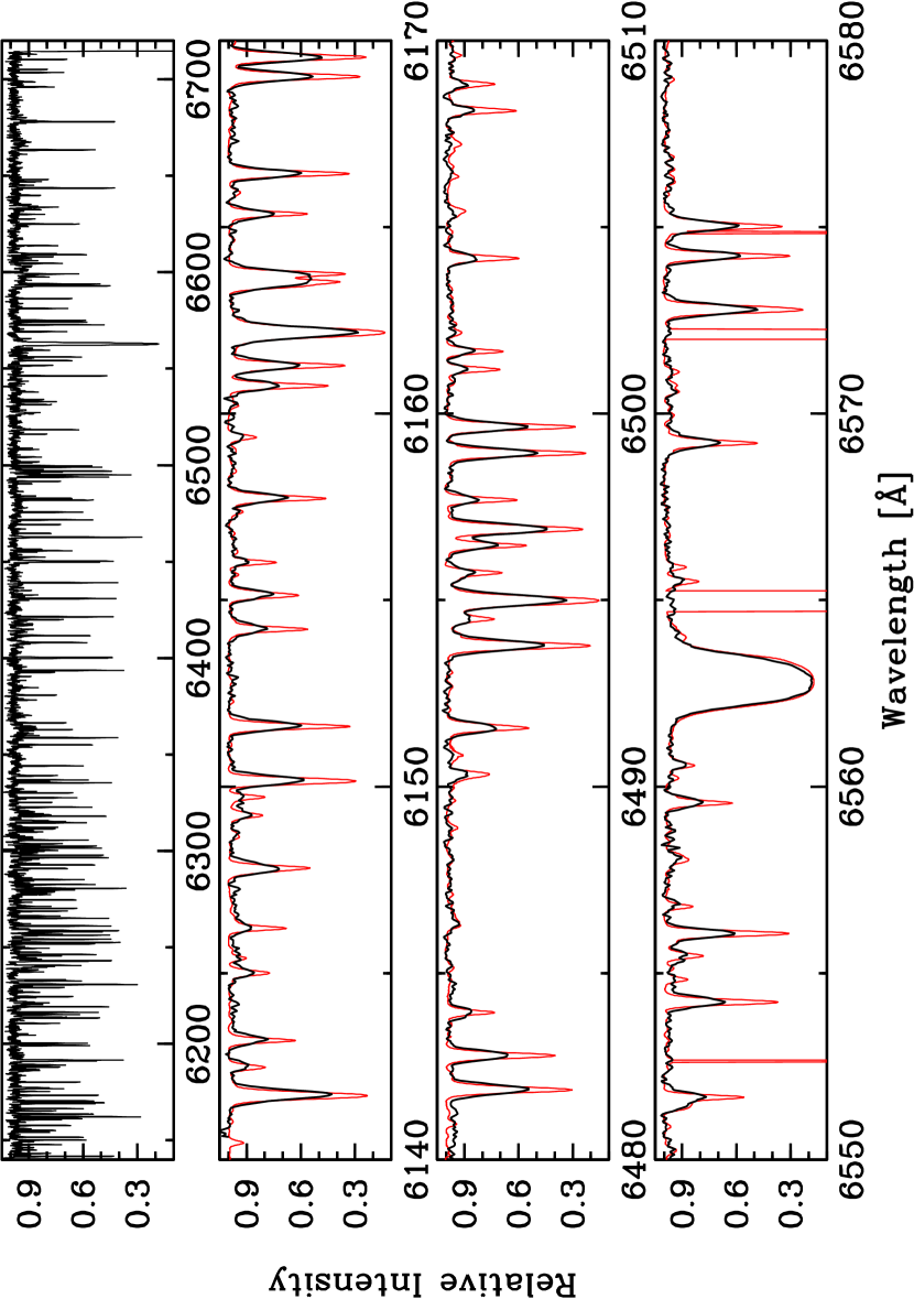
Figure 4.— Sample M2FS spectrum of a 47 Tuc AGB star after merging the orders. The top panel shows the full wavelength range. The lower panels show sample spectral regions, including the 6154/6160 Å Na I lines used to derive the Na abundances for this work. The higher resolution Arcturus atlas (Hinkle et al. 2000) is shown in red for comparison. Both stars have similar effective temperatures.

3. DATA ANALYSIS

3.1. Model Stellar Atmospheres

The model atmosphere parameters effective temperature (T_eff), surface gravity (log(g)), metallicity ([Fe/H]), and microturbulence (vt) were determined spectroscopically and in a manner identical to that used for the FLAMES–GIRAFFE sample of Cordero et al. (2014). Specifically, T_eff was determined by removing trends in log $\epsilon$(Fe I) as a function of excitation potential, log(g) was determined by enforcing ionization equilibrium with the Fe I and Fe II lines, and vt was determined by removing trends in log $\epsilon$(Fe I) as a function of line strength. We adopted a generic model atmosphere with T_eff=4600 K, log(g)=1.5 (cgs), [Fe/H]=–0.7, and vt=1.5 km s^-1 as the starting point and then iterated to simultaneously solve all four model atmosphere parameters. The average of the derived [Fe I/H] and [Fe II/H] abundances was used to update the model metallicity in each iteration. Opacity and atmosphere stratification discrepancies due to the difference between [Fe/H] and [M/H] were roughly accounted for by using the $\alpha$–enhanced ATLAS9 model atmospheres from Castelli & Kurucz (2004). We interpolated within the available ATLAS9 grid to obtain the final model atmospheres used in the abundance analysis. Since the range in both temperatures and luminosities spanned by the RGB and AGB samples is relatively small (see Figure 2), we have not adopted any corrections to either the model atmosphere parameters or abundance ratios due to departures either from plane parallel geometry or local thermodynamic equilibrium (LTE). However, Figure 5 shows that the spectroscopic temperatures are well correlated with temperatures estimates from (J–K_S)_o 2MASS photometry. Using the color–temperature relation given in González Hernández & Bonifacio (2009), we find an average difference between the spectroscopic and photometric temperatures of 14 K ($\sigma$=85 K). We found a similar result for the RGB FLAMES–GIRAFFE sample in Cordero et al. (2014), with an average difference of 28 K ($\sigma$=53 K).

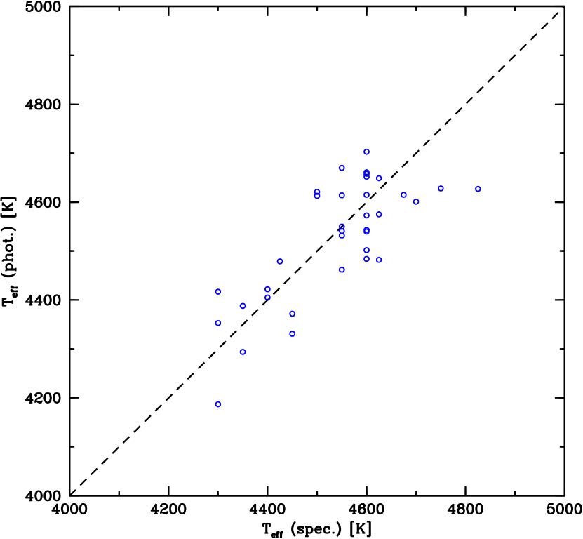
Figure 5.— Plot comparing the effective temperature values derived by enforcing excitation equilibrium (T_eff spec.) and using the J–K_S color–temperature relation from González Hernández & Bonifacio (2009; T_eff phot.). The dashed line indicates perfect agreement.

3.2. Iron Abundance Determinations

The line list used to determine Fe I and Fe II abundances was similar to that used by Cordero et al. (2014), but augmented to include additional lines available in the M2FS spectra. The [Fe/H] abundances, and also model atmosphere parameters, were based on equivalent width measurements for an average of 45 Fe I lines and 4 Fe II lines per star. The equivalent widths were measured manually using the semi–automated code developed for Johnson et al. (2014), which fits individual or blended Gaussian profiles and is aided by a simple machine learning algorithm. The final abundances were calculated using the abfind driver of the LTE line analysis code MOOG (Sneden 1973; 2010 version). We adopted the same solar abundance as Cordero et al. (2014) of log $\epsilon$(Fe)_⊙=7.52. The list of lines and atomic data used for this work is provided in Table 3, and the log(gf) values were redetermined using a high S/N day light sky spectrum taken with M2FS. For the lines in common between this work and Cordero et al. (2014), the average difference in adopted log(gf) values was zero for both Fe I ($\sigma$=0.09) and Fe II ($\sigma$=0.04).

The random measurement uncertainty estimated by $\sigma$/$\sqrt{N}$, where $\sigma$ is the line–to–line dispersion and N is the number of lines measured, is relatively small for both iron species. Specifically, the average random measurement uncertainty for log $\epsilon$(Fe I) is 0.02 and for log $\epsilon$(Fe II) is 0.04. The [Fe/H] error column listed in Table 2 represents the combined uncertainty for both Fe I and Fe II abundances. Additional uncertainty in the iron abundance determination comes from errors in the model atmosphere parameters. We estimate that the uncertainty in T_eff, log(g), [M/H], and vt, based solely on enforcing excitation equilibrium, ionization equilibrium, and removing trends in log $\epsilon$(Fe I) as a function of line strength, are: 50 K, 0.10 (cgs), 0.05 dex, and 0.10 km s^-1, respectively. The combined sensitivity of both [Fe I/H] and [Fe II/H] to these changes in model atmosphere parameters is 0.09 dex, on average.

As mentioned in Section 3.1, we did not apply any corrections to the [Fe I/H] and [Fe II/H] abundances for departures from LTE. However, Lapenna et al. (2014) used high resolution (R$\sim$48,000) spectra of 24 AGB and 11 RGB stars in 47 Tuc to derive [Fe I/H] and [Fe II/H] abundances and found that only in the RGB sample did the neutral and singly ionized abundances match. Lapenna et al. (2014) further conclude that for AGB stars Fe I lines should not be used to derive [Fe/H] abundances and that determining surface gravity from ionization equilibrium, which is the method used here, is also invalid for AGB stars. The strong difference in Fe I line formation due to departures from LTE in similar temperature AGB but not RGB stars is a puzzling result and does not match recent theoretical investigations (e.g., Bergemann et al. 2012; Lind et al. 2012). We note that Ivans et al. (2001) also encountered problems deriving model atmosphere parameters for evolved stars in the more metal–poor ([Fe/H]$\approx$–1.2) globular cluster M5, and also decided to set the [Fe/H] scale using only Fe II and photometric log(g) values.

For the lines analyzed in this work, the Bergemann et al. (2012) and Lind et al. (2012) calculations suggest departures from LTE should affect [Fe I/H] at about the 0.05 dex level in both RGB and AGB stars. In both populations the [Fe II/H] abundance is mostly unaffected because Fe II is the dominant ionization state. However, the difference in [Fe/H] abundances and model atmosphere parameters derived for RGB and AGB stars using ionization and excitation equilibrium is not expected to produce large systematic offsets when assuming LTE. In fact, after reconciling a small difference in temperature scale between our RGB and AGB samples (see Section 4), we do not find any significant difference in [Fe/H] for the two populations.

Finally, we note that Lapenna et al. (2014) and this work have four AGB stars in common. A comparison of the model atmosphere parameters, [Fe/H] abundances, and radial velocities is provided in Table 4. We find average differences in T_eff, log(g), [Fe I/H], [Fe II/H], vt, and RV_helio. of 50 K, –0.12 (cgs), $+$0.12 dex, $+$0.05 dex, –0.09 km s^-1, and –0.11 km s^-1, respectively. The surface gravity differences are even smaller if the most highly discrepant star (2M00235852–7206177) is removed. The [Fe I/H] values from Lapenna et al. (2014) are the most discrepant abundances; however, we derive similar [Fe II/H] abundances (within the stated uncertainties) to Lapenna et al. (2014) while simultaneously solving for the model atmosphere parameters via spectroscopic methods and obtaining identical [Fe I/H] and [Fe II/H] ratios. The conflicting observational claims between this work and Lapenna et al. (2014) suggest that a better understanding of RGB and AGB atmospheres is needed before ionization equilibrium is fully dismissed as a viable method for determining [Fe/H] and surface gravity in AGB (but not RGB) stars. However, we cannot rule out that the failure of 7 AGB stars in our sample (17$\%$) to converge to a stable spectroscopic solution is related to the discrepancies found by Lapenna et al. (2014) and Ivans et al. (2001).

3.3. Sodium Abundance Determinations

For consistency with the Cordero et al. (2014) [Na/Fe] data, we measured sodium abundances using the same line list (see also Table 3 for a summary of the transition parameters for the Na I lines), the synth driver in MOOG, and adopted log $\epsilon$(Na)_⊙=6.33. The dominant molecular contaminator near the 6154/6160 Å Na I lines in the temperature and metallicity regime analyzed here is CN. While we did not have individual C, N, and O abundances for the target stars, the local CN features were fit assuming that the stars were well–mixed (e.g., [C/Fe]=–0.5; [O/Fe]=$+$0.1; ¹²C/¹³C=4); the nitrogen abundance was varied as a free parameter. The CN line list was adopted from the Kurucz (1994) database (but see also a recent update by Sneden et al. 2014). A sample spectrum synthesis for a typical M2FS spectrum is shown in Figure 6. The final [Na/Fe] values given in Table 2 do not include any corrections for departures from LTE in the analysis. However, the log $\epsilon$(Na) non–LTE corrections are $\lesssim$0.10 dex in an absolute sense (e.g., Lind et al. 2011; Thygesen et al. 2014), and the differential non–LTE corrections for [Na/Fe] due to surface gravity differences between AGB and RGB stars is typically $<$0.05 dex.

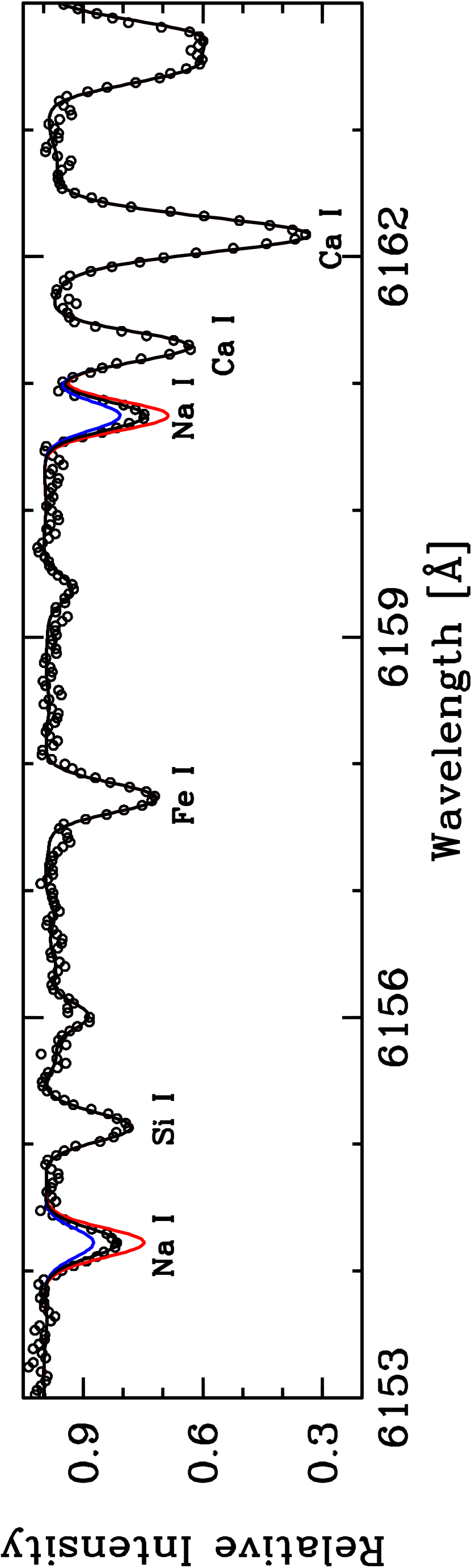
Figure 6.— Sample Na I spectrum synthesis for a typical 47 Tuc AGB star. The black line is the best fit synthesis and the red/blue lines are the best fit Na abundance changed by $\pm$0.3 dex.

The random measurement errors for log $\epsilon$(Na I) are only slightly larger than for $\epsilon$(Fe I), with an average of 0.03 dex. This value reflects the difference in sodium abundance between the 6154 and 6160 Å Na I lines. The [Na/Fe] error column of Table 2 takes into account both the measurement uncertainty in [Fe/H] and [Na/H]. As with iron, additional sources of uncertainty are due to errors in the derived model atmosphere parameters. Using the same estimates as in Section 3.2, the average uncertainty from model atmosphere parameters alone in the [Na/Fe] ratio is 0.05 dex.

4. BASIC RESULTS

Although recent color–magnitude diagrams of 47 Tuc suggest the cluster has a complex star formation history (Anderson et al. 2009; di Criscienzo et al. 2010; Nataf et al. 2011; Milone et al. 2012; Monelli et al. 2013; Li et al. 2014), there is no evidence supporting a substantial spread in [Fe/H]. Instead, literature work suggests the cluster has an average [Fe/H]$\approx$–0.60 to –0.80, with a star–to–star dispersion $\lesssim$0.10 dex (e.g., Carretta & Gratton 1997; Alves–Brito et al. 2005; Wylie et al. 2006; Koch & McWilliam 2008; Carretta et al. 2009; Gratton et al. 2013; Cordero et al. 2014; Dobrovolskas et al. 2014; Thygesen et al. 2014). In agreement with past work, we find an average [Fe/H]=–0.68 and a star–to–star dispersion of $\sigma$=0.08. This result is similar to, but more metal–rich than, the RGB FLAMES–GIRAFFE sample of Cordero et al. (2014) that found $\langle$[Fe/H]$\rangle$=–0.75 ($\sigma$=0.10). The 0.07 dex difference in [Fe/H] between the AGB and RGB samples is possibly tied to a systematic offset in the temperature scales between the two data sets. A comparison of the spectroscopically determined T_eff values with those derived from photometric spectral energy distribution fitting in McDonald et al. (2011) finds systematic offsets of –20 K ($\sigma$=74 K) for the RGB sample and $+$35 K ($\sigma$=71 K) for the AGB sample. If the [Fe/H] abundances are redetermined using temperatures (and corresponding gravities) that are 35 K lower and 20 K higher for the AGB and RGB stars, respectively, then the AGB [Fe/H] values decrease by 0.05 dex and the RGB [Fe/H] values increase by 0.02 dex. This brings both data sets into agreement at $\langle$[Fe/H]$\rangle$=–0.73.

In contrast to [Fe/H], 47 Tuc exhibits a significant spread in [Na/Fe] abundance. For the AGB stars analyzed here, [Na/Fe] ranges from –0.11 to $+$0.62 with $\langle$[Na/Fe]$\rangle$=$+$0.21 ($\sigma$=0.17). The large dispersion in [Na/Fe] is typical for globular clusters (e.g., see reviews by Kraft 1994; Gratton et al. 2004; 2012), and the large fraction of stars with [Na/Fe]$>$0 matches previous observations of 47 Tuc RGB, horizontal branch, and main–sequence turn–off stars (e.g., Carretta et al. 2004; Alves–Brito et al. 2005; Koch & McWilliam 2008; Carretta et al. 2009; D’Orazi et al. 2010; Worley & Cottrell 2012; Gratton et al. 2013; Cordero et al. 2014; Dobrovolskas et al. 2014; Thygesen et al. 2014). The possible temperature scale difference between the AGB and RGB samples also affects sodium. However, the change in [Na/Fe] is only an increase of 0.02 dex for the AGB stars and a decrease of 0.01 dex for the RGB stars. A more detailed comparison between the AGB and RGB [Na/Fe] abundances is provided in Section 5.

Radial velocities were also measured for each star in order to verify cluster membership. We used the cross–correlation code XCSAO (Kurtz & Mink 1998), and the heliocentric correction was determined using the IRAF task rvcorrect. The velocities were determined relative to a synthetic rest frame spectrum with T_eff=4600 K, log(g)=1.5 (cgs), [Fe/H]=–0.70, and vt=1.5 km s^-1, and the XCSAO routine was only run on order 55 (see Table 1) of a single exposure for each star. Order 55 was selected because it exhibits several strong lines but does not contain many problematic features (e.g., telluric bands; unusually strong or broad lines). The average measurement uncertainty returned by XCSAO for the radial velocities was 0.18 km s^-1. We find an average heliocentric radial velocity of –18.56 km s^-1 ($\sigma$=10.21 km s^-1). The average cluster velocity determined here is in good agreement with past work, which ranges from –16.86 km s^-1 to –22.43 km s^-1 (Dinescu et al. 1999; Carretta et al. 2004; Alves–Brito et al. 2005; Carretta et al. 2009; Dobrovolskas et al. 2014; Lapenna et al. 2014). All of the stars observed with M2FS have velocities consistent with cluster membership.

5. INTERPRETING THE AGB AND RGB [NA/FE] DISTRIBUTIONS

Recent work mentioned in Section 1 suggests that AGB and RGB stars in some globular clusters may show distinctly different chemical compositions. In particular, the AGB populations are suspected of having systematically lower ratios of second generation (CN–strong; Na–enhanced; He–enhanced) to first generation (CN–weak; Na–poor; He–normal) stars, compared to the RGB populations. Evidence linking the minimum mass and blue extension of stars along the horizontal branch to the AGB/RGB star count ratio (Gratton et al. 2010) indicates that the apparent composition difference between AGB and RGB stars is likely due to some RGB stars not evolving through the AGB phase, rather than an in situ process altering the envelope composition of some stars before or after the horizontal branch phase. The apparent loss of Na–rich second generation stars between the RGB and AGB is most evident in the metal–poor blue horizontal branch cluster NGC 6752, which has a Na–poor/Na–rich ratio of 30:70 on the RGB and a 100:0 ratio on the AGB (Campbell et al. 2013). Furthermore, Sandquist & Bolte (2004) note that NGC 6752 exhibits a low ratio of AGB to horizontal branch stars, and interpret this observation as an indication that some fraction of RGB stars fail to evolve through the AGB phase.

Since the number of dedicated studies comparing RGB and AGB abundance patterns is still small (e.g., see Campbell et al. 2006; their Table 1), evidence is insufficient to determine whether the peculiar lack of Na–rich AGB stars in NGC 6752 is more the exception or the rule. Therefore, the data provided here offer insight into a possible counter example. 47 Tuc is approximately 10$\times$ more massive than NGC 6752 (e.g., Pryor & Meylan 1993), 7$\times$ more metal–rich, contains almost exclusively red horizontal branch stars (e.g., Lee et al. 1994; see also Figure 2), and has a high AGB/RGB ratio (Gratton et al. 2010). In the left panels of Figure 7, we compare the [Na/Fe] abundances between the AGB and RGB samples in 47 Tuc as a function of T_eff, as a binned distribution, and as a cumulative distribution. The AGB [Na/Fe] distribution appears to be shifted to lower values than the RGB population, and also has fewer stars with [Na/Fe]$>$$+$0.4 but more with [Na/Fe]$<$$+$0.1. After correcting for the AGB/RGB temperature scale differences, comparing only the average values yields $\langle$[Na/Fe]$\rangle$=$+$0.23 for the AGB sample and $\langle$[Na/Fe]$\rangle$=$+$0.35 for the RGB FLAMES–GIRAFFE sample. Similarly, the ratio of Na–poor to Na–rich stars is 63:37 for the AGB sample and 45:55 for the RGB sample. The 0.12 dex average [Na/Fe] abundance difference between AGB and RGB stars in 47 Tuc is similar to, though less extreme than, the 0.34 dex average difference found by Campbell et al. (2013) for NGC 6752 (see also the right panels of Figure 7).

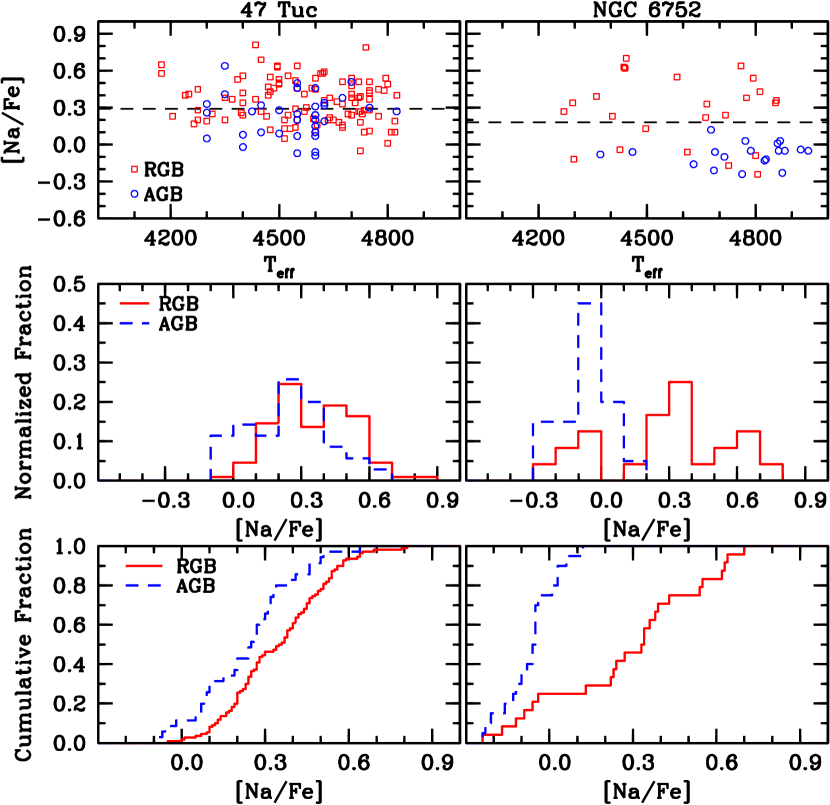
Figure 7.— Plots of [Na/Fe] versus T_eff (top), [Na/Fe] histograms using 0.1 dex bins (middle), and cumulative distribution functions (bottom) are shown for 47 Tuc (left) and NGC 6752 (right). While the 47 Tuc AGB data are from this work, the 47 Tuc RGB data are from the FLAMES–GIRAFFE sample in Cordero et al. (2014) and the RGB/AGB data for NGC 6752 are from Campbell et al. (2013). The dashed horizontal lines in the top panels separate the Na–poor and Na–rich populations, based on the inflection point in the cumulative distribution panels. Typical measurement errors for [Na/Fe] are $\sim$0.1 dex. Note that for 47 Tuc the AGB [Na/Fe] abundances have been increased by 0.02 dex and the RGB abundances, including the Na–poor/Na–rich separation, decreased by 0.01 dex, in order to bring the two samples onto a common temperature scale (see also Section 4).

However, an examination of the dispersion ($\sigma$) and interquartile range (IQR) values of the AGB and RGB stars in 47 Tuc, which are mostly insensitive to systematic reduction or analysis differences between data sets, reveals that the two populations are similar. Specifically, the 47 Tuc AGB stars have $\sigma$_AGB=0.17 and IQR_AGB=0.23 and the RGB stars have $\sigma$_RGB=0.18 and IQR_RGB=0.27. These values strongly contrast with the results of NGC 6752 in which the AGB has $\sigma$_AGB=0.09 and IQR_AGB=0.10 and the RGB has $\sigma$_RGB=0.28 and IQR_RGB=0.37. The stark contrast in AGB/RGB [Na/Fe] dispersion and IQR distributions between the two clusters suggests that only a small fraction ($<$20$\%$) of Na–rich RGB stars in 47 Tuc fail to evolve through at least the early AGB phase, instead of the 100$\%$ fraction observed in NGC 6752.

Color–magnitude diagram analyses also support the notion that both Na–poor and Na–rich RGB stars evolve through the horizontal branch and early AGB phases in 47 Tuc. Aside from previous spectroscopic detections of both CN–strong (Na–rich) and CN–weak (Na–poor) stars on 47 Tuc’s AGB (e.g., Mallia 1978; Briley 1997), we note that Monelli et al. (2013) make use of the (U–B)–(B–I) color index, which is correlated with [Na/Fe], and find a bimodal AGB color spread. These data indicate that at least two stellar populations, containing roughly equal proportions but with different light element chemistry, are present along 47 Tuc’s AGB. Furthermore, color–magnitude diagrams do not show a significant population of blue horizontal branch stars that may fail to ascend the AGB (e.g., Anderson et al. 2009; Bergbusch & Stetson 2009; Dieball et al. 2009; Milone et al. 2012), and stars spanning the entire RGB [Na/Fe] range are found on the red horizontal branch (Gratton et al. 2013). This contrasts with the color–magnitude diagram of NGC 6752, which shows a significant population of blue and extreme horizontal branch stars (e.g., Grundahl et al. 1999), and also is known to contain AGB–manqué stars (e.g., Momany et al. 2002). However, the horizontal branch differences between 47 Tuc and NGC 6752 are largely driven by metallicity, as is qualitatively illustrated in the isochrone tracks of Figure 8.

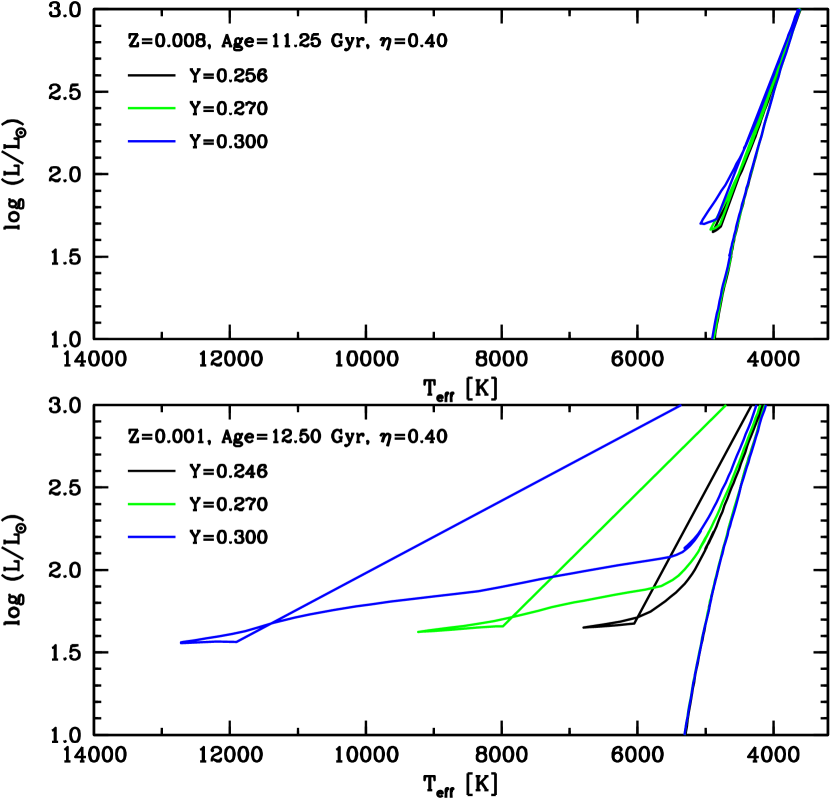
Figure 8.— top: Stellar isochrones from Bertelli et al. (2008) are shown assuming the age and metallicity of 47 Tuc from VandenBerg et al. (2013). The black (Y=0.256), green (Y=0.270), and blue (Y=0.300) isochrones illustrate how the horizontal branch changes as a function of He abundance. A Reimers (1975) mass loss constant ($\eta$) of 0.4 is assumed for all cases. bottom: A similar plot assuming the age and metallicity of NGC 6752.

Since it is clear from Figure 7 that the RGB and AGB [Na/Fe] distributions are significantly different in absolute abundance and dispersion between 47 Tuc and NGC 6752, the question remains as to what ties together RGB composition and post–RGB evolution. As mentioned previously, a commonly adopted solution is that Na–rich stars have a higher He abundance, and that the lower masses of He–rich/Na–rich horizontal branch stars prevent them from evolving through the AGB phase. At least for the extreme case of NGC 6752, Charbonnel et al. (2013) note that stars with masses less than about 0.735 M_⊙ and Y$\gtrsim$0.31 do not ascend the AGB. However, the required He–enhancements are significantly larger than those estimated from photometry ($\Delta$Y$\sim$0.03–0.04; Milone et al. 2013), but Charbonnel et al. (2013) further suggest the maximum photometric He spread could be underestimated. For 47 Tuc, the He spread is estimated to be even smaller ($\Delta$Y$\lesssim$0.02–0.03; e.g., di Criscienzo et al. 2010; Nataf et al. 2011; Milone et al. 2012) than in NGC 6752, and as Figure 8 shows even RGB stars with Y=0.3 are still likely to ascend the AGB at 47 Tuc’s metallicity (e.g., see also Valcarce et al. 2012 and references therein). Despite having significantly different metallicities and horizontal branch morphologies, the AGB/RGB composition difference in 47 Tuc may be more analagous to the case of M13 where Johnson & Pilachowski (2012) found that only the most Na–rich and O–poor stars (presumably also the most He–rich stars) failed to reach the AGB. We note that the paucity of O–poor stars on M13’s AGB, albeit from a sample of only $\sim$10 AGB stars, is observed despite the failure (so far) of investigators to find a strongly He–enhanced population (Sandquist et al. 2010; Smith et al. 2014). Could a different parameter be driving the AGB/RGB composition disparity?

Campbell et al. (2013) proposed that, in addition to He enhancement for the Na–rich stars, a substantial ad hoc increase in the mass loss rate (20$\times$ the RGB value) for NGC 6752 stars on the blue horizontal branch may be required to prevent further evolution up the AGB. However, Cassisi et al. (2014) note that the required mass loss rate of $\sim$10^-9 M_⊙ year^-1 is several orders of magnitude higher than those allowed by current analyses of hot horizontal branch and B subdwarf stars. Additionally, horizontal branch simulations by Cassisi et al. (2014) that accurately reproduce the R₂ parameter (N_AGB/N_HB) for NGC 6752, M3, and M13, but do not invoke enhanced mass loss, also predict that $\sim$50$\%$ of NGC 6752’s AGB stars should be Na–rich (albeit with lower Y than the most extreme values). These results indicate that enhanced mass loss for a particular subset of horizontal branch stars is unlikely to be the key link between RGB composition and post–RGB evolution. Furthermore, even if processes associated with the radiative levitation of metals in blue horizontal branch stars played a role in mass loss and/or the subsequent envelope composition of AGB stars, 47 Tuc lacks a significant population of horizontal branch stars with T_eff$\gtrsim$11,000 K that would experience this effect (e.g., Behr et al. 2003).

6. CONCLUSIONS

The data presented here indicate that the average [Na/Fe] abundance of AGB stars in the Galactic globular cluster 47 Tuc is 0.12 dex lower than that of the RGB stars. Additionally, the ratio of Na–poor to Na–rich AGB stars is 63:37 compared to 45:55 for the RGB stars. However, both populations exhibit a similar dispersion and IQR of [Na/Fe]. This result strongly contrasts with that found by Campbell et al. (2013) in the globular cluster NGC 6752 where the AGB consists of only Na–poor stars with a small star–to–star [Na/Fe] dispersion. The 47 Tuc [Na/Fe] distribution suggests that $\lesssim$20$\%$ of Na–rich RGB stars fail to reach the early AGB, which is similar to the case of M13 where only the most Na–rich and O–poor stars are missing from the AGB. For 47 Tuc, the cluster’s relatively high metallicity leads to a predominantly red horizontal branch morphology, and no significant population of hot horizontal branch and AGB–manqué stars, which likely make up the missing Na–rich component of NGC 6752’s (and M13’s) AGB, has been found. Unlike the case for NGC 6752, however, in 47 Tuc it seems that at least some Na–rich RGB stars evolve through the early AGB phase. We conclude that RGB [Na/Fe] abundances alone are not a unique predictor of future AGB evolution in all clusters.

Several remaining questions must be addressed before a definitive link between stellar composition, cluster horizontal branch morphology, and AGB evolution can be formed. For example, if He abundance, in addition to metallicity and age, is a significant factor in defining a globular cluster’s horizontal branch morphology and a star’s post–RGB evolution, why do the $\Delta$Y values estimated from photometry appear too low in a cluster such as NGC 6752 to prevent Na–rich stars from ascending the AGB? Are the He–enhancements actually underestimated, as was suggested by Charbonnel et al. (2013)? What roles do additional parameters such as mass loss, He core rotation, CNO abundance, and/or environment play in defining a star’s horizontal branch and eventual AGB evolution? What separates clusters such as 47 Tuc and M13, which lose only a fraction of Na–rich stars before the AGB, to those such as NGC 6752, which lose 100$\%$? A deeper understanding of the critical parameters controlling horizontal branch and AGB evolution, along with additional studies comparing large samples of RGB and AGB chemical compositions, seems required in order to fully place the failure (or not) of some Na–rich stars to ascend the AGB into context with the developing narrative of forming multiple populations in globular clusters.

Table 1M2FS Bulge_GC1 Filter Orders

Order	Full Range	Effective Range
	(Å)	(Å)
58	6122$-$6205	6138$-$6190
57	6152$-$6315	6190$-$6310
56	6262$-$6426	6310$-$6410
55	6376$-$6543	6410$-$6525
54	6494$-$6664	6525$-$6650
53	6617$-$6721	6650$-$6720

Note. — Note that orders 58 and 53 are only partially covered due to the filter response cut–off.

Table 2Basic Data and Results

Star ID	RA (J2000)	DEC (J2000)	J	H	KS	Teff	log(g)	[Fe/H]	[Fe/H] Error	vt	[Na/Fe]	[Na/Fe] Error	RVhelio.	RVhelio. Error
2MASS	(degrees)	(degrees)	(mag.)	(mag.)	(mag.)	(K)	(cgs)			(km s-1)			(km s-1)	(km s-1)
2M00235484$-$7210009	5.978539	$-$72.166939	11.266	10.697	10.575	4600	1.71	$-$0.72	0.05	1.70	$+$0.18	0.05	$-$5.47	0.14
2M00235632$-$7210590	5.984693	$-$72.183060	11.114	10.514	10.412	4500	1.60	$-$0.71	0.06	1.70	$+$0.26	0.08	$-$19.66	0.18
2M00235701$-$7202185	5.987543	$-$72.038475	11.145	10.593	10.445	4825	2.18	$-$0.57	0.04	1.95	$+$0.25	0.05	$-$6.03	0.19
2M00235728$-$7207274	5.988676	$-$72.124290	10.610	9.948	9.836	4400	1.47	$-$0.69	0.03	1.65	$+$0.06	0.07	$-$3.12	0.14
2M00235852$-$7206177	5.993859	$-$72.104919	11.005	10.436	10.317	4600	1.33	$-$0.78	0.02	1.75	$+$0.44	0.03	$-$1.03	0.14
2M00240062$-$7203573	6.002621	$-$72.065926	10.343	9.625	9.520	4350	1.17	$-$0.76	0.03	1.75	$+$0.39	0.08	$-$26.60	0.18
2M00240304$-$7202193	6.012702	$-$72.038712	10.840	10.284	10.148	4625	1.93	$-$0.72	0.02	1.75	$+$0.17	0.06	$-$28.23	0.20
2M00240310$-$7203482	6.012947	$-$72.063393	11.139	10.578	10.435	4600	1.92	$-$0.66	0.07	1.60	$+$0.08	0.07	$-$9.69	0.15
2M00240330$-$7203075	6.013772	$-$72.052101	11.139	10.578	10.435	4550	1.67	$-$0.76	0.06	1.95	$+$0.48	0.06	$-$12.31	0.15
2M00240427$-$7206074	6.017792	$-$72.102081	10.814	10.124	10.021	4450	1.73	$-$0.68	0.06	1.40	$+$0.08	0.06	$-$24.41	0.16
2M00241142$-$7206126	6.047624	$-$72.103516	11.184	10.559	10.440	4600	1.72	$-$0.72	0.03	1.55	$+$0.05	0.03	$-$20.35	0.14
2M00241462$-$7204018	6.060919	$-$72.067184	11.161	10.568	10.410	4600	1.85	$-$0.65	0.05	1.60	$+$0.22	0.06	$-$23.14	0.18
2M00241531$-$7202231	6.063815	$-$72.039757	10.552	9.886	9.771	4400	1.42	$-$0.58	0.03	1.60	$-$0.04	0.04	$-$13.49	0.13
2M00241755$-$7204385	6.073161	$-$72.077370	11.351	10.733	10.677	4600	2.11	$-$0.59	0.05	0.90	$-$0.08	0.06	$-$33.09	0.19
2M00241912$-$7208360	6.079687	$-$72.143356	10.992	10.395	10.240	4425	1.13	$-$0.82	0.06	1.55	$+$0.25	0.06	$-$31.87	0.17
2M00241945$-$7211426	6.081072	$-$72.195183	11.262	10.646	10.562	4750	2.03	$-$0.56	0.05	1.70	$+$0.28	0.05	$-$17.19	0.14
2M00242074$-$7206332	6.086458	$-$72.109245	11.157	10.615	10.472	4550	1.27	$-$0.75	0.03	1.45	$+$0.05	0.03	$-$22.51	0.15
2M00242572$-$7203307	6.107181	$-$72.058540	10.696	10.017	9.887	4450	1.15	$-$0.68	0.05	1.70	$+$0.30	0.05	$-$11.54	0.15
2M00242763$-$7205213	6.115141	$-$72.089264	11.004	10.428	10.245	4550	1.64	$-$0.67	0.08	1.70	$+$0.18	0.09	$-$20.96	0.16
2M00242846$-$7205019	6.118608	$-$72.083862	11.176	10.581	10.425	4625	1.65	$-$0.76	0.03	1.75	$+$0.32	0.05	$-$22.21	0.17
2M00243106$-$7207311	6.129429	$-$72.125313	10.898	10.280	10.189	4700	1.90	$-$0.61	0.04	1.70	$+$0.49	0.05	$-$24.35	0.15
2M00243337$-$7204200	6.139076	$-$72.072243	10.973	10.362	10.254	4600	1.95	$-$0.61	0.06	1.60	$+$0.29	0.07	$+$2.90	0.13
2M00243771$-$7205100	6.157149	$-$72.086121	10.324	9.651	9.524	4300	1.20	$-$0.71	0.10	1.75	$+$0.31	0.10	$-$38.05	0.22
2M00243851$-$7203038	6.160488	$-$72.051079	10.958	10.304	10.228	4550	1.48	$-$0.70	0.03	1.65	$+$0.23	0.04	$-$22.80	0.17
2M00245127$-$7204588	6.213660	$-$72.083000	11.161	10.543	10.434	4550	1.50	$-$0.68	0.05	1.60	$+$0.44	0.06	$-$19.99	0.17
2M00245189$-$7200031	6.216213	$-$72.000862	11.237	10.639	10.519	4625	1.63	$-$0.70	0.04	1.65	$+$0.30	0.06	$-$30.43	0.23
2M00245600$-$7212266	6.233351	$-$72.207397	11.125	10.510	10.421	4675	2.15	$-$0.64	0.06	1.40	$+$0.36	0.07	$+$0.69	0.21
2M00250716$-$7200415	6.279846	$-$72.011536	10.537	9.865	9.761	4300	1.37	$-$0.66	0.03	1.65	$+$0.03	0.03	$-$17.09	0.13
2M00250791$-$7203490	6.282998	$-$72.063629	11.264	10.658	10.575	4600	1.52	$-$0.76	0.06	1.70	$+$0.13	0.07	$-$33.36	0.16
2M00250809$-$7204092	6.283737	$-$72.069244	11.027	10.408	10.296	4600	1.69	$-$0.59	0.06	1.65	$+$0.22	0.06	$-$23.45	0.17
2M00251614$-$7201359	6.317278	$-$72.026649	10.809	10.187	10.075	4550	1.43	$-$0.56	0.05	1.75	$-$0.09	0.11	$-$12.04	0.13
2M00253428$-$7157352	6.392834	$-$71.959793	10.549	9.896	9.763	4350	1.08	$-$0.79	0.03	1.75	$+$0.62	0.04	$-$18.29	0.15
2M00253529$-$7206543	6.397057	$-$72.115105	11.308	10.727	10.604	4500	1.38	$-$0.84	0.06	1.40	$+$0.07	0.06	$-$17.45	0.19
2M00254689$-$7206494	6.445395	$-$72.113731	11.238	10.646	10.508	4600	2.01	$-$0.57	0.08	1.70	$-$0.11	0.08	$-$13.47	0.18
2M00255446$-$7201491	6.476949	$-$72.030312	10.289	9.558	9.420	4300	1.27	$-$0.55	0.08	1.75	$+$0.24	0.12	$-$29.39	0.57

Table 3Line List

Wavelength	Ion	E.P.	log(gf)
(Å)		(eV)
6154.23	11.0	2.101	$-$1.57
6160.75	11.0	2.103	$-$1.27
6145.41	26.0	3.368	$-$3.58
6148.65	26.0	4.320	$-$2.63
6151.62	26.0	2.176	$-$3.31
6157.73	26.0	4.076	$-$1.19
6159.37	26.0	4.607	$-$1.88
6165.36	26.0	4.143	$-$1.54
6173.33	26.0	2.223	$-$2.89
6180.20	26.0	2.727	$-$2.71
6187.99	26.0	3.943	$-$1.75
6213.43	26.0	2.223	$-$2.52
6219.28	26.0	2.198	$-$2.33
6220.78	26.0	3.881	$-$2.39
6226.73	26.0	3.883	$-$2.12
6229.23	26.0	2.845	$-$2.93
6232.64	26.0	3.654	$-$1.24
6240.65	26.0	2.223	$-$3.32
6252.56	26.0	2.404	$-$1.63
6253.83	26.0	4.733	$-$1.53
6270.22	26.0	2.858	$-$2.62
6271.28	26.0	3.332	$-$2.76
6322.69	26.0	2.588	$-$2.31
6335.33	26.0	2.198	$-$2.11
6336.82	26.0	3.686	$-$0.59
6358.70	26.0	0.859	$-$4.32
6362.88	26.0	4.186	$-$2.03
6380.74	26.0	4.186	$-$1.35
6385.72	26.0	4.733	$-$1.87
6392.54	26.0	2.279	$-$3.95
6393.60	26.0	2.433	$-$1.48
6408.02	26.0	3.686	$-$0.91
6411.65	26.0	3.654	$-$0.40
6430.85	26.0	2.176	$-$1.89
6469.19	26.0	4.835	$-$0.80
6472.15	26.0	4.371	$-$2.89
6475.62	26.0	2.559	$-$2.88
6481.87	26.0	2.279	$-$2.92
6483.94	26.0	1.485	$-$5.30
6494.98	26.0	2.404	$-$1.15
6495.74	26.0	4.835	$-$1.02
6496.47	26.0	4.795	$-$0.56
6498.94	26.0	0.958	$-$4.61
6509.62	26.0	4.076	$-$2.88
6518.37	26.0	2.831	$-$2.58
6533.93	26.0	4.558	$-$1.29
6546.24	26.0	2.758	$-$1.71
6551.68	26.0	0.990	$-$5.73
6556.79	26.0	4.796	$-$1.61
6569.21	26.0	4.733	$-$0.21
6581.21	26.0	1.485	$-$4.73
6591.31	26.0	4.593	$-$1.98
6592.91	26.0	2.727	$-$1.51
6593.87	26.0	2.433	$-$2.25
6597.56	26.0	4.795	$-$0.98
6609.11	26.0	2.559	$-$2.58
6609.68	26.0	0.990	$-$5.78
6633.41	26.0	4.835	$-$1.26
6633.75	26.0	4.558	$-$0.71
6634.11	26.0	4.795	$-$1.23
6648.08	26.0	1.011	$-$5.79
6665.43	26.0	1.557	$-$5.60
6710.32	26.0	1.485	$-$4.81
6713.74	26.0	4.795	$-$1.43
6715.38	26.0	4.607	$-$1.54
6716.24	26.0	4.580	$-$1.81
6149.26	26.1	3.889	$-$2.66
6247.56	26.1	3.892	$-$2.33
6369.46	26.1	2.891	$-$4.09
6385.45	26.1	5.553	$-$2.63
6432.68	26.1	2.891	$-$3.63
6456.38	26.1	3.903	$-$2.03
6482.20	26.1	6.219	$-$1.67
6516.08	26.1	2.891	$-$3.33

Table 4AGB stars in common with Lapenna et al. (2014)

Star Name	Teffspec.	log(g)spec.	[Fe I/H]	[Fe II/H]	vt	RVhelio.	Star Name	Teffphot.	log(g)phot.	[Fe I/H]	[Fe II/H]	vt	RVhelio.
Ours	(K)	(cgs)			km s-1	km s-1	L2014	(K)	(cgs)			km s-1	km s-1
2M00235852$-$7206177	4600	1.33	$-$0.78	$-$0.78	1.75	$-$1.03	100119	4500	1.65	$-$0.85	$-$0.71	1.80	$-$0.83
2M00241142$-$7206126	4600	1.72	$-$0.72	$-$0.72	1.55	$-$20.75	100142	4550	1.70	$-$0.90	$-$0.80	1.60	$-$20.41
2M00242763$-$7205213	4550	1.64	$-$0.67	$-$0.67	1.70	$-$20.96	200021	4550	1.70	$-$0.83	$-$0.84	1.90	$-$21.07
2M00242846$-$7205019	4625	1.65	$-$0.76	$-$0.76	1.75	$-$22.21	200023	4575	1.75	$-$0.81	$-$0.79	1.80	$-$22.19

References

- Alves-Brito et al. (2005) Alves-Brito, A., Barbuy, B., Ortolani, S., et al. 2005, A&A, 435, 657
- Anderson et al. (2009) Anderson, J., Piotto, G., King, I. R., Bedin, L. R., & Guhathakurta, P. 2009, ApJ, 697, L58
- Bastian et al. (2013) Bastian, N., Lamers, H. J. G. L. M., de Mink, S. E., et al. 2013, MNRAS, 436, 2398
- Bekki (2011) Bekki, K. 2011, MNRAS, 412, 2241
- Behr (2003) Behr, B. B. 2003, ApJS, 149, 67
- Bergbusch & Stetson (2009) Bergbusch, P. A., & Stetson, P. B. 2009, AJ, 138, 1455
- Bergemann et al. (2012) Bergemann, M., Lind, K., Collet, R., Magic, Z., & Asplund, M. 2012, MNRAS, 427, 27
- Bertelli et al. (2008) Bertelli, G., Girardi, L., Marigo, P., & Nasi, E. 2008, A&A, 484, 815
- Boehm-Vitense (1979) Böhm-Vitense, E. 1979, ApJ, 234, 521
- Bragaglia et al. (2010) Bragaglia, A., Carretta, E., Gratton, R. G., et al. 2010, ApJ, 720, L41
- Briley et al. (1996) Briley, M. M., Smith, V. V., Suntzeff, N. B., et al. 1996, Nature, 383, 604
- Briley (1997) Briley, M. M. 1997, AJ, 114, 1051
- Briley et al. (2004) Briley, M. M., Harbeck, D., Smith, G. H., & Grebel, E. K. 2004, AJ, 127, 1588
- Burgh et al. (2007) Burgh, E. B., Bershady, M. A., Westfall, K. B., & Nordsieck, K. H. 2007, PASP, 119, 1069
- Caldwell et al. (2009) Caldwell, N., Harding, P., Morrison, H., et al. 2009, AJ, 137, 94
- Campbell et al. (2006) Campbell, S. W., Lattanzio, J. C., & Elliott, L. M. 2006, Mem. Soc. Astron. Italiana, 77, 864
- Campbell et al. (2010) Campbell, S. W., Yong, D., Wylie-de Boer, E. C., et al. 2010, Mem. Soc. Astron. Italiana, 81, 1004
- Campbell et al. (2012) Campbell, S. W., Yong, D., Wylie-de Boer, E. C., et al. 2012, ApJ, 761, L2
- Campbell et al. (2013) Campbell, S. W., D’Orazi, V., Yong, D., et al. 2013, Nature, 498, 198
- Carretta & Gratton (1997) Carretta, E., & Gratton, R. G. 1997, A&AS, 121, 95
- Carretta et al. (2004) Carretta, E., Gratton, R. G., Bragaglia, A., Bonifacio, P., & Pasquini, L. 2004, A&A, 416, 925
- Carretta et al. (2009) Carretta, E., Bragaglia, A., Gratton, R. G., et al. 2009, A&A, 505, 117
- Carretta et al. (2010) Carretta, E., Bragaglia, A., Gratton, R. G., et al. 2010a, A&A, 516, A55
- Carretta et al. (2010) Carretta, E., Bragaglia, A., D’Orazi, V., Lucatello, S., & Gratton, R. G. 2010b, A&A, 519, A71
- Carretta et al. (2011) Carretta, E., Bragaglia, A., Gratton, R., D’Orazi, V., & Lucatello, S. 2011, A&A, 535, A121
- Cassisi et al. (2014) Cassisi, S., Salaris, M., Pietrinferni, A., Vink, J. S., & Monelli, M. 2014, arXiv:1410.3599
- Castellani et al. (2006) Castellani, V., Iannicola, G., Bono, G., et al. 2006, A&A, 446, 569
- Castelli & Kurucz (2004) Castelli, F., & Kurucz, R. L. 2004, arXiv:astro-ph/0405087
- Charbonnel et al. (2013) Charbonnel, C., Chantereau, W., Decressin, T., Meynet, G., & Schaerer, D. 2013, A&A, 557, L17
- Cohen & Meléndez (2005) Cohen, J. G., & Meléndez, J. 2005, AJ, 129, 303
- Conroy & Spergel (2011) Conroy, C., & Spergel, D. N. 2011, ApJ, 726, 36
- Cordero et al. (2014) Cordero, M. J., Pilachowski, C. A., Johnson, C. I., et al. 2014, ApJ, 780, 94
- D’Antona & Ventura (2007) D’Antona, F., & Ventura, P. 2007, MNRAS, 379, 1431
- D’Ercole et al. (2008) D’Ercole, A., Vesperini, E., D’Antona, F., McMillan, S. L. W., & Recchi, S. 2008, MNRAS, 391, 825
- D’Orazi et al. (2010) D’Orazi, V., Lucatello, S., Gratton, R., et al. 2010, ApJ, 713, L1
- di Criscienzo et al. (2010) di Criscienzo, M., Ventura, P., D’Antona, F., Milone, A., & Piotto, G. 2010, MNRAS, 408, 999
- de Mink et al. (2009) de Mink, S. E., Pols, O. R., Langer, N., & Izzard, R. G. 2009, A&A, 507, L1
- Decressin et al. (2007) Decressin, T., Meynet, G., Charbonnel, C., Prantzos, N., & Ekström, S. 2007a, A&A, 464, 1029
- Decressin et al. (2007) Decressin, T., Charbonnel, C., & Meynet, G. 2007b, A&A, 475, 859
- Denisenkov & Denisenkova (1990) Denisenkov, P. A., & Denisenkova, S. N. 1990, Soviet Astronomy Letters, 16, 275
- Denissenkov & VandenBerg (2003) Denissenkov, P. A., & VandenBerg, D. A. 2003, ApJ, 593, 509
- Denissenkov & Hartwick (2014) Denissenkov, P. A., & Hartwick, F. D. A. 2014, MNRAS, 437, L21
- Dinescu et al. (1999) Dinescu, D. I., Girard, T. M., & van Altena, W. F. 1999, AJ, 117, 1792
- Dobrovolskas et al. (2014) Dobrovolskas, V., Kučinskas, A., Bonifacio, P., et al. 2014, A&A, 565, A121
- Dupree et al. (2011) Dupree, A. K., Strader, J., & Smith, G. H. 2011, ApJ, 728, 155
- González Hernández & Bonifacio (2009) González Hernández, J. I., & Bonifacio, P. 2009, A&A, 497, 497
- Gratton et al. (2001) Gratton, R. G., Bonifacio, P., Bragaglia, A., et al. 2001, A&A, 369, 87
- Gratton et al. (2004) Gratton, R., Sneden, C., & Carretta, E. 2004, ARA&A, 42, 385
- Gratton et al. (2010) Gratton, R. G., D’Orazi, V., Bragaglia, A., Carretta, E., & Lucatello, S. 2010, A&A, 522, A77
- Gratton et al. (2012) Gratton, R. G., Carretta, E., & Bragaglia, A. 2012, A&A Rev., 20, 50
- Gratton et al. (2013) Gratton, R. G., Lucatello, S., Sollima, A., et al. 2013, A&A, 549, AA41
- Greggio & Renzini (1990) Greggio, L., & Renzini, A. 1990, ApJ, 364, 35
- Grundahl et al. (1999) Grundahl, F., Catelan, M., Landsman, W. B., Stetson, P. B., & Andersen, M. I. 1999, ApJ, 524, 242
- Harris (1996) Harris, W. E. 1996, AJ, 112, 1487
- Hinkle et al. (2000) Hinkle, K., Wallace, L., Valenti, J., & Harmer, D. 2000, Visible and Near Infrared Atlas of the Arcturus Spectrum 3727-9300 A ed. Kenneth Hinkle, Lloyd Wallace, Jeff Valenti, and Dianne Harmer. (San Francisco: ASP) ISBN: 1-58381-037-4, 2000
- Ivans et al. (1999) Ivans, I. I., Sneden, C., Kraft, R. P., et al. 1999, AJ, 118, 1273
- Ivans et al. (2001) Ivans, I. I., Kraft, R. P., Sneden, C., et al. 2001, AJ, 122, 1438
- Johnson & Pilachowski (2012) Johnson, C. I., & Pilachowski, C. A. 2012, ApJ, 754, L38
- Johnson et al. (2014) Johnson, C. I., Rich, R. M., Kobayashi, C., Kunder, A., & Koch, A. 2014, AJ, 148, 67
- Karakas et al. (2006) Karakas, A. I., Fenner, Y., Sills, A., Campbell, S. W., & Lattanzio, J. C. 2006, ApJ, 652, 1240
- Koch & McWilliam (2008) Koch, A., & McWilliam, A. 2008, AJ, 135, 1551
- Kraft (1994) Kraft, R. P. 1994, PASP, 106, 553
- Kravtsov et al. (2010) Kravtsov, V., Alcaíno, G., Marconi, G., & Alvarado, F. 2010, A&A, 512, L6
- Kurtz & Mink (1998) Kurtz, M. J., & Mink, D. J. 1998, PASP, 110, 934
- Kurucz (1994) Kurucz, R. L. 1994, Atomic Data for Opacity Calculations, Kurucz CD-ROM No. 1
- Langer et al. (1993) Langer, G. E., Hoffman, R., & Sneden, C. 1993, PASP, 105, 301
- Lapenna et al. (2014) Lapenna, E., Mucciarelli, A., Lanzoni, B., et al. 2014, arXiv:1410.3841
- Lardo et al. (2011) Lardo, C., Bellazzini, M., Pancino, E., et al. 2011, A&A, 525, A114
- Lee et al. (1994) Lee, Y.-W., Demarque, P., & Zinn, R. 1994, ApJ, 423, 248
- Li et al. (2014) Li, C., de Grijs, R., Deng, L., et al. 2014, ApJ, 790, 35
- Lind et al. (2011) Lind, K., Asplund, M., Barklem, P. S., & Belyaev, A. K. 2011, A&A, 528, A103
- Lind et al. (2012) Lind, K., Bergemann, M., & Asplund, M. 2012, MNRAS, 427, 50
- Mallia (1978) Mallia, E. A. 1978, A&A, 70, 115
- Marino et al. (2014) Marino, A. F., Milone, A. P., Przybilla, N., et al. 2014, MNRAS, 437, 1609
- Mateo et al. (2012) Mateo, M., Bailey, J. I., Crane, J., et al. 2012, Proc. SPIE, 8446, 4
- McDonald et al. (2011) McDonald, I., Boyer, M. L., van Loon, J. T., et al. 2011, ApJS, 193, 23
- Milone et al. (2012) Milone, A. P., Piotto, G., Bedin, L. R., et al. 2012, ApJ, 744, 58
- Milone et al. (2013) Milone, A. P., Marino, A. F., Piotto, G., et al. 2013, ApJ, 767, 120
- Momany et al. (2002) Momany, Y., Piotto, G., Recio-Blanco, A., et al. 2002, ApJ, 576, L65
- Monelli et al. (2013) Monelli, M., Milone, A. P., Stetson, P. B., et al. 2013, MNRAS, 431, 2126
- Mucciarelli et al. (2014) Mucciarelli, A., Lovisi, L., Lanzoni, B., & Ferraro, F. R. 2014, ApJ, 786, 14
- Nataf et al. (2011) Nataf, D. M., Gould, A., Pinsonneault, M. H., & Stetson, P. B. 2011, ApJ, 736, 94
- Norris et al. (1981) Norris, J., Cottrell, P. L., Freeman, K. C., & Da Costa, G. S. 1981, ApJ, 244, 205
- Pasquini et al. (2011) Pasquini, L., Mauas, P., Käufl, H. U., & Cacciari, C. 2011, A&A, 531, A35
- Pilachowski et al. (1996) Pilachowski, C. A., Sneden, C., Kraft, R. P., & Langer, G. E. 1996, AJ, 112, 545
- Piotto et al. (2007) Piotto, G., Bedin, L. R., Anderson, J., et al. 2007, ApJ, 661, L53
- Piotto (2009) Piotto, G. 2009, IAU Symposium, 258, 233
- Prantzos et al. (2007) Prantzos, N., Charbonnel, C., & Iliadis, C. 2007, A&A, 470, 179
- Pryor & Meylan (1993) Pryor, C., & Meylan, G. 1993, Structure and Dynamics of Globular Clusters, 50, 357
- Ramírez & Cohen (2002) Ramírez, S. V., & Cohen, J. G. 2002, AJ, 123, 3277
- Ramírez & Cohen (2003) Ramírez, S. V., & Cohen, J. G. 2003, AJ, 125, 224
- Reimers (1975) Reimers, D. 1975, Memoires of the Societe Royale des Sciences de Liege, 8, 369
- Renzini (2008) Renzini, A. 2008, MNRAS, 391, 354
- Sandquist & Bolte (2004) Sandquist, E. L., & Bolte, M. 2004, ApJ, 611, 323
- Skrutskie et al. (2006) Skrutskie, M. F., Cutri, R. M., Stiening, R., et al. 2006, AJ, 131, 1163
- Smith & Norris (1993) Smith, G. H., & Norris, J. E. 1993, AJ, 105, 173
- Smith et al. (2014) Smith, G. H., Dupree, A. K., & Strader, J. 2014, PASP, 126, 901
- Smolinski et al. (2011) Smolinski, J. P., Martell, S. L., Beers, T. C., & Lee, Y. S. 2011, AJ, 142, 126
- Sneden (1973) Sneden, C. 1973, ApJ, 184, 839
- Sneden et al. (2000) Sneden, C., Ivans, I. I., & Kraft, R. P. 2000, Mem. Soc. Astron. Italiana, 71, 657
- Sneden et al. (2014) Sneden, C., Lucatello, S., Ram, R. S., Brooke, J. S. A., & Bernath, P. 2014, ApJS, 214, 26
- Suntzeff (1981) Suntzeff, N. B. 1981, ApJS, 47, 1
- Szentgyorgyi et al. (2011) Szentgyorgyi, A., Furesz, G., Cheimets, P., et al. 2011, PASP, 123, 1188
- Thygesen et al. (2014) Thygesen, A. O., Sbordone, L., Andrievsky, S., et al. 2014, arXiv:1409.4694
- Valcarce & Catelan (2011) Valcarce, A. A. R., & Catelan, M. 2011, A&A, 533, A120
- Valcarce et al. (2012) Valcarce, A. A. R., Catelan, M., & Sweigart, A. V. 2012, A&A, 547, A5
- VandenBerg et al. (2013) VandenBerg, D. A., Brogaard, K., Leaman, R., & Casagrande, L. 2013, ApJ, 775, 134
- Ventura & D’Antona (2009) Ventura, P., & D’Antona, F. 2009, A&A, 499, 835
- Ventura et al. (2009) Ventura, P., Caloi, V., D’Antona, F., et al. 2009, MNRAS, 399, 934
- Vesperini et al. (2013) Vesperini, E., McMillan, S. L. W., D’Antona, F., & D’Ercole, A. 2013, MNRAS, 429, 1913
- Worley & Cottrell (2012) Worley, C. C., & Cottrell, P. L. 2012, PASA, 29, 29
- Wylie et al. (2006) Wylie, E. C., Cottrell, P. L., Sneden, C. A., & Lattanzio, J. C. 2006, ApJ, 649, 248
- Yong et al. (2009) Yong, D., Grundahl, F., D’Antona, F., et al. 2009, ApJ, 695, L62
- Yong et al. (2014) Yong, D., Grundahl, F., & Norris, J. E. 2014, arXiv:1411.1474