TTP14-034

Radiative generation of neutrino mixing: degenerate masses and threshold corrections

Wolfgang Gregor Hollik

Institut für Theoretische Teilchenphysik, Karlsruhe Institute of Technology

Engesserstraße 7, D-76131 Karlsruhe, Germany

Degenerate neutrino masses are excluded by experiment. The experimentally measured mass squared differences together with the yet undetermined absolute neutrino mass scale allow for a quasi-degenerate mass spectrum. For the lightest neutrino mass larger than roughly $0.1\,\mathrm{eV}$, we analyze the influence of threshold corrections at the electroweak scale. We show that typical one-loop corrections can generate the observed neutrino mixing as well as the mass differences starting from exactly degenerate masses at the tree-level. Those threshold corrections have to be explicitly flavor violating. Flavor diagonal, non-universal corrections are not sufficient to simultaneously generate the correct mixing and the mass differences. We apply the new insights to an extension of the Minimal Supersymmetric Standard Model with non-minimal flavor violation in the soft breaking terms and discuss the low-energy threshold corrections to the light neutrino mass matrix in that model.

PACS: 14.60.Pq, 12.60.Jv

1 Introduction

A direct measurement of neutrino masses is still missing. The perspective of data from tritium decay in the near future probes the effective electron neutrino mass down to $0.2\,\mathrm{eV}$ [1]. Complementary to direct searches are constraints from cosmology [2, 3] where the tightest bound on the sum of (active) neutrino masses released by the Planck collaboration is under certain assumptions $\sum m_{\nu}<0.23\,\mathrm{eV}$ [4]. Including galaxy clustering and lensing data in addition to the standard observation from the cosmic microwave background and baryon acoustic oscillations, this bound turns into an observation in a “degenerate active neutrino scenario”, $\sum m_{\nu}=(0.320\pm 0.081)\,\mathrm{eV}$ [5]. The reported sum of neutrino masses shows a significant deviation of about $3.2\,\sigma$ from the minimal value $\sum m_{\nu}=0.059\,\mathrm{eV}$ which is allowed by a massless lightest neutrino and the differences of mass squares:

$$\Delta m_{21}^{2} =7.50^{+0.19}_{-0.17}\times 10^{-5}\,\mathrm{eV}^{2},$$ (1.1)

$$\Delta m_{31}^{2} =2.457\pm 0.047\times 10^{-3}\,\mathrm{eV}^{2},$$

where $\Delta m_{ji}^{2}=m_{j}^{2}-m_{i}^{2}$ and we restricted ourselves to the result of a normal hierarchy ($\Delta m_{31}^{2}>0$) as follows from a global fit of neutrino oscillation data [6].

The cosmological bounds as stated above disfavor a possible direct detection of a neutrino mass from tritium decay. In any case, presuming such a discovery (which would be around $m_{\nu_{e}}=0.35\,\mathrm{eV}$ or higher) or taking the cosmological observation $\sum m_{\nu}=0.32\,\mathrm{eV}$ for granted, we observe a neutrino mass spectrum that is (quasi-)degenerate. In the first case, the three neutrino masses differ only about one percent. The second scenario has at least the third mass about ten percent larger than the lightest and second-lightest.

The three neutrino mass eigenvalues are calculated, once the absolute scale $m_{0}$ is fixed (we focus on a normal mass hierarchy):

$$\left|m_{1}\right|=m_{0}\,,\qquad\qquad\left|m_{2}\right|=\sqrt{m_{0}^{2}+\Delta m_{21}^{2}}\,,\qquad\qquad\left|m_{3}\right|=\sqrt{m_{0}^{2}+\Delta m_{31}^{2}}.$$

Now we see, that $m_{1\ldots 3}$ are basically the same numbers, in the limit $m_{0}^{2}\gg\Delta m^{2}$. The striking feature of such a quasi-degenerate mass spectrum is, that the small deviations from exact degeneracy can be seen as a small perturbation originating in quantum corrections to neutrino masses.

It is well-known, that for degenerate neutrinos quantum corrections are important [7, 8, 9, 10, 11, 12, 13, 14, 15, 16, 17, 18, 19]. However, the question is, whether the stringent Planck bounds still allow for dominant contributions from quantum corrections. We shall focus on the influence of low-energy threshold corrections as they may arise in several extensions of the Standard Model around the $\mathrm{TeV}$ scale. The importance of threshold corrections in the MSSM was already pointed out [11, 13, 14, 15, 18], we apply them to the current phenomenology of neutrino masses and mixing (simultaneously accommodating a non-zero third mixing angle and still being consistent with the mass bound).

Furthermore, those loop corrections to neutrino masses may also lead to the desired mixing pattern as will be shown. The observed values for the three mixing angles are taken from the same global fit that determines the $\Delta m^{2}$ [6]

$$\sin^{2}\theta_{12} =0.304\pm 0.012,$$ (1.2)

$$\sin^{2}\theta_{13} =0.0219^{+0.0010}_{-0.0011},$$

$$\sin^{2}\theta_{23} =0.451\pm 0.001,$$

where we follow the standard parametrization of any three-dimensional rotation matrix that can be seen as three successive rotations and the Dirac $\mathrm{CP}$ phase $\delta_{\mathrm{CP}}$ associated to the 1-3-rotation

$$\boldsymbol{U}(\theta_{12},\theta_{13},\theta_{23},\delta_{\mathrm{CP}},\alpha_{1},\alpha_{2}) =\;\boldsymbol{U}_{23}(\theta_{23})\;\boldsymbol{U}_{13}(\theta_{13},\delta_{\mathrm{CP}})\;\boldsymbol{U}_{12}(\theta_{12})\;\boldsymbol{P}(\alpha_{1},\alpha_{2})$$ (1.3)

$$=\begin{pmatrix}c_{12}c_{13}&s_{12}c_{13}&s_{13}e^{-\mathrm{i}\,\delta_{\mathrm{CP}}}\\ -s_{12}c_{23}-c_{12}s_{23}s_{13}e^{\mathrm{i}\,\delta_{\mathrm{CP}}}&c_{12}c_{23}-s_{12}s_{23}e^{\mathrm{i}\,\delta_{\mathrm{CP}}}s_{13}&s_{23}c_{13}\\ s_{12}s_{23}-c_{12}c_{23}s_{13}e^{\mathrm{i}\,\delta_{\mathrm{CP}}}&-c_{12}s_{23}-s_{12}c_{23}s_{13}e^{\mathrm{i}\,\delta_{\mathrm{CP}}}&c_{23}c_{13}\end{pmatrix}\;\boldsymbol{P},$$

where $s_{ij}=\sin\theta_{ij}$ and $c_{ij}=\cos\theta_{ij}$ and the angles $\theta_{ij}$ parametrize the rotation in the $i$-$j$ plane. The phase matrix $\boldsymbol{P}=\operatorname{diag}(e^{\mathrm{i}\,\alpha_{1}},e^{\mathrm{i}\,\alpha_{2}},1)$ contains the Majorana phases which are absent in the case of Dirac neutrinos.

We work in a basis, where the charged lepton Yukawa couplings are diagonal and generate the small neutrino masses via a seesaw-inspired model [20, 21, 22, 23, 24, 25, 26] that leads to a nonrenormalizable operator suppressed by a reasonably heavy scale $M$ [27]:

$$\mathcal{L}^{\ell}_{\mathrm{Y}}\supset Y^{\mathrm{e}}_{\alpha}L_{\alpha}\cdot H\;e_{\alpha}+\frac{h^{\alpha\beta}}{M}(L_{\alpha}\cdot H)(L_{\beta}\cdot H)+\;\text{h.\,c.\ },$$ (1.4)

where $H$ denotes the SM Higgs doublet whose neutral component acquires a vev and $L_{\alpha}$ is the lepton doublet of flavor $\alpha=\mathrm{e},\muup,\tauup$: $L_{\alpha}=(\nu_{\mathrm{L},\alpha},\ell_{\mathrm{L},\alpha})$ of left-handed fields and $e_{\alpha}$ denotes the right-handed charged leptons. If the couplings $h^{\alpha\beta}$ are $\mathcal{O}(1)$ couplings, the mass of the light neutrinos scales as $v^{2}/M$. To end up with $m_{\nuup}\lesssim 1\,\mathrm{eV}$, the scale $M$ has to be $\mathcal{O}(10^{14}\,\mathrm{GeV})$.

We therefore explicitly work with Majorana neutrinos, which is manifest in a symmetric neutrino mass matrix, $h^{\alpha\beta}=h^{\beta\alpha}$, and the Majorana phase matrix $\boldsymbol{P}$ of Eq. (1.3). Since the charged lepton masses are diagonal, $\boldsymbol{U}$ of Eq. (1.3) diagonalizes the neutrino mass matrix and shows up as mixing matrix in the weak charged current interaction which is known as Pontecorvo-Maki-Nakagawa-Sakata (PMNS) matrix [28, 29].

A Majorana mass term does not allow to rotate away complex phases into redefinitions of the fields. Majorana neutrino masses are in general complex and the two Majorana phases $\alpha_{1},\alpha_{2}$ can be absorbed in a redefinition of the masses:

$$\bar{\boldsymbol{m}}^{\nu}=\boldsymbol{U}^{\text{T}}\boldsymbol{m}^{\nu}\boldsymbol{U}=\operatorname{diag}(|m_{1}|e^{-2\mathrm{i}\,\alpha_{1}},|m_{2}|e^{-2\mathrm{i}\,\alpha_{2}},m_{3}),$$ (1.5)

where $\boldsymbol{U}$ is the mixing matrix of Eq. (1.3) without the phase matrix $\boldsymbol{P}$. Without loss of generality $m_{3}$ can be chosen real and positive. Under $\mathrm{CP}$ conservation, the choice $\alpha_{1,2}=0,\pm\frac{\pi}{2}$ results in the possibility of having two different signs for the masses $m_{1,2}$ reflecting different $\mathrm{CP}$ parities. In the following, we want to discuss the two scenarios where all three neutrinos have the same $\mathrm{CP}$ parity and where one has a different sign.

This paper is organized as follows: in the second section we discuss possible patterns of degenerate masses as was done in the literature some time ago. In earlier works, people focused on bi-maximal (or tri-bimaximal) tree-level mixing and considered deviations from that pattern, especially with only very small $\theta_{13}$. Nowadays, since $\theta_{13}$ is measured quite well, it is intriguing to re-examine exemplarily simple patterns in the threshold corrections and see whether they can deal with both rather large 1-3 mixing and the established mass square differences. In the same section we also consider the case with trivial mixing at tree-level and generate the mixing fully radiatively. We estimate the size of the threshold corrections needed to generate the observed mixing pattern. The same procedure also fits the masses. Furthermore, in Section 3 we give an explicit example of a supersymmetric model with exactly degenerate tree-level masses, in which threshold corrections generate the observed pattern of mass differences and mixings.

2 The influence of Quantum corrections

In general, quantum corrections to neutrino masses change the alignment pattern of mass eigenstates and mixing angles. A tree-level mass matrix $\boldsymbol{m}^{(0)}_{\nu}$ provides a special mixing pattern by misalignment of interaction (flavor) and mass eigenstates. This can be result of some flavor symmetry acting at the tree-level Lagrangian. Quantum corrections are, however, mixing different flavor eigenstates differently from the tree-level pattern, where the corrected mass matrix can be parametrized as

$$m^{\nuup}_{\alpha\beta}=m^{(0)}_{\alpha\beta}+m^{(0)}_{\alpha\gamma}I_{\gamma\beta}+I_{\alpha\gamma}m^{(0)}_{\gamma\beta},$$ (2.1)

and $I_{\alpha\beta}$ denote the corrections [11, 13, 14, 15]. Greek indices ($\alpha,\beta,\gamma=\mathrm{e},\muup,\tauup$) live in the interaction basis. Note, that the tree-level mass matrix $\boldsymbol{m}^{(0)}$ as well as the corrections $\boldsymbol{I}$ are symmetric in the case of Majorana neutrinos which is explicitly assumed by the use of the effective operator of Eq. (1.4). The physical mass matrix is then understood to be $\boldsymbol{m}^{\nuup}$. In general, quantum corrections are to be decomposed in contributions from the renormalization group (RG) and low-energy threshold corrections at the electroweak scale: $\boldsymbol{I}=\boldsymbol{I}^{\mathrm{RG}}+\boldsymbol{I}^{\mathrm{TH}}$.

The contributions from the renormalization group are known to give a sizable effect for quasi-degenerate neutrino masses [30, 31, 7, 8, 9, 32, 33]. Especially the choice of the same $\mathrm{CP}$ parity for two masses may lead to large mixing at low scale irrespective of the original mixing at the high scale [12], known as infrared fixed points [33]. The effect from the renormalization group severely depends on the Majorana phases: for a vanishing Majorana phase, maximal mixing patterns get diluted on the way to the high scale [10] for quasi-degenerate ($m_{0}\sim\mathcal{O}(1\,\mathrm{eV})$) neutrino masses. If the phase on the contrary is large or the overall mass scale much smaller than $1\,\mathrm{eV}$, maximal mixing is preserved. Likewise, zero mixing (as follows from the assignment $m_{1}=m_{2}=m_{3}$) is conserved [34] irrespective of the Majorana phase difference $|\alpha_{1}-\alpha_{2}|$. We therefore safely neglect those kinds of contributions that preserve specific mixing patterns anyway.

The main contribution to the mass splitting from the RG evolution is from the $\tauup$ Yukawa coupling and can be estimated to be $I^{\text{RG}}_{\tauup}\lesssim\frac{y_{\tauup}^{2}}{16\pi^{2}}\log\left(\frac{M}{M_{Z}}\right)$, where $M$ is the heavy scale of Eq. (1.4). In the cosmological allowed scenarios ($m_{0}\lesssim 0.1\,\mathrm{eV}$), the maximal splitting for large values of $\tan\beta$ in the MSSM and a heavy scale $M\leq 10^{14}\;\mathrm{GeV}$ is generically too small to generate the required splitting between $m_{3}$ and $m_{1,2}$ which has to be around $0.01\,\mathrm{eV}$, whereas $I_{\tauup}^{\text{RG}}\approx 4.6\times 10^{-3}$ with $\tan\beta=50$ and $M=10^{14}\,\mathrm{GeV}$. This correction, which is independent from the tree-level neutrino mass spectrum, still gives a sizable effect for $m_{0}=0\,\mathrm{eV}$ of about $10\%$ of the mass splitting $\sqrt{\Delta m_{31}^{2}}$. To keep $I_{\tauup}^{\text{RG}}$ even smaller, one either has to reduce $M$ or $\tan\beta$ or both. It is, however, interesting to verify whether low-energy threshold corrections themselves can account for the required mass splittings. Since for the degenerate spectrum $m_{1}^{(0)}=m_{2}^{(0)}=m_{3}^{(0)}$ zero mixing is preserved, the existence of a RG induced mass splitting due to the $\tau$ Yukawa coupling does not alter the qualitative discussion on that scenario below. This feature may be used to generate a larger $\Delta m_{31}^{2}$ compared to $\Delta m_{21}^{2}$ if the the threefold degeneracy is to be abandoned without the need of too large $I_{33}$.

Our main purpose is to analyze the pure threshold effects as they may arise from new physics around the electroweak scale (therefore we also neglect the running of neutrino parameters from the electroweak to the scale of interest). As we will see, threshold corrections to the neutrino mass matrix can be sufficient to generate the large observed mixings even if there is no specific mixing at the tree-level.

The tree-level mass matrix of Eq. (2.1) can be transformed into the mass eigenbasis using the tree-level mixing matrix $\boldsymbol{U}^{(0)}$:

$$m^{\nuup}_{ij}=m^{(0)}_{i}\delta_{ij}+\left(m^{(0)}_{i}+m^{(0)}_{j}\right)I_{ij},$$ (2.2)

where Latin indices $i,j$ are meant to be in the mass basis and $I_{ij}=\sum_{\alpha\beta}I_{\alpha\beta}U^{(0)}_{\alpha i}U^{(0)}_{\beta j}$.

In the case of exact degeneracy, $m_{1}^{(0)}=m_{2}^{(0)}=m_{3}^{(0)}$, the tree-level mixing is trivial, whereas it gets non-trivial if the masses have different $\mathrm{CP}$ parities (e.g. $m_{1}^{(0)}=-m_{2}^{(0)}=m_{3}^{(0)}$) or $\mathrm{CP}$ violation occurs [35, 36]. Including ($\mathrm{CP}$ conserving) threshold corrections, it is possible to lift the degeneracy [13, 15] without referring to $\mathrm{CP}$ phases [37]. We address the question whether low-energy threshold corrections have the power to generate significant deviations from a given tree-level mixing with one vanishing mixing angle or even generate the observed neutrino mixing fully radiatively in the trivial scenario. Note that for the $m_{1}^{(0)}=-m_{2}^{(0)}=m_{3}^{(0)}$ case, there is a free rotation in the 1-3 plane left where two mixing angles are determined from the tree-level flavor structure.

The $m_{1}^{(0)}=-m_{2}^{(0)}=m_{3}^{(0)}$ scenario

The assignment of different $\mathrm{CP}$ eigenvalues to different masses simplifies the situation of Eq. (2.2) tremendously:

$$\boldsymbol{m}^{\nuup}=m\begin{pmatrix}1+2U_{\alpha 1}U_{\beta 1}I_{\alpha\beta}&0&2U_{\alpha 1}U_{\beta 3}I_{\alpha\beta}\\ 0&-1-2U_{\alpha 2}U_{\beta 2}I_{\alpha\beta}&0\\ 2U_{\alpha 1}U_{\beta 3}I_{\alpha\beta}&0&1+2U_{\alpha 3}U_{\beta 3}I_{\alpha\beta}\end{pmatrix},$$ (2.3)

where summation over repeated indices is understood. The diagonalization of the 1-3 block can be done by requiring

$$\sum_{\alpha\beta}U_{\alpha 1}U_{\beta 3}I_{\alpha\beta}=0,$$ (2.4)

which can be motivated analogously to degenerate perturbation theory in quantum mechanics and exploits the freedom of rotation in the 1-3 plane [11, 13, 15].

In general, the threshold corrections $I_{\alpha\beta}$ do not have to be diagonal—however, it is intriguing to analyze whether flavor-diagonal contributions $I_{\alpha}=I_{\alpha\alpha}$ ($\alpha=\mathrm{e},\muup,\tauup$) are sufficient to generate the desired deviation from the degenerate pattern. Condition Eq. (2.4) relates the third yet undetermined mixing angle to the other two and gives a constraint on the threshold corrections. Including all three corrections, we get an extension of Eq. (5.11) in [15]:

$$s_{13}=c_{23}s_{23}\frac{s_{12}}{c_{12}}\frac{I_{\muup}-I_{\tauup}}{I_{\mathrm{e}}-s_{23}^{2}I_{\muup}-c_{23}^{2}I_{\tauup}},$$ (2.5)

where $s_{ij}=\sin\theta_{ij}$ and $c_{ij}=\cos\theta_{ij}$ as defined above. This can be used to replace $I_{\mathrm{e}}$ in terms of $I_{\muup}$, $I_{\tauup}$ and the mixing angles:

$$I_{\mathrm{e}}=s_{23}^{2}I_{\muup}+c_{23}^{2}I_{\tauup}+\frac{c_{12}s_{23}c_{23}}{c_{12}s_{13}}\left(I_{\muup}-I_{\tauup}\right).$$ (2.6)

There are then two parameters left ($I_{\muup}$ and $I_{\tauup}$) to fit the two mass squared differences. Shifting all corrections by an overall flavor universal constant, $I_{\alpha}\to\tilde{I}_{\alpha}=I_{\alpha}-I$, does neither change the mixing angles nor does it affect the ratio $\Delta m_{31}^{2}/\Delta m_{21}^{2}$ [15]. Fitting simultaneously a large $\theta_{13}$ and the masses ($\Delta m_{21}^{2}$ and $\Delta m_{32}^{2}$) with the diagonal corrections only is excluded with the current neutrino data for perturbative $I_{\alpha}$. Using Eq. (2.5) to eliminate $I_{\mathrm{e}}$, the two mass squared differences

$$\Delta m_{ab}^{2}\approx\tilde{m}^{2}\left[\left(1+2U_{\alpha a}U_{\beta a}\tilde{I}_{\alpha\beta}\right)^{2}-\left(1+2U_{\alpha b}U_{\beta b}\tilde{I}_{\alpha\beta}\right)^{2}\right]$$ (2.7)

are then roughly of the same order instead of approximately separated by one order of magnitude. The mass parameter $\tilde{m}$ is scaled with the shift in $\tilde{I}_{\alpha}$: $\tilde{m}=(1+2I)m$. To get a larger splitting between $\Delta m_{21}^{2}$ and $\Delta m_{31}^{2}$ is incompatible with the requirement (2.5), at least for real $\theta_{13}$ (which constraints $|s_{13}|\leq 1$) and $\delta_{\mathrm{CP}}=0$. For a non-zero Dirac $\mathrm{CP}$-phase the expressions become much more involved.

Of course, the threshold corrections $I_{\alpha\beta}$ are not necessarily flavor diagonal. Including more contributions (with $\alpha\neq\beta$) may help to get a better fit to data. However, the new parameters are less constrained. It is interesting to remark that out of the given relations between the mixing angles in the case where one off-diagonal correction dominates (see [11, 15]), the only surviving relation is the one for dominant $I_{\muup\tauup}$ in view of recent data ($s_{13}=-\tan\theta_{12}\cot 2\theta_{23}$). To get the masses right, at least one more sizable correction is necessary. Take e.g. $I_{\tauup}\neq 0$, the condition (2.4) then gives a relation

$$I_{\tauup}=-I_{\muup\tauup}\frac{2s_{13}s_{23}+\cos 2\theta_{23}\tan\theta_{12}/c_{23}}{c_{23}s_{13}-s_{23}\tan\theta_{12}}\approx\frac{5}{4}\;I_{\muup\tauup}.$$ (2.8)

The contribution in both $\Delta m^{2}$ is $\sim m^{2}I_{\muup\tauup}$ which is—for the known values of the mixing angles, where no accidental cancellations appear—not sufficient to give rise to the splitting $\Delta m_{31}^{2}\gg\Delta m_{21}^{2}$. Considering also $I_{\mathrm{e}}\neq 0$ helps to find solutions for not too heavy neutrinos ($m\approx 0.1\,\mathrm{eV}$) and $|I_{\tauup}|,|I_{\muup\tauup}|=\mathcal{O}(10^{-2})$ via the relation

$$s_{13}=\frac{(I_{\tauup}c_{23}s_{23}-I_{\muup\tauup}\cos 2\theta_{23})\tan\theta_{12}}{I_{\tauup}c_{23}^{2}+I_{\muup\tauup}\sin 2\theta_{23}-I_{\mathrm{e}}}.$$ (2.9)

We can now see whether there are solutions for $I_{\tauup}$ and $I_{\muup\tauup}$ that give the right $\Delta m^{2}$ according to Eq. (2.7). The angles are already fixed and Eq. (2.9) actually determines $I_{\mathrm{e}}$ in terms of $I_{\tauup}$ and $I_{\muup\tauup}$. Viable solutions are shown in Fig. 1, where we show the allowed regions for the two free entries of $\boldsymbol{I}$. The mass squared differences were fixed to be in the $1\,\sigma$ intervals and the mixing angles at their central values. There is actually one class of solutions where all three $I_{\mathrm{e}}$, $I_{\tauup}$ and $I_{\muup\tauup}$ are small and get smaller for larger values of $m_{0}$. For $m_{0}=0.1(0.35)\,\mathrm{eV}$, we have $I_{\mathrm{e}}=-8.15\times 10^{-3}(-6.78\times 10^{-4})$, $I_{\muup\tauup}=2.73\times 10^{-2}(2.31\times 10^{-3})$ and $I_{\tauup}=3.97\times 10^{-2}(3.35\times 10^{-3})$.

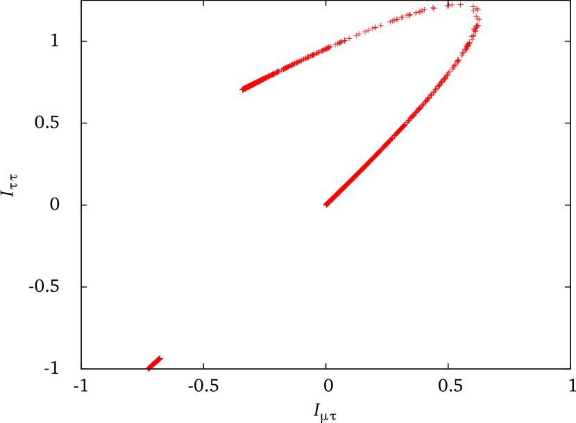
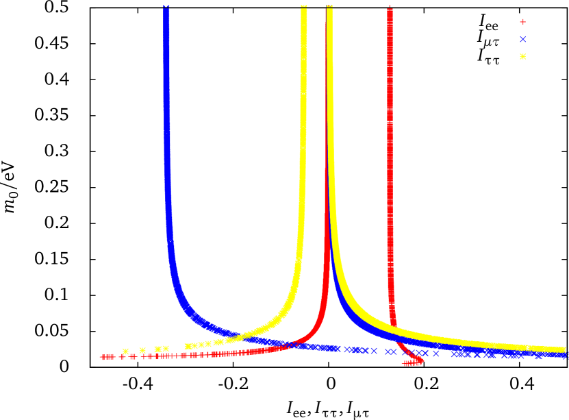
Figure 1: The allowed ranges for $I_{\tauup\tauup}$ and $I_{\muup\tauup}$ for $\Delta m_{31}^{2}$ and $\Delta m_{21}^{2}$ within their $1\,\sigma$ ranges (the mixing angles are taken at the central values). The left plot shows the dependence on the lightest neutrino mass $m_{0}$ in the vertical direction. There is one class of solutions where all three non-vanishing elements of $\boldsymbol{I}$ are close to zero.

Examination of other configurations as $m_{1}=m_{2}=-m_{3}$ or $-m_{1}=m_{2}=m_{3}$ are qualitatively the same and can be treated analogously.

The exact degenerate case: $m_{1}^{(0)}=m_{2}^{(0)}=m_{3}^{(0)}$

Unlike the situation where one mass eigenvalue has a different sign and there is only one freedom of rotation (in the plane where both masses have the same sign), the exact degenerate case allows for three arbitrary rotations. Trivially, there is no mixing matrix at the tree-level and therefore it is interesting to figure out whether threshold corrections have the power to generate the mixing—and lift the degeneracy in masses.

In General, Eq. (2.2) is a complex symmetric matrix, where the first term is proportional to the unit matrix:

$$\boldsymbol{m}^{\nuup}=m\;\mathds{1}+m\begin{pmatrix}I_{11}&I_{12}&I_{13}\\ I_{12}&I_{22}&I_{23}\\ I_{13}&I_{23}&I_{33}\end{pmatrix},$$ (2.10)

and $m$ is the common neutrino mass. Obviously, $\boldsymbol{m}^{\nuup}$ is diagonalized by diagonalizing only the perturbation $\boldsymbol{I}$. Models of exact degeneration can be motivated from $\mathrm{SO}(3)$ or $\mathrm{SU}(3)$ symmetries—or finite subgroups of them. Eq. (2.10) is the starting point to derive the physical mixing matrix from the threshold corrections. To a very good approximation, the charged leptons do not receive sizable flavor changing corrections, so the re-diagonalization of the perturbed neutrino mass matrix gives directly the phenomenological leptonic mixing matrix $\boldsymbol{U}_{\mathrm{PMNS}}$ observed in charged current interactions. (We work in the charged lepton mass basis.)

The diagonal neutrino mass matrix is obtained by the use of Eq. (1.3)

$${\bar{\boldsymbol{m}}}^{\nuup}=\boldsymbol{U}(\theta_{12},\theta_{13},\theta_{23})^{\text{T}}\;\boldsymbol{m}^{\nuup}\;\boldsymbol{U}(\theta_{12},\theta_{13},\theta_{23})=\boldsymbol{U}_{12}^{\text{T}}\boldsymbol{U}_{13}^{\text{T}}\boldsymbol{U}_{23}^{\text{T}}\boldsymbol{m}^{\nuup}\boldsymbol{U}_{23}\boldsymbol{U}_{13}\boldsymbol{U}_{12},$$ (2.11)

which shows that in the standard parametrization $\boldsymbol{U}_{23}$ acts “first” on the full mass matrix $\boldsymbol{m}^{\nuup}$. Note that for different parametrizations, especially a different ordering of rotations, the assignments to the measured angles are different and first have to be re-expressed by the standard angles. Eq. (1.3) as mixing matrix allows to directly apply the results of Ref. [38] and similar results to our problem.

Experimentally, $\theta_{23}$, the atmospheric mixing angle, is measured to be roughly maximal $|\theta_{23}|\approx\frac{\pi}{4}$ with a small deviation of a few degrees. The rotation angle in the $i$-$j$ plane can be expressed analytically in terms of the matrix elements via

$$\tan 2\theta_{ij}=\frac{2I_{ij}}{I_{jj}-I_{ii}},$$ (2.12)

where $\theta_{ij}$ can be chosen such that $0\leq\theta_{ij}\leq\pi/4$ by reordering diagonals and off-diagonals and shifting the the phase in the two-fold transformation

$$\boldsymbol{U_{ij}}(\theta_{ij},\delta_{ij})=\begin{pmatrix}\cos\theta_{ij}&\sin\theta_{ij}e^{-\mathrm{i}\,\delta_{ij}}\\ -\sin\theta_{ij}e^{\mathrm{i}\,\delta_{ij}}&\cos\theta_{ij}\end{pmatrix}.$$

Maximal mixing in the 2-3 plane means, that this sector can be diagonalized using

$$\boldsymbol{U}_{23}=\begin{pmatrix}1&0&0\\ 0&\frac{1}{\sqrt{2}}&-\frac{1}{\sqrt{2}}\\ 0&\frac{1}{\sqrt{2}}&\frac{1}{\sqrt{2}}\end{pmatrix},$$

by setting $I_{33}=I_{22}$ in Eq. (2.10). For simplicity and because it only has an influence on the resulting eigenvalues which can be absorbed in a redefinition of the mass parameter $m$, we also take $I_{23}=I_{22}$ (note that this is not required for $\theta_{23}=\pi/4$ and we release this requirement later). As result, we get

$$\boldsymbol{I}^{\prime}=\boldsymbol{U}^{\text{T}}_{23}\;\boldsymbol{I}\;\boldsymbol{U}_{23}=\begin{pmatrix}I_{11}&\frac{I_{12}+I_{13}}{\sqrt{2}}&-\frac{I_{12}-I_{13}}{\sqrt{2}}\\ \frac{I_{12}+I_{13}}{\sqrt{2}}&2I_{22}&0\\ -\frac{I_{12}-I_{13}}{\sqrt{2}}&0&0\end{pmatrix}.$$ (2.13)

Since a few years ago, the measured value of $\theta_{13}$ was comparable to zero, which suggests furthermore the approximation $I_{13}\approx I_{12}$ such that the last rotation is given by

$$\theta_{12}\approx\frac{1}{2}\arctan\left(\frac{2\sqrt{2}I_{12}}{2I_{22}-I_{11}}\right)$$ (2.14)

and the eigenvalues of $\boldsymbol{m}^{\nuup}$ are $m_{3}=m$ and

$$m_{1,2}=m\left\{1+\frac{1}{2}\left[I_{11}+2I_{22}\pm\left(I_{11}-2I_{22}\right)\sqrt{\frac{(I_{11}-2I_{22})^{2}+8I_{12}^{2}}{(I_{11}-2I_{22})^{2}}}\right]\right\}.$$ (2.15)

The mass squared differences calculated from the masses in (2.15) can be obtained as

$$\Delta m_{21}^{2} =m^{2}\left(2+I_{11}+2I_{22}\right)\left(2I_{22}-I_{11}\right)\sqrt{1+\frac{8I_{12}^{2}}{\left(I_{11}-2I_{22}\right)^{2}}},$$ (2.16)

$$\Delta m_{31}^{2} =-\frac{m^{2}}{2}\Bigg{[}\left(I_{11}(I_{11}+2)-I_{22}(I_{22}+1)\right)\sqrt{\frac{\left(I_{11}-2I_{22}\right)^{2}+8I_{12}^{2}}{(I_{11}-2I_{22})^{2}}}$$

$$\qquad\qquad\;+I_{11}\left(I_{11}+2\right)+I_{22}\left(I_{22}+1\right)+4I_{12}^{2}\Bigg{]}.$$

Altogether, there are four free parameters left ($m$, $I_{11}$, $I_{22}$ and $I_{12}$) required for fitting three masses and one mixing angle ($\theta_{12}$). The other two mixing angles were set to phenomenologically motivated distinct values ($\theta_{13}=0$ and $\theta_{23}=-\pi/4$) and shall receive small corrections in the following.

Up to now, we have set the third mixing angle to zero, which is disfavored by current experimental data. Nevertheless, we want to take the observed pattern in the quantum corrections as starting point to evaluate deviations from that by assigning deviations to the two restrictions that were set explicitly:

$$I_{33} =I_{22}+\varepsilon,$$ (2.17)

$$I_{13} =I_{12}+\delta,$$

with $\varepsilon,\delta$ parametrizing the deviations. As we will see, $\varepsilon$ and $\delta$ do not necessarily have to be small compared to $I_{12}$ and $I_{22}$. Especially the deviation in $I_{33}$ has to be of the same order as $I_{22}$. In that way, we now have six parameters ($I_{11}$, $I_{22}$, $I_{12}$, $I_{23}$, $\delta$ and $\varepsilon$) to completely fit three masses and three mixing angles, where $\theta_{23}$ is expected to be close to $\frac{\pi}{4}$ and $\theta_{13}$ small. We assign the “unperturbed” mass parameter to be $m=m_{0}$, any flavor-universal contribution in the threshold corrections can be simply added as a shift in the diagonals: $\tilde{I}_{\alpha}=I_{\alpha}-I_{0}$ for $\alpha=\mathrm{e},\muup,\tauup$. The relation between the observed masses and the threshold corrections is given by

$$\begin{pmatrix}m_{0}&&\\ &\sqrt{m_{0}^{2}+\Delta m_{21}^{2}}&\\ &&\sqrt{m_{0}^{2}+\Delta m_{31}^{2}}\end{pmatrix}$$ (2.18)

$$\qquad=m_{0}\,\boldsymbol{U}(\theta_{12},\theta_{13},\theta_{23})^{\text{T}}\begin{pmatrix}1+I_{11}&I_{12}&I_{12}+\delta\\ I_{12}&1+I_{22}&I_{23}\\ I_{12}+\delta&I_{23}&1+I_{22}+\varepsilon\end{pmatrix}\boldsymbol{U}(\theta_{12},\theta_{13},\theta_{23}),$$

where the mixing angles $\theta_{ij}$ and mass squared differences are fixed by experiment. For the numerical values, we refer to the global fit from the $\nu$-fit collaboration [38], where we now focus on the central value as a proof of principle:

$$\theta_{12}\approx 31.8^{\circ}\;,\;\theta_{13} \approx 8.5^{\circ}\;,\;\theta_{23}\approx 39.2^{\circ}\;,$$

$$\Delta m_{21}^{2}\approx 7.5\times 10^{-5}\,\mathrm{eV}^{2} ,\;\Delta m_{31}^{2}\approx 2.458\times 10^{-3}\,\mathrm{eV}^{2}.$$

The lightest neutrino mass $m_{0}$ is in principle a free parameter that will be tested by future neutrino mass experiments. Even if $m_{0}$ is not large enough to be directly measured, we show that quantum corrections still can lift the degenerate mass pattern sufficiently. Therefore we compare the two cases where either a positive direct determination is to be expected ($m_{0}=0.35\,\mathrm{eV}$) and the cosmologically favored ($m_{0}=0.1\,\mathrm{eV}$). The second value is still compatible within about $1\,\sigma$ with the $95\,\%$ upper bound on $\sum m_{\nu}$ and the nonzero value from galaxy clustering and lensing [4, 5].

Table 1: Values of the threshold corrections needed to obtain the observed mixing angles and mass splitting for a common neutrino mass of $0.1\,\mathrm{eV}$ and $0.35\,\mathrm{eV}$.

	$m_{0}=0.1\,\mathrm{eV}$	$m_{0}=0.35\,\mathrm{eV}$
$I_{11}$	$3.54\times 10^{-3}$	$3.00\times 10^{-4}$
$I_{12}$	$1.19\times 10^{-2}$	$1.02\times 10^{-3}$
$I_{22}$	$4.67\times 10^{-2}$	$4.01\times 10^{-3}$
$I_{23}$	$5.43\times 10^{-2}$	$4.67\times 10^{-3}$
$\varepsilon$	$2.28\times 10^{-2}$	$1.96\times 10^{-2}$
$\delta$	$6.73\times 10^{-5}$	$1.56\times 10^{-5}$
$\boldsymbol{I}$	$\qquad\begin{pmatrix}0.354&1.19&1.20\\ 1.19&4.67&5.43\\ 1.20&5.43&6.96\end{pmatrix}\times 10^{-2}$	$\qquad\begin{pmatrix}0.300&1.02&1.03\\ 1.02&4.01&4.67\\ 1.03&4.67&5.97\end{pmatrix}\times 10^{-3}$

The results are shown in Tab. 1 where we compare the two scenarios of a cosmologically inspired quasi-degenerate spectrum and a strong degeneracy as would follow from a KATRIN neutrino mass measurement. It is amusing to see that the entries of $\boldsymbol{I}$ are in both cases of the size of a typical radiative correction $\lesssim\mathcal{O}(1/100)$ (note that we only wanted to generate tiny deviations from the degenerate pattern in a regime where the physical masses are only slightly non-degenerate) and show a hierarchy as $1<2<3$ for labeling the generations. This observation can be used in any new physics model with flavor changing low-energy threshold corrections. An interesting model is presented in the next section, where we apply the concept of radiative generation of neutrino mixing and mass differences to an extension of the Minimal Supersymmetric Standard Model (MSSM). The complete contributions in the MSSM were already calculated and rather lengthy [39]. We are only interested in the contributions from Supersymmetry breaking, therefore we work with a reduced set of threshold corrections. Although we do not refer to any flavor symmetry, there are models with a high-energy non-abelian symmetry as $A_{4}$ with degenerate masses where the mass splitting and corrections to the mixing angles also happen radiatively [40, 41].

A crucial point in the discussion is the behavior of the generic threshold corrections with the lightest neutrino mass. In case the overall mass scale $m_{0}$ drops below $0.1\,\mathrm{eV}$, the spectrum looses the degenerate property which is expressed in values $I_{\alpha\beta}\simeq 0.1$ as can be seen in Fig. 2. Corrections are needed that are not of the size of typical perturbative corrections. The hierarchical regime ($m_{0}\ll 0.1\,\mathrm{eV}$) needs a special kind of flavor symmetry breaking where the degenerate patterns only needs a symmetry that guarantees equal masses. For a given symmetry breaking chain, the hierarchy can be exploited to construct the mixing matrix out of the mass ratios [42].

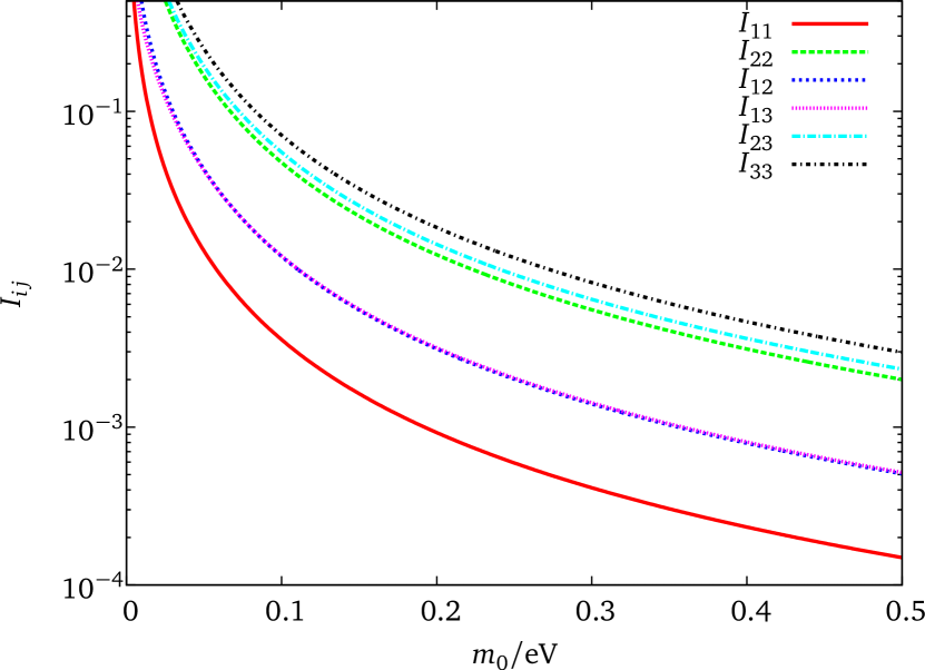
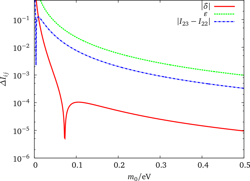
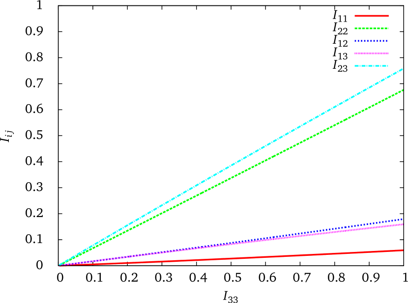
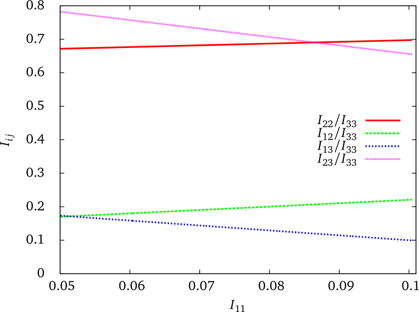
Figure 2: Graphical representation of the individual corrections. The first row shows the dependence on the absolute neutrino mass scale: the larger $m_{0}$ the smaller the corrections can be. The upper right plot shows the deviations from equal values: $\delta=I_{13}-I_{12}$ and $\varepsilon=I_{33}-I_{22}$ es defined in Eq. (2.17). The lower line shows the interplay of the individual $I_{jk}$ compared to $I_{33}$, similar plots can be done for other combinations. The lower right plot shows the $I_{jk}$ normalized to the largest contribution $I_{33}$.

3 A viable example: threshold corrections in the $\nuup$MSSM without minimal flavor violation

The MSSM is known to come along with many new sources of flavor violation in general. Incorporating the type-I seesaw mechanism to arrive at the dimension five operator (1.4) allows for an arbitrary flavor pattern arising at the loop-level even if some symmetry preserves flavor blind (and therefore degenerate) patterns at the tree-level. We will denote the seesaw-extension of the MSSM which is described in the following by $\nuup$MSSM.

Let us, for aesthetic reasons, introduce the same number of right-handed neutrino superfields as there are left-handed $\mathrm{SU}(2)$ doublets. Right-handed neutrinos are singlets under the SM gauge group which allows to acquire a Majorana mass term by some not further specified mechanism at the high scale $M_{\mathrm{R}}$.

The relevant part for neutrino physics of the $\nuup$MSSM is given by the superpotential

$$\mathcal{W}\;\supset \mu H_{1}\cdot H_{2}+Y^{\nuup}_{ij}\;H_{2}\cdot L_{\mathrm{L},i}N_{\mathrm{R},j}$$ (3.1)

$$-Y^{\ell}_{ij}\;H_{1}\cdot L_{\mathrm{L},i}E_{\mathrm{R},j}+\frac{1}{2}M^{\mathrm{R}}_{ij}N_{\mathrm{R},i}N_{\mathrm{R},j},$$

where we have the two Higgs $\mathrm{SU}(2)$ doublets $H_{1}=(h_{1}^{0},h_{1}^{-})$ and $H_{2}=(h_{2}^{+},h_{2}^{0})$, and the dot product denotes $\mathrm{SU}(2)$-invariant multiplication. The doublet of left-handed leptons is written as $L_{\mathrm{L}}=(N_{\mathrm{L}},E_{\mathrm{L}})$, where capital letters denote chiral superfields $F=\{\tilde{f},f\}$ and the right-handed matter fields are contained in the left-chiral multiplets $E_{\mathrm{R}}=\{\tilde{\ell}^{*}_{\mathrm{R}},\ell_{\mathrm{R}}^{c}\}$ and $N_{\mathrm{R}}=\{\tilde{\nu}^{*}_{\mathrm{R}},\nu^{c}_{\mathrm{R}}\}$. Generation indices $i,j$ are used in an obvious manner, $f^{c}$ is the charge conjugated fermion component.

To break Supersymmetry (SUSY) softly, we introduce the following potential terms

$$V_{\mathrm{soft}}^{\tilde{\nu}}=\left(\boldsymbol{m}_{\tilde{}\mathrm{L}}^{2}\right)_{ij}\tilde{\nu}_{\mathrm{L},i}^{*}\tilde{\nu}_{\mathrm{L},j}+\left(\boldsymbol{m}_{\tilde{}\mathrm{R}}^{2}\right)_{ij}\tilde{\nu}_{\mathrm{R},i}\tilde{\nu}^{*}_{\mathrm{R},j}+\left(A^{\nuup}_{ij}\;h_{2}^{0}\,\tilde{\nu}_{\mathrm{L},i}\tilde{\nu}_{\mathrm{R},j}^{*}+\left(\boldsymbol{B}^{2}\right)_{ij}\tilde{\nu}_{\mathrm{R},i}^{*}\tilde{\nu}_{\mathrm{R},j}^{*}+\text{h.\,c.\ }\right).$$ (3.2)

The neutrino $B$ term is written in a way that suggests no connection to $M_{\mathrm{R}}$ although it can be seen as a “Majorana-like” soft breaking mass term (therefore denoted here as $\boldsymbol{B}^{2}$). The usual way to write it down in the literature is rather $\boldsymbol{B}^{2}=b\,\boldsymbol{M}_{\mathrm{R}}$ with $b$ being a parameter of the SUSY scale, see e.g. [43, 44, 45].

In general, $\boldsymbol{A}^{\nuup}$ as well as $\boldsymbol{B}^{2}$ are arbitrary matrices in flavor space ($\boldsymbol{B}^{2}$ is symmetric). Because flavor-off-diagonal entries in the soft breaking mass $\boldsymbol{m}_{\tilde{}\mathrm{L}}^{2}$ easily lead to large FCNC processes in charged lepton physics, we take this contribution flavor blind as well as $\boldsymbol{m}_{\tilde{}\mathrm{R}}^{2}$:

$$\boldsymbol{m}_{\tilde{}\mathrm{L}}^{2}=\boldsymbol{m}_{\tilde{}\mathrm{R}}^{2}=M_{\mathrm{SUSY}}^{2}\,\mathds{1}.$$

Without loss of generality, we work in a basis where the charged lepton Yukawa coupling as well as the right-handed Majorana mass is diagonal. The neutrino Yukawa coupling can then be expressed in terms of the right-handed masses $M^{\mathrm{R}}_{i}$, the light neutrino masses $m^{\nuup}_{i}=v_{\mathrm{u}}^{2}\kappa_{i}$ and the PMNS matrix [46]:

$$\boldsymbol{Y}_{\nuup}=\sqrt{\boldsymbol{M}_{\mathrm{R}}}\mathcal{R}\sqrt{\boldsymbol{\kappa}}\boldsymbol{U}_{\mathrm{PMNS}}^{\dagger},$$ (3.3)

with $\mathcal{R}$ being an (arbitrary) complex orthogonal matrix. The Matrices $\sqrt{\boldsymbol{M}_{\mathrm{R}}}$ and $\sqrt{\boldsymbol{\kappa}}$ are diagonal matrices of the heavy and light masses, respectively. The right-handed Majorana mass scale $M_{\mathrm{R}}$ is a priori not constrained, where limits can be set from leptogenesis [47]. To get $\mathcal{O}(1)$ neutrino Yukawa couplings, we set $M_{\mathrm{R}}=10^{14}\,\mathrm{GeV}$.

Unfortunately, Eq. (3.3) allows for random flavor structures in $\boldsymbol{Y}_{\nuup}$ due to $\mathcal{R}$ which actually do not affect the tree-level mass and mixing formulae. Without any restrictions on $\boldsymbol{Y}_{\nuup}$, any prediction on the flavor mixing behavior of SUSY threshold corrections would be useless, because not only the combination $\boldsymbol{Y}_{\nuup}^{\text{T}}\boldsymbol{M}_{\mathrm{R}}^{-1}\boldsymbol{Y}_{\nuup}$ will appear but also $\boldsymbol{A}^{\nuup}\boldsymbol{Y}_{\nuup}$ and $\boldsymbol{M}_{\mathrm{R}}\boldsymbol{Y}_{\nuup}$.

Remember that we wanted to explain deviations from the degenerate neutrino mass pattern. Integrating out the heavy superfields in Eq. (3.1) brings us to the effective operator of Eq. (1.4) and yields a light neutrino mass matrix of the form

$$\boldsymbol{m}_{\nuup}^{(0)}=-v_{\mathrm{u}}^{2}\boldsymbol{Y}_{\nuup}^{\text{T}}\,\boldsymbol{M}_{\mathrm{R}}^{-1}\boldsymbol{Y}_{\nuup}+\mathcal{O}(v_{\mathrm{u}}^{4}/M_{\mathrm{R}}^{3}).$$ (3.4)

To get exact degeneracy in $\boldsymbol{m}_{\nuup}^{(0)}$ there has to be some conspiracy at work that adjusts $\boldsymbol{Y}_{\nuup}$ in a way to cope with any non-degenerate pattern in $\boldsymbol{M}_{\mathrm{R}}$. Avoiding any conspiracies, we assume (conspire?) the Yukawa coupling as well as the right-handed Majorana mass to be flavor blind: $\boldsymbol{Y}_{\nuup}=y_{\nuup}\,\mathds{1}$ and $\boldsymbol{M}_{\mathrm{R}}=m_{\mathrm{R}}\,\mathds{1}$. Other popular choices like

$$\boldsymbol{Y}_{\nuup}=\begin{pmatrix}1&0&0\\ 0&0&1\\ 0&1&0\end{pmatrix}$$

as favored by discrete flavor symmetries do not alter the qualitative features of the results. The degenerate neutrino mass is then given by $m=v_{\mathrm{u}}^{2}y_{\nuup}^{2}/m_{\mathrm{R}}$.

Calculation of the SUSY threshold corrections is done by evaluating the neutrino self-energies including superpartners [44]:

$$\left(\boldsymbol{m}_{\nuup}^{\mathrm{1-loop}}\right)_{ij}=\left(\boldsymbol{m}^{(0)}_{\nuup}\right)_{ij}+\operatorname{Re}\left[\Sigma^{(\nuup),\mathrm{S}}_{ij}+\frac{m^{(0)}_{\nuup_{i}}}{2}\Sigma^{(\nuup),\mathrm{V}}_{ij}+\frac{m^{(0)}_{\nuup_{j}}}{2}\Sigma^{(\nuup),\mathrm{V}}_{ji}\right],$$ (3.5)

with the decomposition of the neutrino self-energy

$$\Sigma^{(\nuup)}_{ij}(p)=\Sigma^{(\nuup),\mathrm{S}}_{ij}(p^{2})P_{\mathrm{L}}+{\Sigma^{(\nuup),\mathrm{S}}_{ij}}^{*}(p^{2})P_{\mathrm{R}}+\not{p}\left[{\Sigma^{(\nuup),\mathrm{V}}_{ij}}(p^{2})P_{\mathrm{L}}+{\Sigma^{(\nuup),\mathrm{V}}_{ij}}^{*}(p^{2})P_{\mathrm{R}}\right].$$ (3.6)

For Majorana neutrinos, the self-energy is flavor symmetric ($\Sigma_{ij}=\Sigma_{ji}$ and the coefficients in front of the left and right projectors ($P_{\mathrm{L}}$ and $P_{\mathrm{R}}$ respectively) are related via complex conjugation. We evaluate the self-energies at $p^{2}=0$ since the sparticles in the loop are superheavy compared to neutrinos.

The flavor changing scalar and vectorial parts of the neutrino self-energies according to Eq. (3.6) can be easily calculated—although the mixing matrices are only to be determined numerically:

$$\left(\boldsymbol{\Sigma}^{(\nuup),\mathrm{S}}\right)_{ij} =\frac{1}{4(2\pi)^{2}}B_{0}(m_{\tilde{\chi}_{k}^{0}},m_{\tilde{\nu}_{s}})m_{\tilde{\chi}_{k}^{0}}\left(\frac{-i}{\sqrt{2}}\right)^{2}\left(g_{2}Z^{\mathrm{N}}_{2k}-g_{1}Z^{\mathrm{N}}_{1k}\right)^{2}\mathcal{Z}^{\tilde{}\nuup*}_{i^{\prime}s}\mathcal{Z}^{\tilde{}\nuup*}_{j^{\prime}s}(\boldsymbol{U}_{\mathrm{PMNS}})_{i^{\prime}i}(\boldsymbol{U}_{\mathrm{PMNS}})_{j^{\prime}j},$$ (3.7a)

$$\left(\boldsymbol{\Sigma}^{(\nuup),\mathrm{V}}\right)_{ij} =\frac{1}{4(2\pi)^{2}}B_{1}(m_{\tilde{\chi}_{k}^{0}},m_{\tilde{\nu}_{s}})\left(\frac{-i}{\sqrt{2}}\right)^{2}\left|g_{2}Z^{\mathrm{N}}_{2k}-g_{1}Z^{\mathrm{N}}_{1k}\right|^{2}\mathcal{Z}^{\tilde{}\nuup}_{i^{\prime}s}\mathcal{Z}^{\tilde{}\nuup*}_{j^{\prime}s}(\boldsymbol{U}^{*}_{\mathrm{PMNS}})_{i^{\prime}i}(\boldsymbol{U}_{\mathrm{PMNS}})_{j^{\prime}j},$$ (3.7b)

where summation over repeated indices is understood. The unrenormalized neutrino mixing matrix which occurs in the vertex is denoted by $\boldsymbol{U}_{\mathrm{PMNS}}$, $\mathcal{Z}^{\tilde{}\nuup}$ is the slightly modified sneutrino mixing matrix described in the appendix B, $\boldsymbol{Z}^{\mathrm{N}}$ is the neutralino mixing matrix, $B_{0}$ and $B_{1}$ the emerging loop functions. The same expressions were found by the authors of [44] as well with the conventions of App. B.

We are restricting ourselves to only $\boldsymbol{A}^{\nuup}$ having an arbitrary flavor structure—and determine this structure by comparing the result of Eq. (3.5) by virtue of SUSY corrections to the solution of Eq. (2.18) where the size of the threshold corrections can be obtained as $m\,I_{ij}=\left(\boldsymbol{m}_{\nuup}^{\mathrm{1-loop}}\right)_{ij}-m\delta_{ij}$ with $m$ being the degenerate mass at tree-level. The dependence on the remaining SUSY parameters is quite mild in any respect. For the analysis presented here we vary the values of the following variables randomly in the given intervals:

$$M_{\mathrm{SUSY}} \in[500,5000]\,\mathrm{GeV},$$ (3.8)

$$M_{1} \in[0.3,3]\,M_{\mathrm{SUSY}},$$

$$M_{2} \in[1,5]\,M_{\mathrm{SUSY}},$$

$$\mu \in[-15,15]\,\mathrm{TeV},$$

$$\tan\beta \in[10,60].$$

As expected, for low values of the absolute neutrino mass $m_{0}$ where the deviation from the degenerate pattern is large, the SUSY threshold corrections measured in the values of $\boldsymbol{A}^{\nuup}$ have to be large as shown in Fig. 3 where we plotted the ratio $a_{ij}=A^{\nuup}_{ij}/M_{\mathrm{SUSY}}$. The left-hand side of Fig. 3 compared to the right-hand side shows that that basically this ratio is the parameter which drives the corrections and has the same shape as the $I_{ij}$ dependent on $m_{0}$ where the size of the $A^{\nuup}_{ij}$ depending on the SUSY scale also is sensitive to the parameters of the theory.

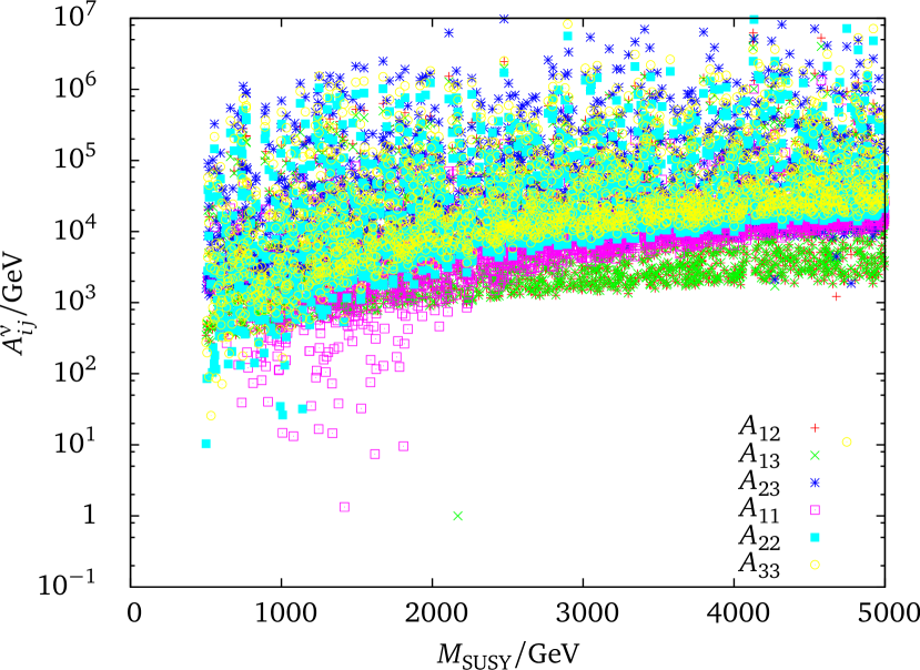
Figure 3: The left plot shows values of $\boldsymbol{A}^{\nuup}$ for the variation of parameters specified in (3.8). The lightest neutrino mass $m_{0}$ was chosen in the regime plotted on the right side, where we rescaled all trilinear soft breaking couplings with the SUSY scale, $a_{ij}=A^{\nuup}_{ij}/M_{\mathrm{SUSY}}$. The values of $a_{12}$ and $a_{13}$ are roughly the same since they differ only by a small parameter as described in Sec. 2.

The correlations between the $I_{ij}$ elaborated in Sec. 2 also get reflected to the trilinear SUSY breaking terms shown in Fig. 4. Especially the off-diagonals are very strongly correlated where we only expected this for $A^{\nuup}_{12}$ and $A^{\nuup}_{13}$. The least correlation can be seen between $A_{12}$ and $A_{11}$ which correspond to $I_{12}$ and $I_{11}$ that were seen to be the most independent contributions.

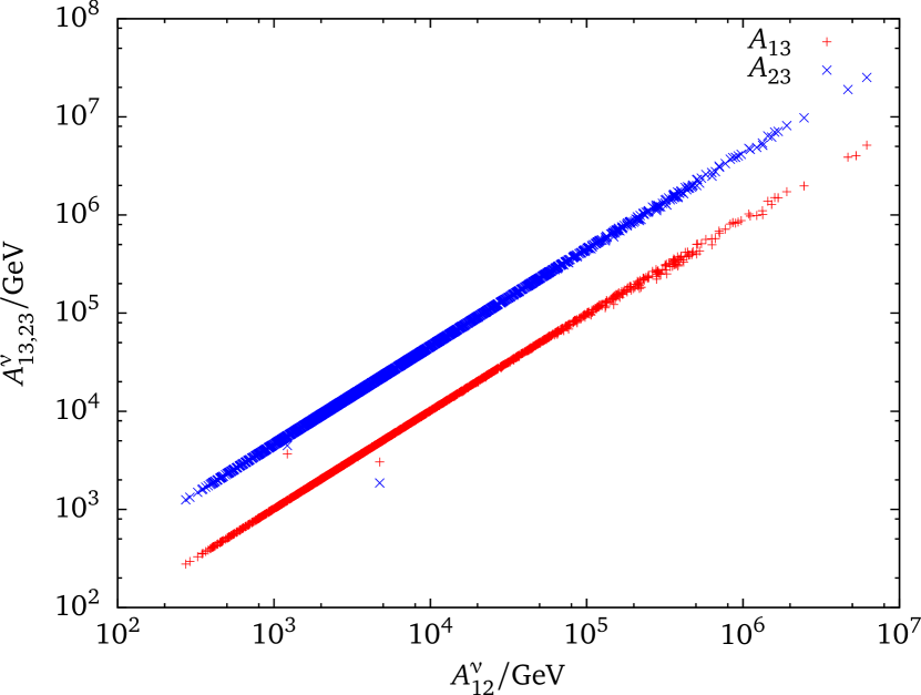
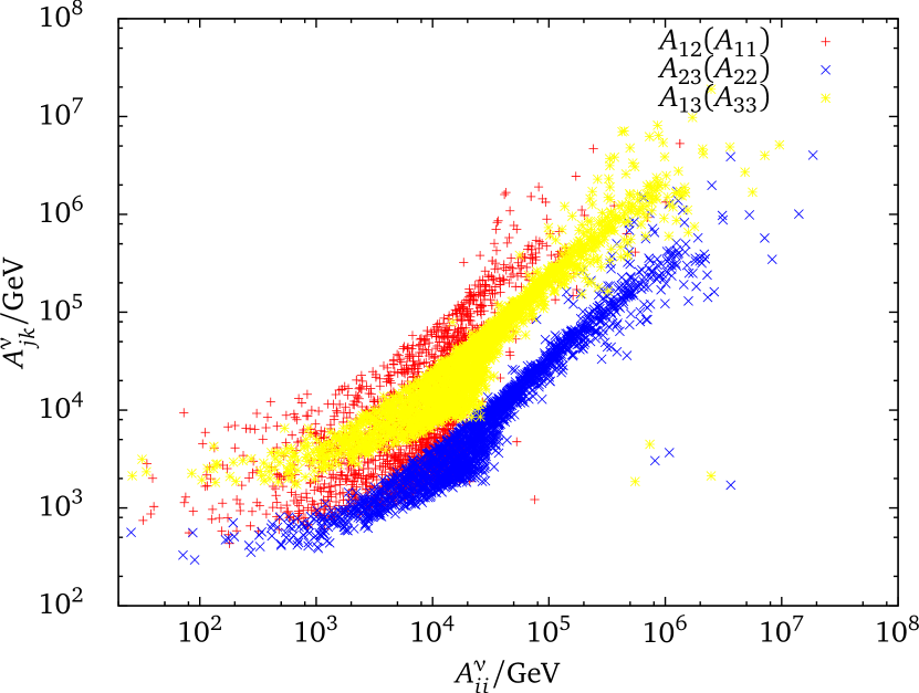
Figure 4: Correlations between the different elements of $\boldsymbol{A}^{\nuup}$. The left plot shows the off-diagonals with respect to $A^{\nuup}_{12}$ where the right shows the correlation with the diagonal entries.

4 Conclusions

We have discussed degenerate neutrino masses at the tree-level and showed how threshold corrections to the masses affect the mixing. The cosmologically favored value for the absolute neutrino mass is rather at the edge of what is usually called quasi-degenerate mass spectrum. In contrast, any direct measurement like from tritium decay would immediately pose a highly degenerate spectrum. Both degenerate cases imply that small threshold corrections arising at some scale between the electroweak and the scale of any UV complete theory are sufficient to generate both the neutrino mass spectrum as well as the mixing angles radiatively. For the general discussion, we have not fixed any model to account for neutrino masses and even neglected the RGE running down to the electroweak scale. RGE corrections are known to be important altering both mixing angles and mass differences considerably. Several degenerate patterns, however, are known to preserve specific mixing patterns.

We re-examined the more general possibility of neutrino mass eigenstates having different $\mathrm{CP}$ eigenvalues (when $\mathrm{CP}$ is conserved) which lead to a simplified description of threshold corrections. In this scenario, there exist non-trivial tree-level mixings and the task is to determine deviations from that. It is, however, impossible to simultaneously accommodate for both mass splittings and a sizable third mixing angle with only flavor-diagonal threshold corrections. We have to include at least one off-diagonal, $I_{\mu\tau}$, which is indeed sufficient to reproduce the masses and mixings in the interplay with the diagonal $I_{\mathrm{e}}$ and $I_{\tauup}$.

For the case of a trivial tree-level mixing with three exactly degenerate masses, we derived phenomenologically out of the observed neutrino mixing patterns (e.g nearly maximal $\theta_{23}$ whereas small $\theta_{13}$) constraints and correlations on the threshold corrections $I_{ij}$ that can help to survey the parameter space of the full theory. For degenerate neutrino masses, the typical size of the corrections is in the range of a one-loop threshold correction. In this spirit, we applied this method of degeneracy-lifting to threshold corrections as they typically occur in supersymmetric models including a theory of neutrino masses. The $\nuup$MSSM sets the stage of a very powerful model. Although in its full generality, no statements about any flavor pattern of the SUSY threshold corrections can ever be made, we transferred the principle of degeneracy to the potentially arbitrary parameters there and set the right-handed Majorana masses as well as the neutrino Dirac masses to a degenerate pattern. In this very limited setup, we looked for trilinear couplings $\boldsymbol{A}^{\nuup}$ fulfilling the requirements of the threshold corrections $I_{ij}$ to end up at the observed patterns of masses and mixings. The results are qualitatively very stable under variation of the free SUSY parameters. In any case, we need large neutrino $A$ terms to get the structure of the threshold corrections as for the generic discussion. Effectively, the combination $\boldsymbol{A}^{\nuup}/M_{\mathrm{SUSY}}$ drives the corrections.

Shifting the generation of neutrino flavor from the mass matrices to the soft SUSY breaking sector, especially $\boldsymbol{A}^{\nuup}$, does not solve the flavor puzzle neither reveals this procedure a deeper understanding. The possibility of flavor mixing arising as a pure quantum effect in the low energy effective theory, however, opens another view on the flavor puzzle. Breaking Supersymmetry in a way that does not respect flavor challenges also models for SUSY breaking. Even if the UV extension of the SM is not supersymmetric, the formulation of neutrino mixing via low-energy threshold corrections implies a theory of flavor hidden in the yet veiled new physics.

Appendix A Sneutrino squared mass matrix and mixing matrix

Extending the MSSM by right-handed neutrinos and giving them a Majorana mass leads to a seesaw-like mechanism in the sneutrino sector. Similar to the seesaw-extended Standard Model, where the neutrino spectrum gets doubled, the sneutrino spectrum gets quadrupled. Why that? The MSSM contains only three sneutrino states. Including right-handed fields, the number of states get doubled, although half of them are singlets under the SM gauge group. Moreover, due to Dirac and Majorana masses, the physical spectrum gets even more enlarged. Effectively, we are left with six light, more or less active states, and six heavy singlet-like states. A priori, the sneutrino squared mass matrix is therefore a $12\times 12$ matrix, which can be perturbatively block-diagonalised similar to the neutrino mass matrix. The complete procedure is described in great detail by [44].

We choose the following basis: $\tilde{N}=(\tilde{\nu}_{\mathrm{L}},\tilde{\nu}_{\mathrm{L}}^{*},\tilde{\nu}_{\mathrm{R}}^{*},\tilde{\nu}_{\mathrm{R}})^{\text{T}}$ (such that $-\mathcal{L}^{\tilde{}\nuup}_{\mathrm{mass}}=N^{\dagger}(\mathcal{M}_{\mathbf{\tilde{}\nuup}})^{2}N$) and classify chirality conserving ($LL,RR$) and chirality changing blocks:

$$(\mathcal{M}_{\mathbf{\tilde{\nu}}})^{2}=\frac{1}{2}\begin{pmatrix}\mathcal{M}_{LL}^{2}&\mathcal{M}_{LR}^{2}\\ \left(\mathcal{M}_{LR}^{2}\right)^{\dagger}&\mathcal{M}_{RR}^{2}\end{pmatrix},$$

with

$$\mathcal{M}_{LL}^{2} =\begin{pmatrix}\mathcal{M}_{\tilde{\ell}}^{2}+\frac{1}{2}M_{Z}^{2}\cos 2\beta\mathds{1}+\boldsymbol{m}^{\mathrm{D}}_{\nuup}{\boldsymbol{m}^{\mathrm{D}}_{\nuup}}^{\dagger}&\boldsymbol{0}\\ \boldsymbol{0}&(\mathcal{M}_{\tilde{\ell}}^{2})^{T}+\frac{1}{2}M_{Z}^{2}\cos 2\beta\mathds{1}+{\boldsymbol{m}^{\mathrm{D}}_{\nuup}}^{*}{\boldsymbol{m}^{\mathrm{D}}_{\nuup}}^{T}\end{pmatrix},$$ (A.1a)

$$\mathcal{M}_{RL}^{2} =\begin{pmatrix}\boldsymbol{m}^{\mathrm{D}}_{\nuup}\boldsymbol{M}_{\mathrm{R}}&-\mu\cot\beta\boldsymbol{m}^{\mathrm{D}}_{\nuup}+v_{\mathrm{u}}\boldsymbol{A}_{\nuup}^{*}\\ -\mu^{*}\cot\beta{\boldsymbol{m}^{\mathrm{D}}_{\nuup}}^{*}+v_{\mathrm{u}}\boldsymbol{A}_{\nuup}&{\boldsymbol{m}^{\mathrm{D}}_{\nuup}}^{*}\boldsymbol{M}_{\mathrm{R}}^{*}\end{pmatrix},$$ (A.1b)

$$\mathcal{M}_{RR}^{2} =\begin{pmatrix}(\mathcal{M}_{\tilde{}\nuup}^{2})^{T}+{\boldsymbol{m}^{\mathrm{D}}_{\nuup}}^{T}{\boldsymbol{m}^{\mathrm{D}}_{\nuup}}^{*}+\boldsymbol{M}_{\mathrm{R}}^{*}\boldsymbol{M}_{\mathrm{R}}&2(\boldsymbol{B}^{2})^{*}\\ 2\boldsymbol{B}^{2}&\mathcal{M}_{\tilde{}\nuup}^{2}+{\boldsymbol{m}^{\mathrm{D}}_{\nuup}}^{\dagger}\boldsymbol{m}^{\mathrm{D}}_{\nuup}+\boldsymbol{M}_{\mathrm{R}}\boldsymbol{M}^{*}_{\mathrm{R}}\end{pmatrix},$$ (A.1c)

where bold face symbols as well as the soft slepton masses $\mathcal{M}^{2}_{\tilde{\ell},\tilde{}\nuup}$ denote $3\times 3$ matrices in flavour space and the singlet mass is symmetric: $\boldsymbol{M}_{\mathrm{R}}=\boldsymbol{M}_{\mathrm{R}}^{T}$. And $\boldsymbol{m}^{\mathrm{D}}_{\nuup}$ is the Dirac neutrino mass matrix defined as $\boldsymbol{m}^{\mathrm{D}}_{\nuup}=\frac{1}{\sqrt{2}}v_{\mathrm{u}}\boldsymbol{Y}_{\nuup}$.

Appendix B Feynman rules for the type I seesaw-extended MSSM

The relevant vertices for the lepton flavor changing self energies are triple vertices for the lepton-slepton-gaugino and -higgsino interactions:

$$i\,\Gamma_{\nu_{f}}^{\tilde{\nu}_{s}\tilde{\chi}^{0}_{k}}=\, -\frac{i}{\sqrt{2}}\bigg{\{}\left[(g_{2}Z_{2k}^{\mathrm{N}}-g_{1}Z_{1k}^{\mathrm{N}})\mathcal{Z}^{\tilde{}\nuup*}_{is}(\boldsymbol{U}_{\mathrm{PMNS}})_{if}\right]P_{\mathrm{L}}$$ (B.1a)

$$\qquad\qquad+\left[(g_{2}Z_{2k}^{\mathrm{N}*}-g_{1}Z_{1k}^{\mathrm{N}*})\mathcal{Z}^{\tilde{}\nuup}_{is}(\boldsymbol{U}^{*}_{\mathrm{PMNS}})_{if}\right]P_{\mathrm{R}}\bigg{\}},$$

$$i\,\Gamma_{e_{i}}^{\tilde{e}_{s}\tilde{\chi}^{0}_{k}}=\, \frac{i}{\sqrt{2}}\bigg{\{}\left((g_{2}Z_{2k}^{\mathrm{N}}+g_{1}Z_{1k}^{\mathrm{N}})W^{\tilde{}\mathrm{e}}_{is}-y_{ij}^{\mathrm{e}}Z_{3k}^{\mathrm{N}}W^{\tilde{}\mathrm{e}}_{j+3,s}\right)P_{\mathrm{L}}$$ (B.1b)

$$\qquad\qquad-\left(\sqrt{2}g_{1}Z_{1k}^{\mathrm{N}}W^{\tilde{}\mathrm{e}}_{i+3,s}+y_{ji}^{\mathrm{e}*}Z_{3k}^{\mathrm{N}}W^{\tilde{}\mathrm{e}}_{js}\right)P_{\mathrm{R}}\bigg{\}},$$

$$i\,\Gamma_{\nu_{f}}^{\tilde{e}_{s}\tilde{\chi}^{+}_{k}}=\, -i\left[g_{2}Z_{1k}^{-}W^{\tilde{}\mathrm{e}*}_{is}-y_{ij}^{\mathrm{e}*}Z_{2k}^{-}W^{\tilde{}\mathrm{e}*}_{j+3,s}\right](\boldsymbol{U}_{\mathrm{PMNS}})_{if}P_{\mathrm{L}},$$ (B.1c)

$$i\,\Gamma_{e_{i}}^{\tilde{\nu}_{s}\left(\tilde{\chi}^{+}_{k}\right)^{c}}=\, -i\left[g_{2}Z_{1k}^{+}\mathcal{Z}^{\tilde{}\nuup*}_{i,s}P_{\mathrm{L}}-y_{ij}^{\mathrm{e}}Z_{2k}^{-*}\mathcal{Z}^{\tilde{}\nuup}_{js}P_{\mathrm{R}}\right],$$ (B.1d)

where summation over double indices is understood.

The vertices of eqs. (B.1) are given for an incoming standard model fermion, outgoing chargino or neutralino as well as sfermion. They generically follow from a interaction Lagrangian like

$$\mathcal{L}_{\mathrm{int}}=\bar{f}_{i}\,\Gamma^{\tilde{f}_{s}\tilde{\chi}_{k}}_{f_{f}}\;\tilde{\chi}_{k}\,\tilde{f}_{f}\,+\mathrm{\ h.\ c.}$$

Each vertex comes along with the corresponding chirality projector:

$$\Gamma^{\tilde{f}_{s}\tilde{\chi}_{k}}_{f_{f}}=\Gamma^{\tilde{f}_{s}\tilde{\chi}_{k}}_{\mathrm{L},f_{f}}P_{\mathrm{L}}+\Gamma^{\tilde{f}_{s}\tilde{\chi}_{k}}_{\mathrm{R},f_{f}}P_{\mathrm{R}}$$

The mixing matrices diagonalize the mass matrices in the following manner:

• Chargino mixing: $\boldsymbol{Z}^{-\text{T}}\mathcal{M}_{\mathrm{C}}\boldsymbol{Z}^{+}=\left(\mathcal{M}_{\mathrm{C}}\right)^{\mathrm{diag}}$,

• Neutralino mixing: $\boldsymbol{Z}^{\mathrm{N}\text{T}}\mathcal{M}_{\mathrm{N}}\boldsymbol{Z}^{\mathrm{N}}=\left(\mathcal{M}_{\mathrm{N}}\right)^{\mathrm{diag}}$,

• Slepton mixing: $\boldsymbol{W}^{\tilde{}\mathrm{e}{\dagger}}\mathcal{M}^{2}_{\tilde{}\mathrm{e}}\boldsymbol{W}^{\tilde{}\mathrm{e}}=\left(\mathcal{M}^{2}_{\tilde{}\mathrm{e}}\right)^{\mathrm{diag}}$,

• Sneutrino mixing:

  $$\mathcal{W}^{\tilde{}\nuup{\dagger}}\bar{\mathcal{M}}_{\tilde{}\nuup}^{2}\mathcal{W}^{\tilde{}\nuup}=\mathcal{W}^{\tilde{}\nuup{\dagger}}\mathcal{P}^{\dagger}\mathcal{M}_{\tilde{}\nuup}^{2}\mathcal{P}\mathcal{W}^{\tilde{}\nuup}=\left(\mathcal{M}^{2}_{\tilde{}\nuup}\right)^{\mathrm{diag}},$$

  such that $\mathcal{Z}^{\tilde{}\nuup}=\mathcal{P}\mathcal{W}^{\tilde{}\nuup}$ diagonalizes the original mass matrix $\mathcal{M}^{2}_{\tilde{}\nuup}$ and therefore:

  $$\mathcal{Z}_{is}^{\tilde{}\nuup} =\frac{1}{\sqrt{2}}\left(\mathcal{W}_{is}^{\tilde{}\nuup}+i\mathcal{W}_{i+3,s}^{\tilde{}\nuup}\right)\quad\text{and}$$

  $$\mathcal{Z}_{i+3,s}^{\tilde{}\nuup} =\frac{1}{\sqrt{2}}\left(\mathcal{W}_{is}^{\tilde{}\nuup}-i\mathcal{W}_{i+3,s}^{\tilde{}\nuup}\right)$$

  appear in the vertices of eqs. (B.1).

• Neutrino mixing: The PMNS mixing matrix can be determined from the neutrino mass matrix $\boldsymbol{m}_{\nuup}^{\mathrm{diag}}=\boldsymbol{U}_{\mathrm{PMNS}}^{*}\boldsymbol{m}_{\nuup}\boldsymbol{U}_{\mathrm{PMNS}}^{\dagger}$, where $m_{\nuup}$ is the effective light neutrino mass matrix and the charged lepton masses can be taken diagonal (otherwise there would be a contribution to the PMNS mixing similar to the CKM mixing from both up and down sector: $\boldsymbol{U}_{\mathrm{PMNS}}=\boldsymbol{V}_{\mathrm{e},\mathrm{L}}^{\dagger}\boldsymbol{U}_{\nuup,\mathrm{L}}$, where $\boldsymbol{V}_{\mathrm{e},\mathrm{L}}$ rotates the left-handed electron fields).

Loop functions

Finally, we give our conventions for the arising $\overline{\mathrm{MS}}$ subtracted loop functions for $p^{2}=0$ and $\mu_{r}$ the renormalization scale:

$$B_{0}(m_{1},m_{2}) =-\ln\frac{m_{1}m_{2}}{\mu_{r}^{2}}+1-\frac{m_{1}^{2}+m_{2}^{2}}{m_{1}^{2}-m_{2}^{2}}\ln\frac{m_{1}}{m_{2}},$$ (B.2a)

$$B_{1}(m_{1},m_{2}) =\frac{1}{2}\ln\frac{m_{1}m_{2}}{\mu_{r}^{2}}-\frac{3}{4}-\frac{m_{2}^{2}}{2(m_{1}^{2}-m_{2}^{2})}+\left(\frac{m_{1}^{4}}{(m_{1}^{2}-m_{2}^{2})^{2}}-\frac{1}{2}\right)\frac{m_{1}}{m_{2}}.$$ (B.2b)

References

- [1] KATRIN Collaboration, A. Osipowicz et al., “KATRIN: A Next generation tritium beta decay experiment with sub-eV sensitivity for the electron neutrino mass. Letter of intent,” arXiv:hep-ex/0109033 [hep-ex].
- [2] K. Abazajian, E. Calabrese, A. Cooray, F. De Bernardis, S. Dodelson, et al., “Cosmological and Astrophysical Neutrino Mass Measurements,” Astropart.Phys. 35 (2011) 177–184, arXiv:1103.5083 [astro-ph.CO].
- [3] K. Abazajian et al., “Neutrino Physics from the Cosmic Microwave Background and Large Scale Structure,” Astropart.Phys. 63 (2014) 66–80, arXiv:1309.5383 [astro-ph.CO].
- [4] Planck Collaboration, P. Ade et al., “Planck 2013 results. XVI. Cosmological parameters,” Astron.Astrophys. (2014) , arXiv:1303.5076 [astro-ph.CO].
- [5] R. A. Battye and A. Moss, “Evidence for Massive Neutrinos from Cosmic Microwave Background and Lensing Observations,” Phys.Rev.Lett. 112 no. 5, (2014) 051303, arXiv:1308.5870 [astro-ph.CO].
- [6] M. Gonzalez-Garcia, M. Maltoni, and T. Schwetz, “Updated fit to three neutrino mixing: status of leptonic CP violation,” arXiv:1409.5439 [hep-ph].
- [7] J. R. Ellis and S. Lola, “Can neutrinos be degenerate in mass?,” Phys.Lett. B458 (1999) 310–321, arXiv:hep-ph/9904279 [hep-ph].
- [8] J. Casas, J. Espinosa, A. Ibarra, and I. Navarro, “Naturalness of nearly degenerate neutrinos,” Nucl.Phys. B556 (1999) 3–22, arXiv:hep-ph/9904395 [hep-ph].
- [9] J. Casas, J. Espinosa, A. Ibarra, and I. Navarro, “Nearly degenerate neutrinos, supersymmetry and radiative corrections,” Nucl.Phys. B569 (2000) 82–106, arXiv:hep-ph/9905381 [hep-ph].
- [10] N. Haba, Y. Matsui, N. Okamura, and M. Sugiura, “The Effect of Majorana phase in degenerate neutrinos,” Prog.Theor.Phys. 103 (2000) 145–150, arXiv:hep-ph/9908429 [hep-ph].
- [11] E. J. Chun and S. Pokorski, “Slepton flavor mixing and neutrino masses,” Phys.Rev. D62 (2000) 053001, arXiv:hep-ph/9912210 [hep-ph].
- [12] K. Balaji, A. S. Dighe, R. Mohapatra, and M. Parida, “Generation of large flavor mixing from radiative corrections,” Phys.Rev.Lett. 84 (2000) 5034–5037, arXiv:hep-ph/0001310 [hep-ph].
- [13] P. H. Chankowski, A. Ioannisian, S. Pokorski, and J. Valle, “Neutrino unification,” Phys.Rev.Lett. 86 (2001) 3488–3491, arXiv:hep-ph/0011150 [hep-ph].
- [14] E. J. Chun, “Lepton flavor violation and radiative neutrino masses,” Phys.Lett. B505 (2001) 155–160, arXiv:hep-ph/0101170 [hep-ph].
- [15] P. H. Chankowski and S. Pokorski, “Quantum corrections to neutrino masses and mixing angles,” Int.J.Mod.Phys. A17 (2002) 575–614, arXiv:hep-ph/0110249 [hep-ph].
- [16] R. Mohapatra, M. Parida, and G. Rajasekaran, “High scale mixing unification and large neutrino mixing angles,” Phys.Rev. D69 (2004) 053007, arXiv:hep-ph/0301234 [hep-ph].
- [17] B. Brahmachari and E. J. Chun, “Supersymmetric threshold corrections to ,” Phys.Lett. B596 (2004) 184–190, arXiv:hep-ph/0312030 [hep-ph].
- [18] R. Mohapatra, M. Parida, and G. Rajasekaran, “Threshold effects on quasi-degenerate neutrinos with high-scale mixing unification,” Phys.Rev. D71 (2005) 057301, arXiv:hep-ph/0501275 [hep-ph].
- [19] N. Haba and R. Takahashi, “Grand Unification of Flavor Mixings,” Europhys.Lett. 100 (2012) 31001, arXiv:1206.2793 [hep-ph].
- [20] P. Minkowski, “ at a Rate of One Out of 1-Billion Muon Decays?,” Phys.Lett. B67 (1977) 421.
- [21] R. N. Mohapatra and G. Senjanovic, “Neutrino Mass and Spontaneous Parity Violation,” Phys.Rev.Lett. 44 (1980) 912.
- [22] T. Yanagida, “Horizontal Symmetry and Masses of Neutrinos,” Prog.Theor.Phys. 64 (1980) 1103.
- [23] M. Gell-Mann, P. Ramond, and R. Slansky, “Complex Spinors and Unified Theories,” Conf.Proc. C790927 (1979) 315–321, arXiv:1306.4669 [hep-th].
- [24] J. Schechter and J. Valle, “Neutrino Masses in SU(2) x U(1) Theories,” Phys.Rev. D22 (1980) 2227.
- [25] M. Magg and C. Wetterich, “Neutrino Mass Problem and Gauge Hierarchy,” Phys.Lett. B94 (1980) 61.
- [26] J. Schechter and J. Valle, “Neutrino Decay and Spontaneous Violation of Lepton Number,” Phys.Rev. D25 (1982) 774.
- [27] S. Weinberg, “Baryon and Lepton Nonconserving Processes,” Phys.Rev.Lett. 43 (1979) 1566–1570.
- [28] B. Pontecorvo, “Inverse beta processes and nonconservation of lepton charge,” Sov.Phys.JETP 7 (1958) 172–173.
- [29] Z. Maki, M. Nakagawa, and S. Sakata, “Remarks on the unified model of elementary particles,” Prog.Theor.Phys. 28 (1962) 870–880.
- [30] P. H. Chankowski and Z. Pluciennik, “Renormalization group equations for seesaw neutrino masses,” Phys.Lett. B316 (1993) 312–317, arXiv:hep-ph/9306333 [hep-ph].
- [31] N. Haba, N. Okamura, and M. Sugiura, “The Renormalization group analysis of the large lepton flavor mixing and the neutrino mass,” Prog.Theor.Phys. 103 (2000) 367–377, arXiv:hep-ph/9810471 [hep-ph].
- [32] J. Casas, J. Espinosa, A. Ibarra, and I. Navarro, “General RG equations for physical neutrino parameters and their phenomenological implications,” Nucl.Phys. B573 (2000) 652–684, arXiv:hep-ph/9910420 [hep-ph].
- [33] P. H. Chankowski, W. Krolikowski, and S. Pokorski, “Fixed points in the evolution of neutrino mixings,” Phys.Lett. B473 (2000) 109–117, arXiv:hep-ph/9910231 [hep-ph].
- [34] N. Haba, Y. Matsui, and N. Okamura, “The Effects of Majorana phases in three generation neutrinos,” Eur.Phys.J. C17 (2000) 513–520, arXiv:hep-ph/0005075 [hep-ph].
- [35] L. Wolfenstein, “CP Properties of Majorana Neutrinos and Double beta Decay,” Phys.Lett. B107 (1981) 77.
- [36] G. Branco, M. Rebelo, and J. Silva-Marcos, “Degenerate and quasidegenerate Majorana neutrinos,” Phys.Rev.Lett. 82 (1999) 683–686, arXiv:hep-ph/9810328 [hep-ph].
- [37] G. Branco, M. Rebelo, J. Silva-Marcos, and D. Wegman, “Quasidegeneracy of Majorana Neutrinos and the Origin of Large Leptonic Mixing,” arXiv:1405.5120 [hep-ph].
- [38] M. Gonzalez-Garcia, M. Maltoni, J. Salvado, and T. Schwetz, “Global fit to three neutrino mixing: critical look at present precision,” JHEP 1212 (2012) 123, arXiv:1209.3023 [hep-ph].
- [39] P. H. Chankowski and P. Wasowicz, “Low-energy threshold corrections to neutrino masses and mixing angles,” Eur.Phys.J. C23 (2002) 249–258, arXiv:hep-ph/0110237 [hep-ph].
- [40] K. Babu, E. Ma, and J. Valle, “Underlying A(4) symmetry for the neutrino mass matrix and the quark mixing matrix,” Phys.Lett. B552 (2003) 207–213, arXiv:hep-ph/0206292 [hep-ph].
- [41] S. Morisi, D. Forero, J. Romão, and J. Valle, “Neutrino mixing with revamped flavor symmetry,” Phys.Rev. D88 no. 1, (2013) 016003, arXiv:1305.6774 [hep-ph].
- [42] W. G. Hollik and U. J. S. Salazar, “The double mass hierarchy pattern: simultaneously understanding quark and lepton mixing,” arXiv:1411.3549 [hep-ph].
- [43] Y. Farzan, “Effects of the neutrino B-term on the Higgs mass parameters and electroweak symmetry breaking,” JHEP 0502 (2005) 025, arXiv:hep-ph/0411358 [hep-ph].
- [44] A. Dedes, H. E. Haber, and J. Rosiek, “Seesaw mechanism in the sneutrino sector and its consequences,” JHEP 0711 (2007) 059, arXiv:0707.3718 [hep-ph].
- [45] S. Heinemeyer, J. Hernandez-Garcia, M. Herrero, X. Marcano, and A. Rodriguez-Sanchez, “Radiative corrections to from three generations of Majorana neutrinos and sneutrinos,” arXiv:1407.1083 [hep-ph].
- [46] J. Casas and A. Ibarra, “Oscillating neutrinos and ,” Nucl.Phys. B618 (2001) 171–204, arXiv:hep-ph/0103065 [hep-ph].
- [47] S. Davidson, E. Nardi, and Y. Nir, “Leptogenesis,” Phys.Rept. 466 (2008) 105–177, arXiv:0802.2962 [hep-ph].