Numerical Brill-Lindquist initial data with a Schwarzschildean end at spatial infinity

Abstract

We construct numerically time-symmetric initial data that are Schwarzschildean at spatial infinity and Brill-Lindquist in the interior. The transition between these two data sets takes place along a finite gluing region equipped with an axisymmetric Brill wave metric. The construction is based on an application of Corvino’s gluing method using Brill waves due to Giulini and Holzegel. Here, we use a gluing function that includes a simple angular dependence. We also investigate the dependence of the ADM mass of our construction on the details of the gluing procedure.

1 Introduction

The long lasting question of whether it is possible to construct solutions to the vacuum constraint equations that are static in a neighbourhood of space-like infinity and non-static in the interior was answered to the affirmative by Corvino [1]. Therein, Corvino proved that an external Schwarzschild region can be glued smoothly along a finite intermediate annulus to generic asymptotically flat time-symmetric data in the interior. This result paved the way to its generalisations to initial data with stationary Kerr [2] or Kerr-de Sitter [3] ends and static Kottler-de Sitter [4] or Kottler-anti-de Sitter [5] ends. Although the above analytical work provides results about the existence of the data sets considered there, it is not very explicit in the sense that it is not clear how to construct these data explicitly through analytical or numerical methods. The first step, to our knowledge, towards this direction was taken in [6], where the authors proposed an explicit formulation of the gluing procedure for vacuum axisymmetric initial data. Recently, we presented the first attempt to implement this scheme numerically [7]. In the present short contribution, we focus on a setting where the gluing function acquires a simple angular dependence.

The motivation to construct such kind of solutions to the vacuum constraint equations comes from the fact that initial data of static or stationary character close to spatial infinity seem to have a smooth development to null infinity [8]—a result of great importance if one is interested in extracting unambiguously information about the gravitational radiation emitted by isolated self-gravitating systems. In order to evolve the aforementioned initial data, one could use a combination of Cauchy and hyperboloidal evolution in the following sense. For example, in the static case the initial data are Schwarzschild outside the gluing annulus, thus one can place an artificial boundary there and evolve the data for a short time using a standard Cauchy evolution with exact Schwarzschild boundary conditions being imposed on the artificial boundary. Then, these evolved data can be used as initial conditions for a hyperboloidal evolution [9]. Alternatively, the initial data could be evolved using a Cauchy evolution in the framework of the conformal representation of Einstein’s equations [10], where space-like infinity $i^{0}$ has been blown up to a cylinder $I=[-1,1]\times\mathbb{S}^{2}$ of finite length along the time direction. This approach has been already proven to be successfully numerically implementable, e.g. [11, 12].

2 Mathematical formulation

We intend to construct initial data that in the interior region $0<r<r_{\mathrm{int}}$ consist of two identical non-rotating black holes of mass $m$ lying symmetrically to the origin on the z-axis, $\vec{c}=(0,0,\frac{d}{2})$, at a moment of time symmetry:

$$g_{\textrm{\tiny B-L}}=\left(1+\frac{m}{2|\vec{r}-\vec{c}|}+\frac{m}{2|\vec{r}+\vec{c}|}\right)^{4}\delta,$$ (1)

where $\delta=dr^{2}+r^{2}(d\theta^{2}+\sin^{2}\theta\,d\phi^{2})$ denotes the three-dimensional Minkowski line element in spherical polar coordinates. In the intermediate gluing region $r_{\mathrm{int}}<r<r_{\mathrm{ext}}$ the data are of the general Brill wave form

$$g_{\textrm{\tiny Brill}}=\psi^{4}\left(e^{2\,q(r,\theta)}(dr^{2}+r^{2}d\theta^{2})+r^{2}\sin^{2}\theta\,d\phi^{2}\right),$$ (2)

and in the exterior region $r>r_{\mathrm{ext}}$ they are Schwarzschild,

$$g_{\textrm{\tiny Schw}}=\left(1+\frac{M}{2|\vec{r}|}\right)^{4}\delta,$$ (3)

with ADM mass $M$. Following [6], one can glue together the above data sets by defining the conformal factor

$$\psi=\left(1+\frac{m}{2|\vec{r}-\vec{c}|}+\frac{m}{2|\vec{r}+\vec{c}|}\right)\beta(r,\theta)+(1-\beta(r,\theta))\left(1+\frac{M}{2|\vec{r}|}\right).$$ (4)

Whereas in [7] we also considered a $\theta$-independent gluing function $\beta$, we focus here on a gluing function with a simple $\theta$-dependence, namely we will assume that

$$\beta(r,\theta)=\frac{1}{2}\left(1+\tanh\left(\frac{1}{r-r_{\mathrm{int}}}+\frac{1}{r-r_{\mathrm{ext}}}\right)\right)+\mathrm{sech}\left(\frac{1}{r-r_{\mathrm{int}}}+\frac{1}{r-r_{\mathrm{ext}}}\right)\sin^{2}\!\theta.$$ (5)

Notice that $\beta(r\leq r_{\mathrm{int}},\theta)=1$ and $\beta(r\geq r_{\mathrm{ext}},\theta)=0$.

The Brill wave function $q(r,\theta)$ will be our unknown here and will be specified by Einstein’s equations, which in our setting reduce to the vanishing of the Ricci scalar of the Brill wave metric (2), i.e. $R({g}_{\textrm{\tiny Brill}})=0$. After a little bit of algebra the latter reads

$$\frac{\partial^{2}q}{\partial r^{2}}+\frac{1}{r^{2}}\frac{\partial^{2}q}{\partial\theta^{2}}+\frac{1}{r}\frac{\partial q}{\partial r}=-\frac{4}{\psi}\left(\frac{\partial^{2}\psi}{\partial r^{2}}+\frac{1}{r^{2}}\frac{\partial^{2}\psi}{\partial\theta^{2}}+\frac{2}{r}\frac{\partial\psi}{\partial r}+\frac{\cot\theta}{r^{2}}\frac{\partial\psi}{\partial\theta}\right).$$ (6)

Notice that the right-hand side of the elliptic equation (6) is known a priori as the conformal factor (4) and the gluing function (5) are given. The inhomogeneous Poisson equation (6) will be supplemented by the boundary conditions

$$q=0\quad\mathrm{and}\quad\frac{\partial q}{\partial\theta}=0\qquad\,\,\,\mathrm{at}\quad\theta=0,\pi,$$ (7a)

$$q=0\quad\mathrm{and}\quad\frac{\partial^{n}\!q}{\partial r^{n}}=0\qquad\mathrm{at}\quad r=r_{\mathrm{int}},r_{\mathrm{ext}},$$ (7b)

for all $n\in\mathbb{N}$. Conditions (7a) guarantee the absence of any conical singularities on the z-axis, while (7b) ensure that the transition between the different data sets at the boundaries $r_{\mathrm{int}},r_{\mathrm{ext}}$ of the gluing annulus is smooth.

It is worth mentioning that by inserting into (6) the definition of the conformal factor (4), the former takes the form

$$\frac{\partial^{2}q}{\partial r^{2}}+\frac{1}{r^{2}}\frac{\partial^{2}q}{\partial\theta^{2}}+\frac{1}{r}\frac{\partial q}{\partial r}=\frac{1}{M+2\,r+f_{0}\,\beta}\left(f_{1}\,\frac{\partial^{2}\beta}{\partial r^{2}}+f_{2}\,\frac{\partial^{2}\beta}{\partial\theta^{2}}+f_{3}\,\frac{\partial\beta}{\partial r}+f_{4}\,\frac{\partial\beta}{\partial\theta}\right),$$

where $f_{k}$ are functions of $r$ and $\theta$. Notice that the constancy of the gluing function (5) outside the gluing annulus forces the right-hand side of the above equation to vanish. In addition, the boundary conditions (7b) guarantee that $q$ is zero outside the gluing region. Thus, the Poisson equation (6) reduces to the trivial identity ($0=0$) in the exterior of the gluing annulus.

In summary, our goal in the following section will be to solve numerically the elliptic second-order PDE (6) for $q(r,\theta)$ subject to the boundary conditions (7).

3 Numerical implementation

3.1 Numerical scheme

We use pseudo-spectral methods to solve numerically the system (6), (7). First, we perform the transformation $x\mapsto r(x):=\frac{1}{2}(r_{\mathrm{ext}}-r_{\mathrm{int}})\,x+\frac{1}{2}(r_{\mathrm{ext}}+r_{\mathrm{int}})$ on the radial coordinate in order to map the physical domain $(r,\theta)\in[r_{\mathrm{int}},r_{\mathrm{ext}}]\times[0,\pi]$ to the computational domain $(x,\theta)\in[-1,1]\times[0,\pi]$, which will enable us to expand the radial dependence of $q$ in Chebyshev polynomials $T_{k}$ and the $\theta$-dependence in Fourier-sine series. We discretize the computational domain by introducing the collocation points along the angular and the new radial direction

$$\theta_{i}=\frac{i\,\pi}{L}\qquad\mathrm{and}\qquad x_{j}=-\cos\left(\frac{j\,\pi}{K}\right)\qquad\mathrm{with}\qquad i=0,\ldots,L\quad\mathrm{and}\quad j=0,\ldots,K,$$

where $L$ and $K$ are the numbers of collocation points.

To satisfy the boundary conditions (7) we make the following ansatz for the Brill wave function,

$$q(x,\theta)=B(x)\sin\theta\,\sum^{K}_{k=0}{\sum^{L-1}_{l=1}{a_{kl}\,T_{k}(x)\,\sin(l\,\theta)}},$$ (8)

where $K,L$ as above, the constants $a_{kl}$ are the expansion coefficients in our series expansion, and $B(x)$ is a “bump” function of the form

$$B(x)=\mathrm{sech}\left(\frac{b_{1}}{x-1}+\frac{b_{2}}{x+1}\right)\quad\textrm{with}\quad b_{1},b_{2}\quad\textrm{constants}.$$ (9)

While the presence of $B(x)$ in (8) guarantees that the set of boundary conditions (7b) is satisfied, the expansion in Fourier-sine series and the presence of $\sin\theta$ ensures that our numerical solutions will respect the conditions (7a) on the z-axis.

3.2 Numerical solutions

In order to produce numerical solutions for the system (6), (7) using the method described in Sec. 3.1, one has first to express (6) in terms of the new radial coordinate $x$ and then substitute the ansatz (8) and the definitions (4), (5) into the left and right-hand side, respectively, of the resulting expression. In addition, one has to specify the free parameters entering the definitions of the conformal factor (4) and the gluing function (5), namely the mass $m$ of the individual Brill-Lindquist black holes, their mutual distance $d$, the mass $M$ of the Schwarzschild region, and the locations of the boundaries $r_{\mathrm{int}},r_{\mathrm{ext}}$ of the gluing annulus. There are three conditions that constrain the choice of the free parameters: $i)$ the mass-to-distance ratio $m/d\leq 0.64$ that prevents the occurence of a third outer horizon enclosing the Brill-Lindquist data, see [13], $ii)$ the inequality $r_{\mathrm{int}}>d/2+m\,d/(2\,d+m)$ that guarantees that the gluing annulus is placed outside of any horizons of the Brill-Lindquist data [7], and $iii)$ the integrability condition presented in Sec. 3.3 that constrains the relation between the masses $m$ and $M$.

In Fig. 1 numerical solutions of the system (6), (7) are presented for a choice that respects the above three conditions, i.e. $m=2$, $d=10$, $r_{\mathrm{ext}}=2\,r_{\mathrm{int}}$, and $M$ takes values in accordance with Tab. 1. We provide solutions for two different locations of the gluing annulus. In Fig. 1 the gluing region has been placed very close to the black holes ($r_{\mathrm{int}}=6$), in Fig. 1 far away ($r_{\mathrm{int}}=500$). The numerically computed values of $q$ drop with the distance of the gluing annulus from the origin. This behaviour was also observed in [7] for solutions corresponding to a $\theta$-independent gluing function.

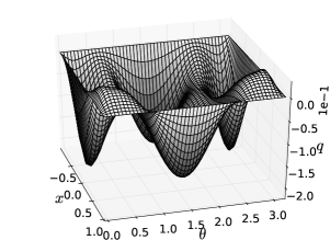
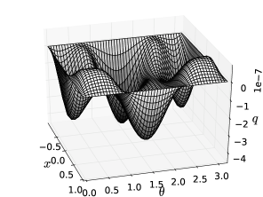
Figure 1: Numerical solutions. The numerical values of the function $q$ for the choice $m=2$, $d=10$, $r_{\mathrm{ext}}=2\,r_{\mathrm{int}}$, and $M$ according to Tab. 1 with the gluing annulus placed at (a) $r_{\mathrm{int}}=6$ and (b) $r_{\mathrm{int}}=500$. The values of $q$ decrease with the distance of the gluing annulus from the origin. The resolution used to produce the plots is $K=L=35$ collocation points.

The accuracy and convergence properties of the solutions presented in Fig. 1 are similar to the ones observed in [7]. Namely, the expansion coefficients in (8) decay to zero exponentially, and their actual values $a_{kl}$ for $k,l>60$ are of the order of $10^{-14}$ (numerical roundoff).

3.3 Behaviour of the ADM mass

Here, we will investigate any possible effects that the introduction of the gluing region has on the total ADM mass $M$ of our construction. One expects that the presence of the Brill wave in the gluing region would in general increase the overall ADM mass of the gluing construction. As was pointed out in [7], the positive mass theorem for time-symmetric, axisymmetric, vacuum gravitational waves proved by Brill [14] can be used in the form

$$M=\int^{\pi}_{0}\int^{\infty}_{0}\left[\left(\frac{1}{\psi}\frac{\partial\psi}{\partial r}\right)^{2}+\left(\frac{1}{r\,\psi}\frac{\partial\psi}{\partial\theta}\right)^{2}\right]r^{2}\sin\theta\,dr\,d\theta,$$ (10)

not only to determine the relation between the masses $m$ and $M$ involved in our construction, but also to study the behaviour of the ADM mass $M$ on the details of the gluing construction. In the expression above $\psi$ is the conformal factor defined by (4), thus the ADM mass $M$ enters also the right-hand side of (10). In the light of this observation, the relation (10) can be viewed as an integrability condition for the ADM mass in the following sense. For a specific choice of $M$, we compute numerically the integral quantity on the right-hand side of (10) and denote the result with $M_{I}$. We will be interested here in the cases that $M_{I}=M$ holds, as they correspond to true physical solutions. The case that $M_{I}$ takes values $M_{I}<2m$ corresponds to a reduction of the ADM mass, the case $M_{I}>2m$ to an increase.

In Tab. 1 a detailed study of the restrictions that the condition (10) poses on the ADM mass is presented for the choice $m=2$, $d=10$, $r_{\mathrm{ext}}=2\,r_{\mathrm{int}}$ of the free parameters that was used to generate the solutions of Fig. 1. The closer we place the gluing annulus to the origin, the greater is the increase of the ADM mass. The increase is limited only by the requirement that the gluing region lies outside of the horizons of the Brill-Lindquist data, i.e. $r_{\mathrm{int}}>d/2+m\,d/(2\,d+m)$. Notice that the actual increase of the ADM mass decreases extremely fast to zero with increasing gluing radius $r_{\mathrm{int}}$.

$r_{\mathrm{int}}$	$M_{I}$	$M_{I}-2m$	$|\Delta M|$	$\delta M$
6	4.08778	0.08778	$1.4\times 10^{-5}$	$1.5\times 10^{-5}$
10	4.0119	0.0119	$3.9\times 10^{-5}$	$4.5\times 10^{-5}$
30	4.00017185	0.00017185	$3.4\times 10^{-8}$	$7.9\times 10^{-8}$
100	4.00000145	$1.45\times 10^{-6}$	$1.6\times 10^{-8}$	$2.2\times 10^{-8}$
500	4.0000000024	$2.4\times 10^{-9}$	$3.3\times 10^{-11}$	$4\times 10^{-11}$

Table 1: Increase of the ADM mass. The increased ADM mass, the actual increase, the violation of the integrability condition $\Delta M=M_{I}-M$, and the numerical error $\delta M$ involved in these calculations are presented for different locations of the gluing annulus. Notice that by just quintupling the gluing radius (from 6 to 30), the increase decreases by two orders of magnitude.

In [7] it has been shown that for the $\theta$-independent gluing function

$$\beta(r)=\frac{1}{2}\left(1+\tanh\left(\frac{1}{r-r_{\mathrm{int}}}+\frac{1}{r-r_{\mathrm{ext}}}\right)\right),$$

it is possible to reduce the ADM mass in the rather extreme case that the black holes are placed very close to each other and the gluing is performed along a very wide gluing annulus that starts very close to the horizons of the black holes. Here, it was not possible to find a setup that could lead to a reduction of the ADM mass for the choice (5), even for such extreme configurations. It seems that even the simplest inclusion of $\theta$-dependence in the gluing function increases the contribution of the Brill wave to the ADM mass to a degree that makes it impossible to find an arrangement of our data that leads to reduction of the ADM mass.

4 Conclusions

In [7] we presented a numerical implementation of Corvino’s gluing method [1] applied to vacuum axisymmetric spacetimes [6]. Here, we focused on a gluing function with a simple $\theta$-dependence. It was shown numerically that for the choice (5), the vacuum time-symmetric constraint equations (6) admit smooth solutions that are of Schwarzschild type close to spatial infinity, see Fig. 1. We showed that these solutions converge exponentially and depend on the location of the gluing annulus in the expected way: the Brill wave function $q$ decreases with the distance of the gluing annulus from the origin. The latter observation confirms the expectation that in the limiting case that the gluing annulus is placed at infinity $q$ must tend to zero.

Our study of the dependence of the total ADM mass $M$ on the details of the gluing procedure carried out in Sec. 3.3 strongly indicates that for the choice (5) the presence of the gluing annulus tends always to increase the ADM mass. It seems that the Brill wave corresponding to (5) contributes to the overall ADM mass to such a degree that reduction was not possible, even in the extreme setup of [7] where a very wide gluing region starting close to the black hole horizons was chosen.

References

References

- [1] Corvino J 2000 Commun. Math. Phys. 214 137
- [2] Corvino J and Schoen R M 2006 J. Diff. Geom. 73 185 (Preprint gr–qc/0301071)
- [3] Cortier J 2013 Ann. Henri Poincaré 14 1109 (Preprint 1202.3688 [gr–qc])
- [4] Chruściel P T and Pollack D 2008 Ann. Henri Poincaré 9 639 (Preprint 0710.3365 [gr–qc])
- [5] Chruściel P T and Delay E 2009 Comm. Anal. Geom. 17 343 (Preprint 0711.1557 [gr–qc])
- [6] Giulini D and Holzegel G 2005 Corvino’s construction using Brill waves Preprint gr-qc/0508070
- [7] Doulis G and Rinne O 2014 Numerical construction of initial data for Einstein’s equations with static extension to space-like infinity Preprint 1411.7878 [gr-qc]
- [8] Chruściel P T and Delay E 2002 Class. Quantum Grav. 19 L71 (Preprint gr–qc/0203053)
- [9] Rinne O 2010 Class. Quantum Grav. 27 035014 (Preprint 0910.0139 [gr–qc])
- [10] Friedrich H 1998 J. Geom. Phys. 24 83
- [11] Beyer F, Doulis G, Frauendiener J and Whale B 2012 Class. Quantum Grav. 29 245013 (Preprint 1207.5854 [gr–qc])
- [12] Doulis G and Frauendiener J 2013 Gen. Relativ. Gravit. 454 1365 (Preprint 1301.4286 [gr–qc])
- [13] Brill D R and Lindquist R W 1963 Phys. Rev. 131 471
- [14] Brill D R 1959 Ann. Phys. 7 466