Negative interfacial tension in phase-separated active suspensions

Abstract

We study numerically a model for active suspensions of self-propelled repulsive particles, for which a stable phase separation into a dilute and a dense phase is observed. We exploit that for non-square boxes a stable “slab” configuration is reached, in which interfaces align with the shorter box edge. Evaluating a recent proposal for an intensive active swimming pressure, we demonstrate that the excess stress within the interface separating both phases is negative. The occurrence of a negative tension together with stable phase separation is a genuine non-equilibrium effect that is rationalized in terms of a positive stiffness, the estimate of which agrees excellently with the numerical data. Our results challenge effective thermodynamic descriptions and mappings of active suspensions onto passive pair potentials with attractions.

Equilibrium statistical physics Chandler (1987) rests on two deceptively simple premises: the laws of conservation and the uniform probability of all accessible microstates in isolated systems. Of course, suitable local equilibria are only a small part of the universe, and non-equilibrium encompasses so many diverse processes and phenomena that the quest for a universal description is one of the great challenges in statistical physics. While likely futile in full generality, there are subclasses of driven systems for which a comprehensive theory seems to be in reach. One such class are suspensions of active particles.

Active matter Romanczuk et al. (2012); Marchetti et al. (2013); Jens Elgeti (2014) has emerged as a paradigm to describe a broad wealth of non-equilibrium collective, dynamical behavior ranging from droplets Thutupalli et al. (2011) to bacteria Wensink et al. (2012) down to microtubule networks driven by molecular motors Sanchez et al. (2012). Here we focus on suspensions of self-propelled colloidal spherical particles suspended in a solvent (see Ref. 8 for a short perspective of these systems and references) or polymer solution Schwarz-Linek et al. (2012). Quite strikingly, particles cluster into dense and dilute regions for high enough density and swimming speeds. Such a behavior has been observed both experimentally Theurkauff et al. (2012); Palacci et al. (2013); Buttinoni et al. (2013) and in computer simulations of purely repulsive particles Bialké et al. (2013); Redner et al. (2013); Fily et al. (2014); Stenhammar et al. (2013, 2014); Wysocki et al. (2014); Takatori et al. (2014). It is understood microscopically to arise from the time-scale separation between the decorrelation time of the directed motion and the collision rate, which is controlled by speed and density. The actual time-scales depend on many details (pair potentials, swimming mechanisms, hydrodynamic interactions Zöttl and Stark (2014)) but the generic effect is robust and only requires volume exclusion in combination with a persistent motion of the particles.

Since the formation and growth of dense domains indeed resembles the phase separation of passive suspensions with attractive interactions, several theoretical descriptions following a “thermodynamical” route have been proposed: effective mean-field free energies Tailleur and Cates (2008); Speck et al. (2014); Cates and Tailleur (2014), pressure equations of state Wittkowski et al. (2014); Takatori et al. (2014); Takatori and Brady (2014); Ginot et al. (2014), and mappings to effective isotropic pair potentials Schwarz-Linek et al. (2012); Das et al. (2014). However, microscopic interactions of the self-propelled particles are not isotropic and the crucial physical ingredient, as mentioned, is the persistence of motion over a length $\ell_{\text{p}}=v_{0}\tau_{\text{r}}$, where $v_{0}$ is the swimming speed and $\tau_{\text{r}}$ the time over which orientations decorrelate. In this Letter, we numerically test the idea of an intensive pressure in active suspensions assuming an equation of state exists Solon et al. (2014). We adopt a strategy that has proven to be very fruitful in the study of phase-separated passive systems by exploiting finite-size transitions in non-square simulation boxes Schmitz et al. (2014). Following old ideas by Kirkwood and Buff Kirkwood and Buff (1949) together with a generalization of the swimming pressure Takatori et al. (2014) gives us access to the interface Evans (1979), and we show that the interfacial tension is actually negative. In contrast, the stiffness governing the interface fluctuations is positive, and we show how to relate both through the dissipated work.

We simulate a minimal model for active particles that has been studied by a range of groups Bialké et al. (2013); Redner et al. (2013); Fily et al. (2014); Stenhammar et al. (2013, 2014); Wysocki et al. (2014); Takatori et al. (2014). The model consists of $N$ particles with diameter $a$ interacting via short-ranged repulsive forces (here from a Weeks-Chandler-Andersen potential $u(r)$, for details and parameters see Refs. 12; 8). The dynamics is overdamped,

$$\dot{\mathbf{r}}_{i}=-\nabla_{i}U+v_{0}\mathbf{e}_{i}+\boldsymbol{\xi}_{i},$$ (1)

where $\boldsymbol{\xi}_{i}$ is the Gaussian translational noise with zero mean and correlations $\langle\boldsymbol{\xi}_{i}(t)\boldsymbol{\xi}_{j}^{T}(t)\rangle=2\delta_{ij}\mathbf{1}\delta(t-t^{\prime})$, and $U=\sum_{j<i}u(|\mathbf{r}_{i}-\mathbf{r}_{j}|)$ is the total potential energy. We consider the two dimensional case with a simulation box of size $L_{x}\times L_{y}$ employing either periodic boundary conditions, or walls in the $x$ direction and periodic boundaries in the $y$ direction. Every particle swims with fixed speed $v_{0}$ along its unity orientation $\mathbf{e}_{i}$, which undergoes free rotational diffusion with diffusion coefficient $1/\tau_{\text{r}}$. We employ dimensionless quantities such that lengths are measured in units of $a$ and time in units of $D_{0}/a^{2}$, where $D_{0}$ is the bare translational diffusion coefficient. The no-slip boundary condition then implies $\tau_{\text{r}}=\tfrac{1}{3}$. Moreover, energies are measured in units of $k_{\text{B}}T$ for fixed solvent temperature $T$.

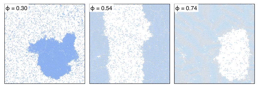
Figure 1: Finite-size transitions of active Brownian particles (in a box with aspect ratio 1.2) going from low to high density: droplet, slab, and bubble.

We first scan the system for swimming speed $v_{0}=180$ and vary the global density $\bar{\rho}=N/A$. As shown in Fig. 1, we observe finite-size transitions as we increase the density: from the homogeneous suspension to a droplet of the dense phase, to a slab, to a “bubble” (or void) forming within the dense phase. These transitions appear to be exact counterparts of the transitions observed in simulations of vapor-liquid coexistence in finite volumes Schrader et al. (2009). While the snapshots in Figs. 1 and 2(a) show a high degree of local order in the dense phase, these crystalline patches have only a short lifetime and constantly reorganize. Hence, particles do not freeze and the description as an active liquid-vapor coexistence is more appropriate.

To make comparisons with passive suspensions easier, densities will be reported as area fractions $\phi=\bar{\rho}\pi(a^{\ast}/2)^{2}$ using an effective hard-sphere diameter $a^{\ast}=0.984a$ obtained via Barker-Henderson from the pair potential Barker and Henderson (1967). Such a mapping is known to work well for passive repulsive suspensions although at high swimming speeds it will certainly become less reliable. In the following, we exploit the slab configuration and all simulations are run at $\phi=0.49$ with $N=10,000$ particles varying the speed $v_{0}$. In analogy to simulations of passive fluids, we employ a non-square box of area $A=L_{x}L_{y}$ with edge lengths $L_{x}>L_{y}$ such that the slab of the dense phase is encouraged to span the shorter length, see Fig. 2(a). At high enough swimming speeds $v_{0}$, such slabs form spontaneously and remain stable. In order to reach the steady state faster, all $N$ particles are initially placed in a dense slab in the middle of the system. After a relaxation time of $t_{\text{rel}}=100$ we start to collect and analyze data.

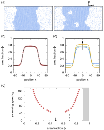
Figure 2: Slab geometry: (a) Snapshots of a phase separated system with aspect ratio $L_{x}/L_{y}=2$. A dense slab is surrounded by the dilute gas phase. Large fluctuations occur, not only at the interface but also the dense inner region of the slab might develop “holes” (right snapshot). (b) Measured density profile for $v_{0}=100$ (symbols) and fit of Eq. (2) (line). (c) Measured density profiles for $v_{0}=80,100,150$ (from bottom to top) from which we extract the coexisting densities. (d) Resulting phase diagram: The symbols show the coexisting densities $\phi_{\pm}$ with errors estimated from 5 independent runs (except $v_{0}=170$ with two runs). The dashed vertical line indicates the freezing area fraction $\phi\simeq 0.7$ and the shaded area the excluded packing fractions for real hard disks. The arrow indicates the global density $\phi=0.49$ at which simulations are run.

Qualitatively, looking at the simulations one notes that fluctuations are much more violent than expected from a passive suspension. In particular, even in the dense phase larger “bubbles” might form, see Fig. 2(a). Still, given sufficient statistics, the averaged density profiles excellently fit the mean-field functional form

$$\phi(x)=\frac{\phi_{+}+\phi_{-}}{2}+\frac{\phi_{+}-\phi_{-}}{2}\tanh\left(\frac{x-x_{0}}{2w}\right),$$ (2)

see Fig. 2(b). Here, $x_{0}$ marks the midpoint of the profile and $w$ is related to the width of the interface. Density profiles are measured from the simulations by dividing the simulation box into slices with area $A_{1}$, where $x$ is the distance of the slice from the center-of-mass. Although the two interfaces are correlated, in a first attempt we treat them independently and perform separate fits for $x<0$ and $x>0$. The interfacial width $w$ and bulk phase densities $\phi_{\pm}$ are then obtained by taking the mean of the results for the left and right half of the box. Measured density profiles for several speeds are shown in Fig. 2(c). For each profile, we fit Eq. (2) from which we extract the coexisting densities $\phi_{\pm}$ shown in Fig. 2(d). Note that the error increases as we go to lower speeds as expected from critical fluctuations.

We now study the mechanical stress generated in the active suspension. To this end, we focus on a single swimming speed $v_{0}=100$. Note that the system is translationally invariant in the $y$-direction since we have encouraged the slab to align that way. Clearly, phase separation and the occurrence of interfaces breaks the translational invariance in $x$-direction so that averaged quantities can only depend on $x$. The condition of hydrostatic equilibrium $\nabla\cdot\mathbf{p}=0$ then implies that the total pressure $\mathbf{p}(x)$ is a diagonal tensor and, moreover, that the normal pressure $p_{xx}=p_{\text{N}}$ is constant throughout the box to ensure mechanical stability. In contrast, the tangential pressure $p_{yy}(x)=p_{\text{T}}(x)$ can, and does, vary spatially with $x$.

We first consider the pressure tensor

$$\mathbf{p^{\text{(i)}}}(x)=\frac{1}{2A_{1}}\langle\mathbf{r}_{ij}\mathbf{f}_{ij}^{T}\rangle_{x}$$ (3)

due to particle interactions, where $\mathbf{r}_{ij}=\mathbf{r}_{i}-\mathbf{r}_{j}$ is the connecting vector of particles $i$ and $j$, and $\mathbf{f}_{ij}$ is the pair force along this vector due to the repulsive potential. The brackets $\langle\cdot\rangle_{x}$ denote the average over particle pairs for which at least one particle is within the slice at $x$. The factor $\tfrac{1}{2}$ has to be included to compensate for the fact that every bond crossing between slices is counted twice. Note that there are alternative spatial discretization schemes, all of which lead to the same integrated pressure Walton et al. (1983). The two diagonal components $p^{\text{(i)}}_{xx}$ and $p^{\text{(i)}}_{yy}$ are plotted in Fig. 3(a). Both curves lie on top of each other and follow qualitatively the density, i.e., the interaction pressure is low in the dilute phase and high in the dense phase. Clearly, there is something missing since such an inhomogeneous pressure is mechanically unstable and violates the condition of hydrostatic equilibrium.

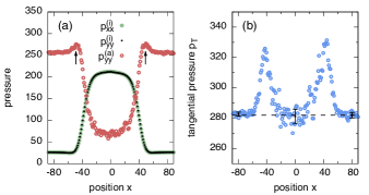
Figure 3: Pressure profiles for $v_{0}=100$: (a) The diagonal components $p^{\text{(i)}}_{xx}$ ($\bullet$) and $p^{\text{(i)}}_{yy}$ ($\cdot$) of the interaction pressure (which lie on top of each other) and the tangential active pressure $p^{\text{(a)}}_{yy}$ ($\circ$). Note the increase of the active pressure in the interface before it drops in the dense phase (arrows). (b) The total tangential pressure $p_{\text{T}}=\rho+p^{\text{(i)}}_{yy}+p^{\text{(a)}}_{yy}$. The dashed line is the estimate for the bulk pressure $p\simeq 282$, the error bars show the root-mean-square errors of local horizontal fits.

Only very recently, the idea that due to their directed motion the particles exert a mechanical stress has been formalized by Brady and coworkers Takatori et al. (2014). Following their approach, the scalar active pressure can be calculated via

$$p^{\text{(a)}}=\frac{v_{0}}{2A}\sum_{i=1}^{N}\langle\mathbf{e}_{i}\cdot\mathbf{r}_{i}\rangle,$$ (4)

where $\mathbf{r}_{i}$ is indeed the absolute position. The active pressure thus stems from the correlations between particle positions and orientations. Assuming a gas of non-interacting swimmers with $\dot{\mathbf{r}}_{i}=v_{0}\mathbf{e}_{i}+\boldsymbol{\xi}_{i}$, we obtain Takatori et al. (2014)

$$p^{\text{(a)}}_{\text{id}}=\frac{v_{0}}{2A}\sum_{i=1}^{N}\int_{-\infty}^{t}\mathrm{d}t^{\prime}\;\langle\mathbf{e}_{i}(t)\cdot\dot{\mathbf{r}}_{i}(t^{\prime})\rangle=\frac{1}{2}\bar{\rho}v_{0}^{2}\tau_{\text{r}}$$ (5)

using the correlation function $\langle\mathbf{e}(t)\cdot\mathbf{e}(t^{\prime})\rangle=e^{-|t-t^{\prime}|/\tau_{\text{r}}}$.

To consider the spatial dependence of the active pressure (4), we introduce the generalized tensor

$$\mathbf{p^{\text{(a)}}}(x)=\frac{v_{0}}{A_{1}}\langle\mathbf{e}_{i}\mathbf{r}_{i}^{T}\rangle_{x}$$ (6)

in analogy to Eq. (3). The average is now taken over the subset of particles that at time $t$ occupy slice $x$. However, there is a subtlety here since this destroys the correlations between the $x$-coordinate and the orientations, which, as Eq. (5) demonstrates, depend not only on the configuration but on the previous history. Hence, only the component $p^{\text{(a)}}_{yy}(x)$ is actually meaningful, which is plotted in Fig. 3(a). It again qualitatively follows the density but is now inverted with respect to the interaction pressure: the active pressure is high in the dilute region and drops considerably in the dense region. The physical reason is that particle motion is hindered in the dense phase and orientation and actual displacement are thus less correlated.

Two conceptual insights into the nature of active suspensions are gained by plotting the total tangential pressure $p_{\text{T}}(x)=\rho(x)+p^{\text{(i)}}_{yy}(x)+p^{\text{(a)}}_{yy}(x)$ (there is also the ideal gas contribution $\rho(x)$, which, however, is small). As demonstrated in Fig. 3(b), the bulk pressures of dense and dilute phase are equal, which in turn implies $p_{\text{N}}\approx p_{\text{T}}$. To corroborate that normal and tangential bulk pressure coincide, we have studied walls allowing to directly measure $p_{\text{N}}$ as the mechanical pressure exerted onto the walls [SM]. The first insight is thus that the swimming pressure of Takatori et al. is indeed the missing link to define and measure a pressure that is intensive. What is quite striking is that the pressure within the interface is larger than the bulk pressure. Identifying the interfacial tension with the excess stress (the factor $\tfrac{1}{2}$ again accounts for the two interfaces) leads to Kirkwood and Buff (1949)

$$\gamma=\frac{1}{2}\int_{0}^{L_{x}}\mathrm{d}x\;[p_{\text{N}}-p_{\text{T}}(x)]\simeq-842,$$ (7)

which becomes negative. This is the second, quite surprising insight. While it has no consequence for the mechanical stability, our intuition tells us that a system with a negative tension cannot be stable. The reason is that in systems for which classical thermodynamics is applicable, the interfacial tension determines the excess free energy due to the presence of interfaces. A negative tension implies that the suspension could lower its free energy by creating more interfaces, leading again to a homogeneous state. Quite in contrast, in active suspensions one observes a stable, phase-separated state.

Note that the excess stress is entirely due to the active pressure since $p^{\text{(i)}}_{xx}=p^{\text{(i)}}_{yy}$, which means in particular that there is no energetic contribution from the potential energy. Indeed, in Fig. 3(a) we observe an increase of the swimming pressure entering the interface before it drops. This can be understood qualitatively: the instantaneous interface has a small width [cf. snapshots Fig. 2(a)] and acts like a (flexible) wall. Swimmers accumulate but are still (comparably) free to slide along the interface in the $y$ direction, and hence their larger density (with respect to the dilute region) leads to a higher active tangential pressure $p^{\text{(a)}}_{yy}$. Another puzzling observation is the magnitude of $|\gamma|$, which is huge compared to typical values $\sim 1$ in passive liquids (e.g., for vapor-liquid coexistence in the Lennard-Jones fluid in two dimensions $\gamma_{\text{LJ}}\simeq 0.42$ has been reported Santra et al. (2008)).

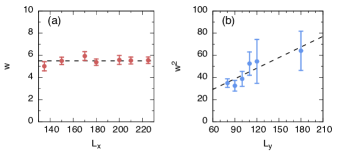
Figure 4: Interfacial width $w$ for $v_{0}=100$: (a) As a function of box length $L_{x}$ for constant $L_{y}=90$. The dashed line is a constant fit. (b) As a function of $L_{y}$ for constant $L_{x}=200$. The dashed line is a fit of Eq. (10) with $w_{0}\simeq 3.18$ and $\kappa\simeq 0.26$. Error bars show standard deviation of 10 independent runs.

To reach a better understanding, we now study the interfacial width $w$ in more detail. Fig. 4 shows $w$ obtained from several simulation runs at speed $v_{0}=100$ through fitting Eq. (2). We systematically study different system sizes by holding one box length fixed and varying the other. The total number of particles varies such that the global density is kept constant for all data points. While changing $L_{x}$ does not influence the width, we observe an increase of $w$ when increasing $L_{y}$. This behavior demonstrates two things: First, the system sizes considered here are large enough to have reached a constant width as we vary $L_{x}$. Second, the dependance on $L_{y}$ agrees with standard capillary wave theory (CWT) assuming equipartition. Hence, it is instructive to recall the arguments leading to CWT Evans (1979): One assumes an ideal instantaneous interface, in our case a line of total length $\ell$, which separates the two phases. To change this length, work has to be spent against the positive line tension. Assuming no overhangs, one can decompose the profile $h(y)=\sum_{q}h_{q}e^{\text{i}qy}$ into Fourier modes $h_{q}$. Since the energy for every mode stems from the thermal environment, equipartition implies $\langle|h_{q}|^{2}\rangle=(L_{y}\kappa q^{2})^{-1}$, where $\kappa$ is the interfacial stiffness governing the fluctuations. For passive liquid-vapor coexistence, this stiffness is equal to the tension (in units of $k_{\text{B}}T$ per unit length).

To estimate the interfacial width $w$, we calculate the fluctuations of the instantaneous interface [SM],

$$w^{2}\approx\sum_{q}\langle|h_{q}|^{2}\rangle=w_{0}^{2}+\frac{L_{y}}{12\kappa},$$ (8)

which predict a linear divergence due to the capillary waves. The offset $w_{0}^{2}$ corresponds to fluctuations of the $q=0$ mode, which are bounded due to the periodic boundary conditions. Moreover, we have assumed that even in the driven active suspension equipartition holds. While the use of equipartition is of course not rigorous, the predicted leading linear dependence on $L_{y}$ agrees quite well with the simulation data in Fig. 4(b). It can be further motivated by the fact that orientational degrees of freedom do not develop long-ranged correlations (even in the phase-separated case). Using Eq. (10) we can thus fit the data in Fig. 4(b) to extract the stiffness $\kappa\simeq 0.26$, which is both positive and small. That it is positive agrees with the observation of stable phase separation and finite-size transitions, that it is small agrees qualitatively with the observed strong fluctuations.

Finally, to rationalize a positive stiffness with a negative tension, recall that every particle swims with fixed velocity $v_{0}$, i.e., from the particle’s perspective it pumps the surrounding fluid against its own hydrodynamic drag. Hence, the particles constantly spent a “housekeeping” work $\mathcal{W}<0$ on the solvent. The typical scale of this work per particle is the hydrodynamic force times the persistence length, $\mathcal{W}/N=-v_{0}\ell_{\text{p}}=-v_{0}^{2}\tau_{\text{r}}$ (in Ref. 25 this expression appears as a positive energy scale). As long as the work per length $\gamma$ gained from extending the interface is smaller, the interface is stable. The housekeeping work thus fulfills a role similar to the thermal energy in passive suspension. For the stiffness we then find $\kappa\approx\gamma/(-v_{0}\ell_{\text{p}})\simeq 0.25$ for $v_{0}=100$, which compares favorably with the value extracted from the fitted interfacial widths.

In summary, we have demonstrated that the mechanical interfacial tension in phase-separated active suspensions is negative. This implies that work is released when the interfacial length $\ell$ is increased. However, this work is not “available” to the suspension but part of the work that is spent by the particles to drive the surrounding fluid. We expect that a negative tension is not specific to the model studied here but holds more generally in active matter. In principle, it can be observed in particle-resolved experiments Theurkauff et al. (2012); Palacci et al. (2013); Buttinoni et al. (2013) with a stabilized interface. The incorporation of both a negative tension and correct interfacial fluctuations into thermodynamic descriptions based on an effective free energy, a concept that seems to work well for the bulk phases Cates and Tailleur (2014); Takatori and Brady (2014), is certainly challenging. The deeper reason is that in thermal equilibrium the same free energy determines the probability of fluctuations away from typical configurations, a connection that no longer holds for systems driven away from thermal equilibrium.

I Interface fluctuations

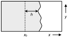
Figure 5: Sketch of the instantaneous interface, where $h(y)$ is the distance from the midpoint $x_{0}$ of the averaged profile.

For completeness, here we provide more detailed informations regarding the determination of the interface fluctuations. We consider a single interface with midpoint $x_{0}=0$ and we assume that we could determine an instantaneous interface in form of a line such that $h(y)$ denotes the position as a function of $y$, see Fig. 5. We decompose the profile into Fourier modes

$$h(y)=\sum_{q}h_{q}e^{\text{i}qy}\quad\text{with}\quad h_{q}=\frac{1}{L_{y}}\int_{0}^{L_{y}}\mathrm{d}y\;h(y)e^{-\text{i}qy}$$

and determine the interfacial width due to fluctuations through

$$w^{2}=\frac{1}{L_{y}}\int_{0}^{L_{y}}\mathrm{d}y\;\langle[h(y)]^{2}\rangle=\sum_{q}\langle|h_{q}|^{2}\rangle.$$ (9)

I.1 Equipartition

In passive suspensions in thermal equilibrium, the excess (free) energy due to the interface is $E_{\text{s}}=\gamma\ell$, where $\gamma$ is the interfacial tension and $\ell$ is the length of the interface. Expanding to lowest order in the gradient, one finds

$$\ell=\int_{0}^{L_{y}}\mathrm{d}y\;\sqrt{1+[h^{\prime}(y)]^{2}}\approx L_{y}+\frac{1}{2}L_{y}\sum_{q}q^{2}|h_{q}|^{2}$$

which is quadratic in the Fourier coefficients. Hence, equipartition implies

$$\langle|h_{q}|^{2}\rangle=\frac{1}{\kappa L_{y}q^{2}}$$

with $\kappa=\gamma$. Plugging this relation back into Eq. (9), we obtain

$$w^{2}=w_{0}^{2}+\frac{2}{\kappa L_{y}}\sum_{q>0}\frac{1}{q^{2}}=w_{0}^{2}+\frac{L_{y}}{12\kappa},$$ (10)

where $w_{0}^{2}$ describes the fluctuations of the $q=0$ mode and the second term the contribution due to the undulations (capillary waves) of the interface line. For this result we have employed $q=\frac{2\pi}{L_{y}}n$ due to the periodic boundaries together with the sum

$$\sum_{n=1}^{\infty}\frac{1}{n^{2}}=\frac{\pi^{2}}{6}.$$

For the active suspension we assume that Eq. (10) still holds albeit now with a stiffness $\kappa\neq\gamma$.

I.2 Density profile

From the profile $h(y)$ we can construct the instantaneous density profile

$$\hat{\rho}(x)=\frac{1}{L_{y}}\int_{0}^{L_{y}}\mathrm{d}y\;\left[\rho_{+}\theta(x-h(y))+\rho_{-}\theta(h(y)-x)\right],$$

where $\theta(x)$ is the unit step (Heaviside) function. The derivative of the mean profile thus reads

$$\frac{\partial\langle\hat{\rho}\rangle}{\partial x}=(\rho_{+}-\rho_{-})\langle\delta(x-h(y))\rangle.$$

Due to translational invariance, the expectation value becomes independent of $y$. It can be calculated from the characteristic function

$$\langle e^{\text{i}kh}\rangle=\exp\left\{-2k^{2}\sum_{q>0}\frac{1}{\kappa L_{y}q^{2}}\right\}=e^{-k^{2}w^{2}}$$

again assuming equipartition. Performing the reverse transformation, we obtain

$$\frac{\partial\langle\hat{\rho}\rangle}{\partial x}\propto\frac{\rho_{+}-\rho_{-}}{w}\exp\left\{-\frac{x^{2}}{4w^{2}}\right\}$$

for the variation of the mean density profile.

In the main text, we have chosen to fit density profiles using the mean-field expression

$$\rho(x)=\frac{\rho_{+}+\rho_{-}}{2}+\frac{\rho_{+}-\rho_{-}}{2}\tanh\left(\frac{x}{2w}\right).$$ (11)

The spatial derivative reads

$$\frac{\partial\rho}{\partial x}=\frac{\rho_{+}-\rho_{-}}{2w}\operatorname{sech}^{2}\left(\frac{x}{2w}\right)\approx\frac{\rho_{+}-\rho_{-}}{2w}\exp\left\{-\frac{x^{2}}{4w^{2}}\right\},$$

where $\operatorname{sech}x=1/\cosh x$. For the final result, we have expanded $\ln\operatorname{sech}x\approx-x^{2}/2$ to second order. This demonstrates that we can estimate the width $w$ appearing in Eq. (11) using Eq. (10).

II Walls

Figure 6: Phase-separated active suspension in the presence of walls: (a) Snapshot and (b) density profile showing the strong layering close to the walls. (c) The different pressures as a function of $x$ (the distance from the box center). The arrows indicate the pressure exerted onto the walls measured independently for left and right wall, and the upper dashed line shows their mean value $\simeq 272$. The lower dashed line indicates zero pressure.

We have also studied the active suspension in the presence of walls in the $x$ direction. As shown in Fig. 6(a), the particles now accumulate close to the walls and leave a dilute region between. We again determine the density profile, however, now the absolute distance $x$ from the center of the simulation box is used. Although we now use $N=20,000$ particles to improve statistics, obtaining good data is far more difficult compared to periodic boundaries. The main reason is the strong layering of particles close to the wall, see Fig. 6(b).

The walls consist of a short-ranged potential. The advantage is that we can now determine the force exerted on the walls, and therefore the pressure $p_{\text{N}}$, directly. As demonstrated in Fig. 6(c), within errors we find the same value as expected for an intensive pressure. Moreover, it agrees with the sum of active and interaction pressure in the dilute region, $p_{\text{T}}\approx p_{\text{N}}$. Note that the interaction pressure in the dilute phase becomes close to zero, whereas the swimming pressure close to the walls (apparently) averages to zero as well.