A Perturbation of the Dunkl Harmonic Oscillator on the Line

A Perturbation of the Dunkl Harmonic Oscillator
on the Line

Jesús A. ÁLVAREZ LÓPEZ ^†, Manuel CALAZA ^‡ and Carlos FRANCO ^†

J.A. Álvarez López, M. Calaza and C. Franco

^† Departamento de Xeometría e Topoloxía, Facultade de Matemáticas,
^† Universidade de Santiago de Compostela, 15782 Santiago de Compostela, Spain jesus.alvarez@usc.es, carlosluis.franco@usc.es

^‡ Laboratorio de Investigación 2 and Rheumatology Unit,
^‡ Hospital Clinico Universitario de Santiago, Santiago de Compostela, Spain manuel.calaza@usc.es

Received February 19, 2015, in final form July 20, 2015; Published online July 25, 2015;
Corrected June 28, 2017

Let $J_{\sigma}$ be the Dunkl harmonic oscillator on ${\mathbb{R}}$ ($\sigma>-\frac{1}{2}$). For $0<u<1$ and $\xi>0$, it is proved that, if $\sigma>u-\frac{1}{2}$, then the operator $U=J_{\sigma}+\xi|x|^{-2u}$, with appropriate domain, is essentially self-adjoint in $L^{2}({\mathbb{R}},|x|^{2\sigma}dx)$, the Schwartz space ${\mathcal{S}}$ is a core of $\overline{U}^{1/2}$, and $\overline{U}$ has a discrete spectrum, which is estimated in terms of the spectrum of $\overline{J_{\sigma}}$. A generalization $J_{\sigma,\tau}$ of $J_{\sigma}$ is also considered by taking different parameters $\sigma$ and $\tau$ on even and odd functions. Then extensions of the above result are proved for $J_{\sigma,\tau}$, where the perturbation has an additional term involving, either the factor $x^{-1}$ on odd functions, or the factor $x$ on even functions. Versions of these results on ${\mathbb{R}}_{+}$ are derived.

Dunkl harmonic oscillator; perturbation theory

47A55; 47B25; 33C45

1 Introduction

The Dunkl operators on ${\mathbb{R}}^{n}$ were introduced by Dunkl [8, 9, 10], and gave rise to what is now called the Dunkl theory [25]. They play an important role in physics and stochastic processes (see, e.g., [13, 24, 27]). In particular, the Dunkl harmonic oscillators on ${\mathbb{R}}^{n}$ were studied in [11, 19, 20, 23]. We will consider only this operator on ${\mathbb{R}}$, where it is uniquely determined by one parameter. In this case, a conjugation of the Dunkl operator was previously introduced by Yang [28] (see also [21]).

Let us fix some notation that is used in the whole paper. Let ${\mathcal{S}}={\mathcal{S}}({\mathbb{R}})$ be the Schwartz space on ${\mathbb{R}}$, with its Fréchet topology. It decomposes as direct sum of subspaces of even and odd functions, ${\mathcal{S}}={\mathcal{S}}_{\text{\rm ev}}\oplus{\mathcal{S}}_{\text{\rm odd}}$. The even/odd component of a function in ${\mathcal{S}}$ is denoted with the subindex ev/odd. Since ${\mathcal{S}}_{\text{\rm odd}}=x{\mathcal{S}}_{\text{\rm ev}}$, where $x$ is the standard coordinate of ${\mathbb{R}}$, $x^{-1}\phi\in{\mathcal{S}}_{\text{\rm ev}}$ is defined for $\phi\in{\mathcal{S}}_{\text{\rm odd}}$. Let $L^{2}_{\sigma}=L^{2}({\mathbb{R}},|x|^{2\sigma}dx)$ ($\sigma\in{\mathbb{R}}$), whose scalar product and norm are denoted by $\langle\ ,\ \rangle_{\sigma}$ and $\|\ \|_{\sigma}$. The above decomposition of ${\mathcal{S}}$ extends to an orthogonal decomposition, $L^{2}_{\sigma}=L^{2}_{\sigma,\text{\rm ev}}\oplus L^{2}_{\sigma,\text{\rm odd}}$, because the function $|x|^{2\sigma}$ is even. ${\mathcal{S}}$ is a dense subspace of $L^{2}_{\sigma}$ if $\sigma>-\frac{1}{2}$, and ${\mathcal{S}}_{\text{\rm odd}}$ is a dense subspace of $L^{2}_{\tau,\text{\rm odd}}$ if $\tau>-\frac{3}{2}$. Unless otherwise stated, we assume $\sigma>-\frac{1}{2}$ and $\tau>-\frac{3}{2}$. The domain of a (densely defined) operator $P$ in a Hilbert space is denoted by ${\mathsf{D}}(P)$. If $P$ is closable, its closure is denoted by $\overline{P}$. The domain of a (densely defined) sesquilinear form ${\mathfrak{p}}$ in a Hilbert space is denoted by ${\mathsf{D}}({\mathfrak{p}})$. The quadratic form of ${\mathfrak{p}}$ is also denoted by ${\mathfrak{p}}$. If ${\mathfrak{p}}$ is closable, its closure is denoted by $\bar{\mathfrak{p}}$. For an operator in $L^{2}_{\sigma}$ preserving the above decomposition, its restrictions to $L^{2}_{\sigma,\text{\rm ev/odd}}$ will be indicated with the subindex ev/odd. The operator of multiplication by a continuous function $h$ in $L^{2}_{\sigma}$ is also denoted by $h$. The harmonic oscillator is the operator $H=-\frac{d^{2}}{dx^{2}}+s^{2}x^{2}$ ($s>0$) in $L^{2}_{0}$ with ${\mathsf{D}}(H)={\mathcal{S}}$.

The Dunkl operator on ${\mathbb{R}}$ is the operator $T$ in $L^{2}_{\sigma}$, with ${\mathsf{D}}(T)={\mathcal{S}}$, determined by $T=\frac{d}{dx}$ on ${\mathcal{S}}_{\text{\rm ev}}$ and $T=\frac{d}{dx}+2\sigma x^{-1}$ on ${\mathcal{S}}_{\text{\rm odd}}$, and the Dunkl harmonic oscillator on ${\mathbb{R}}$ is the operator $J=-T^{2}+s^{2}x^{2}$ in $L^{2}_{\sigma}$ with ${\mathsf{D}}(J)={\mathcal{S}}$. Thus $J$ preserves the above decomposition of ${\mathcal{S}}$, being $J_{\text{\rm ev}}=H-2\sigma x^{-1}\frac{d}{dx}$ and $J_{\text{\rm odd}}=H-2\sigma\frac{d}{dx}x^{-1}$. The subindex $\sigma$ is added to $J$ if needed. This $J$ is essentially self-adjoint, and the spectrum of $\overline{J}$ is well known [23]; in particular, $\overline{J}>0$. In fact, even for $\tau>-\frac{3}{2}$, the operator $J_{\tau,\text{\rm odd}}$ is defined in $L^{2}_{\tau,\text{\rm odd}}$ with ${\mathsf{D}}(J_{\tau,\text{\rm odd}})={\mathcal{S}}_{\text{\rm odd}}$ because it is a conjugation of $J_{\tau+1,\text{\rm ev}}$ by a unitary operator (Section 2). Some operators of the form $J+\xi x^{-2}$ ($\xi\in{\mathbb{R}}$) are conjugates of $J$ by powers $|x|^{a}$ ($a\in{\mathbb{R}}$), and therefore their study can be reduced to the case of $J$ [3]. Our first theorem analyzes a different perturbation of $J$.

Theorem 1.1.

Let $0<u<1$ and $\xi>0$. If $\sigma>u-\frac{1}{2}$, then there is a positive self-adjoint operator ${\mathcal{U}}$ in $L^{2}_{\sigma}$ satisfying the following:

• ${\mathcal{S}}$ is a core of ${\mathcal{U}}^{1/2}$, and, for all $\phi,\psi\in{\mathcal{S}}$,

  $$\big{\langle}{\mathcal{U}}^{1/2}\phi,{\mathcal{U}}^{1/2}\psi\big{\rangle}_{\sigma}=\langle J\phi,\psi\rangle_{\sigma}+\xi\big{\langle}|x|^{-u}\phi,|x|^{-u}\psi\big{\rangle}_{\sigma}.$$ (1.1)

• ${\mathcal{U}}$ has a discrete spectrum. Let $\lambda_{0}\leq\lambda_{1}\leq\cdots$ be its eigenvalues, repeated according to their multiplicity. There is some $D=D(\sigma,u)>0$, and, for each $\epsilon>0$, there is some $C=C(\epsilon,\sigma,u)>0$ so that, for all $k\in{\mathbb{N}}$,

  $$(2k+1+2\sigma)s+\xi Ds^{u}(k+1)^{-u}\leq\lambda_{k}\leq(2k+1+2\sigma)(s+\xi\epsilon s^{u})+\xi Cs^{u}.$$ (1.2)

Remark 1.2.

In Theorem 1.1, observe the following:

• The second term of the right hand side of (1.1) makes sense because $|x|^{-u}{\mathcal{S}}\subset L^{2}_{\sigma}$ since $\sigma>u-\frac{1}{2}$.

• ${\mathcal{U}}=\overline{U}$, where $U:=J+\xi|x|^{-2u}$ with ${\mathsf{D}}(U)=\bigcap_{m=0}^{\infty}{\mathsf{D}}({\mathcal{U}}^{m})$ (see [14, Chapter VI, Section 2.5]). The more explicit notation $U_{\sigma}$ will be also used if necessary.

• The restrictions ${\mathcal{U}}_{\text{ev/odd}}$ are self-adjoint in $L^{2}_{\sigma,\text{\rm ev/odd}}$ and satisfy (1.1) with $\phi,\psi\in{\mathcal{S}}_{\text{\rm ev/odd}}$ and (1.2) with $k$ even/odd. In fact, by the comments before the statement, ${\mathcal{U}}_{\tau,\text{odd}}$ is defined and satisfies these properties if $\tau>u-\frac{3}{2}$.

To prove Theorem 1.1, we consider the positive definite symmetric sesquilinear form ${\mathfrak{u}}$ defined by the right hand side of (1.1). Perturbation theory [14] is used to show that ${\mathfrak{u}}$ is closable and $\bar{\mathfrak{u}}$ induces a self-adjoint operator ${\mathcal{U}}$, and to relate the spectra of ${\mathcal{U}}$ and $\overline{J}$. Most of the work is devoted to check the conditions to apply this theory so that (1.2) follows; indeed, (1.2) is stronger than a general eigenvalue estimate given by that theory (Remark 3.22).

The following generalizations of Theorem 1.1 follow with a simple adaptation of the proof. If $\xi<0$, we only have to reverse the inequalities of (1.2). In (1.1), we may use a finite sum $\sum_{i}\xi_{i}\langle|x|^{-u_{i}}\phi,|x|^{-u_{i}}\psi\rangle_{\sigma}$, where $0<u_{i}<1$, $\sigma>u_{i}-\frac{1}{2}$ and $\xi_{i}>0$; then (1.2) would be modified by using $\max_{i}u_{i}$ and $\min_{i}\xi_{i}$ in the left hand side, and $\max_{i}\xi_{i}$ in the right hand side. In turn, this can be extended by taking ${\mathbb{R}}^{p}$-valued functions ($p\in{\mathbb{Z}}_{+}$), and a finite sum $\sum_{i}\langle|x|^{-u_{i}}\Xi_{i}\phi,|x|^{-u_{i}}\psi\rangle_{\sigma}$ in (1.1), where each $\Xi_{i}$ is a positive definite self-adjoint endomorphism of ${\mathbb{R}}^{p}$; then the minimum and maximum eigenvalues of all $\Xi_{i}$ would be used in (1.2).

As an open problem, we may ask for a version of Theorem 1.1 using Dunkl operators on ${\mathbb{R}}^{n}$, but we are interested in the following different type of extension. For $\sigma>-\frac{1}{2}$ and $\tau>-\frac{3}{2}$, let $L^{2}_{\sigma,\tau}=L^{2}_{\sigma,\text{\rm ev}}\oplus L^{2}_{\tau,\text{\rm odd}}$, whose scalar product and norm are denoted by $\langle\ ,\ \rangle_{\sigma,\tau}$ and $\|\ \|_{\sigma,\tau}$. Matrix expressions of operators refer to this decomposition. Let $J_{\sigma,\tau}=J_{\sigma,\text{\rm ev}}\oplus J_{\tau,\text{\rm odd}}$ in $L^{2}_{\sigma,\tau}$, with ${\mathsf{D}}(J_{\sigma,\tau})={\mathcal{S}}$. The hypotheses of the generalization of Theorem 1.1 are rather involved to cover enough cases of certain application that will be indicated.

Theorem 1.3.

Let $\xi>0$ and $\eta\in{\mathbb{R}}$, let

$$0<u<1,\qquad\sigma>u-\tfrac{1}{2},\qquad\tau>u-\tfrac{3}{2},\qquad\theta>-\tfrac{1}{2},$$ (1.3)

and set $v=\sigma+\tau-2\theta$. Suppose that the following conditions hold:

• If $\sigma=\theta\neq\tau$ and $\tau-\sigma\not\in-{\mathbb{N}}$, then

  $$\sigma-1<\tau<\sigma+1,2\sigma+\tfrac{1}{2}.$$ (1.4)

• If $\sigma\neq\theta=\tau$ and $\sigma-\tau\not\in-{\mathbb{N}}$, then

  $$-\tau,\tau-1<\sigma<3\tau+1,11\tau+2,\tau+1.$$ (1.5)

• If $\sigma\neq\theta=\tau+1$ and $\sigma-\tau-1\not\in-{\mathbb{N}}$, then

  $$\tau+1<\sigma<\tau+3,2\tau+\tfrac{7}{2}.$$ (1.6)

• If $\sigma\neq\theta\neq\tau$ and $\sigma-\theta,\tau-\theta\not\in-{\mathbb{N}}$, then

  $$\begin{split}&\tfrac{\sigma-\tau}{2}-1,\tfrac{\tau-\sigma}{2},\tfrac{\sigma+\tau-1}{4},\tfrac{\sigma+3\tau-2}{14},\tfrac{3\sigma+\tau-4}{14},\tfrac{\sigma+\tau-1}{2}<\theta<\tfrac{\sigma+\tau+1}{2},\\ &\tau-1<\sigma<\tau+3.\end{split}$$ (1.7)

Then there is a positive self-adjoint operator ${\mathcal{V}}$ in $L^{2}_{\sigma,\tau}$ satisfying the following:

• ${\mathcal{S}}$ is a core of ${\mathcal{V}}^{1/2}$, and, for all $\phi,\psi\in{\mathcal{S}}$,

  $$\big{\langle}{\mathcal{V}}^{1/2}\phi,{\mathcal{V}}^{1/2}\psi\big{\rangle}_{\sigma,\tau}=\langle J_{\sigma,\tau}\phi,\psi\rangle_{\sigma,\tau}+\xi\big{\langle}|x|^{-u}\phi,|x|^{-u}\psi\big{\rangle}_{\sigma,\tau}$$

  $$\hphantom{\big{\langle}{\mathcal{V}}^{1/2}\phi,{\mathcal{V}}^{1/2}\psi\big{\rangle}_{\sigma,\tau}=}{}+\eta\big{(}\big{\langle}x^{-1}\phi_{\text{\rm odd}},\psi_{\text{\rm ev}}\big{\rangle}_{\theta}+\big{\langle}\phi_{\text{\rm ev}},x^{-1}\psi_{\text{\rm odd}}\big{\rangle}_{\theta}\big{)}.$$ (1.8)

• Let $\varsigma_{k}=\sigma$ if $k$ is even, and $\varsigma_{k}=\tau$ if $k$ is odd. ${\mathcal{V}}$ has a discrete spectrum. Its eigenvalues form two groups, $\lambda_{0}\leq\lambda_{2}\leq\cdots$ and $\lambda_{1}\leq\lambda_{3}\leq\cdots$, repeated according to their multiplicity, such that there is some $D=D(\sigma,\tau,u)>0$ and, for every $\epsilon>0$, there are some $C=C(\epsilon,\sigma,\tau,u)>0$ and $E=E(\epsilon,\sigma,\tau,\theta)>0$ so that, for all $k\in{\mathbb{N}}$,

  $$\lambda_{k}\geq(2k+1+2\varsigma_{k})\big{(}s-2|\eta|\epsilon s^{\frac{v+1}{2}}\big{)}+\xi Ds^{u}(k+1)^{-u}-2|\eta|Es^{\frac{v+1}{2}},$$ (1.9)

  $$\lambda_{k}\leq(2k+1+2\varsigma_{k})\big{(}s+\epsilon\big{(}\xi s^{u}+2|\eta|s^{\frac{v+1}{2}}\big{)}\big{)}+\xi Cs^{u}+2|\eta|Es^{\frac{v+1}{2}}.$$ (1.10)

• Let $\tilde{u}\in{\mathbb{R}}$ such that

  $$0,v,\tau-2\theta+\tfrac{1}{2},\sigma-2\theta-\tfrac{1}{2}<\tilde{u}<1,v+1,\sigma+\tfrac{1}{2},\tau+\tfrac{3}{2},$$ (1.11)

  and let $\hat{u}=\max\{\tilde{u},v+1-\tilde{u}\}$. There is some $D=D(\sigma,\tau,u)>0$ and, for any $\epsilon>0$, there is some $\widetilde{C}=\widetilde{C}(\epsilon,\sigma,\tau,u)>0$ so that, for all $k\in{\mathbb{N}}$,

  $$\lambda_{k}\geq(2k+1+2\varsigma_{k})\big{(}s-|\eta|\epsilon s^{\hat{u}}\big{)}+\xi Ds^{u}(k+1)^{-u}-|\eta|\widetilde{C}s^{\hat{u}}.$$ (1.12)

• If $u=\frac{v+1}{2}$ and $\xi\geq|\eta|$, then there is some $\widetilde{D}=\widetilde{D}(\sigma,\tau,u)>0$ so that, for all $k\in{\mathbb{N}}$,

  $$\lambda_{k}\geq(2k+1+2\varsigma_{k})s+(\xi-|\eta|)\widetilde{D}s^{u}(k+1)^{-u}.$$ (1.13)

• If we add the term $\xi^{\prime}\langle\phi_{\text{\rm ev}},\psi_{\text{\rm ev}}\rangle_{\sigma}+\xi^{\prime\prime}\langle\phi_{\text{\rm odd}},\psi_{\text{\rm odd}}\rangle_{\tau}$ to the right hand side of (1.8), for some $\xi^{\prime},\xi^{\prime\prime}\in{\mathbb{R}}$, then the result holds as well with the additional term $\max\{\xi^{\prime},\xi^{\prime\prime}\}$ in the right hand side of (1.10), and the additional term, $\xi^{\prime}$ for $k\in 2{\mathbb{N}}$ and $\xi^{\prime\prime}$ for $k\in 2{\mathbb{N}}+1$, in the right hand sides of (1.9), (1.12) and (1.13).

Remark 1.4.

Note the following in Theorem 1.3:

• Like in Remark 1.2(ii), we have ${\mathcal{V}}=\overline{V}$, where

  $$V=\begin{pmatrix}U_{\sigma,\text{\rm ev}}&\eta|x|^{2(\theta-\sigma)}x^{-1}\\ \eta|x|^{2(\theta-\tau)}x^{-1}&U_{\tau,\text{\rm odd}}\end{pmatrix},$$

  with ${\mathsf{D}}(V)=\bigcap_{m=0}^{\infty}{\mathsf{D}}({\mathcal{V}}^{m})$. Note that the adjoint of $|x|^{2(\theta-\sigma)}x^{-1}\colon{\mathcal{S}}_{\text{\rm odd}}\to|x|^{2(\theta-\sigma)}{\mathcal{S}}_{\text{\rm ev}}$, as a densely defined operator of $L^{2}_{\tau,\text{\rm odd}}$ to $L^{2}_{\sigma,\text{\rm ev}}$, is given by $|x|^{2(\theta-\tau)}x^{-1}$, with the appropriate domain.

• Taking $\theta^{\prime}=\theta-1>-\frac{3}{2}$, since

  $$\langle x\phi,\psi\rangle_{\theta^{\prime}}=\big{\langle}\phi,x^{-1}\psi\big{\rangle}_{\theta}$$

  for all $\phi\in{\mathcal{S}}_{\text{\rm ev}}$ and $\psi\in{\mathcal{S}}_{\text{\rm odd}}$, we can write (1.8) as

  $$\big{\langle}{\mathcal{V}}^{1/2}\phi,{\mathcal{V}}^{1/2}\psi\big{\rangle}_{\sigma,\tau}=\langle J_{\sigma,\tau}\phi,\psi\rangle_{\sigma,\tau}+\xi\big{\langle}|x|^{-u}\phi,|x|^{-u}\psi\big{\rangle}_{\sigma,\tau}$$

  $$\hphantom{\big{\langle}{\mathcal{V}}^{1/2}\phi,{\mathcal{V}}^{1/2}\psi\big{\rangle}_{\sigma,\tau}=}{}+\eta\big{(}\langle\phi_{\text{\rm odd}},x\psi_{\text{\rm ev}}\rangle_{\theta^{\prime}}+\langle x\phi_{\text{\rm ev}},\psi_{\text{\rm odd}}\rangle_{\theta^{\prime}}\big{)}$$

  for all $\phi,\psi\in{\mathcal{S}}$, and, correspondingly,

  $$V=\begin{pmatrix}U_{\sigma,\text{\rm ev}}&\eta|x|^{2(\theta^{\prime}-\sigma)}x\\ \eta|x|^{2(\theta^{\prime}-\tau)}x&U_{\tau,\text{\rm odd}}\end{pmatrix}.$$

• The conditions (1.4), (1.5) and (1.6) describe three convex open subsets of ${\mathbb{R}}^{2}$ (Fig. 1). The condition (1.7) describes a convex open subset of ${\mathbb{R}}^{3}$ (Fig. 2), which is symmetric with respect to the plane defined by $\sigma=\tau+1$. It is a “semi-infinite bar” with 4 lateral faces, and 5 faces at the “bounded end.”

• In Theorem 1.3(iii), the condition (1.11) means that (1.3) also holds with $\tilde{u}$ and $v+1-\tilde{u}$ instead of $u$. There exists $\tilde{u}$ satisfying (1.11) just when

  $$0,v,\tau-2\theta+\tfrac{1}{2},\sigma-2\theta-\tfrac{1}{2}<1,v+1,\sigma+\tfrac{1}{2},\tau+\tfrac{3}{2}.$$ (1.14)

  This property is satisfied in the cases (b) and (d) by (1.3), (1.5) and (1.7); in particular, we can take $\tilde{u}=\frac{v+1}{2}$. In the case (a), if $\tau<3\sigma$, then (1.14) holds by (1.3) and (1.4). In the case (c), if $\sigma<3\tau+4$, then (1.14) holds by (1.3) and (1.6).

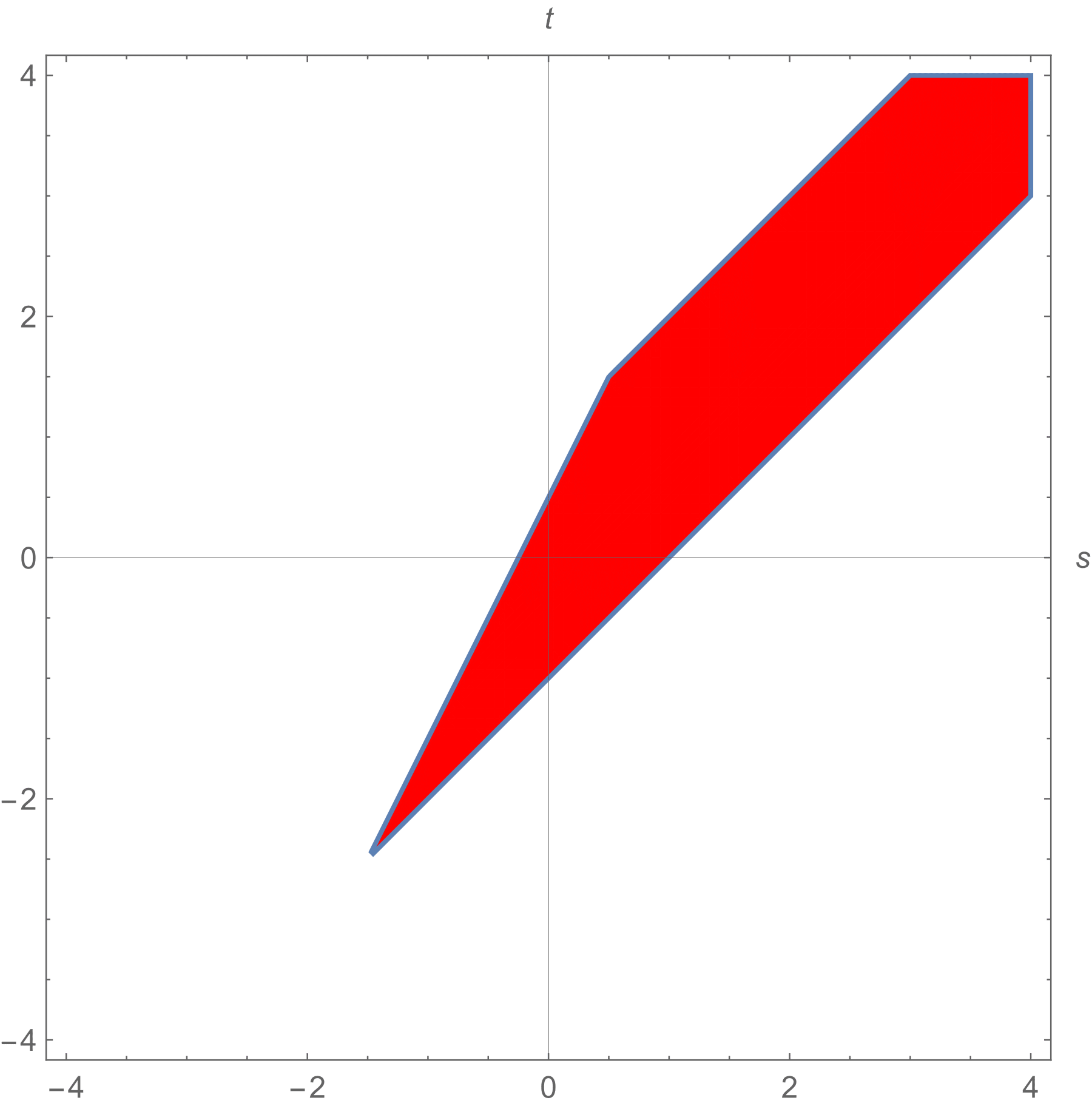
(a) Set defined by (1.4).

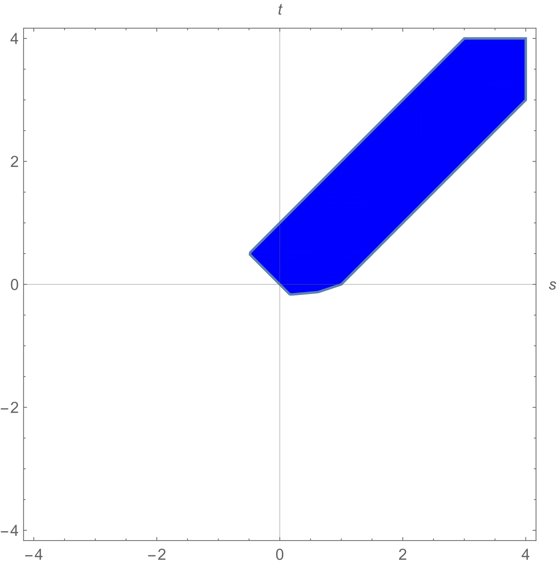
(b) Set defined by (1.5).

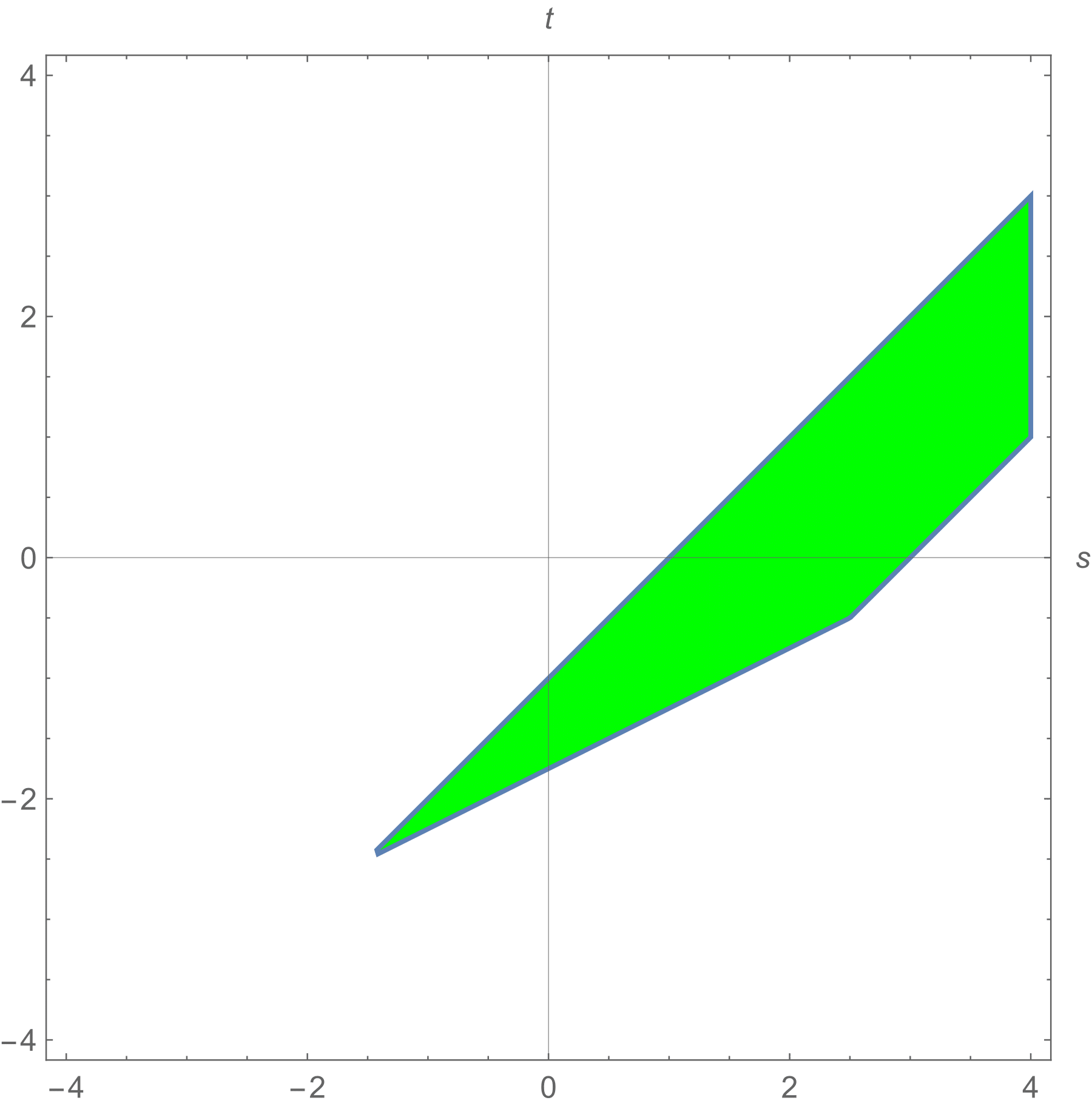
(c) Set defined by (1.6).

Figure 1: Sets in Theorem 1.3(a),(b),(c).

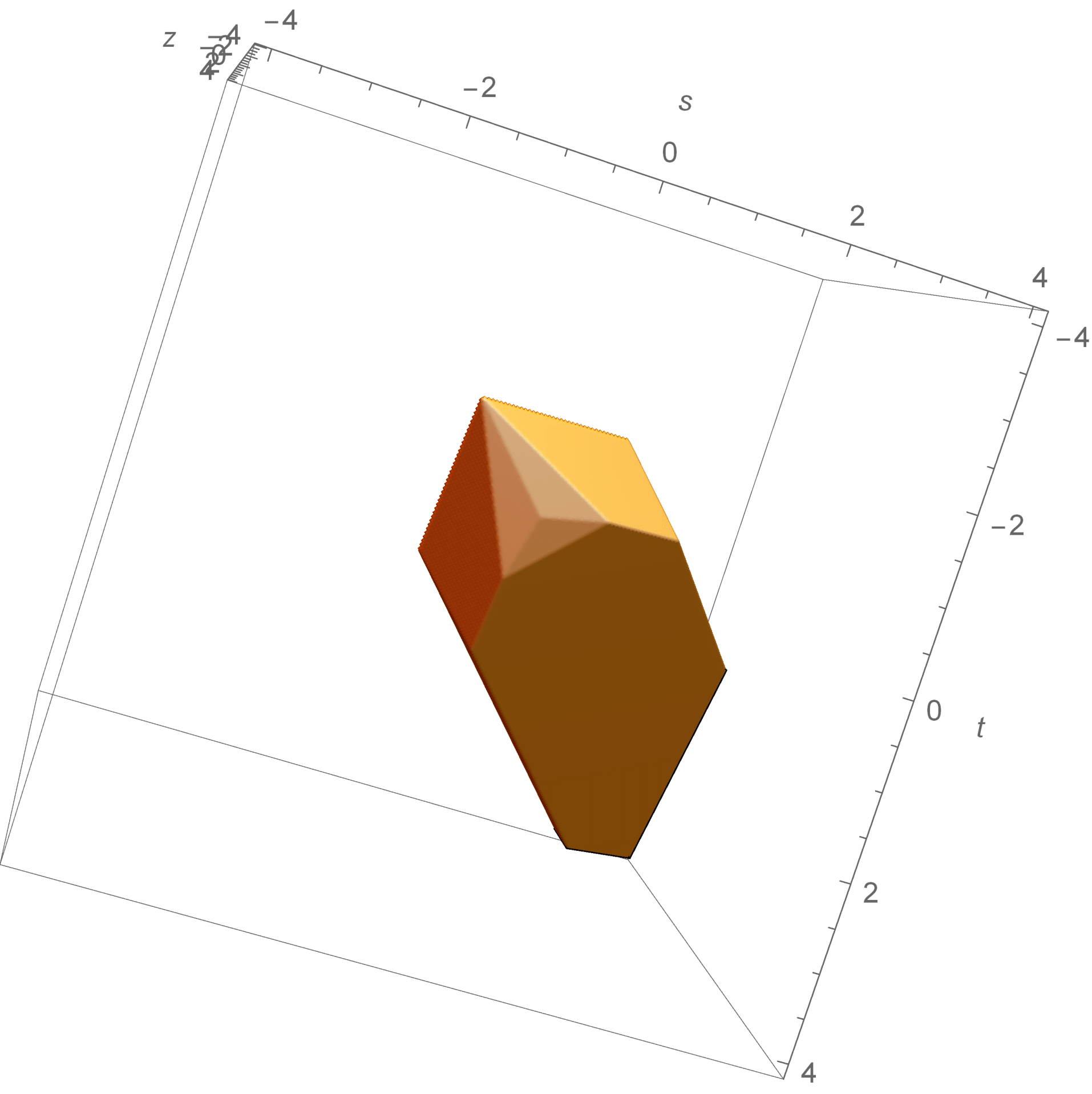
Figure 2: Set defined by (1.7) in Theorem 1.3(d).

The main arguments of the proofs of Theorems 1.1 and 1.3 are given in Sections 3–5. But some needed estimates are postponed to Sections 6 and 7 because they are of rather independent nature, and with rather long and tedious proofs.

Versions of these results on ${\mathbb{R}}_{+}$ are also derived in Section 8 (Corollaries 8.1, 8.2 and 8.3). In [4], these corollaries are used to study a version of the Witten’s perturbation $\Delta_{s}$ of the Laplacian on strata with the general adapted metrics of [6, 17, 18]. This gives rise to an analytic proof of Morse inequalities in strata involving intersection homology of arbitrary perversity, which was our original motivation. The simplest case of adapted metrics, corresponding to the lower middle perversity, was treated in [2] using an operator induced by $J$ on ${\mathbb{R}}_{+}$. The perturbations of $J$ studied here show up in the local models of $\Delta_{s}$ when general adapted metrics are considered. Some details of this application are given in Section 9.

2 Preliminaries

The Dunkl annihilation and creation operators are $B=sx+T$ and $B^{\prime}=sx-T$ ($s>0$). Like $J$, the operators $B$ and $B^{\prime}$ are considered in $L^{2}_{\sigma}$ with domain ${\mathcal{S}}$. They are perturbations of the usual annihilation and creation operators. The operators $T$, $B$, $B^{\prime}$ and $J$ are continuous on ${\mathcal{S}}$. The following properties hold [3, 23]:

• $B^{\prime}$ is adjoint of $B$, and $J$ is essentially self-adjoint.

• The spectrum of $\overline{J}$ consists of the eigenvalues $(2k+1+2\sigma)s$, $k\in{\mathbb{N}}$, of multiplicity one.

• The corresponding normalized eigenfunctions $\phi_{k}$ are inductively defined by

  $$\phi_{0}=s^{(2\sigma+1)/4}\Gamma\big{(}\sigma+\tfrac{1}{2}\big{)}^{-\frac{1}{2}}e^{-sx^{2}/2},$$ (2.1)

  $$\phi_{k}=\begin{cases}(2ks)^{-\frac{1}{2}}B^{\prime}\phi_{k-1}&\text{if $k$ is even},\\ (2(k+2\sigma)s)^{-\frac{1}{2}}B^{\prime}\phi_{k-1}&\text{if $k$ is odd},\end{cases}\qquad k\geq 1.$$ (2.2)

• The eigenfunctions $\phi_{k}$ also satisfy

  $$B\phi_{0}=0,$$ (2.3)

  $$B\phi_{k}=\begin{cases}(2ks)^{\frac{1}{2}}\phi_{k-1}&\text{if $k$ is even},\\ (2(k+2\sigma)s)^{\frac{1}{2}}\phi_{k-1}&\text{if $k$ is odd},\end{cases}\qquad k\geq 1.$$ (2.4)

• $\bigcap_{m=0}^{\infty}{\mathsf{D}}\big{(}\overline{J}^{m}\big{)}={\mathcal{S}}$.

By (2.1) and (2.2), we get $\phi_{k}=p_{k}e^{-sx^{2}/2}$, where $p_{k}$ is the sequence of polynomials inductively given by $p_{0}=s^{(2\sigma+1)/4}\Gamma(\sigma+\frac{1}{2})^{-\frac{1}{2}}$ and

$$p_{k}=\begin{cases}(2ks)^{-\frac{1}{2}}(2sxp_{k-1}-Tp_{k-1})&\text{if $k$ is even},\\ (2(k+2\sigma)s)^{-\frac{1}{2}}(2sxp_{k-1}-Tp_{k-1})&\text{if $k$ is odd},\end{cases}\qquad k\geq 1.$$

Up to normalization, $p_{k}$ is the sequence of generalized Hermite polynomials [26, p. 380, Problem 25], and $\phi_{k}$ is the sequence of generalized Hermite functions. Each $p_{k}$ is of degree $k$, even/odd if $k$ is even/odd, and with positive leading coefficient. They satisfy the recursion formula [3, equation (13)]

$$p_{k}=\begin{cases}k^{-\frac{1}{2}}\big{(}(2s)^{\frac{1}{2}}xp_{k-1}-(k-1+2\sigma)^{\frac{1}{2}}p_{k-2}\big{)}&\text{if $k$ is even},\\ (k+2\sigma)^{-\frac{1}{2}}\big{(}(2s)^{\frac{1}{2}}xp_{k-1}-(k-1)^{\frac{1}{2}}p_{k-2}\big{)}&\text{if $k$ is odd}.\end{cases}$$ (2.5)

When $k=2m+1$ ($m\in{\mathbb{N}}$), we have [3, equation (14)]

$$x^{-1}p_{k}=\sum_{i=0}^{m}(-1)^{m-i}\sqrt{\frac{m!\Gamma(i+\frac{1}{2}+\sigma)s}{i!\Gamma(m+\frac{3}{2}+\sigma)}}p_{2i}.$$ (2.6)

The Pochhammer symbol could be used to simplify this expression, as well as many other expressions in Sections 3 and 4. However there are quotients of gamma functions in Sections 4 and 5 that can not be simplified in this way (see e.g. Proposition 4.7). Thus, for the sake of uniformity, we use gamma functions in all quotients of this type.

Let ${\mathfrak{j}}$ be the positive definite symmetric sesquilinear form in $L^{2}_{\sigma}$, with ${\mathsf{D}}({\mathfrak{j}})={\mathcal{S}}$, given by ${\mathfrak{j}}(\phi,\psi)=\langle J\phi,\psi\rangle_{\sigma}$. Like in the case of $J$, the subindex $\sigma$ will be added to the notation $T$, $B$, $B^{\prime}$ and $\phi_{k}$ and ${\mathfrak{j}}$ if necessary. Observe that

$$B_{\sigma}=\begin{cases}B_{\tau}&\text{on ${\mathcal{S}}_{\text{\rm ev}}$},\\ B_{\tau}+2(\sigma-\tau)x^{-1}&\text{on ${\mathcal{S}}_{\text{\rm odd}}$},\end{cases}$$ (2.7)

$$B^{\prime}_{\sigma}=\begin{cases}B^{\prime}_{\tau}&\text{on ${\mathcal{S}}_{\text{\rm ev}}$},\\ B^{\prime}_{\tau}+2(\tau-\sigma)x^{-1}&\text{on ${\mathcal{S}}_{\text{\rm odd}}$}.\end{cases}$$ (2.8)

The operator $x\colon{\mathcal{S}}_{\text{\rm ev}}\to{\mathcal{S}}_{\text{\rm odd}}$ is a homeomorphism [3], which extends to a unitary operator $x\colon L^{2}_{\sigma,\text{\rm ev}}\to L^{2}_{\sigma-1,\text{\rm odd}}$. We get $xJ_{\sigma,\text{\rm ev}}x^{-1}=J_{\sigma-1,\text{\rm odd}}$ because $x\big{[}\frac{d^{2}}{dx^{2}},x^{-1}\big{]}=-2\frac{d}{dx}x^{-1}$. Thus, even for any $\tau>-\frac{3}{2}$, the operator $J_{\tau,\text{\rm odd}}$ is densely defined in $L^{2}_{\tau,\text{\rm odd}}$, with ${\mathsf{D}}(J_{\tau,\text{\rm odd}})={\mathcal{S}}_{\text{\rm odd}}$, and has the same spectral properties as $J_{\tau+1,\text{\rm ev}}$; in particular, the eigenvalues of $\overline{J_{\tau,\text{\rm odd}}}$ are $(2k+1+2\tau)s$ ($k\in 2{\mathbb{N}}+1$), and $\phi_{\tau,k}=x\phi_{\tau+1,k-1}$.

To prove the results of the paper, alternative arguments could be given by using the expression of the generalized Hermite polynomials in terms of the Laguerre ones (see, e.g., [24, p. 525] or [25, p. 23]). In particular, certain asymptotic estimates of Laguerre functions [12, 15] (see also [5, 16]), yield the following asymptotic estimates of the generalized Hermite functions [1, Section 2.4]: there are some $C,c>0$, depending only on $\sigma$, such that

$$|\phi_{k}(x)x^{\sigma}|\leq\begin{cases}Cs^{\frac{\bar{\sigma}}{2}+\frac{1}{4}}x^{\bar{\sigma}}\nu^{\frac{\bar{\sigma}}{2}-\frac{1}{4}}&\text{if $0<x\leq\sqrt{\frac{1}{s\nu}}$,}\\ Cs^{\frac{1}{4}}\nu^{-\frac{1}{4}}&\text{if $\sqrt{\frac{1}{s\nu}}<x\leq\sqrt{\frac{\nu}{2s}}$,}\\ Cs^{\frac{1}{4}}(\nu^{\frac{1}{3}}+|sx^{2}-\nu|)^{-\frac{1}{4}}&\text{if $\sqrt{\frac{\nu}{2s}}<x\leq\sqrt{\frac{3\nu}{2s}}$,}\\ C(sx)^{\frac{1}{2}}e^{-csx^{2}}&\text{if $\sqrt{\frac{3\nu}{2s}}<x$,}\end{cases}$$ (2.9)

where $\bar{\sigma}=\bar{\sigma}_{k}=\sigma+\frac{1-(-1)^{k}}{2}$ and $\nu=\nu_{k}=2k+1+2\sigma$, with the proviso that we must take $\nu=2$ if $k=0$ and $\sigma<\frac{1}{2}$.

3 The sesquilinear form $\boldsymbol{{\mathfrak{t}}}$

Let $0<u<1$ such that $\sigma>u-\frac{1}{2}$. Then $|x|^{-u}{\mathcal{S}}\subset L^{2}_{\sigma}$, and therefore a positive definite symmetric sesquilinear form ${\mathfrak{t}}$ in $L^{2}_{\sigma}$, with ${\mathsf{D}}({\mathfrak{t}})={\mathcal{S}}$, is defined by

$${\mathfrak{t}}(\phi,\psi)=\big{\langle}|x|^{-u}\phi,|x|^{-u}\psi\big{\rangle}_{\sigma}=\langle\phi,\psi\rangle_{\sigma-u}.$$

The notation ${\mathfrak{t}}_{\sigma}$ may be also used. The goal of this section is to study ${\mathfrak{t}}$ and apply it to prove Theorem 1.1. Precisely, an estimation of the values ${\mathfrak{t}}(\phi_{k},\phi_{\ell})$ is needed.

Lemma 3.1.

For all $\phi\in{\mathcal{S}}_{\text{\rm odd}}$ and $\psi\in{\mathcal{S}}_{\text{\rm ev}}$,

$${\mathfrak{t}}(B^{\prime}\phi,\psi)-{\mathfrak{t}}(\phi,B\psi)={\mathfrak{t}}(\phi,B^{\prime}\psi)-{\mathfrak{t}}(B\phi,\psi)=-2u{\mathfrak{t}}\big{(}x^{-1}\phi,\psi\big{)}.$$

Proof.

By (2.7) and (2.8), for all $\phi\in{\mathcal{S}}_{\text{\rm odd}}$ and $\psi\in{\mathcal{S}}_{\text{\rm ev}}$,

$${\mathfrak{t}}(B^{\prime}_{\sigma}\phi,\psi)-{\mathfrak{t}}(\phi,B_{\sigma}\psi)=\langle B^{\prime}_{\sigma-u}\phi,\psi\rangle_{\sigma-u}-2u\big{\langle}x^{-1}\phi,\psi\big{\rangle}_{\sigma-u}-\langle\phi,B_{\sigma-u}\psi\rangle_{\sigma-u}$$

$$\hphantom{{\mathfrak{t}}(B^{\prime}_{\sigma}\phi,\psi)-{\mathfrak{t}}(\phi,B_{\sigma}\psi)}{}=-2u{\mathfrak{t}}\big{(}x^{-1}\phi,\psi\big{)},$$

$${\mathfrak{t}}(\phi,B^{\prime}_{\sigma}\psi)-{\mathfrak{t}}(B_{\sigma}\phi,\psi)=\langle\phi,B^{\prime}_{\sigma-u}\psi\rangle_{\sigma-u}-\langle B_{\sigma-u}\phi,\psi\rangle_{\sigma-u}-2u\big{\langle}x^{-1}\phi,\psi\big{\rangle}_{\sigma-u}$$

$$\hphantom{{\mathfrak{t}}(\phi,B^{\prime}_{\sigma}\psi)-{\mathfrak{t}}(B_{\sigma}\phi,\psi)}{}=-2u{\mathfrak{t}}\big{(}x^{-1}\phi,\psi\big{)}.$$ ∎

In the whole of this section, $k$, $\ell$, $m$, $n$, $i$, $j$, $p$ and $q$ will be natural numbers. Let $c_{k,\ell}={\mathfrak{t}}(\phi_{k},\phi_{\ell})$ and $d_{k,\ell}=c_{k,\ell}/c_{0,0}$. Thus $d_{k,\ell}=d_{\ell,k}$, and $d_{k,\ell}=0$ when $k+\ell$ is odd. Since

$$\int_{-\infty}^{\infty}e^{-sx^{2}}|x|^{2\kappa}dx=s^{-\frac{2\kappa+1}{2}}\Gamma\big{(}\kappa+\tfrac{1}{2}\big{)}$$ (3.1)

for $\kappa>-\frac{1}{2}$, we get

$$c_{0,0}=\Gamma\big{(}\sigma-u+\tfrac{1}{2}\big{)}\Gamma\big{(}\sigma+\tfrac{1}{2}\big{)}^{-1}s^{u}.$$ (3.2)

Lemma 3.2.

If $k=2m>0$, then

$$d_{k,0}=\frac{u}{\sqrt{m}}\sum_{j=0}^{m-1}(-1)^{m-j}\sqrt{\frac{(m-1)!\Gamma(j+\frac{1}{2}+\sigma)}{j!\Gamma(m+\frac{1}{2}+\sigma)}}d_{2j,0}.$$

Proof.

By (2.2), (2.3), (2.6) and Lemma 3.1,

$$c_{k,0}=\frac{1}{\sqrt{2sk}}{\mathfrak{t}}(B^{\prime}\phi_{k-1},\phi_{0})=\frac{1}{\sqrt{2sk}}{\mathfrak{t}}(\phi_{k-1},B\phi_{0})-\frac{2u}{\sqrt{2sk}}{\mathfrak{t}}\big{(}x^{-1}\phi_{k-1},\phi_{0}\big{)}$$

$$\hphantom{c_{k,0}}{}=-\frac{2u}{\sqrt{2sk}}{\mathfrak{t}}\big{(}x^{-1}\phi_{k-1},\phi_{0}\big{)}=\frac{u}{\sqrt{m}}\sum_{j=0}^{m-1}(-1)^{m-j}\sqrt{\frac{(m-1)!\Gamma(j+\frac{1}{2}+\sigma)}{j!\Gamma(m+\frac{1}{2}+\sigma)}}c_{2j,0}.$$ ∎

Lemma 3.3.

If $k=2m>0$ and $\ell=2n>0$, then

$$d_{k,\ell}=\sqrt{\frac{m}{n}}d_{k-1,\ell-1}+\frac{u}{\sqrt{n}}\sum_{j=0}^{n-1}(-1)^{n-j}\sqrt{\frac{(n-1)!\Gamma(j+\frac{1}{2}+\sigma)}{j!\Gamma(n+\frac{1}{2}+\sigma)}}d_{k,2j}.$$

Proof.

By (2.2), (2.4), (2.6) and Lemma 3.1,

$$c_{k,\ell}=\frac{1}{\sqrt{2s\ell}}{\mathfrak{t}}(\phi_{k},B^{\prime}\phi_{\ell-1})=\frac{1}{\sqrt{2\ell s}}{\mathfrak{t}}(B\phi_{k},\phi_{\ell-1})-\frac{2u}{\sqrt{2\ell s}}{\mathfrak{t}}\big{(}\phi_{k},x^{-1}\phi_{\ell-1}\big{)}$$

$$\hphantom{c_{k,\ell}}{}=\sqrt{\frac{m}{n}}c_{k-1,\ell-1}+\frac{u}{\sqrt{n}}\sum_{j=0}^{n-1}(-1)^{n-j}\sqrt{\frac{(n-1)!\Gamma(j+\frac{1}{2}+\sigma)}{j!\Gamma(n+\frac{1}{2}+\sigma)}}c_{k,2j}.$$ ∎

Lemma 3.4.

If $k=2m+1$ and $\ell=2n+1$, then

$$d_{k,\ell}=\sqrt{\frac{n+\frac{1}{2}+\sigma}{m+\frac{1}{2}+\sigma}}d_{k-1,\ell-1}-\frac{u}{\sqrt{m+\frac{1}{2}+\sigma}}\sum_{j=0}^{n}(-1)^{n-j}\sqrt{\frac{n!\Gamma(j+\frac{1}{2}+\sigma)}{j!\Gamma(n+\frac{3}{2}+\sigma)}}d_{k-1,2j}.$$

Proof.

By (2.2), (2.4), (2.6) and Lemma 3.1,

$$c_{k,\ell}=\frac{1}{\sqrt{2(k+2\sigma)s}}{\mathfrak{t}}(B^{\prime}\phi_{k-1},\phi_{\ell})$$

$$\hphantom{c_{k,\ell}}{}=\frac{1}{\sqrt{2(k+2\sigma)s}}{\mathfrak{t}}(\phi_{k-1},B\phi_{\ell})-\frac{2u}{\sqrt{2(k+2\sigma)s}}{\mathfrak{t}}\big{(}\phi_{k-1},x^{-1}\phi_{\ell}\big{)}$$

$$\hphantom{c_{k,\ell}}{}=\sqrt{\frac{n+\frac{1}{2}+\sigma}{m+\frac{1}{2}+\sigma}}c_{k-1,\ell-1}-\frac{u}{\sqrt{m+\frac{1}{2}+\sigma}}\sum_{j=0}^{n}(-1)^{n-j}\sqrt{\frac{n!\Gamma(j+\frac{1}{2}+\sigma)}{j!\Gamma(n+\frac{3}{2}+\sigma)}}c_{k-1,2j}.$$ ∎

The following definitions are given for $k\geq\ell$ with $k+\ell$ even. Let

$$\Pi_{k,\ell}=\sqrt{\frac{m!\Gamma(n+\frac{1}{2}+\sigma)}{n!\Gamma(m+\frac{1}{2}+\sigma)}}$$ (3.3)

if $k=2m\geq\ell=2n$, and

$$\Pi_{k,\ell}=\sqrt{\frac{m!\Gamma(n+\frac{3}{2}+\sigma)}{n!\Gamma(m+\frac{3}{2}+\sigma)}}$$ (3.4)

if $k=2m+1\geq\ell=2n+1$. Let $\Sigma_{k,\ell}$ be inductively defined as follows:

$$\Sigma_{k,0}=\prod_{i=1}^{m}\left(1-\frac{1-u}{i}\right)=\frac{\Gamma(m+u)}{m!\Gamma(u)}$$ (3.5)

if $k=2m$;

$$\Sigma_{k,\ell}=\Sigma_{k-1,\ell-1}+u\sum_{j=0}^{n-1}\frac{(n-1)!\Gamma(j+\frac{1}{2}+\sigma)}{j!\Gamma(n+\frac{1}{2}+\sigma)}\Sigma_{k,2j}$$ (3.6)

if $k=2m\geq\ell=2n>0$; and

$$\Sigma_{k,\ell}=\Sigma_{k-1,\ell-1}-u\sum_{j=0}^{n}\frac{n!\Gamma(j+\frac{1}{2}+\sigma)}{j!\Gamma(n+\frac{3}{2}+\sigma)}\Sigma_{k-1,2j}$$ (3.7)

$$\hphantom{\Sigma_{k,\ell}}{}=\left(1-\frac{u}{n+\frac{1}{2}+\sigma}\right)\Sigma_{k-1,\ell-1}-\frac{nu}{n+\frac{1}{2}+\sigma}\sum_{j=0}^{n-1}\frac{(n-1)!\Gamma(j+\frac{1}{2}+\sigma)}{j!\Gamma(n+\frac{1}{2}+\sigma)}\Sigma_{k-1,2j}$$ (3.8)

if $k=2m+1\geq\ell=2n+1$. Thus $\Sigma_{0,0}=1$, $\Sigma_{2,0}=u$, $\Sigma_{4,0}=\frac{1}{2}u(1+u)$, and

$$\Sigma_{k,1}=\left(1-\frac{u}{\frac{1}{2}+\sigma}\right)\Sigma_{k-1,0}$$ (3.9)

if $k$ is odd. From (3.5) and using induction on $m$, it easily follows that

$$\Sigma_{k,0}=\frac{u}{m}\sum_{j=0}^{m-1}\Sigma_{2j,0}$$ (3.10)

for $k=2m>0$. Combining (3.6) with (3.7), and (3.8) with (3.6), we get

$$\Sigma_{k,\ell}=\Sigma_{k-2,\ell-2}-u\sum_{j=0}^{n-1}\frac{(n-1)!\Gamma(j+\frac{1}{2}+\sigma)}{j!\Gamma(n+\frac{1}{2}+\sigma)}(\Sigma_{k-2,2j}-\Sigma_{k,2j})$$ (3.11)

if $k=2m\geq\ell=2n>0$; and

$$\Sigma_{k,\ell}=\left(1-\frac{u}{n+\frac{1}{2}+\sigma}\right)\Sigma_{k-2,\ell-2}$$

$$\hphantom{\Sigma_{k,\ell}=}{}+\left(1-\frac{u+n}{n+\frac{1}{2}+\sigma}\right)u\sum_{j=0}^{n-1}\frac{(n-1)!\Gamma(j+\frac{1}{2}+\sigma)}{j!\Gamma(n+\frac{1}{2}+\sigma)}\Sigma_{k-1,2j}$$ (3.12)

if $k=2m+1\geq\ell=2n+1>1$.

Proposition 3.5.

$d_{k,\ell}=(-1)^{m+n}\Pi_{k,\ell}\Sigma_{k,\ell}$ if $k=2m\geq\ell=2n$, or if $k=2m+1\geq\ell=2n+1$.

Proof.

We proceed by induction on $k$ and $l$. The statement is obvious for $k=\ell=0$ because $d_{0,0}=\Pi_{0,0}=\Sigma_{0,0}=1$.

Let $k=2m>0$, and assume that the result is true for all $d_{2j,0}$ with $j<m$. Then, by Lemma 3.2, (3.3) and (3.10),

$$d_{k,0}=\frac{u}{\sqrt{m}}\sum_{j=0}^{m-1}(-1)^{m-j}\sqrt{\frac{(m-1)!\Gamma(j+\frac{1}{2}+\sigma)}{j!\Gamma(m+\frac{1}{2}+\sigma)}}(-1)^{j}\Pi_{2j,0}\Sigma_{2j,0}$$

$$\hphantom{d_{k,0}}{}=(-1)^{m}\frac{u}{\sqrt{m}}\sum_{j=0}^{m-1}\sqrt{\frac{(m-1)!\Gamma(j+\frac{1}{2}+\sigma)}{j!\Gamma(m+\frac{1}{2}+\sigma)}}\sqrt{\frac{j!\Gamma(\frac{1}{2}+\sigma)}{\Gamma(j+\frac{1}{2}+\sigma)}}\Sigma_{2j,0}$$

$$\hphantom{d_{k,0}}{}=(-1)^{m}\Pi_{k,0}\frac{u}{m}\sum_{j=0}^{m-1}\Sigma_{2j,0}=(-1)^{m}\Pi_{k,0}\Sigma_{k,0}.$$

Now, take $k=2m\geq\ell=2n>0$ so that the equality of the statement holds for $d_{k-1,\ell-1}$ and all $d_{k,2j}$ with $j<n$. Then, by Lemma 3.3,

$$d_{k,\ell}=\sqrt{\frac{m}{n}}(-1)^{m+n}\Pi_{k-1,\ell-1}\Sigma_{k-1,\ell-1}$$

$$\phantom{d_{k,\ell}=}{}+\frac{u}{\sqrt{n}}\sum_{j=0}^{n-1}(-1)^{n-j}\sqrt{\frac{(n-1)!\Gamma(j+\frac{1}{2}+\sigma)}{j!\Gamma(n+\frac{1}{2}+\sigma)}}(-1)^{m+j}\Pi_{k,2j}\Sigma_{k,2j}.$$

Here, by (3.3) and (3.4), $\sqrt{m/n}\Pi_{k-1,\ell-1}=\Pi_{k,\ell}$, and

$$\frac{1}{\sqrt{n}}\sqrt{\frac{(n-1)!\Gamma(j+\frac{1}{2}+\sigma)}{j!\Gamma(n+\frac{1}{2}+\sigma)}}\Pi_{k,2j}=\frac{1}{\sqrt{n}}\sqrt{\frac{m!\Gamma(n+\frac{1}{2}+\sigma)}{(n-1)!\Gamma(m+\frac{1}{2}+\sigma)}}\frac{(n-1)!\Gamma(j+\frac{1}{2}+\sigma)}{j!\Gamma(n+\frac{1}{2}+\sigma)}$$

$$\hphantom{\frac{1}{\sqrt{n}}\sqrt{\frac{(n-1)!\Gamma(j+\frac{1}{2}+\sigma)}{j!\Gamma(n+\frac{1}{2}+\sigma)}}\Pi_{k,2j}}{}=\Pi_{k,\ell}\frac{(n-1)!\Gamma(j+\frac{1}{2}+\sigma)}{j!\Gamma(n+\frac{1}{2}+\sigma)}.$$

Thus, by (3.6), $d_{k,\ell}=(-1)^{m+n}\Pi_{k,\ell}\Sigma_{k,\ell}$.

Finally, take $k=2m+1\geq\ell=2n+1$ such that the equality of the statement holds for all $d_{k-1,2j}$ with $j\leq n$. Then, by Lemma 3.4,

$$d_{k,\ell}=\sqrt{\frac{n+\frac{1}{2}+\sigma}{m+\frac{1}{2}+\sigma}}(-1)^{m+n}\Pi_{k-1,\ell-1}\Sigma_{k-1,\ell-1}$$

$$\hphantom{d_{k,\ell}=}{}-\frac{u}{\sqrt{m+\frac{1}{2}+\sigma}}\sum_{j=0}^{n}(-1)^{n-j}\sqrt{\frac{n!\Gamma(j+\frac{1}{2}+\sigma)}{j!\Gamma(n+\frac{3}{2}+\sigma)}}(-1)^{m+j}\Pi_{k-1,2j}\Sigma_{k-1,2j}.$$

Here, by (3.3) and (3.4),

$$\sqrt{\frac{n+\frac{1}{2}+\sigma}{m+\frac{1}{2}+\sigma}}\Pi_{k-1,\ell-1}=\Pi_{k,\ell},$$

and

$$\frac{1}{\sqrt{m+\frac{1}{2}+\sigma}}\sqrt{\frac{n!\Gamma(j+\frac{1}{2}+\sigma)}{j!\Gamma(n+\frac{3}{2}+\sigma)}}\Pi_{k-1,2j}$$

$$\qquad{}=\frac{1}{\sqrt{m+\frac{1}{2}+\sigma}}\sqrt{\frac{m!\Gamma(n+\frac{3}{2}+\sigma)}{n!\Gamma(m+\frac{1}{2}+\sigma)}}\frac{n!\Gamma(j+\frac{1}{2}+\sigma)}{j!\Gamma(n+\frac{3}{2}+\sigma)}=\Pi_{k,\ell}\frac{n!\Gamma(j+\frac{1}{2}+\sigma)}{j!\Gamma(n+\frac{3}{2}+\sigma)}.$$

Thus, by (3.7), $d_{k,\ell}=(-1)^{m+n}\Pi_{k,\ell}\Sigma_{k,\ell}$. ∎

Lemma 3.6.

$\Sigma_{k,\ell}>0$ for all $k$ and $\ell$.

Proof.

We proceed by induction on $\ell$. For $\ell\in\{0,1\}$, this is true by (3.5) and (3.9) because $\sigma>u-\frac{1}{2}$. If $\ell>1$ and the results holds for $\Sigma_{k^{\prime},\ell^{\prime}}$ with $\ell^{\prime}<\ell$, then $\Sigma_{k,\ell}>0$ by (3.6) and (3.12) since $\sigma>u-\frac{1}{2}$. ∎

Lemma 3.7.

If $k=2m>\ell=2n$ or $k=2m+1>\ell=2n+1$, then

$$\Sigma_{k,\ell}\leq\left(1-\frac{1-u}{m}\right)\Sigma_{k-2,\ell}.$$

Proof.

We proceed by induction on $\ell$. This is true for $\ell\in\{0,1\}$ by (3.5) and (3.9).

Now, suppose that the result is satisfied by $\Sigma_{k^{\prime},\ell^{\prime}}$ with $\ell^{\prime}<\ell$. If $k=2m>\ell=2n>0$, then, by (3.6) and Lemma 3.6,

$$\Sigma_{k,\ell}\leq\left(1-\frac{1-u}{m-1}\right)\Sigma_{k-3,\ell-1}+u\sum_{j=0}^{n-1}\frac{(n-1)!\Gamma(j+\frac{1}{2}+\sigma)}{j!\Gamma(n+\frac{1}{2}+\sigma)}\left(1-\frac{1-u}{m}\right)\Sigma_{k-2,2j}$$

$$\hphantom{\Sigma_{k,\ell}}{}\leq\left(1-\frac{1-u}{m}\right)\Sigma_{k-2,\ell}.$$

If $k=2m+1>\ell=2n+1>1$, then, by (3.12) and Lemma 3.6, and since $\sigma>u-\frac{1}{2}$,

$$\Sigma_{k,\ell}\leq\left(1-\frac{u}{n+\frac{1}{2}+\sigma}\right)\left(1-\frac{1-u}{m-1}\right)\Sigma_{k-4,\ell-2}$$

$$\phantom{\Sigma_{k,\ell}=}{}+\left(1-\frac{u+n}{n+\frac{1}{2}+\sigma}\right)u\sum_{j=0}^{n-1}\frac{(n-1)!\Gamma(j+\frac{1}{2}+\sigma)}{j!\Gamma(n+\frac{1}{2}+\sigma)}\left(1-\frac{1-u}{m}\right)\Sigma_{k-3,2j}$$

$$\phantom{\Sigma_{k,\ell}}{}<\left(1-\frac{1-u}{m}\right)\Sigma_{k-2,\ell}.$$ ∎

Corollary 3.8.

If $k=2m\geq\ell=2n>0$, then

$$\Sigma_{k-1,\ell-1}<\Sigma_{k,\ell}\leq\left(1-\frac{u(1-u)}{m}\right)\Sigma_{k-2,\ell-2}.$$

Proof.

The first inequality is a direct consequence of (3.6), and Lemma 3.6. On the other hand, by (3.11), and Lemmas 3.6 and 3.7,

$$\Sigma_{k,\ell}\leq\Sigma_{k-2,\ell-2}-\frac{u(1-u)}{m}\sum_{j=0}^{n-1}\frac{(n-1)!\Gamma(j+\frac{1}{2}+\sigma)}{j!\Gamma(n+\frac{1}{2}+\sigma)}\Sigma_{k-2,2j}$$

$$\hphantom{\Sigma_{k,\ell}}{}=\left(1-\frac{u(1-u)}{m}\right)\Sigma_{k-2,\ell-2}-\frac{u(1-u)}{m}\sum_{j=0}^{n-2}\frac{(n-1)!\Gamma(j+\frac{1}{2}+\sigma)}{j!\Gamma(n+\frac{1}{2}+\sigma)}\Sigma_{k-2,2j}$$

$$\hphantom{\Sigma_{k,\ell}}{}\leq\left(1-\frac{u(1-u)}{m}\right)\Sigma_{k-2,\ell-2}.$$ ∎

Corollary 3.9.

If $k=2m+1\geq\ell=2n+1$, then

$$\left(1-\frac{u}{n+\frac{1}{2}+\sigma}\right)\Sigma_{k-2,\ell-2}<\Sigma_{k,\ell}\leq\left(1-\frac{u}{n+\frac{1}{2}+\sigma}\right)\Sigma_{k-1,\ell-1}.$$

Proof.

This follows from (3.8), (3.12) and Lemma 3.6 because $\sigma>u-\frac{1}{2}$. ∎

Lemma 3.10.

For $0<t<1$, there is some $C_{0}=C_{0}(t)\geq 1$ such that, for all $p$,

$$C_{0}^{-1}(p+1)^{-t}\leq\prod_{i=1}^{p}\left(1-\frac{t}{i}\right)\leq C_{0}(p+1)^{-t}.$$

Proof.

For each $t>0$, by the Weierstrass definition of the gamma function,

$$\Gamma(t)=\frac{e^{-\gamma t}}{t}\prod_{i=1}^{\infty}\left(1+\frac{t}{i}\right)^{-1}e^{t/i},$$

where $\gamma=\lim\limits_{j\to\infty}\big{(}\sum\limits_{i=1}^{j}\frac{1}{i}-\ln j\big{)}$ (the Euler–Mascheroni constant), there is some $K_{0}\geq 1$ such that, for all $p\in{\mathbb{Z}}_{+}$,

$$K_{0}^{-1}\prod_{i=1}^{p}e^{-t/i}\leq\prod_{i=1}^{p}\left(1+\frac{t}{i}\right)^{-1}\leq K_{0}\prod_{i=1}^{p}e^{-t/i}.$$ (3.13)

Now, assume that $0<t<1$, and observe that

$$\prod_{i=1}^{p}\left(1-\frac{t}{i}\right)=\prod_{i=1}^{p}\left(1+\frac{t}{i-t}\right)^{-1}.$$

By the second inequality of (3.13), for $p\geq 1$,

$$\prod_{i=1}^{p}\left(1+\frac{t}{i-t}\right)^{-1}<\prod_{i=1}^{p}\left(1+\frac{t}{i}\right)^{-1}\leq K_{0}\prod_{i=1}^{p}e^{-t/i}=K_{0}\exp\left({-}t\sum_{i=1}^{p}\frac{1}{i}\right)$$

$$\hphantom{\prod_{i=1}^{p}\left(1+\frac{t}{i-t}\right)^{-1}}{}\leq K_{0}\exp\left({-}t\int_{1}^{p+1}\frac{dx}{x}\right)=K_{0}(p+1)^{-t}.$$

On the other hand, by the first inequality of (3.13), for $p\geq 2$,

$$\prod_{i=1}^{p}\left(1+\frac{t}{i-t}\right)^{-1}\geq(1-t)\prod_{i=1}^{p-1}\left(1+\frac{t}{i}\right)^{-1}\geq(1-t)K_{0}^{-1}\prod_{i=1}^{p-1}e^{-t/i}$$

$$\hphantom{\prod_{i=1}^{p}\left(1+\frac{t}{i-t}\right)^{-1}}{}=(1-t)K_{0}^{-1}\exp\left({-}t\sum_{i=1}^{p-1}\frac{1}{i}\right)\geq(1-t)K_{0}^{-1}\exp\left({-}t\left(1+\int_{1}^{p-1}\frac{dx}{x}\right)\right)$$

$$\hphantom{\prod_{i=1}^{p}\left(1+\frac{t}{i-t}\right)^{-1}}{}=(1-t)K_{0}^{-1}e^{-t}(p-1)^{-t}>(1-t)K_{0}^{-1}e^{-t}(p+1)^{-t}.$$ ∎

Lemma 3.11.

There is some $C^{\prime}=C^{\prime}(u)>0$ such that

$$\Sigma_{k,\ell}\leq C^{\prime}(m+1)^{-u(1-u)}(m-n+1)^{-(1-u)^{2}}$$

for $k=2m\geq\ell=2n$ or $k=2m+1\geq\ell=2n+1$.

Proof.

Suppose first that $k=2m\geq\ell=2n$. By Lemma 3.7 and Corollary 3.8, we get

$$\Sigma_{k,\ell}\leq\prod_{i=m-n+1}^{m}\left(1-\frac{u(1-u)}{i}\right)\prod_{i=1}^{m-n}\left(1-\frac{1-u}{i}\right)$$

$$\hphantom{\Sigma_{k,\ell}}{}=\prod_{i=1}^{m}\left(1-\frac{u(1-u)}{i}\right)\prod_{i=1}^{m-n}\left(1-\frac{u(1-u)}{i}\right)^{-1}\prod_{i=1}^{m-n}\left(1-\frac{1-u}{i}\right).$$

Then the result follows in this case from Lemma 3.10.

When $k=2m+1\geq\ell=2n+1$, the result follows from the above case and Corollary 3.9. ∎

Lemma 3.12.

For each $t\in{\mathbb{R}}\setminus(-{\mathbb{N}})$, there is some $C_{1}=C_{1}(t)\geq 1$ such that, for all $p$,

$$C_{1}^{-1}(p+1)^{1-t}\leq\frac{\Gamma(p+1)}{|\Gamma(p+t)|}\leq C_{1}(p+1)^{1-t}.$$

Proof.

We can assume that $p\geq 1$. Write $t=q+r$, where $q=\lfloor t\rfloor$. If $q=0$, then $0<r<1$ and the result follows from the Gautschi’s inequality, stating that

$$x^{1-r}\leq\frac{\Gamma(x+1)}{\Gamma(x+r)}\leq(x+1)^{1-r}$$ (3.14)

for $0<r<1$ and $x>0$, because $x^{1-r}\geq 2^{r-1}(x+1)^{1-r}$ for $x\geq 1$.

If $q\geq 1$ and $r=0$, then

$$\frac{\Gamma(p+1)}{\Gamma(p+t)}=\frac{p!}{(p+q-1)!}\leq\frac{1}{(p+1)^{q-1}}=(p+1)^{1-t},$$

$$\frac{\Gamma(p+1)}{\Gamma(p+t)}=\frac{p!}{(p+q-1)!}\geq\frac{1}{(p+q-1)^{q-1}}\geq\frac{1}{(qp)^{q-1}}\geq t^{1-t}(p+1)^{1-t}.$$

If $q\geq 1$ and $r>0$, then, by (3.14),

$$\frac{\Gamma(p+1)}{\Gamma(p+t)}\leq\frac{\Gamma(p+1)}{(p+1)^{q-1}(p+r)\Gamma(p+r)}\leq\frac{(p+1)^{2-q-r}}{p+r}\leq 2(p+1)^{1-t},$$

$$\frac{\Gamma(p+1)}{\Gamma(p+t)}\geq\frac{\Gamma(p+1)}{(p+t-1)^{q}\Gamma(p+r)}\geq\frac{p^{1-r}}{(p+t-1)^{q}}\geq\frac{(p+1)^{1-r}}{2^{1-r}(p+t-1)^{q}}$$

$$\hphantom{\frac{\Gamma(p+1)}{\Gamma(p+t)}}{}\geq\min\{1,(t-1)^{-q}\}2^{r-1}(p+1)^{1-t},$$

because

$$(p+t-1)^{-q}\geq\begin{cases}(p+1)^{-q}&\text{if $0<t\leq 2$},\\ (t-1)^{-q}(p+1)^{-q}&\text{if $t>2$}.\end{cases}$$

In the case $q<0$ ($t<0$), apply reverse induction on $q$: with $C_{1}=C_{1}(t+1)$, we get

$$\frac{\Gamma(p+1)}{|\Gamma(p+t)|}=\frac{|p+t|\Gamma(p+1)}{|\Gamma(p+t+1)|}\leq|p+t|C_{1}(p+1)^{-t}\leq C_{1}|q|(p+1)^{1-t},$$

$$\frac{\Gamma(p+1)}{|\Gamma(p+t)|}=\frac{|p+t|\Gamma(p+1)}{|\Gamma(p+t+1)|}\geq|p+t|C_{1}^{-1}(p+1)^{-t}=\frac{|p+t|}{p+1}C_{1}^{-1}(p+1)^{1-t},$$

where $|p+t|/(p+1)$ is bounded uniformly on $p$. ∎

Corollary 3.13.

There is some $C^{\prime\prime}=C^{\prime\prime}(\sigma)>0$ such that

$$\Pi_{k,\ell}\leq\begin{cases}\displaystyle C^{\prime\prime}\left(\frac{n+1}{m+1}\right)^{\frac{\sigma}{2}-\frac{1}{4}}&\text{if $k=2m\geq\ell=2n$},\vspace{1mm}\\ \displaystyle C^{\prime\prime}\left(\frac{n+1}{m+1}\right)^{\frac{\sigma}{2}+\frac{1}{4}}&\text{if $k=2m+1\geq\ell=2n+1$}.\end{cases}$$

Proof.

This follows from (3.3), (3.4) and Lemma 3.12. ∎

For the sake of simplicity, let us use the following notation. For real valued functions $f$ and $g$ of $(m,n)$, for $(m,n)$ in some subset of ${\mathbb{N}}\times{\mathbb{N}}$, write $f\preccurlyeq g$ if there is some $C>0$ such that $f(m,n)\leq Cg(m,n)$ for all $(m,n)$. The same notation is used for functions depending also on other variables, $s,\sigma,u,\dots$, taking $C$ independent of $m$, $n$ and $s$, but possibly depending on the rest of variables.

Lemma 3.14.

For $\alpha,\beta,\gamma\in{\mathbb{R}}$, if $\alpha+\beta,\alpha+\gamma,\alpha+\beta+\gamma<0$, then there is some $\omega>0$ such that, for all naturals $m\geq n$,

$$(m+1)^{\alpha}(n+1)^{\beta}(m-n+1)^{\gamma}\preccurlyeq(m+1)^{-\omega}(n+1)^{-\omega}.$$

Proof.

We consider the following cases:

1. If $\alpha,\beta,\gamma<0$, then

$$(m+1)^{\alpha}(n+1)^{\beta}(m-n+1)^{\gamma}\leq(m+1)^{\alpha}(n+1)^{\beta}.$$

2. If $\beta\geq 0$ and $\gamma<0$, then

$$(m+1)^{\alpha}(n+1)^{\beta}(m-n+1)^{\gamma}\leq(m+1)^{\alpha+\beta}\leq(m+1)^{\frac{\alpha+\beta}{2}}(n+1)^{\frac{\alpha+\beta}{2}}.$$

3. If $\alpha\geq 0$ and $m+1\leq 2(n+1)$, then $\beta,\gamma<0$ and

$$(m+1)^{\alpha}(n+1)^{\beta}(m-n+1)^{\gamma}\leq 2^{-\beta}(m+1)^{\alpha+\beta}\leq 2^{-\beta}(m+1)^{\frac{\alpha+\beta}{2}}(n+1)^{\frac{\alpha+\beta}{2}}.$$

4. If $\alpha\geq 0$ and $m+1>2(n+1)$, then $\beta,\gamma<0$ and $m-n+1>(m+1)/2$, and therefore

$$(m+1)^{\alpha}(n+1)^{\beta}(m-n+1)^{\gamma}\leq 2^{-\gamma}(m+1)^{\alpha+\gamma}(n+1)^{\beta}.$$

5. If $\beta<0$ and $\gamma\geq 0$, then

$$(m+1)^{\alpha}(n+1)^{\beta}(m-n+1)^{\gamma}\leq(m+1)^{\alpha+\gamma}(n+1)^{\beta}.$$

6. If $\beta\geq 0$ and $\gamma\geq 0$, then

$$(m+1)^{\alpha}(n+1)^{\beta}(m-n+1)^{\gamma}\leq(m+1)^{\alpha+\beta+\gamma}\leq(m+1)^{\frac{\alpha+\beta+\gamma}{2}}(n+1)^{\frac{\alpha+\beta+\gamma}{2}}.$$ ∎

Proposition 3.15.

There is some $\omega=\omega(\sigma,u)>0$ such that

$$|d_{k,\ell}|\preccurlyeq(m+1)^{-\omega}(n+1)^{-\omega}$$

for $k=2m$ and $\ell=2n$, or for $k=2m+1$ and $\ell=2n+1$.

Proof.

We can assume $k\geq\ell$ because $d_{k,\ell}=d_{\ell,k}$.

If $k=2m+1\geq\ell=2n+1$, then, according to Proposition 3.5, Lemma 3.11 and Corollary 3.13,

$$|d_{k,\ell}|\preccurlyeq(m+1)^{-\frac{\sigma}{2}-\frac{1}{4}-u(1-u)}(n+1)^{\frac{\sigma}{2}+\frac{1}{4}}(m-n+1)^{-(1-u)^{2}}.$$

Thus the result follows by Lemma 3.14 since

$$-\tfrac{\sigma}{2}-\tfrac{1}{4}-u(1-u)-(1-u)^{2}=-\tfrac{\sigma}{2}+u-\tfrac{5}{4}<\tfrac{u}{2}-1<0.$$

If $k=2m\geq\ell=2n$, then, according to Proposition 3.5, Lemma 3.11 and Corollary 3.13,

$$|d_{k,\ell}|\preccurlyeq(m+1)^{-\frac{\sigma}{2}+\frac{1}{4}-u(1-u)}(n+1)^{\frac{\sigma}{2}-\frac{1}{4}}(m-n+1)^{-(1-u)^{2}}.$$

Thus the result follows by Lemma 3.14 since

$$-\tfrac{\sigma}{2}+\tfrac{1}{4}-u(1-u)-(1-u)^{2}=-\tfrac{\sigma}{2}+u-\tfrac{3}{4}<\tfrac{u}{2}-\tfrac{1}{2}<0.$$ ∎

Corollary 3.16.

There is some $\omega=\omega(\sigma,u)>0$ such that, for $k=2m$ and $\ell=2n$, or for $k=2m+1$ and $\ell=2n+1$,

$$|c_{k,\ell}|\preccurlyeq s^{u}(m+1)^{-\omega}(n+1)^{-\omega}.$$

Proof.

This follows from Proposition 3.15 and (3.2). ∎

Proposition 3.17.

For any $\epsilon>0$, there is some $C=C(\epsilon,\sigma,u)>0$ such that, for all $\phi\in{\mathcal{S}}$,

$${\mathfrak{t}}(\phi)\leq\epsilon s^{u-1}{\mathfrak{j}}(\phi)+Cs^{u}\|\phi\|_{\sigma}^{2}.$$

Proof.

For each $k$, let $\nu_{k}=2k+1+2\sigma$. By Corollary 3.16, there are $K_{0}=K_{0}(\sigma,u)>0$ and $\omega=\omega(\sigma,u)>0$ such that

$$|c_{k,\ell}|\leq K_{0}s^{u}\nu_{k}^{-\omega}\nu_{\ell}^{-\omega}$$ (3.15)

for all $k$ and $\ell$. Since $S=S(\sigma,u):=\sum_{k}\nu_{k}^{-1-2\omega}<\infty$, given $\epsilon>0$, there is some $k_{0}=k_{0}(\epsilon,\sigma,u)$ so that

$$S_{0}=S_{0}(\epsilon,\sigma,u):=\sum_{k>k_{0}}\nu_{k}^{-1-2\omega}<\frac{\epsilon^{2}}{4K_{0}^{2}S}.$$

Let $S_{1}=S_{1}(\epsilon,\sigma,u)=\sum\limits_{k\leq k_{0}}\nu_{k}^{-\omega}$. For $\phi=\sum_{k}t_{k}\phi_{k}\in{\mathcal{S}}$, by (3.15) and the Schwartz inequality, we have

$${\mathfrak{t}}(\phi)=\sum_{k,\ell}t_{k}\overline{t_{\ell}}c_{k,\ell}\leq\sum_{k,\ell}|t_{k}||t_{\ell}||c_{k,\ell}|$$

$$\hphantom{{\mathfrak{t}}(\phi)}{}\leq K_{0}s^{u-\frac{1}{2}}\sum_{k\leq k_{0}}\frac{|t_{k}|}{\nu_{k}^{\omega}}\sum_{\ell}\frac{|t_{\ell}|(\nu_{\ell}s)^{\frac{1}{2}}}{\nu_{\ell}^{\frac{1}{2}+\omega}}+K_{0}s^{u-1}\sum_{k>k_{0}}\frac{|t_{k}|(\nu_{k}s)^{\frac{1}{2}}}{\nu_{k}^{\frac{1}{2}+\omega}}\sum_{\ell}\frac{|t_{\ell}|(\nu_{\ell}s)^{\frac{1}{2}}}{\nu_{\ell}^{\frac{1}{2}+\omega}}$$

$$\hphantom{{\mathfrak{t}}(\phi)}{}\leq K_{0}S_{1}S^{\frac{1}{2}}s^{u-\frac{1}{2}}\|\phi\|_{\sigma}{\mathfrak{j}}(\phi)^{\frac{1}{2}}+K_{0}S_{0}^{\frac{1}{2}}S^{\frac{1}{2}}s^{u-1}{\mathfrak{j}}(\phi)$$

$$\hphantom{{\mathfrak{t}}(\phi)}{}\leq K_{0}S_{1}S^{\frac{1}{2}}s^{u-\frac{1}{2}}\|\phi\|_{\sigma}{\mathfrak{j}}(\phi)^{\frac{1}{2}}+\frac{\epsilon s^{u-1}}{2}{\mathfrak{j}}(\phi)\leq\frac{K_{0}^{2}S_{1}^{2}Ss^{u}}{2\epsilon}\|\phi\|_{\sigma}^{2}+\epsilon s^{u-1}{\mathfrak{j}}(\phi).$$ ∎

Proposition 3.18.

There is some $D=D(\sigma,u)>0$ such that, for all $k\in{\mathbb{N}}$ and $\phi$ in the linear span of $\phi_{0},\dots,\phi_{k}$,

$${\mathfrak{t}}(\phi)\geq Ds^{u}(k+1)^{-u}\|\phi\|_{\sigma}^{2}.$$

Proof.

Let $\phi=\sum\limits_{i=0}^{k}t_{i}\phi_{i}$ ($t_{i}\in{\mathbb{C}}$) and $\nu=\nu_{k}=2k+1+2\sigma$. Let $K\geq 3$, which will be fixed later. By (2.9),

$$\int_{|x|\geq\sqrt{\frac{K\nu}{2s}}}|\phi(x)|^{2}|x|^{2\sigma}dx=\sum_{i,j=0}^{k}t_{i}\overline{t_{j}}\int_{|x|\geq\sqrt{\frac{K\nu}{2s}}}\phi_{i}(x)\overline{\phi_{j}(x)}|x|^{2\sigma}dx$$

$$\hphantom{\int_{|x|\geq\sqrt{\frac{K\nu}{2s}}}|\phi(x)|^{2}|x|^{2\sigma}dx}{}\leq 2\sum_{i,j=0}^{k}|t_{i}||t_{j}|\int_{\sqrt{\frac{K\nu}{2s}}}^{\infty}|\phi_{i}(x)||\phi_{j}(x)|x^{2\sigma}dx$$

$$\hphantom{\int_{|x|\geq\sqrt{\frac{K\nu}{2s}}}|\phi(x)|^{2}|x|^{2\sigma}dx}{}\leq\sum_{i,j=0}^{k}\big{(}|t_{i}|^{2}+|t_{j}|^{2}\big{)}C^{2}s\int_{\sqrt{\frac{K\nu}{2s}}}^{\infty}xe^{-2csx^{2}}dx$$

$$\hphantom{\int_{|x|\geq\sqrt{\frac{K\nu}{2s}}}|\phi(x)|^{2}|x|^{2\sigma}dx}{}=2(k+1)\|\phi\|_{\sigma}^{2}C^{2}s\int_{\sqrt{\frac{K\nu}{2s}}}^{\infty}xe^{-2csx^{2}}dx$$

$$\hphantom{\int_{|x|\geq\sqrt{\frac{K\nu}{2s}}}|\phi(x)|^{2}|x|^{2\sigma}dx}{}=\frac{C^{2}(k+1)}{2c}e^{-Kc\nu}\|\phi\|_{\sigma}^{2},$$

where $C,c>0$ depend only on $\sigma$. We can choose $K=K(\sigma)\geq 3$ and $D=D(\sigma,u)>0$ such that

$$\left(\frac{2s}{K\nu}\right)^{u}\left(1-\frac{C^{2}(k+1)}{2c}e^{-Kc\nu}\right)\geq Ds^{u}(k+1)^{-u}$$

for all $s>0$ and $k\in{\mathbb{N}}$, obtaining

$${\mathfrak{t}}(\phi)\geq\int_{|x|\leq\sqrt{\frac{K\nu}{2s}}}|\phi(x)|^{2}|x|^{2\sigma-2u}dx\geq\left(\frac{2s}{K\nu}\right)^{u}\int_{|x|\leq\sqrt{\frac{K\nu}{2s}}}|\phi(x)|^{2}|x|^{2\sigma}dx$$

$$\hphantom{{\mathfrak{t}}(\phi)}{}\geq\left(\frac{2s}{K\nu}\right)^{u}\|\phi\|_{\sigma}^{2}\left(1-\frac{C^{2}(k+1)}{2c}e^{-Kc\nu}\right)\geq Ds^{u}(k+1)^{-u}\|\phi\|_{\sigma}^{2}.$$ ∎

Remark 3.19.

For $\phi=\phi_{k}$, we can also use the following argument. By Proposition 3.5 and (3.2), and since $\Pi_{k,k}=1$, it is enough to prove that there is some $D_{0}=D_{0}(\sigma,u)>0$ so that $\Sigma_{k,k}\geq D_{0}(k+1)^{-u}$. Moreover we can assume that $k=2m+1$ by Corollary 3.8. We have $p_{0}:=\lfloor\frac{1}{2}+\sigma\rfloor\geq 0$ because $\frac{1}{2}+\sigma>u$. According to Corollary 3.9, Lemma 3.10 and (3.9), there is some $C_{0}=C_{0}(u)\geq 1$ such that

$$\Sigma_{k,k}\geq\prod_{i=0}^{m}\left(1-\frac{u}{i+\frac{1}{2}+\sigma}\right)\geq\left(1-\frac{u}{\frac{1}{2}+\sigma}\right)\prod_{p=1+p_{0}}^{m+p_{0}}\left(1-\frac{u}{p}\right)$$

$$\hphantom{\Sigma_{k,k}}{}=\left(1-\frac{u}{\frac{1}{2}+\sigma}\right)\prod_{p=1}^{m+p_{0}}\left(1-\frac{u}{p}\right)\prod_{p=1}^{p_{0}}\left(1-\frac{u}{p}\right)^{-1}$$

$$\hphantom{\Sigma_{k,k}}{}\geq\left(1-\frac{u}{\frac{1}{2}+\sigma}\right)C_{0}^{-2}(m+p_{0}+1)^{-u}(p_{0}+1)^{u}\geq\left(1-\frac{u}{\frac{1}{2}+\sigma}\right)C_{0}^{-2}(k+1)^{-u}.$$

Remark 3.20.

If $0<u<\frac{1}{2}$, then $\lim\limits_{m}{\mathfrak{t}}(\phi_{2m+1})=0$. To check it, we use that there is some $K=K(\sigma,s)>0$ so that $|x|^{2\sigma}\phi_{k}^{2}(x)\leq Kk^{-\frac{1}{6}}$ for all $x\in{\mathbb{R}}$ and all odd $k\in{\mathbb{N}}$ [1, Theorem 1.1(ii)] (this also follows from (2.9)). For any $\epsilon>0$, take some $x_{0}>0$ and $k_{0}\in{\mathbb{N}}$ such that $x_{0}^{-2u}<\epsilon/2$ and $Kk_{0}^{-\frac{1}{6}}x_{0}^{1-2u}<\epsilon(1-2u)/4$. Then, for all odd natural $k\geq k_{0}$,

$${\mathfrak{t}}(\phi_{k})=2\int_{0}^{x_{0}}\phi_{k}^{2}(x)x^{2(\sigma-u)}dx+2\int_{x_{0}}^{\infty}\phi_{k}^{2}(x)x^{2(\sigma-u)}dx$$

$$\hphantom{{\mathfrak{t}}(\phi_{k})}{}\leq 2Kk^{-\frac{1}{6}}\int_{0}^{x_{0}}x^{-2u}dx+2x_{0}^{-2u}\int_{x_{0}}^{\infty}\phi_{k}^{2}(x)x^{2\sigma}dx\leq 2Kk^{-\frac{1}{6}}\frac{x_{0}^{1-2u}}{1-2u}+x_{0}^{-2u}<\epsilon,$$

because $1-2u>0$ and $\|\phi_{k}\|_{\sigma}=1$. In the case where $\sigma\geq 0$, this argument is also valid when $k$ is even. We do not know if $\inf_{k}{\mathfrak{t}}(\phi_{k})>0$ when $\frac{1}{2}\leq u<1$.

Proof of Theorem 1.1.

The positive definite sesquilinear form ${\mathfrak{j}}$ of Section 2 is closable by [14, Theorems VI-2.1 and VI-2.7]. Then, taking $\epsilon>0$ so that $\xi\epsilon s^{u-1}<1$, it follows from [14, Theorem VI-1.33] and Proposition 3.17 that the positive definite sesquilinear form ${\mathfrak{u}}:={\mathfrak{j}}+\xi{\mathfrak{t}}$ is also closable, and ${\mathsf{D}}(\bar{\mathfrak{u}})={\mathsf{D}}(\overline{{\mathfrak{j}}})$. By [14, Theorems VI-2.1, VI-2.6 and VI-2.7], there is a unique positive definite self-adjoint operator ${\mathcal{U}}$ such that ${\mathsf{D}}({\mathcal{U}})$ is a core of ${\mathsf{D}}(\bar{\mathfrak{u}})$, which consists of the elements $\phi\in{\mathsf{D}}(\bar{\mathfrak{u}})$ so that, for some $\chi\in L^{2}_{\sigma}$, we have $\bar{\mathfrak{u}}(\phi,\psi)=\langle\chi,\psi\rangle_{\sigma}$ for all $\psi$ in some core of $\bar{\mathfrak{u}}$ (in this case, ${\mathcal{U}}(\phi)=\chi$). By [14, Theorem VI-2.23], we have ${\mathsf{D}}({\mathcal{U}}^{1/2})={\mathsf{D}}(\bar{\mathfrak{u}})$, ${\mathcal{S}}$ is a core of ${\mathcal{U}}^{1/2}$ (since it is a core of ${\mathfrak{u}}$), and (1.1) is satisfied. By Proposition 3.18, there is some $D(\sigma,u)$ so that, for all $s>0$ and $k\in{\mathbb{N}}$, and every $\phi$ is in the linear span of $\phi_{0},\dots,\phi_{k}$, we have ${\mathfrak{t}}(\phi)\geq Ds^{u}(k+1)^{-u}\|\phi\|_{\sigma}^{2}$. Moreover we can assume that the sequence $(2k+1+2\sigma)s+\xi Ds^{u}(k+1)^{-u}$ is strictly increasing after reducing $D$ if necessary. So

$${\mathfrak{u}}(\phi)\geq\big{(}(2k+1+2\sigma)s+\xi Ds^{u}(k+1)^{-u}\big{)}\|\phi\|_{\sigma}^{2}$$

if $\phi\in{\mathcal{S}}$ is orthogonal in $L^{2}_{\sigma}$ to the linear span of $\phi_{0},\dots,\phi_{k-1}$ (assuming that this span is $0$ when $k=0$). Therefore ${\mathcal{U}}$ has a discrete spectrum satisfying the first inequality of (1.2) by the form version of the min-max principle [22, Theorem XIII.2]. The second inequality of (1.2) holds because

$$\bar{\mathfrak{u}}(\phi)\leq\big{(}1+\xi\epsilon s^{u-1}\big{)}\bar{\mathfrak{j}}(\phi)+\xi Cs^{u}\|\phi\|_{\sigma}^{2}$$

for all $\phi\in{\mathsf{D}}(\bar{\mathfrak{u}})$ by Proposition 3.17 and [14, Theorem VI-1.18], since ${\mathcal{S}}$ is a core of $\bar{\mathfrak{u}}$ and $\bar{\mathfrak{j}}$. ∎

Remark 3.21.

In the above proof, note that $\bar{\mathfrak{u}}=\bar{\mathfrak{j}}+\xi\bar{\mathfrak{t}}$ and ${\mathsf{D}}(\bar{\mathfrak{j}})={\mathsf{D}}\big{(}\overline{J}^{1/2}\big{)}$. Thus (1.1) can be extended to $\phi,\psi\in{\mathsf{D}}\big{(}{\mathcal{U}}^{1/2}\big{)}$ using $\big{\langle}\overline{J}^{1/2}\phi,\overline{J}^{1/2}\psi\big{\rangle}_{\sigma}$ instead of $\langle J\phi,\psi\rangle_{\sigma}$.

Remark 3.22.

Extend the definition of the above forms and operators to the case of $\xi\in{\mathbb{C}}$. Then $|\bar{\mathfrak{t}}(\phi)|\leq\epsilon s^{u-1}\,\Re\bar{\mathfrak{j}}(\phi)+Cs^{u}\|\phi\|_{\sigma}^{2}$ for all $\phi\in{\mathsf{D}}(\bar{\mathfrak{j}})$, like in the proof of Theorem 1.1. Thus the family $\bar{\mathfrak{u}}=\bar{\mathfrak{u}}(\xi)$ becomes holomorphic of type (a) by Remark 3.21 and [14, Theorem VII-4.8], and therefore ${\mathcal{U}}={\mathcal{U}}(\xi)$ is a self-adjoint holomorphic family of type (B). So the functions $\lambda_{k}=\lambda_{k}(\xi)$ ($\xi\in{\mathbb{R}}$) are continuous and piecewise holomorphic [14, Remark VII-4.22, Theorem VII-3.9, and VII-§ 3.4], with $\lambda_{k}(0)=(2k+1+2\sigma)s$. Moreover [14, Theorem VII-4.21] gives an exponential estimate of $|\lambda_{k}(\xi)-\lambda_{k}(0)|$ in terms of $\xi$. But (1.2) is a better estimate.

4 Scalar products of mixed generalized Hermite functions

Let $\sigma,\tau,\theta>-\frac{1}{2}$, and write $v=\sigma+\tau-2\theta$. This section is devoted to describe the scalar products

$$\hat{c}_{k,\ell}=\hat{c}_{\sigma,\tau,\theta,k,\ell}=\langle\phi_{\sigma,k},\phi_{\tau,\ell}\rangle_{\theta},$$

which will be needed to prove Theorem 1.3. Note that $\hat{c}_{k,\ell}=0$ if $k+\ell$ is odd, and

$$\hat{c}_{\sigma,\tau,\theta,k,\ell}=\hat{c}_{\tau,\sigma,\theta,\ell,k}$$ (4.1)

for all $k$ and $\ell$. Of course, $\hat{c}_{k,\ell}=\delta_{k,\ell}$ if $\sigma=\tau=\theta$.

According to Section 2, if $k$ and $\ell$ are odd, then $\hat{c}_{\sigma,\tau,\theta,k,\ell}$ is also defined when $\sigma,\tau,\theta>-\frac{3}{2}$, and we have

$$\hat{c}_{\sigma,\tau,\theta,k,\ell}=\langle x\phi_{\sigma+1,k-1},x\phi_{\tau+1,\ell-1}\rangle_{\theta}=\hat{c}_{\sigma+1,\tau+1,\theta+1,k-1,\ell-1}.$$ (4.2)

4.1 Case where $\boldsymbol{\sigma=\theta\neq\tau}$ and $\boldsymbol{\tau-\sigma\not\in-{\mathbb{N}}}$

In this case, we have $v=\tau-\sigma$. By (2.1) and (3.1),

$$\hat{c}_{0,0}=s^{\frac{v}{2}}\Gamma\big{(}\sigma+\tfrac{1}{2}\big{)}^{\frac{1}{2}}\Gamma\big{(}\tau+\tfrac{1}{2}\big{)}^{-\frac{1}{2}}.$$ (4.3)

Lemma 4.1.

If $k>0$ is even, then $\hat{c}_{k,0}=0$.

Proof.

By (2.2), (2.3) and (2.7),

$$\hat{c}_{k,0}=\frac{1}{\sqrt{2ks}}\langle B^{\prime}_{\sigma}\phi_{\sigma,k-1},\phi_{\tau,0}\rangle_{\sigma}=\frac{1}{\sqrt{2ks}}\langle\phi_{\sigma,k-1},B_{\tau}\phi_{\tau,0}\rangle_{\sigma}=0.$$ ∎

Lemma 4.2.

If $\ell=2n>0$, then

$$\hat{c}_{0,\ell}=\frac{v}{\sqrt{n}}\sum_{j=0}^{n-1}(-1)^{n-j}\sqrt{\frac{(n-1)!\Gamma(j+\frac{1}{2}+\tau)}{j!\Gamma(n+\frac{1}{2}+\tau)}}\hat{c}_{0,2j}.$$

Proof.

By (2.2), (2.3), (2.6) and (2.8),

$$\hat{c}_{0,\ell}=\frac{1}{\sqrt{2\ell s}}\langle\phi_{\sigma,0},B^{\prime}_{\tau}\phi_{\tau,\ell-1}\rangle_{\sigma}=\frac{1}{\sqrt{2\ell s}}\langle\phi_{\sigma,0},(B^{\prime}_{\sigma}-2vx^{-1})\phi_{\tau,\ell-1}\rangle_{\sigma}$$

$$\hphantom{\hat{c}_{0,\ell}}{}=\frac{1}{\sqrt{2\ell s}}\langle B_{\sigma}\phi_{\sigma,0},\phi_{\tau,\ell-1}\rangle_{\sigma}-\frac{2v}{\sqrt{2\ell}}\sum_{j=0}^{n-1}(-1)^{n-1-j}\sqrt{\frac{(n-1)!\Gamma(j+\frac{1}{2}+\tau)}{j!\Gamma(n+\frac{1}{2}+\tau)}}\hat{c}_{0,2j}$$

$$\hphantom{\hat{c}_{0,\ell}}{}=\frac{v}{\sqrt{n}}\sum_{j=0}^{n-1}(-1)^{n-j}\sqrt{\frac{(n-1)!\Gamma(j+\frac{1}{2}+\tau)}{j!\Gamma(n+\frac{1}{2}+\tau)}}\hat{c}_{0,2j}.$$ ∎

Lemma 4.3.

If $k=2m>0$ and $\ell=2n>0$, then $\hat{c}_{k,\ell}=\sqrt{n/m}\hat{c}_{k-1,\ell-1}$.

Proof.

By (2.2), (2.4) and (2.7),

$$\hat{c}_{k,\ell}=\frac{1}{\sqrt{2ks}}\langle B^{\prime}_{\sigma}\phi_{\sigma,k-1},\phi_{\tau,\ell}\rangle_{\sigma}=\frac{1}{\sqrt{2ks}}\langle\phi_{\sigma,k-1},B_{\tau}\phi_{\tau,\ell}\rangle_{\sigma}=\sqrt{\frac{n}{m}}\hat{c}_{k-1,\ell-1}.$$ ∎

Lemma 4.4.

If $k=2m+1$ and $\ell=2n+1$, then

$$\hat{c}_{k,\ell}=\frac{n+\frac{1}{2}+\sigma}{\sqrt{(m+\frac{1}{2}+\sigma)(n+\frac{1}{2}+\tau)}}\hat{c}_{k-1,\ell-1}$$

$$\hphantom{\hat{c}_{k,\ell}=}{}-\frac{v}{\sqrt{m+\frac{1}{2}+\sigma}}\sum_{j=0}^{n-1}(-1)^{n-j}\sqrt{\frac{n!\Gamma(j+\frac{1}{2}+\tau)}{j!\Gamma(n+\frac{3}{2}+\tau)}}\hat{c}_{k-1,2j}.$$

Proof.

By (2.2), (2.4), (2.6) and (2.7),

$$\hat{c}_{k,\ell}=\frac{1}{\sqrt{2(k+2\sigma)s}}\langle B^{\prime}_{\sigma}\phi_{\sigma,k-1},\phi_{\tau,\ell}\rangle_{\sigma}=\frac{1}{\sqrt{2(k+2\sigma)s}}\big{\langle}\phi_{\sigma,k-1},\big{(}B_{\tau}-2vx^{-1}\big{)}\phi_{\tau,\ell}\big{\rangle}_{\sigma}$$

$$\hphantom{\hat{c}_{k,\ell}}{}=\sqrt{\frac{n+\frac{1}{2}+\tau}{m+\frac{1}{2}+\sigma}}\hat{c}_{k-1,\ell-1}-\frac{v}{\sqrt{m+\frac{1}{2}+\sigma}}\sum_{j=0}^{n}(-1)^{n-j}\sqrt{\frac{n!\Gamma(j+\frac{1}{2}+\tau)}{j!\Gamma(n+\frac{3}{2}+\tau)}}\hat{c}_{k-1,2j}$$

$$\hphantom{\hat{c}_{k,\ell}}{}=\frac{n+\frac{1}{2}+\sigma}{\sqrt{(m+\frac{1}{2}+\sigma)(n+\frac{1}{2}+\tau)}}\hat{c}_{k-1,\ell-1}$$

$$\hphantom{\hat{c}_{k,\ell}=}{}-\frac{v}{\sqrt{m+\frac{1}{2}+\sigma}}\sum_{j=0}^{n-1}(-1)^{n-j}\sqrt{\frac{n!\Gamma(j+\frac{1}{2}+\tau)}{j!\Gamma(n+\frac{3}{2}+\tau)}}\hat{c}_{k-1,2j}.$$ ∎

Corollary 4.5.

If $k>\ell$, then $\hat{c}_{k,\ell}=0$.

Proof.

This follows by induction on $\ell$ using Lemmas 4.1, 4.3 and 4.4. ∎

Remark 4.6.

By Corollary 4.5, in Lemma 4.4, it is enough to consider the sum with $j$ running from $m$ to $n-1$.

Proposition 4.7.

If $k=2m\leq\ell=2n$, then

$$\hat{c}_{k,\ell}=(-1)^{m+n}s^{\frac{v}{2}}\sqrt{\frac{n!\Gamma(m+\frac{1}{2}+\sigma)}{m!\Gamma(n+\frac{1}{2}+\tau)}}\frac{\Gamma(n-m+v)}{(n-m)!\Gamma(v)},$$

and, if $k=2m+1\leq\ell=2n+1$, then

$$\hat{c}_{k,\ell}=(-1)^{m+n}s^{\frac{v}{2}}\sqrt{\frac{n!\Gamma(m+\frac{3}{2}+\sigma)}{m!\Gamma(n+\frac{3}{2}+\tau)}}\frac{\Gamma(n-m+v)}{(n-m)!\Gamma(v)}.$$

Proof.

This is proved by induction on $k$. In turn, the case $k=0$,

$$\hat{c}_{0,\ell}=(-1)^{n}s^{\frac{v}{2}}\sqrt{\frac{\Gamma(\frac{1}{2}+\sigma)}{n!\Gamma(n+\frac{1}{2}+\tau)}}\frac{\Gamma(n+v)}{\Gamma(v)},$$ (4.4)

is proved by induction on $\ell$. If $k=\ell=0$, (4.4) is (4.3). Given $\ell=2n>0$, assume that the result holds for $k=0$ and all $\ell^{\prime}=2n^{\prime}<\ell$. Then, by Lemma 4.2,

$$\hat{c}_{0,\ell}=\frac{v}{\sqrt{n}}\sum_{j=0}^{n-1}(-1)^{n-j}\sqrt{\frac{(n-1)!\Gamma(j+\frac{1}{2}+\tau)}{j!\Gamma(n+\frac{1}{2}+\tau)}}(-1)^{j}s^{\frac{v}{2}}\sqrt{\frac{\Gamma(\frac{1}{2}+\sigma)}{j!\Gamma(j+\frac{1}{2}+\tau)}}\frac{\Gamma(j+v)}{\Gamma(v)}$$

$$\hphantom{\hat{c}_{0,\ell}}{}=(-1)^{n}s^{\frac{v}{2}}\sqrt{\frac{(n-1)!\Gamma(\frac{1}{2}+\sigma)}{n\Gamma(n+\frac{1}{2}+\tau)}}\frac{v}{\Gamma(v)}\sum_{j=0}^{n-1}\frac{\Gamma(j+v)}{j!},$$

obtaining (4.4) because

$$\frac{\Gamma(p+1+t)}{p!}=t\sum_{i=0}^{p}\frac{\Gamma(i+t)}{i!}$$ (4.5)

for all $p\in{\mathbb{N}}$ and $t\in{\mathbb{R}}\setminus(-{\mathbb{N}})$, as can be easily checked by induction on $p$.

Given $k>0$, assume that the result holds for all $k^{\prime}<k$. If $k$ is even, the statement follows directly from Lemma 4.3. If $k$ is odd, by Lemma 4.4, Remark 4.6 and (4.5),

$$\hat{c}_{k,\ell}=\frac{n+\frac{1}{2}+\sigma}{\sqrt{(m+\frac{1}{2}+\sigma)(n+\frac{1}{2}+\tau)}}(-1)^{m+n}s^{\frac{v}{2}}\sqrt{\frac{n!\Gamma(m+\frac{1}{2}+\sigma)}{m!\Gamma(n+\frac{1}{2}+\tau)}}\frac{\Gamma(n-m+v)}{(n-m)!\Gamma(v)}$$

$$\hphantom{\hat{c}_{k,\ell}=}{}-\frac{v}{\sqrt{m+\frac{1}{2}+\sigma}}\sum_{j=m}^{n-1}(-1)^{n-j}\sqrt{\frac{n!\Gamma(j+\frac{1}{2}+\tau)}{j!\Gamma(n+\frac{3}{2}+\tau)}}$$

$$\hphantom{\hat{c}_{k,\ell}=}{}\times(-1)^{m+j}s^{\frac{v}{2}}\sqrt{\frac{j!\Gamma(m+\frac{1}{2}+\sigma)}{m!\Gamma(j+\frac{1}{2}+\tau)}}\frac{\Gamma(j-m+v)}{(j-m)!\Gamma(v)}$$

$$\hphantom{\hat{c}_{k,\ell}}{}=(-1)^{m+n}s^{\frac{v}{2}}\sqrt{\frac{n!\Gamma(m+\frac{1}{2}+\sigma)}{(m+\frac{1}{2}+\sigma)m!\Gamma(n+\frac{3}{2}+\tau)}}\frac{1}{\Gamma(v)}$$

$$\hphantom{\hat{c}_{k,\ell}=}{}\times\left(\frac{\Gamma(n-m+v)(n+\frac{1}{2}+\sigma)}{(n-m)!}-v\sum_{i=0}^{n-m-1}\frac{\Gamma(i+v)}{i!}\right)$$

$$\hphantom{\hat{c}_{k,\ell}}{}=(-1)^{m+n}s^{\frac{v}{2}}\sqrt{\frac{n!\Gamma(m+\frac{3}{2}+\sigma)}{m!\Gamma(n+\frac{3}{2}+\tau)}}\frac{\Gamma(n-m+v)}{(n-m)!\Gamma(v)}.$$ ∎

Remark 4.8.

By (4.2), if $k$ and $\ell$ are odd, then Corollary 4.5 and Proposition 4.7 also hold when $\sigma,\tau>-\frac{3}{2}$.

4.2 Case where $\boldsymbol{\sigma\neq\theta\neq\tau}$ and $\boldsymbol{\sigma-\theta,\tau-\theta\not\in-{\mathbb{N}}}$

By (2.1) and (3.1),

$$\hat{c}_{0,0}=s^{\frac{v}{2}}\Gamma\big{(}\sigma+\tfrac{1}{2}\big{)}^{-\frac{1}{2}}\Gamma\big{(}\tau+\tfrac{1}{2}\big{)}^{-\frac{1}{2}}\Gamma(\theta+\tfrac{1}{2}).$$ (4.6)

Lemma 4.9.

If $k=2m>0$, then

$$\hat{c}_{k,0}=\frac{\sigma-\theta}{\sqrt{m}}\sum_{i=0}^{m-1}(-1)^{m-i}\sqrt{\frac{(m-1)!\Gamma(i+\frac{1}{2}+\sigma)}{i!\Gamma(m+\frac{1}{2}+\sigma)}}\hat{c}_{2i,0}.$$

Proof.

By (2.2) and (2.8),

$$\hat{c}_{k,0}=\frac{1}{\sqrt{2ks}}\langle B^{\prime}_{\sigma}\phi_{\sigma,k-1},\phi_{\tau,0}\rangle_{\theta}=\frac{1}{2\sqrt{ms}}\langle B^{\prime}_{\theta}\phi_{\sigma,k-1},\phi_{\tau,0}\rangle_{\theta}+\frac{\theta-\sigma}{\sqrt{ms}}\big{\langle}x^{-1}\phi_{\sigma,k-1},\phi_{\tau,0}\big{\rangle}_{\theta}.$$

Here, by (2.3), (2.6) and (2.7),

$$\langle B^{\prime}_{\theta}\phi_{\sigma,k-1},\phi_{\tau,0}\rangle_{\theta}=\langle\phi_{\sigma,k-1},B_{\theta}\phi_{\tau,0}\rangle_{\theta}=\langle\phi_{\sigma,k-1},B_{\tau}\phi_{\tau,0}\rangle_{\theta}=0,$$

$$\langle x^{-1}\phi_{\sigma,k-1},\phi_{\tau,0}\rangle_{\theta}=-\sum_{i=0}^{m-1}(-1)^{m-i}\sqrt{\frac{(m-1)!\Gamma(i+\frac{1}{2}+\sigma)s}{i!\Gamma(m+\frac{1}{2}+\sigma)}}\hat{c}_{2i,0}.$$ ∎

Lemma 4.10.

If $k=2m>0$ and $\ell=2n>0$, then

$$\hat{c}_{k,\ell}=\sqrt{\frac{n}{m}}\hat{c}_{k-1,\ell-1}+\frac{\sigma-\theta}{m}\sum_{i=0}^{m-1}(-1)^{m-i}\sqrt{\frac{m!\Gamma(i+\frac{1}{2}+\sigma)}{i!\Gamma(m+\frac{1}{2}+\sigma)}}\hat{c}_{2i,\ell}.$$

Proof.

Like in the proof of Lemma 4.9,

$$\hat{c}_{k,\ell}=\frac{1}{2\sqrt{ms}}\langle B^{\prime}_{\theta}\phi_{\sigma,k-1},\phi_{\tau,\ell}\rangle_{\theta}+\frac{\theta-\sigma}{\sqrt{ms}}\big{\langle}x^{-1}\phi_{\sigma,k-1},\phi_{\tau,\ell}\big{\rangle}_{\theta}.$$

Now, by (2.4), (2.6) and (2.7),

$$\langle B^{\prime}_{\theta}\phi_{\sigma,k-1},\phi_{\tau,\ell}\rangle_{\theta}=\langle\phi_{\sigma,k-1},B_{\theta}\phi_{\tau,\ell}\rangle_{\theta}=\langle\phi_{\sigma,k-1},B_{\tau}\phi_{\tau,\ell}\rangle_{\theta}=2\sqrt{ns}\hat{c}_{k-1,\ell-1},$$

$$\big{\langle}x^{-1}\phi_{\sigma,k-1},\phi_{\tau,\ell}\big{\rangle}_{\theta}=-\sum_{i=0}^{m-1}(-1)^{m-i}\sqrt{\frac{(m-1)!\Gamma(i+\frac{1}{2}+\sigma)s}{i!\Gamma(m+\frac{1}{2}+\sigma)}}\hat{c}_{2i,\ell}.$$ ∎

Lemma 4.11.

If $k=2m+1$ and $\ell=2n+1$, then

$$\hat{c}_{k,\ell}=\frac{m+\frac{1}{2}+\theta}{\sqrt{(m+\frac{1}{2}+\sigma)(n+\frac{1}{2}+\tau)}}\hat{c}_{k-1,\ell-1}$$

$$\hphantom{\hat{c}_{k,\ell}=}{}-\frac{\sigma-\theta}{\sqrt{n+\frac{1}{2}+\tau}}\sum_{i=0}^{m-1}(-1)^{m-i}\sqrt{\frac{m!\Gamma(i+\frac{1}{2}+\sigma)}{i!\Gamma(m+\frac{3}{2}+\sigma)}}\hat{c}_{2i,\ell-1}.$$

Proof.

By (2.2),

$$\hat{c}_{k,\ell}=\frac{1}{2\sqrt{(n+\frac{1}{2}+\tau)s}}\langle\phi_{\sigma,k},B^{\prime}_{\tau}\phi_{\tau,\ell-1}\rangle_{\theta},$$

where, by (2.8),

$$\langle\phi_{\sigma,k},B^{\prime}_{\tau}\phi_{\tau,\ell-1}\rangle_{\theta}=\langle\phi_{\sigma,k},B^{\prime}_{\theta}\phi_{\tau,\ell-1}\rangle_{\theta}=\langle B_{\theta}\phi_{\sigma,k},\phi_{\tau,\ell-1}\rangle_{\theta}$$

$$\hphantom{\langle\phi_{\sigma,k},B^{\prime}_{\tau}\phi_{\tau,\ell-1}\rangle_{\theta}}{}=\langle B_{\sigma}\phi_{\sigma,k},\phi_{\tau,\ell-1}\rangle_{\theta}+2(\theta-\sigma)\langle x^{-1}\phi_{\sigma,k},\phi_{\tau,\ell-1}\rangle_{\theta}.$$

Hence, by (2.4) and (2.6),

$$\hat{c}_{k,\ell}=\sqrt{\frac{m+\frac{1}{2}+\sigma}{n+\frac{1}{2}+\tau}}\hat{c}_{k-1,\ell-1}-\frac{\sigma-\theta}{\sqrt{n+\frac{1}{2}+\tau}}\sum_{i=0}^{m}(-1)^{m-i}\sqrt{\frac{m!\Gamma(i+\frac{1}{2}+\sigma)}{i!\Gamma(m+\frac{3}{2}+\sigma)}}\hat{c}_{2i,\ell-1}$$

$$\hphantom{\hat{c}_{k,\ell}}{}=\frac{m+\frac{1}{2}+\theta}{\sqrt{(n+\frac{1}{2}+\tau)(m+\frac{1}{2}+\sigma)}}\hat{c}_{k-1,\ell-1}$$

$$\hphantom{\hat{c}_{k,\ell}=}{}-\frac{\sigma-\theta}{\sqrt{n+\frac{1}{2}+\tau}}\sum_{i=0}^{m-1}(-1)^{m-i}\sqrt{\frac{m!\Gamma(i+\frac{1}{2}+\sigma)}{i!\Gamma(m+\frac{3}{2}+\sigma)}}\hat{c}_{2i,\ell-1}.$$ ∎

Proposition 4.12.

If $k=2m$ and $\ell=2n$, then

$$\hat{c}_{k,\ell}=(-1)^{m+n}s^{\frac{v}{2}}\sqrt{\frac{m!n!}{\Gamma(m+\frac{1}{2}+\sigma)\Gamma(n+\frac{1}{2}+\tau)}}$$

$$\hphantom{\hat{c}_{k,\ell}=}{}\times\sum_{p=0}^{\min\{m,n\}}\frac{\Gamma(p+\frac{1}{2}+\theta)\Gamma(m-p+\sigma-\theta)\Gamma(n-p+\tau-\theta)}{p!(m-p)!(n-p)!\Gamma(\sigma-\theta)\Gamma(\tau-\theta)},$$

and, if $k=2m+1$ and $\ell=2n+1$, then

$$\hat{c}_{k,\ell}=(-1)^{m+n}s^{\frac{v}{2}}\sqrt{\frac{m!n!}{\Gamma(m+\frac{3}{2}+\sigma)\Gamma(n+\frac{3}{2}+\tau)}}$$

$$\hphantom{\hat{c}_{k,\ell}=}{}\times\sum_{p=0}^{\min\{m,n\}}\frac{\Gamma(p+\frac{3}{2}+\theta)\Gamma(m-p+\sigma-\theta)\Gamma(n-p+\tau-\theta)}{p!(m-p)!(n-p)!\Gamma(\sigma-\theta)\Gamma(\tau-\theta)}.$$

Proof.

The result is proved by induction on $k$ and $\ell$. First, consider the case $\ell=0$. When $k=\ell=0$, the result is given by (4.6). Now, take any $k=2m>0$, and assume that the result holds for all $\hat{c}_{k^{\prime},0}$ with $k^{\prime}=2m^{\prime}<k$. Then, by Lemma 4.9 and (4.5),

$$\hat{c}_{k,0}=\frac{\sigma-\theta}{\sqrt{m}}\sum_{i=0}^{m-1}(-1)^{m-i}\sqrt{\frac{(m-1)!\Gamma(i+\frac{1}{2}+\sigma)}{i!\Gamma(m+\frac{1}{2}+\sigma)}}$$

$$\hphantom{\hat{c}_{k,0}=}{}\times(-1)^{i}s^{\frac{v}{2}}\sqrt{\frac{1}{i!\Gamma(i+\frac{1}{2}+\sigma)\Gamma(\frac{1}{2}+\tau)}}\frac{\Gamma(\frac{1}{2}+\theta)\Gamma(i+\sigma-\theta)}{\Gamma(\sigma-\theta)}$$

$$\hphantom{\hat{c}_{k,0}}{}=(-1)^{m}s^{\frac{v}{2}}\sqrt{\frac{m!}{\Gamma(m+\frac{1}{2}+\sigma)\Gamma(\frac{1}{2}+\tau)}}\frac{\Gamma(\frac{1}{2}+\theta)(\sigma-\theta)}{m}\sum_{i=0}^{m-1}\frac{\Gamma(i+\sigma-\theta)}{i!\Gamma(\sigma-\theta)}$$

$$\hphantom{\hat{c}_{k,0}}{}=(-1)^{m}s^{\frac{v}{2}}\sqrt{\frac{1}{m!\Gamma(m+\frac{1}{2}+\sigma)\Gamma(\frac{1}{2}+\tau)}}\frac{\Gamma(\frac{1}{2}+\theta)\Gamma(m+\sigma-\theta)}{\Gamma(\sigma-\theta)}.$$

From the case $\ell=0$, the result also follows for the case $k=0$ by (4.1).

Now, take $k=2m>0$ and $\ell=2n>0$, and assume that the result holds for all $\hat{c}_{k^{\prime},\ell^{\prime}}$ with $k^{\prime}<k$ and $\ell^{\prime}\leq\ell$. By Lemma 4.10,

$$\hat{c}_{k,\ell}=\sqrt{\frac{n}{m}}(-1)^{m+n-2}s^{\frac{v}{2}}\sqrt{\frac{(m-1)!(n-1)!}{\Gamma(m+\frac{1}{2}+\sigma)\Gamma(n+\frac{1}{2}+\tau)}}$$

$$\hphantom{\hat{c}_{k,\ell}=}{}\times\sum_{q=0}^{\min\{m-1,n-1\}}\frac{\Gamma(q+\frac{3}{2}+\theta)\Gamma(m-1-q+\sigma-\theta)\Gamma(n-1-q+\tau-\theta)}{q!(m-1-q)!(n-1-q)!\Gamma(\sigma-\theta)\Gamma(\tau-\theta)}$$

$$\hphantom{\hat{c}_{k,\ell}=}{}+\frac{\sigma-\theta}{m}\sum_{i=0}^{m-1}(-1)^{m-i}\sqrt{\frac{m!\Gamma(i+\frac{1}{2}+\sigma)}{i!\Gamma(m+\frac{1}{2}+\sigma)}}(-1)^{i+n}s^{\frac{v}{2}}\sqrt{\frac{i!n!}{\Gamma(i+\frac{1}{2}+\sigma)\Gamma(n+\frac{1}{2}+\tau)}}$$

$$\hphantom{\hat{c}_{k,\ell}=}{}\times\sum_{p=0}^{\min\{i,n\}}\frac{\Gamma(p+\frac{1}{2}+\theta)\Gamma(i-p+\sigma-\theta)\Gamma(n-p+\tau-\theta)}{p!(i-p)!(n-p)!\Gamma(\sigma-\theta)\Gamma(\tau-\theta)}$$

$$\hphantom{\hat{c}_{k,\ell}}{}=(-1)^{m+n}s^{\frac{v}{2}}\frac{1}{m}\sqrt{\frac{m!n!}{\Gamma(m+\frac{1}{2}+\sigma)\Gamma(n+\frac{1}{2}+\tau)}}$$

$$\hphantom{\hat{c}_{k,\ell}=}{}\times\Bigg{(}\sum_{q=0}^{\min\{m-1,n-1\}}\frac{\Gamma(q+\frac{3}{2}+\theta)\Gamma(m-1-q+\sigma-\theta)\Gamma(n-1-q+\tau-\theta)}{q!(m-1-q)!(n-1-q)!\Gamma(\sigma-\theta)\Gamma(\tau-\theta)}$$

$$\hphantom{\hat{c}_{k,\ell}=}{}+(\sigma-\theta)\sum_{i=0}^{m-1}\sum_{p=0}^{\min\{i,n\}}\frac{\Gamma(p+\frac{1}{2}+\theta)\Gamma(i-p+\sigma-\theta)\Gamma(n-p+\tau-\theta)}{p!(i-p)!(n-p)!\Gamma(\sigma-\theta)\Gamma(\tau-\theta)}\Bigg{)}.$$

Then the desired expression for $\hat{c}_{k,\ell}$ follows because

$$\sum_{q=0}^{\min\{m-1,n-1\}}\frac{\Gamma(q+\frac{3}{2}+\theta)\Gamma(m-1-q+\sigma-\theta)\Gamma(n-1-q+\tau-\theta)}{q!(m-1-q)!(n-1-q)!\Gamma(\sigma-\theta)\Gamma(\tau-\theta)}$$

$$\qquad{}=\sum_{p=0}^{\min\{m,n\}}\frac{p\Gamma(p+\frac{1}{2}+\theta)\Gamma(m-p+\sigma-\theta)\Gamma(n-p+\tau-\theta)}{p!(m-p)!(n-p)!\Gamma(\sigma-\theta)\Gamma(\tau-\theta)},$$

and, by (4.5),

$$(\sigma-\theta)\sum_{i=0}^{m-1}\sum_{p=0}^{\min\{i,n\}}\frac{\Gamma(p+\frac{1}{2}+\theta)\Gamma(i-p+\sigma-\theta)\Gamma(n-p+\tau-\theta)}{p!(i-p)!(n-p)!\Gamma(\sigma-\theta)\Gamma(\tau-\theta)}$$

$$\qquad{}=(\sigma-\theta)\sum_{p=0}^{\min\{m-1,n\}}\sum_{j=0}^{m-1-p}\frac{\Gamma(p+\frac{1}{2}+\theta)\Gamma(j+\sigma-\theta)\Gamma(n-p+\tau-\theta)}{p!j!(n-p)!\Gamma(\sigma-\theta)\Gamma(\tau-\theta)}$$

$$\qquad{}=\sum_{p=0}^{\min\{m,n\}}\frac{\Gamma(p+\frac{1}{2}+\theta)(m-p)\Gamma(m-p+\sigma-\theta)\Gamma(n-p+\tau-\theta)}{p!(m-p)!(n-p)!\Gamma(\sigma-\theta)\Gamma(\tau-\theta)}.$$ (4.7)

Finally, take $k=2m+1$ and $\ell=2n+1$, and assume that the result holds for all $\hat{c}_{k^{\prime},\ell^{\prime}}$ with $k^{\prime}<k$ and $\ell^{\prime}<\ell$. By Lemma 4.11,

$$\hat{c}_{k,\ell}=\frac{(m+\frac{1}{2}+\theta)(-1)^{m+n}s^{\frac{v}{2}}}{\sqrt{(m+\frac{1}{2}+\sigma)(n+\frac{1}{2}+\tau)}}\sqrt{\frac{m!n!}{\Gamma(m+\frac{1}{2}+\sigma)\Gamma(n+\frac{1}{2}+\tau)}}$$

$$\hphantom{\hat{c}_{k,\ell}=}{}\times\sum_{p=0}^{\min\{m,n\}}\frac{\Gamma(p+\frac{1}{2}+\theta)\Gamma(m-p+\sigma-\theta)\Gamma(n-p+\tau-\theta)}{p!(m-p)!(n-p)!\Gamma(\sigma-\theta)\Gamma(\tau-\theta)}$$

$$\hphantom{\hat{c}_{k,\ell}=}{}-\frac{\sigma-\theta}{\sqrt{n+\frac{1}{2}+\tau}}\sum_{i=0}^{m-1}(-1)^{m-i}\sqrt{\frac{m!\Gamma(i+\frac{1}{2}+\sigma)}{i!\Gamma(m+\frac{3}{2}+\sigma)}}$$

$$\hphantom{\hat{c}_{k,\ell}=}{}\times(-1)^{i+n}s^{\frac{v}{2}}\sqrt{\frac{i!n!}{\Gamma(i+\frac{1}{2}+\sigma)\Gamma(n+\frac{1}{2}+\tau)}}$$

$$\hphantom{\hat{c}_{k,\ell}=}{}\times\sum_{p=0}^{\min\{i,n\}}\frac{\Gamma(p+\frac{1}{2}+\theta)\Gamma(i-p+\sigma-\theta)\Gamma(n-p+\tau-\theta)}{p!(i-p)!(n-p)!\Gamma(\sigma-\theta)\Gamma(\tau-\theta)}$$

$$\hphantom{\hat{c}_{k,\ell}}{}=(-1)^{m+n}s^{\frac{v}{2}}\sqrt{\frac{m!n!}{\Gamma(m+\frac{3}{2}+\sigma)\Gamma(n+\frac{3}{2}+\tau)}}$$

$$\hphantom{\hat{c}_{k,\ell}=}{}\times\Bigg{(}\sum_{p=0}^{\min\{m,n\}}\frac{(m+\frac{1}{2}+\theta)\Gamma(p+\frac{1}{2}+\theta)\Gamma(m-p+\sigma-\theta)\Gamma(n-p+\tau-\theta)}{p!(m-p)!(n-p)!\Gamma(\sigma-\theta)\Gamma(\tau-\theta)}$$

$$\hphantom{\hat{c}_{k,\ell}=}{}-(\sigma-\theta)\sum_{i=0}^{m-1}\sum_{p=0}^{\min\{i,n\}}\frac{\Gamma(p+\frac{1}{2}+\theta)\Gamma(i-p+\sigma-\theta)\Gamma(n-p+\tau-\theta)}{p!(i-p)!(n-p)!\Gamma(\sigma-\theta)\Gamma(\tau-\theta)}\Bigg{)}.$$

Then we get the stated expression for $\hat{c}_{k,\ell}$ using (4.7) again. ∎

Remark 4.13.

By (4.2), if $k$ and $\ell$ are odd, then Proposition 4.12 also holds when $\sigma,\tau>-\frac{3}{2}$.

5 The sesquilinear form $\boldsymbol{{\mathfrak{t}}^{\prime}}$

Consider the notation of Section 4. Since $x^{-1}{\mathcal{S}}_{\text{\rm odd}}={\mathcal{S}}_{\text{\rm ev}}$, a sesquilinear form ${\mathfrak{t}}^{\prime}$ in $L^{2}_{\sigma,\tau}$, with ${\mathsf{D}}({\mathfrak{t}}^{\prime})={\mathcal{S}}$, is defined by

$${\mathfrak{t}}^{\prime}(\phi,\psi)=\big{\langle}\phi_{\text{\rm ev}},x^{-1}\psi_{\text{\rm odd}}\big{\rangle}_{\theta}=\langle x\phi_{\text{\rm ev}},\psi_{\text{\rm odd}}\rangle_{\theta-1}.$$

Note that ${\mathfrak{t}}^{\prime}$ is neither symmetric nor bounded from the left. The goal of this section is to study ${\mathfrak{t}}^{\prime}$, and use it to prove Theorem 1.3.

Let $c^{\prime}_{k,\ell}={\mathfrak{t}}^{\prime}(\phi_{\sigma,k},\phi_{\tau,\ell})$. Clearly, $c^{\prime}_{k,\ell}=0$ if $k$ is odd or $\ell$ is even.

5.1 Case where $\boldsymbol{\sigma=\theta=\tau}$

In this case, we have $v=0$.

Proposition 5.1.

For $k=2m$ and $\ell=2n+1$, if $k>\ell$ ($m>n$), then $c^{\prime}_{k,\ell}=0$, and, if $k<\ell$ ($m\leq n$), then

$$c^{\prime}_{k,\ell}=(-1)^{n-m}s^{\frac{1}{2}}\sqrt{\frac{n!\Gamma(m+\frac{1}{2}+\sigma)}{m!\Gamma(n+\frac{3}{2}+\sigma)}}.$$

Proof.

This follows from (2.6) since $\hat{c}_{k,\ell}=\delta_{k,\ell}$ in this case. ∎

Proposition 5.2.

There is some $\omega=\omega(\sigma)>0$ so that, for $k=2m$ and $\ell=2n+1$,

$$|c^{\prime}_{k,\ell}|\preccurlyeq s^{\frac{1}{2}}(m+1)^{-\omega}(n+1)^{-\omega}.$$

Proof.

We can assume that $m\leq n$ according to Proposition 5.1. Moreover

$$|c^{\prime}_{k,\ell}|\preccurlyeq s^{\frac{1}{2}}(m+1)^{\frac{\sigma}{2}-\frac{1}{4}}(n+1)^{-\frac{\sigma}{2}-\frac{1}{4}}$$

for all $m\leq n$ by Proposition 5.1 and Lemma 3.12. Therefore the result follows using Lemma 3.14, reversing the roles of $m$ and $n$, because $-\frac{\sigma}{2}-\frac{1}{4}<-\frac{u}{2}<0$. ∎

5.2 Case where $\boldsymbol{\sigma=\theta\neq\tau}$ and $\boldsymbol{\tau-\sigma\not\in-{\mathbb{N}}}$

Recall that $v=\tau-\sigma$ in this case. Moreover $c^{\prime}_{k,\ell}=0$ if $k>\ell$ by (2.6) and Corollary 4.5.

Proposition 5.3.

For $k=2m<\ell=2n+1$ ($m\leq n$),

$$c^{\prime}_{k,\ell}=(-1)^{m+n}s^{\frac{1+v}{2}}\sqrt{\frac{n!\Gamma(m+\frac{1}{2}+\sigma)}{m!\Gamma(n+\frac{3}{2}+\tau)}}\frac{\Gamma(n-m+1+v)}{(n-m)!\Gamma(1+v)}.$$

Proof.

By (2.6), Corollary 4.5, Proposition 4.7 and (4.5),

$$c^{\prime}_{k,\ell}=s^{\frac{1}{2}}\sum_{j=m}^{n}(-1)^{n-j}\sqrt{\frac{n!\Gamma(j+\frac{1}{2}+\tau)}{j!\Gamma(n+\frac{3}{2}+\tau)}}(-1)^{m+j}s^{\frac{v}{2}}\sqrt{\frac{j!\Gamma(m+\frac{1}{2}+\sigma)}{m!\Gamma(j+\frac{1}{2}+\tau)}}\frac{\Gamma(j-m+v)}{(j-m)!\Gamma(v)}$$

$$\hphantom{c^{\prime}_{k,\ell}}{}=(-1)^{m+n}s^{\frac{1+v}{2}}\sqrt{\frac{n!\Gamma(m+\frac{1}{2}+\sigma)}{m!\Gamma(n+\frac{3}{2}+\tau)}}\frac{1}{\Gamma(v)}\sum_{i=0}^{n-m}\frac{\Gamma(i+v)}{i!}$$

$$\hphantom{c^{\prime}_{k,\ell}}{}=(-1)^{m+n}s^{\frac{1+v}{2}}\sqrt{\frac{n!\Gamma(m+\frac{1}{2}+\sigma)}{m!\Gamma(n+\frac{3}{2}+\tau)}}\frac{\Gamma(n-m+1+v)}{(n-m)!\Gamma(1+v)}.$$ ∎

Proposition 5.4.

If $(\sigma,\tau)$ satisfies (1.4), then there is some $\omega=\omega(\sigma,\tau)>0$ so that, for $k=2m<\ell=2n+1$,

$$|c^{\prime}_{k,\ell}|\preccurlyeq s^{\frac{1+v}{2}}(m+1)^{-\omega}(n+1)^{-\omega}.$$

Proof.

By Proposition 5.3 and Lemma 3.12,

$$|c^{\prime}_{k,\ell}|\preccurlyeq s^{\frac{1+v}{2}}(m+1)^{\frac{\sigma}{2}-\frac{1}{4}}(n+1)^{-\frac{\tau}{2}-\frac{1}{4}}(n-m+1)^{v}.$$

Then the result follows by Lemma 3.14, interchanging the roles of $m$ and $n$, using the condition of Theorem 1.3(a). ∎

5.3 Case where $\boldsymbol{\sigma\neq\theta=\tau}$ and $\boldsymbol{\sigma-\theta\not\in-{\mathbb{N}}}$

Recall that $v=\sigma-\tau$ in this case.

Proposition 5.5.

For $k=2m$ and $\ell=2n+1$,

$$c^{\prime}_{k,\ell}=(-1)^{m+n}s^{\frac{1+v}{2}}\sqrt{\frac{m!n!}{\Gamma(m+\frac{1}{2}+\sigma)\Gamma(n+\frac{3}{2}+\tau)}}\sum_{j=0}^{\min\{m,n\}}\frac{\Gamma(j+\frac{1}{2}+\tau)\Gamma(m-j+v)}{j!(m-j)!\Gamma(v)}.$$

Proof.

Let $j$ run from $0$ to $\min\{m,n\}$. By (2.6), Corollary 4.5, Proposition 4.7 and (4.1),

$$c^{\prime}_{k,\ell}=s^{\frac{1}{2}}\sum_{j}(-1)^{n-j}\sqrt{\frac{n!\Gamma(j+\frac{1}{2}+\tau)}{j!\Gamma(n+\frac{3}{2}+\tau)}}(-1)^{j+m}s^{\frac{v}{2}}\sqrt{\frac{m!\Gamma(j+\frac{1}{2}+\tau)}{j!\Gamma(m+\frac{1}{2}+\sigma)}}\frac{\Gamma(m-j+v)}{(m-j)!\Gamma(v)}$$

$$\hphantom{c^{\prime}_{k,\ell}}{}=(-1)^{m+n}s^{\frac{1+v}{2}}\sqrt{\frac{m!n!}{\Gamma(m+\frac{1}{2}+\sigma)\Gamma(n+\frac{3}{2}+\tau)}}\sum_{j}\frac{\Gamma(j+\frac{1}{2}+\tau)\Gamma(m-j+v)}{j!(m-j)!\Gamma(v)}.$$ ∎

Proposition 5.6.

If $(\sigma,\tau)$ satisfies (1.5), then there is some $\omega=\omega(\sigma,\tau)>0$ so that, for $k=2m$ and $\ell=2n+1$,

$$|c^{\prime}_{k,\ell}|\preccurlyeq s^{\frac{1+v}{2}}(m+1)^{-\omega}(n+1)^{-\omega}.$$

Proof.

By Proposition 5.5 and Lemma 3.12,

$$|c^{\prime}_{k,\ell}|\preccurlyeq s^{\frac{1+v}{2}}(m+1)^{\frac{1}{4}-\frac{\sigma}{2}}(n+1)^{-\frac{1}{4}-\frac{\tau}{2}}\sum_{j=0}^{\min\{m,n\}}(m-j+1)^{v-1}(j+1)^{\tau-\frac{1}{2}}.$$

Then the result follows by Corollary 7.4, proved in Section 7, since $(\sigma,\tau)$ satisfies (1.5). ∎

5.4 Case where $\boldsymbol{\sigma\neq\theta=\tau+1}$ and $\boldsymbol{\sigma-\tau-1\not\in-{\mathbb{N}}}$

Note that $v=\sigma-\tau-2$ in this case. Moreover

$$c^{\prime}_{k,\ell}=\big{\langle}\phi_{\sigma,k},x^{-1}\phi_{\tau,\ell}\big{\rangle}_{\tau+1}=\langle x\phi_{\sigma,k},\phi_{\tau,\ell}\rangle_{\tau}=\langle\phi_{\tau,\ell},x\phi_{\sigma,k}\rangle_{\tau}$$ (5.1)

for $k=2m$ and $\ell=2n+1$ (Remark 1.4(ii)).

Proposition 5.7.

Let $k=2m$ and $\ell=2n+1$. If $k+1<\ell$ ($m<n$), then $c^{\prime}_{k,\ell}=0$. If $k+1\geq\ell$ ($m\geq n$), then

$$c^{\prime}_{k,\ell}=(-1)^{m+n}s^{\frac{v+1}{2}}\sqrt{\frac{m!\Gamma(n+\frac{3}{2}+\tau)}{n!\Gamma(m+\frac{1}{2}+\sigma)}}\frac{\Gamma(m-n+v+1)}{(m-n)!\Gamma(v+1)}.$$

Proof.

By (2.5) and (5.1),

$$c^{\prime}_{k,\ell}=\sqrt{\frac{m+\frac{1}{2}+\sigma}{s}}\hat{c}_{\tau,\sigma,\tau,\ell,k+1}+\sqrt{\frac{m}{s}}\hat{c}_{\tau,\sigma,\tau,\ell,k-1}.$$ (5.2)

So $c^{\prime}_{k,\ell}=0$ if $k+1<\ell$ by Corollary 4.5. When $k+1=\ell$ ($m=n$), by (5.2) and Proposition 4.7,

$$c^{\prime}_{k,\ell}=\sqrt{\frac{m+\frac{1}{2}+\sigma}{s}}s^{\frac{v+2}{2}}\sqrt{\frac{\Gamma(n+\frac{3}{2}+\tau)}{\Gamma(m+\frac{3}{2}+\sigma)}}=s^{\frac{v+1}{2}}\sqrt{\frac{\Gamma(n+\frac{3}{2}+\tau)}{\Gamma(m+\frac{1}{2}+\sigma)}}.$$

When $k-1\geq\ell$ ($m>n$), by (5.2) and Proposition 4.7,

$$c^{\prime}_{k,\ell}=\sqrt{\frac{m+\frac{1}{2}+\sigma}{s}}(-1)^{m+n}s^{\frac{v+2}{2}}\sqrt{\frac{m!\Gamma(n+\frac{3}{2}+\tau)}{n!\Gamma(m+\frac{3}{2}+\sigma)}}\frac{\Gamma(m-n+v+2)}{(m-n)!\Gamma(v+2)}$$

$$\hphantom{c^{\prime}_{k,\ell}=}{}+\sqrt{\frac{m}{s}}(-1)^{m+n-1}s^{\frac{v+2}{2}}\sqrt{\frac{(m-1)!\Gamma(n+\frac{3}{2}+\tau)}{n!\Gamma(m+\frac{1}{2}+\sigma)}}\frac{\Gamma(m-n+v+1)}{(m-1-n)!\Gamma(v+2)}$$

$$\hphantom{c^{\prime}_{k,\ell}}{}=(-1)^{m+n}s^{\frac{v+1}{2}}\sqrt{\frac{m!\Gamma(n+\frac{3}{2}+\tau)}{n!\Gamma(m+\frac{1}{2}+\sigma)}}\frac{\Gamma(m-n+v+1)}{(m-1-n)!\Gamma(v+2)}\left(\frac{m-n+v+1}{m-n}-1\right)$$

$$\hphantom{c^{\prime}_{k,\ell}}{}=(-1)^{m+n}s^{\frac{v+1}{2}}\sqrt{\frac{m!\Gamma(n+\frac{3}{2}+\tau)}{n!\Gamma(m+\frac{1}{2}+\sigma)}}\frac{\Gamma(m-n+v+1)}{(m-n)!\Gamma(v+1)}.$$ ∎

Proposition 5.8.

If $(\sigma,\tau)$ satisfies (1.6), then there is some $\omega=\omega(\sigma,\tau)>0$ so that, for $k=2m$ and $\ell=2n+1$,

$$|c^{\prime}_{k,\ell}|\preccurlyeq s^{\frac{v+1}{2}}(m+1)^{-\omega}(n+1)^{-\omega}.$$

Proof.

By Proposition 5.7, we can assume that $k+1\geq\ell$ ($m\geq n$), and, in this case, using also Lemma 3.12, we get

$$|c^{\prime}_{k,\ell}|\preccurlyeq s^{\frac{v+1}{2}}(m+1)^{\frac{1}{4}-\frac{\sigma}{2}}(n+1)^{\frac{1}{4}+\frac{\tau}{2}}(m-n+1)^{v}.$$

Then the result follows using Lemma 3.14. ∎

5.5 Case where $\boldsymbol{\sigma\neq\theta\neq\tau}$ and $\boldsymbol{\sigma-\theta,\tau-\theta\not\in-{\mathbb{N}}}$

Proposition 5.9.

For $k=2m$ and $\ell=2n+1$,

$$c^{\prime}_{k,\ell}=(-1)^{m+n}s^{\frac{1+v}{2}}\sqrt{\frac{m!n!}{\Gamma(m+\frac{1}{2}+\sigma)\Gamma(n+\frac{3}{2}+\tau)}}$$

$$\hphantom{c^{\prime}_{k,\ell}=}{}\times\sum_{p=0}^{\min\{m,n\}}\frac{\Gamma(p+\frac{1}{2}+\theta)\Gamma(m-p+\sigma-\theta)\Gamma(n-p+1+\tau-\theta)}{p!(m-p)!(n-p)!\Gamma(\sigma-\theta)\Gamma(1+\tau-\theta)}.$$

Proof.

By (2.6) and Proposition 4.12,

$$c^{\prime}_{k,\ell}=s^{\frac{1}{2}}\sum_{j=0}^{n}(-1)^{n-j}\sqrt{\frac{n!\Gamma(j+\frac{1}{2}+\tau)}{j!\Gamma(n+\frac{3}{2}+\tau)}}(-1)^{m+j}s^{\frac{v}{2}}\sqrt{\frac{m!j!}{\Gamma(m+\frac{1}{2}+\sigma)\Gamma(j+\frac{1}{2}+\tau)}}$$

$$\hphantom{c^{\prime}_{k,\ell}=}{}\times\sum_{p=0}^{\min\{m,j\}}\frac{\Gamma(p+\frac{1}{2}+\theta)\Gamma(m-p+\sigma-\theta)\Gamma(j-p+\tau-\theta)}{p!(m-p)!(j-p)!\Gamma(\sigma-\theta)\Gamma(\tau-\theta)}$$

$$\hphantom{c^{\prime}_{k,\ell}}{}=(-1)^{m+n}s^{\frac{1+v}{2}}\sqrt{\frac{m!n!}{\Gamma(m+\frac{1}{2}+\sigma)\Gamma(n+\frac{3}{2}+\tau)}}$$

$$\hphantom{c^{\prime}_{k,\ell}=}{}\times\sum_{j=0}^{n}\sum_{p=0}^{\min\{m,j\}}\frac{\Gamma(p+\frac{1}{2}+\theta)\Gamma(m-p+\sigma-\theta)\Gamma(j-p+\tau-\theta)}{p!(m-p)!(j-p)!\Gamma(\sigma-\theta)\Gamma(\tau-\theta)}.$$

But, by (4.5),

$$\sum_{j=0}^{n}\sum_{p=0}^{\min\{m,j\}}\frac{\Gamma(m-p+\sigma-\theta)\Gamma(j-p+\tau-\theta)}{(m-p)!(j-p)!\Gamma(\sigma-\theta)\Gamma(\tau-\theta)}$$

$$\qquad{}=\sum_{p=0}^{\min\{m,n\}}\sum_{j=p}^{n}\frac{\Gamma(m-p+\sigma-\theta)\Gamma(j-p+\tau-\theta)}{(m-p)!(j-p)!\Gamma(\sigma-\theta)\Gamma(\tau-\theta)}$$

$$\qquad{}=\sum_{p=0}^{\min\{m,n\}}\sum_{i=0}^{n-p}\frac{\Gamma(m-p+\sigma-\theta)\Gamma(i+\tau-\theta)}{(m-p)!i!\Gamma(\sigma-\theta)\Gamma(\tau-\theta)}$$

$$\qquad{}=\sum_{p=0}^{\min\{m,n\}}\frac{\Gamma(m-p+\sigma-\theta)\Gamma(n-p+1+\tau-\theta)}{(m-p)!(n-p)!\Gamma(\sigma-\theta)\Gamma(1+\tau-\theta)}.$$ ∎

Proposition 5.10.

If $(\sigma,\tau,\theta)$ satisfies (1.7), then there is some $\omega=\omega(\sigma,\tau,\theta)>0$ so that, for $k=2m$ and $\ell=2n+1$,

$$|c^{\prime}_{k,\ell}|\preccurlyeq s^{\frac{1+v}{2}}(m+1)^{-\omega}(n+1)^{-\omega}.$$

Proof.

Let $p$ run from $0$ to $\min\{m,n\}$. By Proposition 5.9 and Lemma 3.12,

$$|c^{\prime}_{k,\ell}|\preccurlyeq s^{\frac{1+v}{2}}(m+1)^{\frac{1}{4}-\frac{\sigma}{2}}(n+1)^{-\frac{1}{4}-\frac{\tau}{2}}\sum_{p}(m-p+1)^{\sigma-\theta-1}(n-p+1)^{\tau-\theta}(p+1)^{\theta-\frac{1}{2}}.$$

Then the result follows by Corollary 7.2, proved in Section 7, since $(\sigma,\tau,\theta)$ satisfies (1.7). ∎

5.6 Proof of Theorem 1.3

Assume the conditions of Theorem 1.3. Let ${\mathfrak{j}}_{\sigma,\tau}$ be the positive definite symmetric sesquilinear form in $L^{2}_{\sigma,\tau}$, with domain ${\mathcal{S}}$, defined by ${\mathfrak{j}}_{\sigma,\tau}(\phi,\psi)=\langle J_{\sigma,\tau}\phi,\psi\rangle_{\sigma,\tau}$.

Proposition 5.11.

For any $\epsilon>0$, there is some $E=E(\epsilon,\sigma,\tau,\theta)>0$ such that, for all $\phi\in{\mathcal{S}}$,

$$|{\mathfrak{t}}^{\prime}(\phi)|\leq\epsilon s^{\frac{v-1}{2}}{\mathfrak{j}}_{\sigma,\tau}(\phi)+Es^{\frac{1+v}{2}}\|\phi\|_{\sigma,\tau}^{2}.$$

Proof.

This follows from Propositions 5.2, 5.4, 5.6, 5.8 and 5.10 using the arguments of the proof of Proposition 3.17. ∎

Proof of Theorem 1.3.

This is analogous to the proof of Theorem 1.1. Thus some details and the bibliographic references are omitted.

Let ${\mathfrak{t}}_{\sigma,\tau}$ be the positive definite symmetric sesquilinear form in $L^{2}_{\sigma,\tau}$, with ${\mathsf{D}}({\mathfrak{t}}_{\sigma,\tau})={\mathcal{S}}$, defined by ${\mathfrak{t}}_{\sigma}$ on ${\mathcal{S}}_{\text{\rm ev}}$ and ${\mathfrak{t}}_{\tau}$ on ${\mathcal{S}}_{\text{\rm odd}}$, and vanishing on ${\mathcal{S}}_{\text{\rm ev}}\times{\mathcal{S}}_{\text{\rm odd}}$. Let ${\mathfrak{s}}$ be the symmetric sesquilinear form in $L^{2}_{\sigma,\tau}$, with ${\mathsf{D}}({\mathfrak{s}})={\mathcal{S}}$, defined by ${\mathfrak{s}}(\phi,\psi)={\mathfrak{t}}^{\prime}(\phi,\psi)+\overline{{\mathfrak{t}}^{\prime}(\psi,\phi)}$. Then the symmetric sesquilinear form ${\mathfrak{v}}={\mathfrak{j}}_{\sigma,\tau}+\xi{\mathfrak{t}}_{\sigma,\tau}+\eta{\mathfrak{s}}$ in $L^{2}_{\sigma,\tau}$, with ${\mathsf{D}}({\mathfrak{v}})={\mathcal{S}}$, is given by the right hand side of (1.8). Using Propositions 3.17 and 5.11, for any $\epsilon>0$, there are some $C=C(\epsilon,\sigma,\tau,u)>0$ and $E=E(\epsilon,\sigma,\tau,\theta)>0$ such that, for all $\phi\in{\mathcal{S}}$,

$$|(\xi{\mathfrak{t}}_{\sigma,\tau}+\eta{\mathfrak{s}}(\phi)|\leq\epsilon\big{(}\xi s^{u-1}+2|\eta|s^{\frac{v-1}{2}}\big{)}{\mathfrak{j}}_{\sigma,\tau}(\phi)+\big{(}\xi Cs^{u}+2|\eta|Es^{\frac{1+v}{2}}\big{)}\|\phi\|_{\sigma,\tau}^{2}.$$ (5.3)

Then, taking $\epsilon$ so that $\epsilon\big{(}\xi s^{u-1}+2|\eta|s^{\frac{v-1}{2}}\big{)}<1$, since ${\mathfrak{j}}_{\sigma,\tau}$ is closable and positive definite, it follows that ${\mathfrak{v}}$ is sectorial and closable, and ${\mathsf{D}}(\bar{\mathfrak{v}})={\mathsf{D}}(\overline{{\mathfrak{j}}_{\sigma,\tau}})$; in particular, ${\mathfrak{v}}$ is bounded from below because it is also symmetric. So $\bar{\mathfrak{v}}$ is induced by a self-adjoint operator ${\mathcal{V}}$ in $L^{2}_{\sigma,\tau}$ with ${\mathsf{D}}({\mathcal{V}}^{1/2})={\mathsf{D}}(\bar{\mathfrak{v}})$. Thus ${\mathcal{S}}$ is a core of $\bar{\mathfrak{v}}$ and ${\mathcal{V}}^{1/2}$.

For all $\phi\in{\mathcal{S}}$,

$${\mathfrak{v}}(\phi)\geq{\mathfrak{j}}_{\sigma,\tau}(\phi)+\xi{\mathfrak{t}}_{\sigma,\tau}(\phi)-|\eta|{\mathfrak{s}}(\phi)\geq{\mathfrak{j}}_{\sigma,\tau}(\phi)+\xi{\mathfrak{t}}_{\sigma,\tau}(\phi)-2|\eta||{\mathfrak{t}}^{\prime}(\phi)|.$$ (5.4)

Since ${\mathcal{S}}$ is a core of $\bar{\mathfrak{v}}$ and $\overline{{\mathfrak{j}}_{\sigma,\tau}}$, using Propositions 3.18 and 5.11 like in the proof of Theorem 1.1, it follows from (5.4) that ${\mathcal{V}}$ has a discrete spectrum, which consists of two groups of eigenvalues, $\lambda_{0}\leq\lambda_{2}\leq\cdots$ and $\lambda_{1}\leq\lambda_{3}\leq\cdots$, repeated according to their multiplicity, satisfying (1.9). On the other hand, by (5.3), for all $\phi\in{\mathcal{S}}$,

$${\mathfrak{v}}(\phi)\leq\big{(}1+\epsilon\big{(}\xi s^{u-1}+2|\eta|s^{\frac{v-1}{2}}\big{)}\big{)}{\mathfrak{j}}_{\sigma,\tau}(\phi)+\big{(}\xi Cs^{u}+2|\eta|Es^{\frac{1+v}{2}}\big{)}\|\phi\|_{\sigma,\tau}^{2},$$ (5.5)

obtaining (1.10) because ${\mathcal{S}}$ is a core of $\bar{\mathfrak{v}}$ and $\overline{{\mathfrak{j}}_{\sigma,\tau}}$.

With the notation of (iii), let $\tilde{\mathfrak{t}}_{\sigma}$ (respectively, $\tilde{\mathfrak{t}}_{\tau}$) be the symmetric sesquilinear form in $L^{2}_{\sigma}$ (respectively, $L^{2}_{\tau}$), with ${\mathsf{D}}(\tilde{\mathfrak{t}}_{\sigma})={\mathcal{S}}$ (respectively, ${\mathsf{D}}(\tilde{\mathfrak{t}}_{\tau})={\mathcal{S}}$), defined like ${\mathfrak{t}}_{\sigma}$ (respectively, ${\mathfrak{t}}_{\tau}$), using $\tilde{u}$ (respectively, $v-\tilde{u}+1$) instead of $u$. Let $\tilde{\mathfrak{t}}_{\sigma,\tau}$ be the positive definite symmetric sesquilinear form in $L^{2}_{\sigma,\tau}$, with ${\mathsf{D}}(\tilde{\mathfrak{t}}_{\sigma,\tau})={\mathcal{S}}$, defined by $\tilde{\mathfrak{t}}_{\sigma}$ on ${\mathcal{S}}_{\text{\rm ev}}$ and $\tilde{\mathfrak{t}}_{\tau}$ on ${\mathcal{S}}_{\text{\rm odd}}$, and vanishing on ${\mathcal{S}}_{\text{\rm ev}}\times{\mathcal{S}}_{\text{\rm odd}}$. By the Schwartz inequality,

$$2|{\mathfrak{t}}^{\prime}(\phi)|=2\big{|}\big{\langle}\phi_{\text{\rm ev}}|x|^{-\tilde{u}+\sigma-\theta},x^{-1}\phi_{\text{\rm odd}}|x|^{\tilde{u}-\sigma+\theta}\big{\rangle}_{\theta}\big{|}$$

$$\hphantom{2|{\mathfrak{t}}^{\prime}(\phi)|}{}\leq 2\big{\|}\phi_{\text{\rm ev}}|x|^{-\tilde{u}+\sigma-\theta}\big{\|}_{\theta}\cdot\big{\|}\phi_{\text{\rm odd}}|x|^{\tilde{u}-\sigma+\theta-1}\big{\|}_{\theta}$$

$$\hphantom{2|{\mathfrak{t}}^{\prime}(\phi)|}{}=2\big{\|}\phi_{\text{\rm ev}}|x|^{-\tilde{u}}\big{\|}_{\sigma}\cdot\big{\|}\phi_{\text{\rm odd}}|x|^{\tilde{u}-v-1}\big{\|}_{\tau}$$

$$\hphantom{2|{\mathfrak{t}}^{\prime}(\phi)|}{}\leq\big{\|}\phi_{\text{\rm ev}}|x|^{-\tilde{u}}\big{\|}_{\sigma}^{2}+\big{\|}\phi_{\text{\rm odd}}|x|^{\tilde{u}-v-1}\big{\|}_{\tau}^{2}=\tilde{\mathfrak{t}}_{\sigma,\tau}(\phi).$$ (5.6)

Hence (1.12) follows like in the proof of Theorem 1.1, using Propositions 3.17 and 3.18.

If $u=\frac{v+1}{2}$, then we can take $\tilde{u}=u=v-\tilde{u}+1$ in (iii), yielding

$${\mathfrak{v}}(\phi)\geq{\mathfrak{j}}_{\sigma,\tau}(\phi)+(\xi-|\eta|){\mathfrak{t}}_{\sigma,\tau}(\phi)$$

by (5.4) and (5.6). Thus (1.13) follows if moreover $|\eta|\leq\xi$, like in the proof of Theorem 1.1, using Proposition 3.18.

If we add the term $\xi^{\prime}\langle\phi_{\text{\rm ev}},\psi_{\text{\rm ev}}\rangle_{\sigma}+\xi^{\prime\prime}\langle\phi_{\text{\rm odd}},\psi_{\text{\rm odd}}\rangle_{\tau}$ to the right hand side of (1.8), for some $\xi^{\prime},\xi^{\prime\prime}\in{\mathbb{R}}$, then the same argument can be used by adding the term $\xi^{\prime}\|\phi_{\text{\rm ev}}\|_{\sigma}^{2}+\xi^{\prime\prime}\|\phi_{\text{\rm odd}}\|_{\tau}^{2}$ to ${\mathfrak{j}}_{\sigma,\tau}$, obtaining (v). ∎

6 A preliminary estimate

6.1 Statement

The standard coordinates of ${\mathbb{R}}^{5}$ are denoted by $(\alpha,\beta,\gamma,\delta,\varkappa)$. Consider the partition of ${\mathbb{R}}$ into the following intervals: $I_{1}=(-\infty,-1]$, $I_{2}=(-1,-\frac{1}{2}]$, $I_{3}=(-\frac{1}{2},-\frac{1}{3}]$, $I_{4}=(-\frac{1}{3},0)$ and $I_{5}=[0,\infty)$. Let $Q_{ijk}=I_{i}\times I_{j}\times I_{k}$, and consider the following subsets of ${\mathbb{R}}^{5}$:

${\mathfrak{S}}_{515}$:

This is the subset of ${\mathbb{R}}^{2}\times Q_{515}$ defined by

$$\alpha+\gamma,\alpha+\beta+\gamma+\varkappa<0.$$ (6.1)

${\mathfrak{S}}_{522}$:

This is the subset of ${\mathbb{R}}^{2}\times Q_{522}$ defined by

$$\alpha+\gamma,\alpha+\beta+\gamma<0.$$ (6.2)

${\mathfrak{S}}_{252}$:

This is the subset of ${\mathbb{R}}^{2}\times Q_{252}$ defined by

$$0\leq\gamma+\delta\Rightarrow\alpha+\gamma,\alpha+\beta+\gamma+\delta+\varkappa+1<0,$$ (6.3)

$$\gamma+\delta<0\Rightarrow\left\{\negmedspace\negthickspace\begin{array}[]{l}\alpha+\gamma+\delta,\alpha+\beta+\varkappa+1<0,\ \text{or}\\[2.0pt] \alpha+\gamma+\frac{1}{2},\alpha+\beta+\delta<0,\ \text{or}\\[2.0pt] \alpha+\gamma+\frac{1}{3},\alpha+\beta+\delta+\frac{1}{3}<0,\ \text{or}\\[2.0pt] \alpha+\gamma,\alpha+\beta+\delta+\varkappa+1<0.\end{array}\right.$$ (6.8)

${\mathfrak{S}}_{155}$:

This is the subset of ${\mathbb{R}}^{2}\times Q_{155}$ defined by (6.3) and

$$\gamma+\delta<0\Rightarrow\left\{\negmedspace\negthickspace\begin{array}[]{l}\alpha+\gamma+\delta,\alpha+\beta+\varkappa+1<0,\ \text{or}\\ \alpha+\gamma+1,\alpha+\beta+\delta+\varkappa<0,\ \text{or}\\[2.0pt] \alpha+\gamma+\frac{1}{2},\alpha+\beta+\delta+\varkappa+\frac{1}{2}<0,\ \text{or}\\[2.0pt] \alpha+\gamma+\frac{1}{3},\alpha+\beta+\delta+\varkappa+\frac{2}{3}<0,\ \text{or}\\[2.0pt] \alpha+\gamma,\alpha+\beta+\delta+\varkappa+1<0.\end{array}\right.$$ (6.14)

${\mathfrak{S}}_{212}$:

This is the subset of ${\mathbb{R}}^{2}\times Q_{212}$ defined by

$$\gamma\leq\varkappa\Rightarrow\alpha+\gamma,\alpha+\beta+\varkappa<0,$$ (6.15)

$$\varkappa\leq\gamma\Rightarrow\alpha+\gamma,\alpha+\beta+\gamma<0.$$ (6.16)

Let $\check{\mathfrak{S}}={\mathfrak{S}}_{515}\cup{\mathfrak{S}}_{522}\cup{\mathfrak{S}}_{252}\cup{\mathfrak{S}}_{155}\cup{\mathfrak{S}}_{212}$. On the other hand, consider the linear isomorphism of ${\mathbb{R}}^{5}$ defined by

$$(\alpha,\beta,\gamma,\delta,\varkappa)\mapsto(\beta,\alpha,\delta,\gamma,\varkappa).$$ (6.17)

This is the reflection with respect to the linear subspace defined by $\alpha=\beta$ and $\gamma=\delta$. The image of any subset $X\subset{\mathbb{R}}^{5}$ by the mapping (6.17) is denoted by $X^{\prime}$, and let $X_{\text{\rm conv}}$ be the convex hull of $X$. Thus $X^{\prime}_{\text{\rm conv}}:=(X^{\prime})_{\text{\rm conv}}=(X_{\text{\rm conv}})^{\prime}$.

Lemma 6.1.

If $(\alpha,\beta,\gamma,\delta,\varkappa)\in\check{\mathfrak{S}}_{\text{\rm conv}}\cap\check{\mathfrak{S}}^{\prime}_{\text{\rm conv}}$, then there is some $\omega>0$ such that, for all $m,n\in{\mathbb{N}}$,

$$(m+1)^{\alpha}(n+1)^{\beta}\sum_{p=0}^{\min\{m,n\}}(m-p+1)^{\gamma}(n-p+1)^{\delta}(p+1)^{\varkappa}\preccurlyeq(m+1)^{-\omega}(n+1)^{-\omega}.$$ (6.18)

6.2 Proof of Lemma 6.1

Since the roles of $m$ and $n$ in Lemma 6.1 are interchanged by the mapping (6.17), we can assume that $m\geq n$. Then Lemma 3.14 gives (6.18) once

$$\sum_{p=0}^{n}(m-p+1)^{\gamma}(n-p+1)^{\delta}(p+1)^{\varkappa}$$

is appropriately estimated. Estimates of this expression are achieved with several strategies explained in Sections 6.2.1–6.2.7, giving rise to several lists of conditions that guarantee (6.18) when $m\geq n$. Then, for the chosen subindices $ijk$ equal to 515, 522, 252, 155, 212, every ${\mathfrak{S}}_{ijk}$ is defined by the most general of those conditions on ${\mathbb{R}}^{2}\times Q_{ijk}$. This will show that (6.18) holds for $m\geq n$ and $(\alpha,\beta,\gamma,\delta,\varkappa)\in\check{\mathfrak{S}}$. In Section 6.2.9, it will be shown that this property can be extended to the convex hull $\check{\mathfrak{S}}_{\text{\rm conv}}$, completing the proof of Lemma 6.1.

6.2.1 First list of conditions

For all $\epsilon>0$,

$$\sum_{p=0}^{n}(p+1)^{\varkappa}=\sum_{q=1}^{n+1}q^{\varkappa}\leq\begin{cases}\displaystyle\int_{1}^{n+2}x^{\varkappa}dx&\text{if $\varkappa\geq 0$,}\\ \displaystyle 1+\int_{1}^{n+1}x^{\varkappa}dx&\text{if $\varkappa<0$}\end{cases}$$

$$\hphantom{\sum_{p=0}^{n}(p+1)^{\varkappa}}{}\preccurlyeq\begin{cases}(n+1)^{\varkappa+1}&\text{if $\varkappa>-1$,}\\ 1+\ln(n+1)&\text{if $\varkappa=-1$,}\\ 1&\text{if $\varkappa<-1$}\end{cases}\preccurlyeq\begin{cases}(n+1)^{\varkappa+1}&\text{if $\varkappa>-1$,}\\ (n+1)^{\epsilon}&\text{if $\varkappa=-1$,}\\ 1&\text{if $\varkappa<-1$}.\end{cases}$$ (6.19)

On the other hand, we claim that

$$(m-p+1)^{\gamma}(n-p+1)^{\delta}\preccurlyeq\begin{cases}(m+1)^{\gamma}(n+1)^{\delta}&\text{if $\delta\geq-\gamma,0$,}\\ \left.\!\begin{array}[]{@{}l@{}}(m-n+1)^{\gamma+\delta}\ \text{and}\\ (m-n+1)^{\gamma}(n+1)^{\delta}\end{array}\right\}&\text{if $0\leq\delta<-\gamma$,}\\ (m-n+1)^{\gamma}&\text{if $\delta\leq-\gamma,0$,}\\ \left.\!\begin{array}[]{@{}l@{}}(m-n+1)^{\gamma}\ \text{or}\\ (m+1)^{\gamma}(n+1)^{\delta}\end{array}\right\}&\text{if $-\gamma<\delta<0$,}\end{cases}$$ (6.20)

for all $p=0,\dots,n$. Combining (6.19) and (6.20), it follows that

$$(m+1)^{\alpha}(n+1)^{\beta}\sum_{p=0}^{n}(m-p+1)^{\gamma}(n-p+1)^{\delta}(p+1)^{\varkappa}\preccurlyeq A_{1},$$ (6.21)

where $A_{1}=A_{1}(m,n,\alpha,\beta,\gamma,\delta,\varkappa)$ can be taken to be equal to

$$(m+1)^{\alpha+\gamma}(n+1)^{\beta+\delta+\varkappa+1} \text{if $-\gamma,0\leq\delta$, $-1<\varkappa$},$$

$$\left.\!\!\begin{array}[]{@{}l@{}}(m+1)^{\alpha}(n+1)^{\beta+\varkappa+1}(m-n+1)^{\gamma+\delta}\ \text{and}\\[2.0pt] (m+1)^{\alpha}(n+1)^{\beta+\delta+\varkappa+1}(m-n+1)^{\gamma}\end{array}\right\} \text{if $0\leq\delta<-\gamma$, $-1<\varkappa$}.$$

In the definition of $A_{1}$, the other cases of $\gamma,\delta,\varkappa$ are omitted because they will not be used. We will continue omitting such cases, often without further comment. Resulting tautologies will be also removed without further comment. By (6.21), applying Lemma 3.14 to the above list, we get the first list of conditions that guarantee (6.18) when $m\geq n$:

$$-\gamma,0\leq\delta,\ -1<\varkappa\Rightarrow\alpha+\gamma,\alpha+\beta+\gamma+\delta+\varkappa+1<0,$$ (6.22)

$$0\leq\delta<-\gamma,\ -1<\varkappa\Rightarrow\left\{\begin{array}[]{@{}l@{}}\alpha+\gamma+\delta,\alpha+\beta+\varkappa+1<0,\ \text{or}\\ \alpha+\gamma,\alpha+\beta+\delta+\varkappa+1<0.\end{array}\right.$$ (6.25)

To prove (6.20), it is enough to study the maximum of the $C^{\infty}$ function

$$f(x)=(m-x+1)^{\gamma}(n-x+1)^{\delta}$$

on $[0,n]$ (the natural domain of $f$ contains $(-\infty,n+1)$). We have

$$f^{\prime}(x)=(m-x+1)^{\gamma-1}(n-x+1)^{\delta-1}h(x),$$

where

$$h(x)=(\gamma+\delta)x-\gamma(n+1)-\delta(m+1).$$

Observe that this expression is valid even when $\gamma=0$ or $\delta=0$. Since $f^{\prime}$ and $h$ have the same zero set on $[0,n]$, and they have the same sign on the complement of the zero set in $[0,n]$, it is enough to analyze $h$ to know where $f$ reaches its maximum on $[0,n]$. We consider several cases.

Case where $\gamma+\delta=0$. Then $h\equiv\gamma(m-n)$. If $m>n$ and $\gamma\neq 0$, then $h\neq 0$ and $\operatorname{sign}h=\operatorname{sign}\gamma$. If $m=n$ or $\gamma=0$, then $h\equiv 0$. Hence:

$$\max_{0\leq x\leq n}f(x)=\begin{cases}f(n)=(m-n+1)^{\gamma}&\text{if $\gamma=-\delta\geq 0$},\\ f(0)=(m+1)^{\gamma}(n+1)^{\delta}&\text{if $\gamma=-\delta\leq 0$}.\end{cases}$$ (6.26)

Case where $\gamma+\delta\neq 0$. Then $h$ vanishes just at the point

$$x_{0}:=\frac{\gamma(n+1)+\delta(m+1)}{\gamma+\delta}.$$

Case where $\gamma+\delta<0$. We have $h>0$ on $(-\infty,x_{0})$ and $h<0$ on $(x_{0},\infty)$, yielding

$$\max_{0\leq x\leq n}f(x)=\begin{cases}f(0)=(m+1)^{\gamma}(n+1)^{\delta}&\text{if $x_{0}\leq 0$},\\ f(x_{0})&\text{if $0\leq x_{0}\leq n$},\\ f(n)=(m-n+1)^{\gamma}&\text{if $x_{0}\geq n$}.\end{cases}$$ (6.27)

Case where $\gamma+\delta<0$ and $\delta\leq 0$. Then $x_{0}\geq n+1$, and therefore, by (6.27),

$$\gamma+\delta<0,\ \delta\leq 0\Rightarrow\max_{0\leq x\leq n}f(x)=(m-n+1)^{\gamma}.$$ (6.28)

Case where $\gamma+\delta<0$ and $\delta>0$; i.e., $0<\delta<-\gamma$. We may have $x_{0}\leq 0$, $0\leq x_{0}\leq n$ or $n\leq x_{0}$. Moreover

$$f(x_{0})=\frac{(-\gamma)^{\gamma}\delta^{\delta}}{(-\gamma-\delta)^{\gamma+\delta}}(m-n)^{\gamma+\delta}\preccurlyeq(m-n+1)^{\gamma+\delta}.$$

Therefore

$$0<\delta<-\gamma\Rightarrow\max_{0\leq x\leq n}f(x)\preccurlyeq(m-n+1)^{\gamma+\delta}$$ (6.29)

by (6.27) and since

$$(m-n+1)^{\gamma},(m+1)^{\gamma}(n+1)^{\delta}<(m-n+1)^{\gamma+\delta},$$

which follows using that $\gamma<\gamma+\delta$ and

$$n\geq\frac{m}{2}\Rightarrow\frac{m-n+1}{n+1}\leq 1\Rightarrow\frac{m-n+1}{m+1}<\frac{m-n+1}{n+1}\leq\left(\frac{m-n+1}{n+1}\right)^{-\frac{\delta}{\gamma}},$$

$$n<\frac{m}{2}\Rightarrow\frac{m-n+1}{n+1}>1\Rightarrow\frac{m-n+1}{m+1}\leq 1<\left(\frac{m-n+1}{n+1}\right)^{-\frac{\delta}{\gamma}},$$

because $0<-\frac{\delta}{\gamma}<1$. On the other hand, in this case,

$$\max_{0\leq x\leq n}f(x)\leq\max_{0\leq x\leq n}(m-x+1)^{\gamma}\max_{0\leq y\leq n}(n-y+1)^{\delta}$$

$$\hphantom{\max_{0\leq x\leq n}f(x)}{}=(m-n+1)^{\gamma}(n+1)^{\delta}<(m-n+1)^{\gamma+\delta}$$

if $n<\frac{m}{2}$. So (6.29) can be improved by

$$0<\delta<-\gamma\Rightarrow\max_{0\leq x\leq n}f(x)\preccurlyeq\begin{cases}(m-n+1)^{\gamma+\delta}\ \text{and}\\ (m-n+1)^{\gamma}(n+1)^{\delta}.\end{cases}$$ (6.30)

Case where $\gamma+\delta>0$. We have $h<0$ on $(-\infty,x_{0})$ and $h>0$ on $(x_{0},\infty)$, yielding

$$\max_{0\leq x\leq n}f(x)=\begin{cases}f(n)=(m-n+1)^{\gamma}&\text{if $x_{0}\leq 0$},\\ \max\{f(0),f(n)\}&\text{if $0\leq x_{0}\leq n$},\\ f(0)=(m+1)^{\gamma}(n+1)^{\delta}&\text{if $x_{0}\geq n$}.\end{cases}$$ (6.31)

Case where $\gamma+\delta>0$ and $\delta\geq 0$. We get $x_{0}\geq n+1$, and therefore, by (6.31),

$$\gamma+\delta>0,\ \delta\geq 0\Rightarrow\max_{0\leq x\leq n}f(x)=(m+1)^{\gamma}(n+1)^{\delta}.$$ (6.32)

Gathering together (6.26), (6.28), (6.30) and (6.32), we get the first two cases of (6.20). The other cases will not be used, and they follow with similar arguments.

6.2.2 Second list of conditions

According to (6.19), for all $\epsilon>0$,

$$\sum_{p=0}^{n}(n-p+1)^{\delta}=\sum_{q=1}^{n+1}q^{\delta}\preccurlyeq\begin{cases}(n+1)^{\delta+1}&\text{if $\delta>-1$},\\ (n+1)^{\epsilon}&\text{if $\delta=-1$},\\ 1&\text{if $\delta<-1$}.\end{cases}$$ (6.33)

On the other hand, we claim that

$$(m-p+1)^{\gamma}(p+1)^{\varkappa}\leq\begin{cases}(m+1)^{\gamma}(n+1)^{\varkappa}&\text{if $\gamma,\varkappa\geq 0$},\\ (m-n+1)^{\gamma}(n+1)^{\varkappa}&\text{if $\gamma\leq 0\leq\varkappa$},\\ \left.\!\begin{array}[]{@{}l@{}}(m-n+1)^{\gamma}(n+1)^{\varkappa}\ \text{or}\\ (m+1)^{\gamma}\end{array}\right\}&\text{if $\gamma<\varkappa<0$},\\ (m+1)^{\gamma}&\text{if $\varkappa\leq\gamma,0$,}\end{cases}$$ (6.34)

for all $p=0,\dots,n$. Combining (6.33) and (6.34), it follows that, for all $\epsilon>0$,

$$(m+1)^{\alpha}(n+1)^{\beta}\sum_{p=0}^{n}(m-p+1)^{\gamma}(n-p+1)^{\delta}(p+1)^{\varkappa}\preccurlyeq A_{2},$$ (6.35)

where $A_{2}=A_{2}(m,n,\alpha,\beta,\gamma,\delta,\varkappa,\epsilon)$ can be taken to be equal to

$$(m+1)^{\alpha+\gamma}(n+1)^{\beta+\varkappa+\epsilon} \text{if $0\leq\gamma,\varkappa$, $\delta=-1$},$$

$$(m+1)^{\alpha+\gamma}(n+1)^{\beta+\varkappa} \text{if $0\leq\gamma,\varkappa$, $\delta<-1$},$$

$$(m+1)^{\alpha}(n+1)^{\beta+\varkappa+\epsilon}(m-n+1)^{\gamma} \text{if $\gamma\leq 0\leq\varkappa$, $\delta=-1$},$$

$$(m+1)^{\alpha}(n+1)^{\beta+\varkappa}(m-n+1)^{\gamma} \text{if $\gamma\leq 0\leq\varkappa$, $\delta<-1$},$$

$$\left.\!\!\begin{array}[]{@{}l@{}}(m+1)^{\alpha}(n+1)^{\beta+\varkappa+\epsilon}(m-n+1)^{\gamma}\ \text{or}\\[2.0pt] (m+1)^{\alpha+\gamma}(n+1)^{\beta+\epsilon}\end{array}\right\} \text{if $\gamma<\varkappa<0$, $\delta=-1$},$$

$$\left.\!\!\begin{array}[]{@{}l@{}}(m+1)^{\alpha}(n+1)^{\beta+\varkappa}(m-n+1)^{\gamma}\ \text{or}\\[2.0pt] (m+1)^{\alpha+\gamma}(n+1)^{\beta}\end{array}\right\} \text{if $\gamma<\varkappa<0$, $\delta<-1$},$$

$$(m+1)^{\alpha+\gamma}(n+1)^{\beta+\epsilon} \text{if $\varkappa\leq\gamma,0$, $\delta=-1$},$$

$$(m+1)^{\alpha+\gamma}(n+1)^{\beta} \text{if $\varkappa\leq\gamma,0$, $\delta<-1$}.$$

By (6.35), applying Lemma 3.14 to the above list, we get the second list of conditions that guarantee (6.18) when $m\geq n$:

$$0\leq\gamma,\varkappa,\ \delta\leq-1\Rightarrow\alpha+\gamma,\alpha+\beta+\gamma+\varkappa<0,$$ (6.36)

$$\gamma\leq\varkappa,0,\ \delta\leq-1\Rightarrow\alpha+\gamma,\alpha+\beta+\varkappa<0,$$ (6.37)

$$\varkappa\leq\gamma,0,\ \delta\leq-1\Rightarrow\alpha+\gamma,\alpha+\beta+\gamma<0.$$ (6.38)

To prove (6.34), it is enough to study the maximum of the $C^{\infty}$ function

$$f(x)=(m-x+1)^{\gamma}(x+1)^{\varkappa}$$

on $[0,n]$ (the natural domain of $f$ contains $(-1,m+1)$). We have

$$f^{\prime}(x)=(m-x+1)^{\gamma-1}(x+1)^{\varkappa-1}h(x),$$

where

$$h(x)=-(\gamma+\varkappa)x+\varkappa(m+1)-\gamma.$$

Observe that this expression is valid even when $\gamma=0$ or $\varkappa=0$. Since $f^{\prime}$ and $h$ have the same zero set on $[0,n]$, and they have the same sign on the complement of the zero set in $[0,n]$, it is enough to analyze $h$ to know where $f$ reaches its maximum on $[0,n]$. We consider several cases.

Case where $\gamma+\varkappa=0$. Then $h\equiv\varkappa(m+2)$. If $\varkappa\neq 0$, then $h\neq 0$ and $\operatorname{sign}h=\operatorname{sign}\varkappa$. If $\varkappa=0$, then $h\equiv 0$. Hence:

$$\max_{0\leq x\leq n}f(x)=\begin{cases}f(n)=(m-n+1)^{\gamma}(n+1)^{\varkappa}&\text{if $\varkappa=-\gamma\geq 0$},\\ f(0)=(m+1)^{\gamma}&\text{if $\varkappa=-\gamma\leq 0$}.\end{cases}$$ (6.39)

Case where $\gamma+\varkappa\neq 0$. Then $h$ vanishes just at the point

$$x_{0}:=\frac{\varkappa(m+1)-\gamma}{\gamma+\varkappa}.$$

Case where $\gamma+\varkappa<0$. We have $h<0$ on $(-\infty,x_{0})$ and $h>0$ on $(x_{0},\infty)$, yielding

$$\max_{0\leq x\leq n}f(x)=\begin{cases}f(n)=(m-n+1)^{\gamma}(n+1)^{\varkappa}&\text{if $x_{0}\leq 0$},\\ \max\{f(0),f(n)\}&\text{if $0\leq x_{0}\leq n$},\\ f(0)=(m+1)^{\gamma}&\text{if $x_{0}\geq n$}.\end{cases}$$ (6.40)

Case where $\gamma+\varkappa<0$ and $\varkappa\geq 0$; i.e., $0\leq\varkappa<-\gamma$. Then $x_{0}<0$, and therefore, by (6.40),

$$0\leq\varkappa<-\gamma\Rightarrow\max_{0\leq x\leq n}f(x)=(m-n+1)^{\gamma}(n+1)^{\varkappa}.$$ (6.41)

Case where $\gamma+\varkappa<0$ and $\gamma\geq 0$; i.e., $0\leq\gamma<-\varkappa$. Then $x_{0}\geq m+1$, and therefore, by (6.40),

$$0\leq\gamma<-\varkappa\Rightarrow\max_{0\leq x\leq n}f(x)=(m+1)^{\gamma}.$$ (6.42)

Case where $\varkappa\leq\gamma<0$. Then $x_{0}\geq\frac{m}{2}$, and we may have $x_{0}\leq n$ or $x_{0}\geq n$. In any case, by (6.40),

$$\varkappa\leq\gamma<0\Rightarrow\max_{0\leq x\leq n}f(x)=(m+1)^{\gamma}.$$ (6.43)

Case where $\gamma<\varkappa<0$. Then $x_{0}<\frac{m}{2}$, and we may have $x_{0}\leq 0$, $0\leq x_{0}\leq n$ or $x_{0}\geq n$. In any case, by (6.40),

$$\gamma<\varkappa<0\Rightarrow\max_{0\leq x\leq n}f(x)=\begin{cases}(m-n+1)^{\gamma}(n+1)^{\varkappa}\ \text{or}\\ (m+1)^{\gamma}.\end{cases}$$ (6.44)

Case where $\gamma+\varkappa>0$. We have $h>0$ on $(-\infty,x_{0})$ and $h<0$ on $(x_{0},\infty)$, yielding

$$\max_{0\leq x\leq n}f(x)=\begin{cases}f(0)=(m+1)^{\gamma}&\text{if $x_{0}\leq 0$},\\ f(x_{0})&\text{if $0\leq x_{0}\leq n$},\\ f(n)=(m-n+1)^{\gamma}(n+1)^{\varkappa}&\text{if $x_{0}\geq n$}.\end{cases}$$ (6.45)

Case where $\gamma+\varkappa>0$ and $\varkappa\leq 0$; i.e., $-\gamma<\varkappa\leq 0$. Then $x_{0}<0$, and therefore, by (6.45),

$$-\gamma<\varkappa\leq 0\Rightarrow\max_{0\leq x\leq n}f(x)=(m+1)^{\gamma}.$$ (6.46)

Case where $\gamma+\varkappa>0$ and $\gamma\leq 0$; i.e., $-\varkappa<\gamma\leq 0$. Then $x_{0}\geq m+1$, and therefore, by (6.45),

$$-\varkappa<\gamma\leq 0\Rightarrow\max_{0\leq x\leq n}f(x)=(m-n+1)^{\gamma}(n+1)^{\varkappa}.$$ (6.47)

Case where $\gamma+\varkappa>0$ and $\gamma,\varkappa\geq 0$. We may have $x_{0}\leq 0$, $0\leq x_{0}\leq n$ or $n\leq x_{0}$. Moreover

$$f(x_{0})=\frac{\gamma^{\gamma}\varkappa^{\varkappa}}{(\gamma+\varkappa)^{\gamma+\varkappa}}(m+2)^{\gamma+\varkappa}\preccurlyeq(m+1)^{\gamma+\varkappa}.$$

But, in this case,

$$\max_{0\leq x\leq n}f(x)\leq\max_{0\leq x\leq n}(m-x+1)^{\gamma}\max_{0\leq y\leq n}(y+1)^{\varkappa}=(m+1)^{\gamma}(n+1)^{\varkappa}\leq(m+1)^{\gamma+\varkappa}.$$

Therefore, by (6.45),

$$\gamma,\varkappa\geq 0\Rightarrow\max_{0\leq x\leq n}f(x)\leq(m+1)^{\gamma}(n+1)^{\varkappa}.$$ (6.48)

Gathering together (6.39), (6.41)–(6.44) and (6.46)–(6.48), we get (6.34).

6.2.3 Third list of conditions

For all $\epsilon>0$,

$$\sum_{p=0}^{n}(m-p+1)^{\gamma}=\sum_{q=m-n+1}^{m+1}q^{\gamma}\leq\begin{cases}\displaystyle\int_{m-n+1}^{m+2}x^{\gamma}dx&\text{if $\gamma\geq 0$},\\ \displaystyle(m-n+1)^{\gamma}+\int_{m-n+1}^{m+1}x^{\gamma}dx&\text{if $\gamma<0$}\end{cases}$$

$$\hphantom{\sum_{p=0}^{n}(m-p+1)^{\gamma}}{}\preccurlyeq\begin{cases}(m+1)^{\gamma+1}&\text{if $\gamma>-1$},\\ 1+\ln(m+1)&\text{if $\gamma=-1$},\\ (m-n+1)^{\gamma+1}&\text{if $\gamma<-1$}\end{cases}\preccurlyeq\begin{cases}(m+1)^{\gamma+1}&\text{if $\gamma>-1$},\\ (m+1)^{\epsilon}&\text{if $\gamma=-1$},\\ (m-n+1)^{\gamma+1}&\text{if $\gamma<-1$}.\end{cases}$$ (6.49)

The following gives a better estimate when $\gamma\geq 0$, and an alternative estimate when $\gamma<0$:

$$\sum_{p=0}^{n}(m-p+1)^{\gamma}\leq\begin{cases}(m+1)^{\gamma}(n+1)&\text{if $\gamma\geq 0$},\\ (m-n+1)^{\gamma}(n+1)&\text{if $\gamma<0$}.\end{cases}$$ (6.50)

The estimate (6.50) is better than (6.49) when $\gamma\geq 0$ since $m\geq n$, and (6.50) may be better or worse than (6.49) when $\gamma<0$, depending on the values of $m$ and $n$. Note that estimates of the type (6.50) for $\sum\limits_{p=0}^{n}(p+1)^{\varkappa}$ and $\sum\limits_{p=0}^{n}(n-p+1)^{\delta}$ are worse than (6.19) and (6.33). Thus it makes no sense to add this kind of estimate in Sections 6.2.1 and 6.2.2. On the other hand, we claim that

$$(n-p+1)^{\delta}(p+1)^{\varkappa}\leq\begin{cases}(n+1)^{\varkappa}&\text{if $\delta\leq\varkappa,0$},\\ (n+1)^{\delta+\varkappa}&\text{if $\delta,\varkappa\geq 0$},\\ (n+1)^{\delta}&\text{if $\varkappa\leq\delta,0$}\end{cases}$$ (6.51)

for all $p=0,\dots,n$. Combining (6.49)–(6.51), it follows that, for all $\epsilon>0$,

$$(m+1)^{\alpha}(n+1)^{\beta}\sum_{p=0}^{n}(m-p+1)^{\gamma}(n-p+1)^{\delta}(p+1)^{\varkappa}\preccurlyeq A_{3},$$ (6.52)

where $A_{3}=A_{3}(m,n,\alpha,\beta,\gamma,\delta,\varkappa,\epsilon)$ can be taken to be equal to

$$\left.\!\!\begin{array}[]{@{}l@{}}(m+1)^{\alpha+\epsilon}(n+1)^{\beta+\delta+\varkappa}\ \text{and}\\[2.0pt] (m+1)^{\alpha}(n+1)^{\beta+\delta+\varkappa+1}(m-n+1)^{\gamma}\end{array}\right\} \text{if $\gamma=-1$, $0\leq\delta,\varkappa$},$$

$$\left.\!\!\begin{array}[]{@{}l@{}}(m+1)^{\alpha}(n+1)^{\beta+\delta+\varkappa}(m-n+1)^{\gamma+1}\ \text{and}\\[2.0pt] (m+1)^{\alpha}(n+1)^{\beta+\delta+\varkappa+1}(m-n+1)^{\gamma}\end{array}\right\} \text{if $\gamma<-1$, $0\leq\delta,\varkappa$}.$$

By (6.52), applying Lemma 3.14 to the above list, we get the third list of conditions that guarantee (6.18) when $m\geq n$:

$$\gamma\leq-1,\ 0\leq\delta,\varkappa\Rightarrow\begin{cases}\alpha+\gamma+1,\alpha+\beta+\delta+\varkappa<0,\ \text{or}\\ \alpha+\gamma,\alpha+\beta+\delta+\varkappa+1<0.\end{cases}$$ (6.53)

To prove (6.51), it is enough to study the maximum of the $C^{\infty}$ function

$$f(x)=(n-x+1)^{\delta}(x+1)^{\varkappa}$$

on $[0,n]$ (the natural domain of $f$ contains $(-1,n+1)$). We have

$$f^{\prime}(x)=(n-x+1)^{\delta-1}(x+1)^{\varkappa-1}h(x),$$

where

$$h(x)=-(\delta+\varkappa)x+\varkappa(n+1)-\delta.$$

Observe that this expression is valid even when $\delta=0$ or $\varkappa=0$. Since $f^{\prime}$ and $h$ have the same zero set on $[0,n]$, and they have the same sign on the complement of the zero set in $[0,n]$, it is enough to analyze $h$ to know where $f$ reaches its maximum on $[0,n]$. We consider several cases.

Case where $\delta+\varkappa=0$. Then $h\equiv\varkappa(n+2)$. If $\varkappa\neq 0$, then $h\neq 0$ and $\operatorname{sign}h=\operatorname{sign}\varkappa$. If $\varkappa=0$, then $h\equiv 0$. Hence:

$$\max_{0\leq x\leq n}f(x)=\begin{cases}f(n)=(n+1)^{\varkappa}&\text{if $\varkappa=-\delta\geq 0$},\\ f(0)=(n+1)^{\delta}&\text{if $\varkappa=-\delta\leq 0$}.\end{cases}$$ (6.54)

Case where $\delta+\varkappa\neq 0$. Then $h$ vanishes just at the point

$$x_{0}:=\frac{\varkappa(n+1)-\delta}{\delta+\varkappa}.$$

Case where $\delta+\varkappa>0$. We have $h>0$ on $(-\infty,x_{0})$ and $h<0$ on $(x_{0},\infty)$, yielding

$$\max_{0\leq x\leq n}f(x)=\begin{cases}f(0)=(n+1)^{\delta}&\text{if $x_{0}\leq 0$},\\ f(x_{0})&\text{if $0\leq x_{0}\leq n$},\\ f(n)=(n+1)^{\varkappa}&\text{if $x_{0}\geq n$}.\end{cases}$$ (6.55)

Case where $\delta+\varkappa>0$ and $\delta,\varkappa\geq 0$. We may have $x_{0}\leq 0$, $0\leq x_{0}\leq n$ or $n\leq x_{0}$. Moreover

$$f(x_{0})=\frac{\delta^{\delta}\varkappa^{\varkappa}}{(\delta+\varkappa)^{\delta+\varkappa}}(n+2)^{\delta+\varkappa}\preccurlyeq(n+1)^{\delta+\varkappa}.$$

But, in this case,

$$\max_{0\leq x\leq n}f(x)\leq\max_{0\leq x\leq n}(n-x+1)^{\delta}\max_{0\leq y\leq n}(y+1)^{\varkappa}=(n+1)^{\delta+\varkappa}.$$

Therefore, by (6.55),

$$\delta,\varkappa\geq 0\Rightarrow\max_{0\leq x\leq n}f(x)\leq(n+1)^{\delta+\varkappa}.$$ (6.56)

Gathering together (6.54) and (6.56), we get the second case of (6.51). The other cases will not be used, and they follow with similar arguments.

6.2.4 Fourth list of conditions

We have

$$(p+1)^{\varkappa}\leq\begin{cases}(n+1)^{\varkappa}&\text{if $\varkappa\geq 0$},\\ 1&\text{if $\varkappa\leq 0$}\end{cases}$$ (6.57)

for $p=0,\dots,n$. Moreover, by (6.19), (6.49) and (6.50), for all $\epsilon>0$,

$$\sum_{p=0}^{n}(n-p+1)^{2\delta}=\sum_{q=1}^{n+1}q^{2\delta}\preccurlyeq\begin{cases}(n+1)^{2\delta+1}&\text{if $\delta>-\frac{1}{2}$},\\ (n+1)^{\epsilon}&\text{if $\delta=-\frac{1}{2}$},\\ 1&\text{if $\delta<-\frac{1}{2}$},\end{cases}$$ (6.58)

$$\sum_{p=0}^{n}(m-p+1)^{2\gamma}\preccurlyeq\begin{cases}(m+1)^{2\gamma+1}&\text{if $\gamma>-\frac{1}{2}$},\\ (m+1)^{\epsilon}&\text{if $\gamma=-\frac{1}{2}$},\\ (m-n+1)^{2\gamma+1}&\text{if $\gamma<-\frac{1}{2}$},\end{cases}$$ (6.59)

$$\sum_{p=0}^{n}(m-p+1)^{2\gamma}\leq\begin{cases}(m+1)^{2\gamma}(n+1)&\text{if $\gamma\geq 0$},\\ (m-n+1)^{2\gamma}(n+1)&\text{if $\gamma<0$}.\end{cases}$$ (6.60)

The estimate (6.60) is better than (6.59) when $\gamma\geq 0$, and it may be better or worse than (6.59) when $\gamma<0$, depending on the values of $m$ and $n$. By the Cauchy–Schwartz inequality,

$$\sum_{p=0}^{n}(m-p+1)^{\gamma}(n-p+1)^{\delta}\leq\left(\sum_{p=0}^{n}(m-p+1)^{2\gamma}\right)^{\frac{1}{2}}\left(\sum_{p=0}^{n}(n-p+1)^{2\delta}\right)^{\frac{1}{2}}.$$

Therefore, by (6.57)–(6.60),

$$(m+1)^{\alpha}(n+1)^{\beta}\sum_{p=0}^{n}(m-p+1)^{\gamma}(n-p+1)^{\delta}(p+1)^{\varkappa}\preccurlyeq A_{4},$$ (6.61)

where $A_{4}=A_{4}(m,n,\alpha,\beta,\gamma,\delta,\varkappa)$ can be taken to be equal to

$$\left.\!\!\begin{array}[]{@{}l@{}}(m+1)^{\alpha}(n+1)^{\beta+\delta+\varkappa+\frac{1}{2}}(m-n+1)^{\gamma+\frac{1}{2}}\ \text{and}\\[2.0pt] (m+1)^{\alpha}(n+1)^{\beta+\delta+\varkappa+1}(m-n+1)^{\gamma}\end{array}\right\}\quad\text{if $\gamma<-\tfrac{1}{2}<\delta$, $0\leq\varkappa$}.$$

By (6.61), applying Lemma 3.14 to the above list, we get the fourth list of conditions that guarantee (6.18) when $m\geq n$:

$$\gamma<-\tfrac{1}{2}<\delta,\ 0\leq\varkappa\Rightarrow\left\{\negmedspace\negthickspace\begin{array}[]{l}\alpha+\gamma+\frac{1}{2},\alpha+\beta+\delta+\varkappa+\frac{1}{2}<0,\ \text{or}\\[2.0pt] \alpha+\gamma,\alpha+\beta+\delta+\varkappa+1<0.\end{array}\right.$$ (6.64)

6.2.5 Fifth list of conditions

This is analogous to the estimates of Section 6.2.4, interchanging the roles of $\delta$ and $\varkappa$. We have

$$(n-p+1)^{\delta}\leq\begin{cases}(n+1)^{\delta}&\text{if $\delta\geq 0$},\\ 1&\text{if $\delta\leq 0$}\end{cases}$$ (6.65)

for $p=0,\dots,n$. Moreover, by (6.19), for all $\epsilon>0$,

$$\sum_{p=0}^{n}(p+1)^{2\varkappa}\preccurlyeq\begin{cases}(n+1)^{2\varkappa+1}&\text{if $\varkappa>-\frac{1}{2}$},\\ (n+1)^{\epsilon}&\text{if $\varkappa=-\frac{1}{2}$},\\ 1&\text{if $\varkappa<-\frac{1}{2}$}.\end{cases}$$ (6.66)

Applying the Cauchy–Schwartz inequality, we get

$$\sum_{p=0}^{n}(m-p+1)^{\gamma}(p+1)^{\varkappa}\leq\left(\sum_{p=0}^{n}(m-p+1)^{2\gamma}\right)^{\frac{1}{2}}\left(\sum_{p=0}^{n}(p+1)^{2\varkappa}\right)^{\frac{1}{2}}.$$

Therefore, by (6.65), (6.66), (6.59) and (6.60), for all $\epsilon>0$,

$$(m+1)^{\alpha}(n+1)^{\beta}\sum_{p=0}^{n}(m-p+1)^{\gamma}(n-p+1)^{\delta}(p+1)^{\varkappa}\preccurlyeq A_{5},$$ (6.67)

where $A_{5}=A_{5}(m,n,\alpha,\beta,\gamma,\delta,\varkappa,\epsilon)$ can be taken to be equal to

$$\left.\!\!\begin{array}[]{@{}l@{}}(m+1)^{\alpha+\epsilon}(n+1)^{\beta+\delta+\epsilon}\ \text{and}\\[2.0pt] (m+1)^{\alpha}(n+1)^{\beta+\delta+\frac{1}{2}+\epsilon}(m-n+1)^{\gamma}\end{array}\right\} \text{if $\gamma=\varkappa=-\tfrac{1}{2}$, $0\leq\delta$},$$

$$\left.\!\!\begin{array}[]{@{}l@{}}(m+1)^{\alpha+\epsilon}(n+1)^{\beta+\delta}\ \text{and}\\[2.0pt] (m+1)^{\alpha}(n+1)^{\beta+\delta+\frac{1}{2}}(m-n+1)^{\gamma}\end{array}\right\} \text{if $\varkappa<\gamma=-\tfrac{1}{2}$, $0\leq\delta$},$$

$$\left.\!\!\begin{array}[]{@{}l@{}}(m+1)^{\alpha}(n+1)^{\beta+\delta+\epsilon}(m-n+1)^{\gamma+\frac{1}{2}}\ \text{and}\\[2.0pt] (m+1)^{\alpha}(n+1)^{\beta+\delta+\frac{1}{2}+\epsilon}(m-n+1)^{\gamma}\end{array}\right\} \text{if $\gamma<\varkappa=-\tfrac{1}{2}$, $0\leq\delta$},$$

$$\left.\!\!\begin{array}[]{@{}l@{}}(m+1)^{\alpha}(n+1)^{\beta+\delta}(m-n+1)^{\gamma+\frac{1}{2}}\ \text{and}\\[2.0pt] (m+1)^{\alpha}(n+1)^{\beta+\delta+\frac{1}{2}}(m-n+1)^{\gamma}\end{array}\right\} \text{if $\gamma,\varkappa<-\tfrac{1}{2}$, $0\leq\delta$}.$$

By (6.67), applying Lemma 3.14 to the above list, we get the fifth list of conditions that guarantee (6.18) when $m\geq n$:

$$\gamma,\varkappa\leq-\tfrac{1}{2},\ 0\leq\delta\Rightarrow\begin{cases}\alpha+\gamma+\frac{1}{2},\alpha+\beta+\delta<0,\ \text{or}\\[2.0pt] \alpha+\gamma,\alpha+\beta+\delta+\frac{1}{2}<0.\end{cases}$$ (6.68)

6.2.6 Sixth list of conditions

We have

$$(m-p+1)^{\gamma}\leq\begin{cases}(m+1)^{\gamma}&\text{if $\gamma\geq 0$},\\ (m-n+1)^{\gamma}&\text{if $\gamma\leq 0$}\end{cases}$$ (6.69)

for $p=0,\dots,n$. Moreover, by (6.19), for all $\epsilon>0$,

$$\sum_{p=0}^{n}(n-p+1)^{2\delta}=\sum_{q=1}^{n+1}q^{2\delta}\preccurlyeq\begin{cases}(n+1)^{2\delta+1}&\text{if $\delta>-\frac{1}{2}$},\\ (n+1)^{\epsilon}&\text{if $\delta=-\frac{1}{2}$},\\ 1&\text{if $\delta<-\frac{1}{2}$}.\end{cases}$$ (6.70)

Applying the Cauchy–Schwartz inequality, we get

$$\sum_{p=0}^{n}(n-p+1)^{\delta}(p+1)^{\varkappa}\leq\left(\sum_{p=0}^{n}(n-p+1)^{2\delta}\right)^{\frac{1}{2}}\left(\sum_{p=0}^{n}(p+1)^{2\varkappa}\right)^{\frac{1}{2}}.$$

Therefore, by (6.66), (6.69) and (6.70), for all $\epsilon>0$,

$$(m+1)^{\alpha}(n+1)^{\beta}\sum_{p=0}^{n}(m-p+1)^{\gamma}(n-p+1)^{\delta}(p+1)^{\varkappa}\preccurlyeq A_{6},$$ (6.71)

where $A_{6}=A_{6}(m,n,\alpha,\beta,\gamma,\delta,\varkappa,\epsilon)$ can be taken to be equal to

$$(m+1)^{\alpha+\gamma}(n+1)^{\beta+\epsilon} \text{if}\ \begin{cases}\varkappa\leq\delta=-\tfrac{1}{2},\ 0\leq\gamma,\ \text{or}\\[2.0pt] \delta\leq\varkappa=-\tfrac{1}{2},\ 0\leq\gamma,\end{cases}$$

$$(m+1)^{\alpha+\gamma}(n+1)^{\beta} \text{if $\delta,\varkappa<-\tfrac{1}{2}$, $0\leq\gamma$}.$$

By (6.71), applying Lemma 3.14 to the above list, we get the sixth list of conditions that guarantee (6.18) when $m\geq n$:

$$\delta,\varkappa\leq-\tfrac{1}{2},\ 0\leq\gamma\Rightarrow\alpha+\gamma,\alpha+\beta+\gamma<0.$$ (6.72)

6.2.7 Seventh list of conditions

By (6.19), (6.49) and (6.50), for all $\epsilon>0$,

$$\sum_{p=0}^{n}(n-p+1)^{3\delta}=\sum_{q=1}^{n+1}q^{3\delta}\preccurlyeq\begin{cases}(n+1)^{3\delta+1}&\text{if $\delta>-\frac{1}{3}$},\\ (n+1)^{\epsilon}&\text{if $\delta=-\frac{1}{3}$},\\ 1&\text{if $\delta<-\frac{1}{3}$},\end{cases}$$ (6.73)

$$\sum_{p=0}^{n}(p+1)^{3\varkappa}\preccurlyeq\begin{cases}(n+1)^{3\varkappa+1}&\text{if $\varkappa>-\frac{1}{3}$},\\ (n+1)^{\epsilon}&\text{if $\varkappa=-\frac{1}{3}$},\\ 1&\text{if $\varkappa<-\frac{1}{3}$},\end{cases}$$ (6.74)

$$\sum_{p=0}^{n}(m-p+1)^{3\gamma}\preccurlyeq\begin{cases}(m+1)^{3\gamma+1}&\text{if $\gamma>-\frac{1}{3}$},\\ (m+1)^{\epsilon}&\text{if $\gamma=-\frac{1}{3}$},\\ (m-n+1)^{3\gamma+1}&\text{if $\gamma<-\frac{1}{3}$},\end{cases}$$ (6.75)

$$\sum_{p=0}^{n}(m-p+1)^{3\gamma}\leq\begin{cases}(m+1)^{3\gamma}(n+1)&\text{if $\gamma\geq 0$},\\ (m-n+1)^{3\gamma}(n+1)&\text{if $\gamma<0$}.\end{cases}$$ (6.76)

Note that (6.76) is better than (6.75) for $\gamma\geq 0$, and it is an alternative estimate for $\gamma<0$. Applying the generalized Hölder inequality [7], we get

$$\sum_{p=0}^{n}(m-p+1)^{\gamma}(n-p+1)^{\delta}(p+1)^{\varkappa}$$

$$\qquad{}\leq\left(\sum_{p=0}^{n}(m-p+1)^{3\gamma}\right)^{\frac{1}{3}}\left(\sum_{p=0}^{n}(n-p+1)^{3\delta}\right)^{\frac{1}{3}}\left(\sum_{p=0}^{n}(p+1)^{3\varkappa}\right)^{\frac{1}{3}}.$$

Therefore, by (6.73)–(6.76),

$$(m+1)^{\alpha}(n+1)^{\beta}\sum_{p=0}^{n}(m-p+1)^{\gamma}(n-p+1)^{\delta}(p+1)^{\varkappa}\preccurlyeq A_{7},$$ (6.77)

where $A_{7}=A_{7}(m,n,\alpha,\beta,\gamma,\delta,\varkappa)$ can be taken to be equal to

$$\left.\!\!\begin{array}[]{@{}l@{}}(m+1)^{\alpha}(n+1)^{\beta+\delta+\varkappa+\frac{2}{3}}(m-n+1)^{\gamma+\frac{1}{3}}\ \text{and}\\[2.0pt] (m+1)^{\alpha}(n+1)^{\beta+\delta+\varkappa+1}(m-n+1)^{\gamma}\end{array}\right\}\quad\text{if $\gamma<-\tfrac{1}{3}<\delta,\varkappa$},$$

$$\left.\!\!\begin{array}[]{@{}l@{}}(m+1)^{\alpha}(n+1)^{\beta+\delta+\frac{1}{3}}(m-n+1)^{\gamma+\frac{1}{3}}\ \text{and}\\[2.0pt] (m+1)^{\alpha}(n+1)^{\beta+\delta+\frac{2}{3}}(m-n+1)^{\gamma}\end{array}\right\}\quad\text{if $\gamma,\varkappa<-\tfrac{1}{3}<\delta$}.$$

By (6.77), applying Lemma 3.14 to the above list, we get the seventh list of conditions that guarantee (6.18) when $m\geq n$:

$$\gamma<-\tfrac{1}{3}<\delta,\varkappa\Rightarrow\begin{cases}\alpha+\gamma+\frac{1}{3},\alpha+\beta+\delta+\varkappa+\tfrac{2}{3}<0,\ \text{or}\\[2.0pt] \alpha+\gamma,\alpha+\beta+\delta+\varkappa+1<0,\end{cases}$$ (6.78)

$$\gamma,\varkappa<-\tfrac{1}{3}<\delta\Rightarrow\begin{cases}\alpha+\gamma+\frac{1}{3},\alpha+\beta+\delta+\tfrac{1}{3}<0,\ \text{or}\\[2.0pt] \alpha+\gamma,\alpha+\beta+\delta+\tfrac{2}{3}<0.\end{cases}$$ (6.79)

6.2.8 Obtaining the sets $\boldsymbol{{\mathfrak{S}}_{ijk}}$ from the lists of conditions

The left hand side of the conditions from the lists of Sections 6.2.1–6.2.7 involve only $(\gamma,\delta,\varkappa)$. Now, we indicate which of them define sets covering every $Q_{ijk}$, for the chosen subindices $ijk$ equal to 515, 522, 252, 155, 212. Those conditions will produce the definition of ${\mathfrak{S}}_{ijk}\subset{\mathbb{R}}^{2}\times Q_{ijk}$ so that (6.18) holds for $m\geq n$.

The set $Q_{515}$ is given by the left hand side of (6.36), whose right hand side is (6.1), defining ${\mathfrak{S}}_{515}$.

Any $(\gamma,\delta,\varkappa)\in Q_{522}$ satisfies the left hand side of (6.72), whose right hand side is (6.2), defining ${\mathfrak{S}}_{522}$.

Any $(\gamma,\delta,\varkappa)\in Q_{252}$ satisfies the left hand side of (6.22) or (6.25), and satisfies the left hand side of (6.68) and (6.79). So, when $m\geq n$, the estimate (6.18) is guaranteed for any $(\alpha,\beta,\gamma,\delta,\varkappa)\in{\mathbb{R}}^{2}\times Q_{252}$ satisfying both (6.22) and (6.25), or any of (6.68) or (6.79). On ${\mathbb{R}}^{2}\times Q_{252}$, these conditions mean that $(\alpha,\beta,\gamma,\delta,\varkappa)$ satisfies (6.3) and (6.8), defining ${\mathfrak{S}}_{252}$.

Any $(\gamma,\delta,\varkappa)\in Q_{155}$ satisfies the left hand side of (6.22) or (6.25), and satisfies the left hand side of (6.64), (6.53) and (6.78). So, when $m\geq n$, the estimate (6.18) is guaranteed for any $(\alpha,\beta,\gamma,\delta,\varkappa)\in{\mathbb{R}}^{2}\times Q_{155}$ satisfying both (6.22) and (6.25), or any of (6.64), (6.53) or (6.78). On ${\mathbb{R}}^{2}\times Q_{155}$, these conditions mean that $(\alpha,\beta,\gamma,\delta,\varkappa)$ satisfies (6.3) and (6.14), defining ${\mathfrak{S}}_{155}$.

Any $(\gamma,\delta,\varkappa)\in Q_{212}$ satisfies the left hand side of (6.37) or (6.38). So, when $m\geq n$, the estimate (6.18) is guaranteed for any $(\alpha,\beta,\gamma,\delta,\varkappa)\in{\mathbb{R}}^{2}\times Q_{212}$ satisfying both (6.37) and (6.38). On ${\mathbb{R}}^{2}\times Q_{212}$, these conditions become (6.15) and (6.16), defining ${\mathfrak{S}}_{212}$.

6.2.9 The preliminary estimate is satisfied on a convex set

Let us show the convexity of the set of elements $x=(\alpha,\beta,\gamma,\delta,\varkappa)\in{\mathbb{R}}^{5}$ satisfying (6.18) for $m\geq n$, with $\omega=\omega(x)>0$. For $i=0,1$, suppose that $x_{i}=(\alpha_{i},\beta_{i},\gamma_{i},\delta_{i},\varkappa_{i})$ satisfies (6.18) for $m\geq n$ with $\omega_{i}=\omega(x_{i})>0$. Recall that the case where $m\leq n$ follows from the case where $m\geq n$ by using the mapping (6.17).

For $0<t<1$, let

$$x_{t}=(\alpha_{t},\beta_{t},\gamma_{t},\delta_{t},\varkappa_{t})=(1-t)x_{0}+tx_{1},\qquad\omega_{t}=(1-t)\omega_{0}+t\omega_{1}>0.$$

By Hölder inequality, for all $m\geq n$,

$$\sum_{p=0}^{n}(m-p+1)^{\gamma_{t}}(n-p+1)^{\delta_{t}}(p+1)^{\varkappa_{t}}$$

$$\qquad{}=\sum_{p=0}^{n}\!\big{(}(m-p+1)^{\gamma_{0}}(n-p+1)^{\delta_{0}}(p+1)^{\varkappa_{0}}\big{)}^{1-t}\big{(}(m-p+1)^{\gamma_{1}}(n-p+1)^{\delta_{1}}(p+1)^{\varkappa_{1}}\big{)}^{t}\!$$

$$\qquad{}\leq\left(\sum_{p=0}^{n}(m-p+1)^{\gamma_{0}}(n-p+1)^{\delta_{0}}(p+1)^{\varkappa_{0}}\right)^{1-t}$$

$$\qquad{}\phantom{\leq\text{}}\text{}\times\left(\sum_{p=0}^{n}(m-p+1)^{\gamma_{1}}(n-p+1)^{\delta_{1}}(p+1)^{\varkappa_{1}}\right)^{t}.$$

So

$$(m+1)^{\alpha_{t}}(n+1)^{\beta_{t}}\sum_{p=0}^{n}(m-p+1)^{\gamma_{t}}(n-p+1)^{\delta_{t}}(p+1)^{\varkappa_{t}}$$

$$\qquad{}\preccurlyeq\big{(}(m+1)^{-\omega_{0}}(n+1)^{-\omega_{0}}\big{)}^{1-t}\big{(}(m+1)^{-\omega_{1}}(n+1)^{-\omega_{1}}\big{)}^{t}=(m+1)^{-\omega_{t}}(n+1)^{-\omega_{t}}.$$

Thus $x_{t}$ satisfies (6.18) for $m\geq n$ with $\omega_{t}$. This completes the proof of Lemma 6.1.

7 The main estimates

Here, we show the estimates used in the proofs of Propositions 5.6 and 5.10. We continue with the notation of Section 6. Moreover let $(\sigma,\tau,\theta)$ denote the standard coordinates of ${\mathbb{R}}^{3}$. Consider the affine injection ${\mathbb{R}}^{3}\to{\mathbb{R}}^{5}$ and the affine isomorphism of ${\mathbb{R}}^{3}$ defined by

$$(\sigma,\tau,\theta)\mapsto\big{(}\tfrac{1}{4}-\tfrac{\sigma}{2},-\tfrac{1}{4}-\tfrac{\tau}{2},\sigma-\theta-1,\tau-\theta,\theta-\tfrac{1}{2}\big{)},$$ (7.1)

$$(\sigma,\tau,\theta)\mapsto(\tau+1,\sigma-1,\theta).$$ (7.2)

The mapping (7.2) is the reflection with respect to the plane defined by $\sigma=\tau+1$, and it corresponds to the mapping (6.17) via (7.1). Let $\check{\mathfrak{K}},\check{\mathfrak{K}}^{\prime}\subset{\mathbb{R}}^{3}$ be the inverse images of $\check{\mathfrak{S}}$, $\check{\mathfrak{S}}^{\prime}$ by (7.1), and let $\check{\mathfrak{K}}_{\text{\rm conv}}$, $\check{\mathfrak{K}}^{\prime}_{\text{\rm conv}}$ be their convex hulls. So $\check{\mathfrak{K}}_{\text{\rm conv}}$, $\check{\mathfrak{K}}^{\prime}_{\text{\rm conv}}$ are contained in the inverse images of $\check{\mathfrak{S}}_{\text{\rm conv}}$, $\check{\mathfrak{S}}^{\prime}_{\text{\rm conv}}$ by (7.1), and $\check{\mathfrak{K}}^{\prime}$, $\check{\mathfrak{K}}^{\prime}_{\text{\rm conv}}$ are the images of $\check{\mathfrak{K}}$, $\check{\mathfrak{K}}_{\text{\rm conv}}$ by (7.2). Thus $\check{\mathfrak{K}}_{\text{\rm conv}}\cap\check{\mathfrak{K}}^{\prime}_{\text{\rm conv}}$ is symmetric with respect to the plane $\sigma=\tau+1$. We will show the following.

Lemma 7.1.

$\check{\mathfrak{K}}_{\text{\rm conv}}\cap\check{\mathfrak{K}}^{\prime}_{\text{\rm conv}}$ consists of the elements $(\sigma,\tau,\theta)\in{\mathbb{R}}^{3}$ that satisfy (1.7).

The following is a direct consequence of Lemmas 6.1 and 7.1.

Corollary 7.2.

If $(\sigma,\tau,\theta)\in{\mathbb{R}}^{3}$ satisfies (1.7), then there is some $\omega>0$ such that (6.18) holds with the image $(\alpha,\beta,\gamma,\delta,\varkappa)$ of $(\sigma,\tau,\theta)$ by (7.1).

Let $\check{\mathfrak{J}}\subset{\mathbb{R}}^{2}$ be the inverse image of $\check{\mathfrak{K}}_{\text{\rm conv}}\cap\check{\mathfrak{K}}^{\prime}_{\text{\rm conv}}$ by the affine injection ${\mathbb{R}}^{2}\to{\mathbb{R}}^{3}$, $(\sigma,\tau)\mapsto(\sigma,\tau,\tau)$. The following is a direct consequence of Lemma 7.1.

Lemma 7.3.

$\check{\mathfrak{J}}$ consists of the elements $(\sigma,\tau)\in{\mathbb{R}}^{2}$ that satisfy (1.5).

Lemma 7.3 and Corollary 7.2 have the following direct consequence.

Corollary 7.4.

If $(\sigma,\tau)\in{\mathbb{R}}^{2}$ satisfies (1.5), then there is some $\omega>0$ such that (6.18) holds with the image $(\alpha,\beta,\gamma,\delta,\varkappa)$ of $(\sigma,\tau,\tau)$ by (7.1).

Let us prove Lemma 7.1. For the subindices $ijk$ equal to 515, 522, 252, 155, 212, let ${\mathfrak{K}}_{ijk}$ and $R_{ijk}$ be the inverse images of ${\mathfrak{S}}_{ijk}$ and ${\mathbb{R}}^{2}\times Q_{ijk}$ by the mapping (7.1). Thus $\check{\mathfrak{K}}={\mathfrak{K}}_{515}\cup{\mathfrak{K}}_{522}\cup{\mathfrak{K}}_{252}\cup{\mathfrak{K}}_{155}\cup{\mathfrak{K}}_{212}$. Moreover, for every $\theta\in{\mathbb{R}}$, let

$$I_{1}^{1}(\theta) =(-\infty,\theta], \qquad I_{1}^{2}(\theta) =(-\infty,\theta-1], \qquad I_{1}^{3} =\big{(}{-}\infty,-\tfrac{1}{2}\big{]},$$

$$I_{2}^{1}(\theta) =\big{(}\theta,\theta+\tfrac{1}{2}\big{]}, \qquad I_{2}^{2}(\theta) =\big{(}\theta-1,\theta-\tfrac{1}{2}\big{]}, \qquad I_{2}^{3} =\big{(}{-}\tfrac{1}{2},0\big{]},$$

$$I_{3}^{1}(\theta) =\big{(}\theta+\tfrac{1}{2},\theta+\tfrac{2}{3}\big{]}, \qquad I_{3}^{2}(\theta) =\big{(}\theta-\tfrac{1}{2},\theta-\tfrac{1}{3}\big{]}, \qquad I_{3}^{3} =\big{(}0,\tfrac{1}{6}\big{]},$$

$$I_{4}^{1}(\theta) =\big{(}\theta+\tfrac{2}{3},\theta+1\big{)}, \qquad I_{4}^{2}(\theta) =\big{(}\theta-\tfrac{1}{3},\theta\big{)}, \qquad I_{4}^{3} =\big{(}\tfrac{1}{6},\tfrac{1}{2}\big{)},$$

$$I_{5}^{1}(\theta) =[\theta+1,\infty), \qquad I_{5}^{2}(\theta) =[\theta,\infty), \qquad I_{5}^{3} =\big{[}\tfrac{1}{2},\infty\big{)}.$$

It can be directly checked that

$$R_{ijk}=\big{\{}(\sigma,\tau,\theta)\in{\mathbb{R}}^{3}\,|\,(\sigma,\tau)\in I_{i}^{1}(\theta)\times I_{j}^{2}(\theta),\ \theta\in I_{k}^{3}\big{\}}.$$

Simple computations show that, via (7.1), the conditions defining the sets ${\mathfrak{S}}_{ijk}$ (Section 6.1) become the following descriptions of the sets ${\mathfrak{K}}_{ijk}$ (Fig. 3(a)):

${\mathfrak{K}}_{515}$:

This is the subset of $R_{515}$ defined by

$$\tfrac{\sigma}{2}-\tfrac{3}{4}<\theta,\qquad\sigma-\tau-3<0.$$

${\mathfrak{K}}_{522}$:

This is the subset of $R_{522}$ defined by

$$\tfrac{\sigma}{2}-\tfrac{3}{4},\tfrac{\sigma-\tau}{2}-1<\theta.$$

${\mathfrak{K}}_{252}$:

This is the subset of $R_{252}$ defined by

$$\tfrac{\sigma+\tau-1}{2}<\theta,$$ (7.3)

$$\begin{cases}\frac{\sigma}{2}-\frac{1}{4},\frac{\tau-\sigma}{2}<\theta,\ \text{or}\\[2.0pt] \frac{\sigma}{2}-\frac{5}{12},\frac{\tau-\sigma}{2}+\frac{1}{3}<\theta,\ \text{or}\\[2.0pt] \frac{\sigma}{2}-\frac{3}{4}<\theta,\ \tau-\sigma+1<0.\end{cases}$$

${\mathfrak{K}}_{155}$:

This is the subset of $R_{155}$ defined by (7.3) and

$$\begin{cases}\frac{\sigma}{2}+\frac{1}{4}<\theta,\ \tau-\sigma-1<0,\ \text{or}\\[2.0pt] \frac{\sigma}{2}-\frac{1}{4}<\theta,\ \tau-\sigma<0,\ \text{or}\\[2.0pt] \frac{\sigma}{2}-\frac{5}{12}<\theta,\ \tau-\sigma+\frac{1}{3}<0,\ \text{or}\\[2.0pt] \frac{\sigma}{2}-\frac{3}{4}<\theta,\ \tau-\sigma+1<0.\end{cases}$$

${\mathfrak{K}}_{212}$:

This is the subset of $R_{212}$ defined by

$$\tfrac{\sigma}{2}-\tfrac{1}{4}\leq\theta\Rightarrow\theta<\tfrac{\sigma+\tau+1}{2},$$

$$\theta\leq\tfrac{\sigma}{2}-\tfrac{1}{4}\Rightarrow\tfrac{\sigma}{2}-\tfrac{3}{4},\tfrac{\sigma-\tau}{2}-1<\theta.$$

With tedious computations assisted by graphics produced with Mathematica, it follows that $\check{\mathfrak{K}}_{\text{\rm conv}}$ is the open subset of ${\mathbb{R}}^{3}$ defined by (Fig. 3(b))

$$\tfrac{\sigma-\tau}{2}-1,\tfrac{\tau-\sigma}{2},\tfrac{\sigma+\tau-1}{4},\tfrac{\sigma+3\tau-2}{14},\tfrac{\sigma+\tau-1}{2}<\theta<\tfrac{\sigma+\tau+1}{2},\qquad\tau-1<\sigma<\tau+3.$$ (7.4)

This is a “semi-infinite bar” with 4 lateral faces, and 4 faces at the “bounded end”.

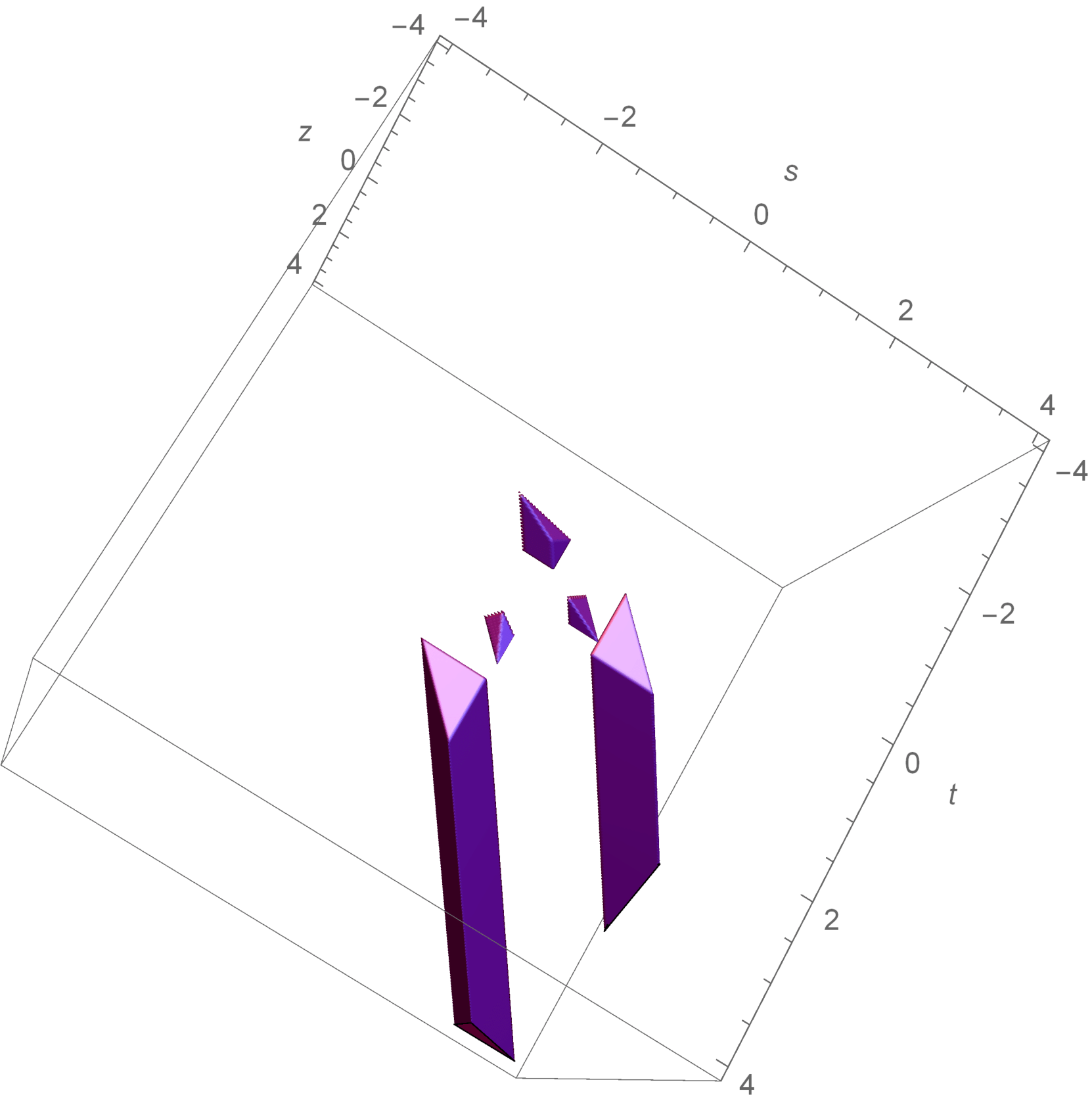
(a) $\check{\mathfrak{K}}$

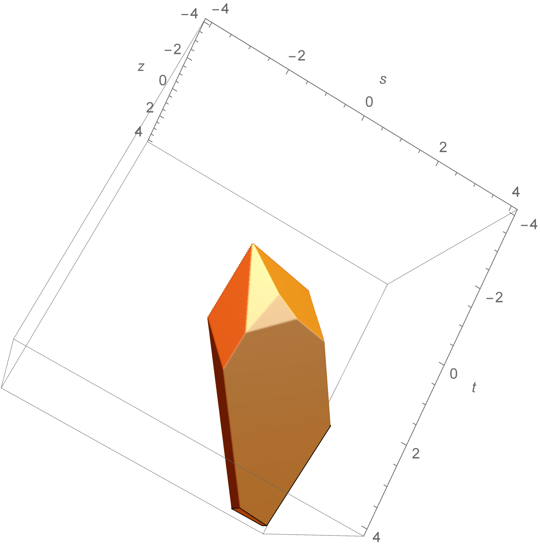
(b) $\check{\mathfrak{K}}_{\text{\rm conv}}$

Figure 3: The sets $\check{\mathfrak{K}}$ and $\check{\mathfrak{K}}_{\text{\rm conv}}$.

Applying the affine transformation (7.2) to this description, we get that $\check{\mathfrak{K}}^{\prime}_{\text{\rm conv}}$ consists of the triples $(\sigma,\tau,\theta)\in{\mathbb{R}}^{3}$ satisfying the following conditions:

$$\tfrac{\sigma-\tau}{2}-1,\tfrac{\tau-\sigma}{2},\tfrac{\sigma+\tau-1}{4},\tfrac{3\sigma+\tau-4}{14},\tfrac{\sigma+\tau-1}{2}<\theta<\tfrac{\sigma+\tau+1}{2},\qquad\tau-1<\sigma<\tau+3.$$ (7.5)

Combining (7.4) and (7.5), it follows that $\check{\mathfrak{K}}_{\text{\rm conv}}\cap\check{\mathfrak{K}}^{\prime}_{\text{\rm conv}}$ is given by (1.7) (Fig. 2), completing the proof of Lemma 7.1.

Remark 7.5.

In Sections 6.2.1–6.2.7, we have only written the cases that provide the most general conditions to define ${\mathfrak{S}}_{515},{\mathfrak{S}}_{522},{\mathfrak{S}}_{252},{\mathfrak{S}}_{155},{\mathfrak{S}}_{212}$. But indeed much more hidden work was needed to produce this shorter proof:

• We have computed all cases in Sections 6.2.1–6.2.7, giving rise to seven long lists of conditions that guarantee (6.18) when $m\geq n$.

• We have studied which of those conditions are the most general ones on every ${\mathbb{R}}^{2}\times Q_{ijk}$, for all $ijk=1,\dots,5$. This produces $125$ sets ${\mathfrak{S}}_{ijk}$, whose inverse images by (7.1) give 125 sets ${\mathfrak{K}}_{ijk}$. The corresponding unions are denoted by ${\mathfrak{S}}$ and ${\mathfrak{K}}$, and their convex hulls by ${\mathfrak{S}}_{\text{\rm conv}}$ and ${\mathfrak{K}}_{\text{\rm conv}}$.

• We got that 41 sets ${\mathfrak{K}}_{ijk}$ are empty, including the 25 sets of the form ${\mathfrak{K}}_{ij1}$, and the remaining 84 sets ${\mathfrak{K}}_{ijk}$ fit together forming a “semi-infinite bar” (Fig. 4).

• With tedious computations, we have shown that ${\mathfrak{K}}_{\text{\rm conv}}$ is given by (7.4).

• We have chosen the most simple family, ${\mathfrak{K}}_{515}$, ${\mathfrak{K}}_{522}$, ${\mathfrak{K}}_{252}$, ${\mathfrak{K}}_{155}$, ${\mathfrak{K}}_{212}$, defining the same convex hull ($\check{\mathfrak{K}}_{\text{\rm conv}}={\mathfrak{K}}_{\text{\rm conv}}$).

• Finally, we have made some attempts to improve the estimates of Section 6.2.7 by using more general versions of the Hölder inequality [7]. Some better estimates were obtained in this way, but they produce the same set ${\mathfrak{K}}_{\text{\rm conv}}$ after taking the convex hull.

Remark 7.6.

The set ${\mathfrak{S}}_{\text{\rm conv}}$ may have a simple expression, like ${\mathfrak{K}}_{\text{\rm conv}}$, but its computation became too involved. This is the reason we have used ${\mathfrak{K}}_{\text{\rm conv}}$, obtaining the conditions of Theorem 1.3, which are general enough for our applications in [4]. But, of course, the inverse image of ${\mathfrak{S}}_{\text{\rm conv}}$ by (7.1) is possibly larger than ${\mathfrak{K}}_{\text{\rm conv}}$. Therefore a simple expression of ${\mathfrak{S}}_{\text{\rm conv}}$ would possibly give a better version of Theorem 1.3. Even a simple expression of $\check{\mathfrak{S}}_{\text{\rm conv}}$ would possibly give a better version of Theorem 1.3.

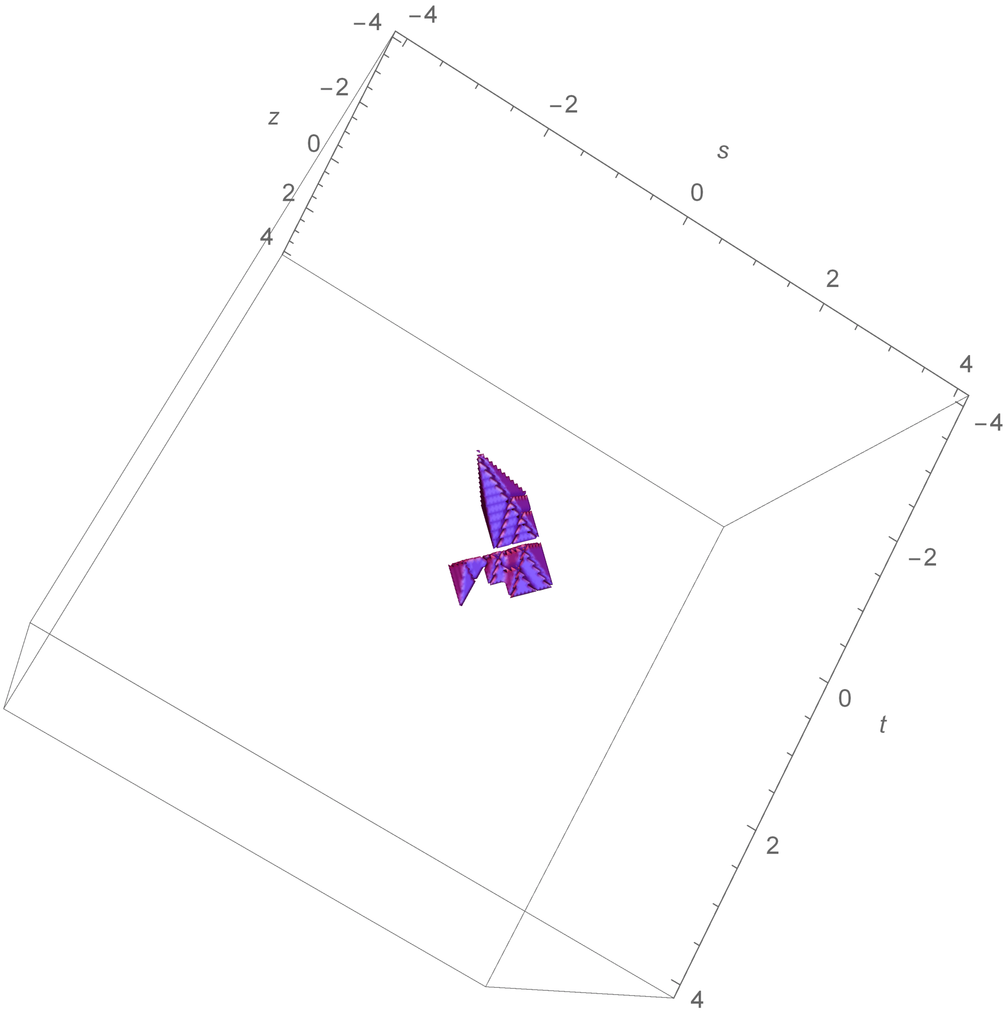
(a) $\bigcup_{i,j}{\mathfrak{K}}_{ij2}$

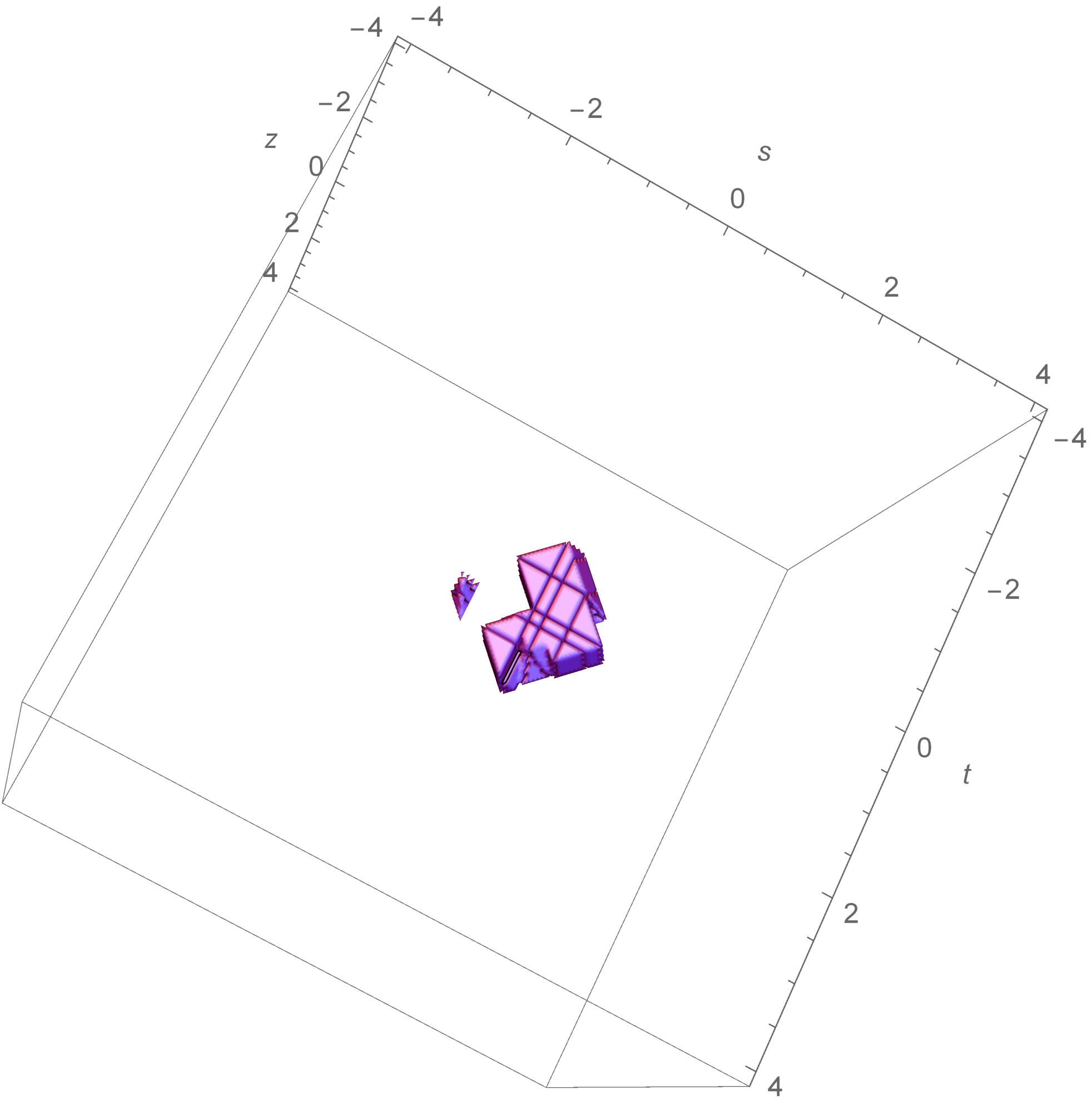
(b) $\bigcup_{i,j}{\mathfrak{K}}_{ij3}$

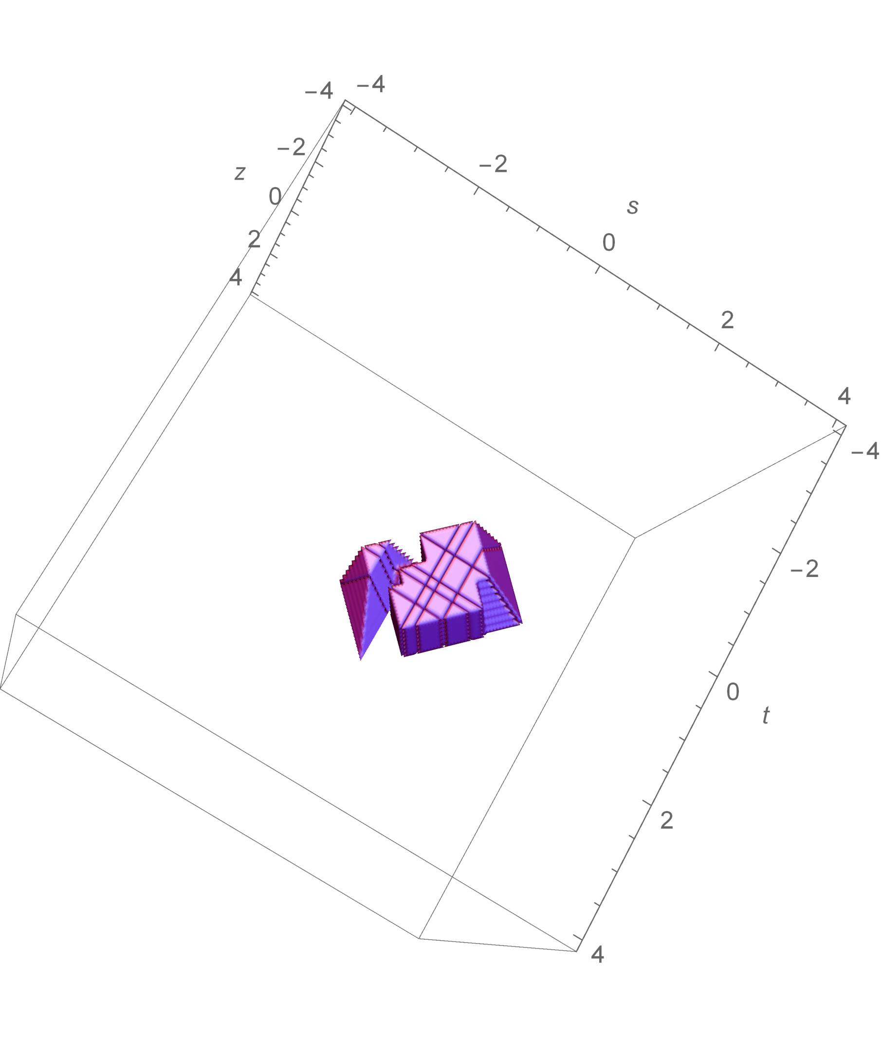
(c) $\bigcup_{i,j}{\mathfrak{K}}_{ij4}$

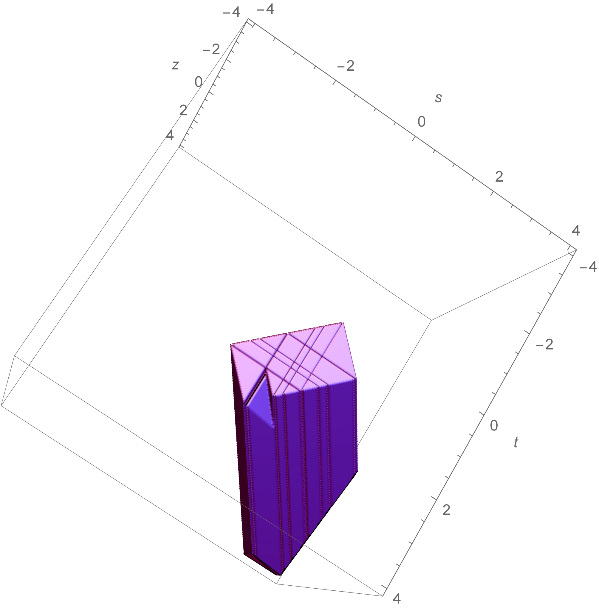
(d) $\bigcup_{i,j}{\mathfrak{K}}_{ij5}$

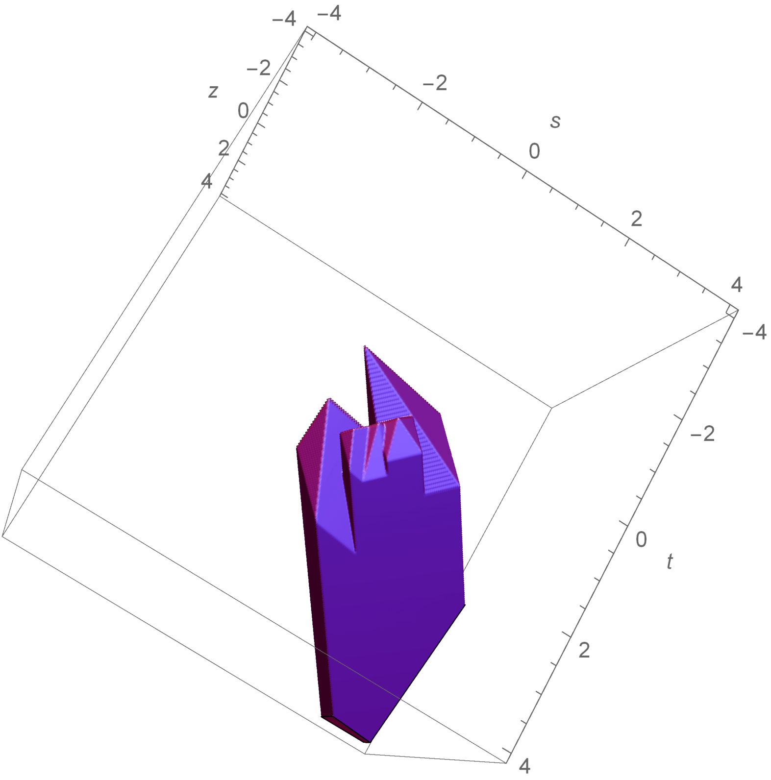
(e) ${\mathfrak{K}}$

Figure 4: Construction of ${\mathfrak{K}}$.

8 Operators induced on $\boldsymbol{{\mathbb{R}}_{+}}$

Let ${\mathcal{S}}_{\text{\rm ev/odd},+}=\{\phi|_{{\mathbb{R}}_{+}}\,|\,\phi\in{\mathcal{S}}_{\text{\rm ev/odd}}\}$. For $c,d>-\frac{1}{2}$, let $L^{2}_{c,+}=L^{2}({\mathbb{R}}_{+},x^{2c}dx)$ and $L^{2}_{c,d,+}=L^{2}_{c,+}\oplus L^{2}_{d,+}$, whose scalar products are denoted by $\langle\ ,\ \rangle_{c}$ and $\langle\ ,\ \rangle_{c,d}$, respectively. For $c_{1},c_{2},d_{1},d_{2}\in{\mathbb{R}}$, let

$$P_{0}=H-2c_{1}x^{-1}\frac{d}{dx}+c_{2}x^{-2},\qquad Q_{0}=H-2d_{1}\frac{d}{dx}x^{-1}+d_{2}x^{-2}.$$

Morever let $\xi>0$ and $\eta,\theta\in{\mathbb{R}}$.

Corollary 8.1.

If $a^{2}+(2c_{1}-1)a-c_{2}=0$, $0<u<1$ and $\sigma:=a+c_{1}>u-\frac{1}{2}$, then there is a positive self-adjoint operator ${\mathcal{P}}$ in $L^{2}_{c_{1},+}$ satisfying the following:

• $x^{a}{\mathcal{S}}_{\text{\rm ev},+}$ is a core of ${{\mathcal{P}}}^{1/2}$ and, for all $\phi,\psi\in x^{a}{\mathcal{S}}_{\text{\rm ev},+}$,

  $$\big{\langle}{{\mathcal{P}}}^{1/2}\phi,{{\mathcal{P}}}^{1/2}\psi\big{\rangle}_{c_{1}}=\langle P_{0}\phi,\psi\rangle_{c_{1}}+\xi\big{\langle}x^{-u}\phi,x^{-u}\psi\big{\rangle}_{c_{1}}.$$

• ${\mathcal{P}}$ has a discrete spectrum. Let $\lambda_{0}\leq\lambda_{2}\leq\cdots$ be its eigenvalues, repeated according to their multiplicity. There is some $D=D(\sigma,u)>0$, and, for each $\epsilon>0$, there is some $C=C(\epsilon,\sigma,u)>0$ so that (1.2) holds for all $k\in 2{\mathbb{N}}$.

Corollary 8.2.

If $b^{2}+(2d_{1}+1)b-d_{2}=0$, $0<u<1$ and $\tau:=b+d_{1}>u-\frac{3}{2}$, then there is a positive self-adjoint operator ${\mathcal{Q}}$ in $L^{2}_{d_{1},+}$ satisfying the following:

• $x^{b}{\mathcal{S}}_{\text{\rm odd},+}$ is a core of ${{\mathcal{Q}}}^{1/2}$ and, for all $\phi,\psi\in x^{b}{\mathcal{S}}_{\text{\rm odd},+}$,

  $$\big{\langle}{{\mathcal{Q}}}^{1/2}\phi,{{\mathcal{Q}}}^{1/2}\psi\big{\rangle}_{d_{1}}=\langle Q_{0}\phi,\psi\rangle_{d_{1}}+\xi\big{\langle}x^{-u}\phi,x^{-u}\psi\big{\rangle}_{d_{1}}.$$

• ${\mathcal{Q}}$ has a discrete spectrum. Let $\lambda_{1}\leq\lambda_{3}\leq\cdots$ be its eigenvalues, repeated according to their multiplicity. There is some $D=D(\tau,u)>0$, and, for each $\epsilon>0$, there is some $C=C(\epsilon,\tau,u)>0$ so that (1.2) holds for all $k\in 2{\mathbb{N}}+1$, with $\tau$ instead of $\sigma$.

Corollary 8.3.

Under the conditions of Corollaries 8.1 and 8.2, if moreover the conditions of Theorem 1.3 are satisfied with some $\theta>-\frac{1}{2}$, then there is a positive self-adjoint operator ${\mathcal{W}}$ in $L^{2}_{c_{1},d_{1},+}$ satisfying the following:

• $x^{a}{\mathcal{S}}_{\text{\rm ev},+}\oplus x^{b}{\mathcal{S}}_{\text{\rm odd},+}$ is a core of ${\mathcal{W}}^{1/2}$, and, for $\phi=(\phi_{1},\phi_{2})$ and $\psi=(\psi_{1},\psi_{2})$ in $x^{a}{\mathcal{S}}_{\text{\rm ev},+}\oplus x^{b}{\mathcal{S}}_{\text{\rm odd},+}$,

  $$\big{\langle}{{\mathcal{W}}}^{1/2}\phi,{{\mathcal{W}}}^{1/2}\psi\big{\rangle}_{c_{1},d_{1}}=\langle(P_{0}\oplus Q_{0})\phi,\psi\rangle_{c_{1},d_{1}}+\xi\big{\langle}x^{-u}\phi,x^{-u}\psi\big{\rangle}_{c_{1},d_{1}}$$

  $$\hphantom{\langle{{\mathcal{W}}}^{1/2}\phi,{{\mathcal{W}}}^{1/2}\psi\rangle_{c_{1},d_{1}}=}{}+\eta\big{(}\big{\langle}x^{-a-b-1}\phi_{2},\psi_{1}\big{\rangle}_{\theta}+\big{\langle}\phi_{1},x^{-a-b-1}\psi_{2}\big{\rangle}_{\theta}\big{)}.$$ (8.1)

• ${\mathcal{W}}$ has a discrete spectrum. Its eigenvalues form two groups, $\lambda_{0}\leq\lambda_{2}\leq\cdots$ and $\lambda_{1}\leq\lambda_{3}\leq\cdots$, repeated according to their multiplicity, such that there is some $D=D(\sigma,\tau,u)>0$ and, for every $\epsilon>0$, there are some $C=C(\epsilon,\sigma,\tau,u)>0$ and $E=E(\epsilon,\sigma,\tau,\theta)>0$ so that (1.9) and (1.10) hold for all $k\in{\mathbb{N}}$.

• If $\tilde{u}\in{\mathbb{R}}$ satisfies (1.11), then there is some $D=D(\sigma,\tau,u)>0$ and, for any $\epsilon>0$, there is some $\widetilde{C}=\widetilde{C}(\epsilon,\sigma,\tau,u)>0$ so that (1.12) holds for all $k\in{\mathbb{N}}$.

• If $u=\frac{v+1}{2}$ and $\xi\geq|\eta|$, then there is some $\widetilde{D}=\widetilde{D}(\sigma,\tau,u)>0$ so that (1.13) holds for all $k\in{\mathbb{N}}$.

• If we add the term $\xi^{\prime}\langle\phi_{1},\psi_{1}\rangle_{c_{1}}+\xi^{\prime\prime}\langle\phi_{2},\psi_{2}\rangle_{d_{1}}$ to the right hand side of (8.1), for some $\xi^{\prime},\xi^{\prime\prime}\in{\mathbb{R}}$, then the result holds as well with the additional term $\max\{\xi^{\prime},\xi^{\prime\prime}\}$ in the right hand side of (1.10), and the additional term, $\xi^{\prime}$ for $k\in 2{\mathbb{N}}$ and $\xi^{\prime\prime}$ for $k\in 2{\mathbb{N}}+1$, in the right hand sides of (1.9), (1.12) and (1.13).

These corollaries follow directly from Theorems 1.1 and 1.3 because the given conditions on $a$ and $b$ characterize the cases where $P_{0}$ and $Q_{0}$ correspond to $|x|^{a}U_{\sigma,\text{\rm ev}}|x|^{-a}$ and $|x|^{b}U_{\tau,\text{\rm odd}}|x|^{-b}$, respectively, via the isomorphisms $|x|^{a}{\mathcal{S}}_{\text{\rm ev}}\to x^{a}{\mathcal{S}}_{\text{\rm ev},+}$ and $|x|^{b}{\mathcal{S}}_{\text{\rm odd}}\to x^{b}{\mathcal{S}}_{\text{\rm odd},+}$ defined by restriction [3, Theorem 1.4 and Section 5]. In fact, Corollaries 8.1 and 8.2 are equivalent because, if $c_{1}=d_{1}+1$ and $c_{2}=d_{2}$, then $Q_{0}=xP_{0}x^{-1}$ and $x\colon L^{2}_{c_{1},+}\to L^{2}_{d_{1},+}$ is a unitary operator.

Remarks 1.2(ii) and 3.21 have obvious versions for these corollaries. In particular, ${\mathcal{P}}=\overline{P}$, ${\mathcal{Q}}=\overline{Q}$ and ${\mathcal{W}}=\overline{W}$, where $P=P_{0}+\xi x^{-2u}$, $Q=Q_{0}+\xi x^{-2u}$ and

$$W=\begin{pmatrix}P&\eta x^{2(\theta-\sigma)+a-b-1}\\ \eta x^{2(\theta-\tau)+b-a-1}&Q\end{pmatrix}=\begin{pmatrix}P&\eta x^{2(\theta-c_{1})-a-b-1}\\ \eta x^{2(\theta-d_{1})-a-b-1}&Q\end{pmatrix},$$

with ${\mathsf{D}}(P)=\bigcap_{m=0}^{\infty}{\mathsf{D}}({{\mathcal{P}}}^{m})$, ${\mathsf{D}}(Q)=\bigcap_{m=0}^{\infty}{\mathsf{D}}({{\mathcal{Q}}}^{m})$ and ${\mathsf{D}}(W)=\bigcap_{m=0}^{\infty}{\mathsf{D}}({{\mathcal{W}}}^{m})$. According to Remark 1.4(ii), we can write (8.1) as

$$\big{\langle}{\mathcal{W}}^{1/2}\phi,{\mathcal{W}}^{1/2}\psi\big{\rangle}_{c_{1},d_{1}}=\langle(P_{0}\oplus Q_{0})\phi,\psi\rangle_{c_{1},d_{1}}+\xi\big{\langle}x^{-u}\phi,x^{-u}\psi\big{\rangle}_{c_{1},d_{1}}$$

$$\hphantom{\big{\langle}{\mathcal{W}}^{1/2}\phi,{\mathcal{W}}^{1/2}\psi\big{\rangle}_{c_{1},d_{1}}=}{}+\eta\big{(}\big{\langle}x^{-a-b+1}\phi_{2},\psi_{1}\big{\rangle}_{\theta^{\prime}}+\big{\langle}\phi_{1},x^{-a-b+1}\psi_{2}\big{\rangle}_{\theta^{\prime}}\big{)},$$

and we have

$$W=\begin{pmatrix}P&\eta x^{2(\theta^{\prime}-c_{1})-a-b+1}\\ \eta x^{2(\theta^{\prime}-d_{1})-a-b+1}&Q\end{pmatrix}.$$

9 Application to the Witten’s perturbation on strata

Let $M$ be a Riemannian $n$-manifold. Let $d$, $\delta$ and $\Delta$ denote the de Rham derivative and coderivative, and the Laplacian, with domain the graded space $\Omega_{0}(M)$ of compactly supported differential forms, and let $L^{2}\Omega(M)$ be the graded Hilbert space of square integrable differential forms. Any closed extension ${\mathbf{d}}$ of $d$ in $L^{2}\Omega(M)$, defining a complex (${\mathbf{d}}^{2}=0$), is called an ideal boundary condition (i.b.c.) of $d$, which defines a self-adjoint extension $\boldsymbol{\Delta}={\mathbf{d}}^{*}{\mathbf{d}}+{\mathbf{d}}{\mathbf{d}}^{*}$ of $\Delta$, called the Laplacian of ${\mathbf{d}}$. There always exists a minimum/maximum i.b.c., $d_{\min}=\overline{d}$ and $d_{\max}=\delta^{*}$, whose Laplacians are denoted by $\Delta_{\min/\max}$. We get corresponding cohomologies $H_{\min/\max}(M)$, and versions of Betti numbers and Euler characteristic, $\beta^{i}_{\min/\max}$ and $\chi_{\min/\max}$. These are quasi-isometric invariants; in particular, $H_{\max}(M)$ is the usual $L^{2}$ cohomology. If $M$ is complete, then there is a unique i.b.c., but these concepts become interesting in the non-complete case. For instance, if $M$ is the interior of a compact manifold with non-empty boundary, then $d_{\min/\max}$ is defined by taking relative/absolute boundary conditions. Given $s>0$ and $f\in C^{\infty}(M)$, the above ideas can be considered as well for the Witten’s perturbations $d_{s}=e^{-sf}de^{sf}=d+sdf\wedge$, with formal adjoint $\delta_{s}=e^{sf}\delta e^{-sf}=\delta-sdf\lrcorner$ and Laplacian $\Delta_{s}$. In fact, this theory can be considered for any elliptic complex.

On the other hand, let us give a rough idea of the concept of stratified space. It is a Hausdorff, locally compact and second countable space $A$ with a partition into $C^{\infty}$ manifolds (strata) satisfying certain conditions. An order on the family of strata is defined so that $X\leq Y$ means that $X\subset\overline{Y}$. With this order relation, the maximum length of chains of strata is called the depth of $A$. Then we continue describing $A$ by induction on $\operatorname{depth}A$, as well as its group $\operatorname{Aut}(A)$ of automorphisms. If $\operatorname{depth}A=0$, then $A$ is just a $C^{\infty}$ manifold, whose automorphisms are its diffeomorphisms. Now, assume that $\operatorname{depth}A>0$, and the descriptions are given for lower depth. Then it is required that each stratum $X$ has an open neighborhood $T$ (a tube) that is a fiber bundle whose typical fiber is a cone $c(L)=(L\times[0,\infty))/(L\times\{0\})$ and structural group $c(\operatorname{Aut}(L))$, where $L$ is a compact stratification of lower depth (the link of $X$), and $c(\operatorname{Aut}(L))$ consists of the homeomorphisms $c(\phi)$ of $c(L)$ induced by the maps $\phi\times\operatorname{id}$ on $L\times[0,\infty)$ ($\phi\in\operatorname{Aut}(L)$). The point $*=L\times\{0\}\in c(L)$ is called the vertex. An automorphism of $A$ is a homeomorphism that restricts to diffeomorphisms between the strata, and whose restrictions to their tubes are fiber bundle homomorphisms. This completes the description because the depth is locally finite by the local compactness.

The local trivializations of the tubes can be considered as “stratification charts”, giving a local description of the form ${\mathbb{R}}^{m}\times c(L)$. Via these charts, a stratum $M$ of $A$ corresponds, either to ${\mathbb{R}}^{m}\times\{*\}\equiv{\mathbb{R}}^{m}$, or to ${\mathbb{R}}^{m}\times N\times{\mathbb{R}}_{+}$ for some stratum $N$ of $L$. The concept of general adapted metric on $M$ is defined by induction on the depth. It is any Riemannian metric in the case of depth zero. For positive depth, a Riemannian metric $g$ on $M$ is called a general adapted metric if, on each local chart as above, $g$ is quasi-isometric, either to the flat Euclidean metric $g_{0}$ if $M$ corresponds to ${\mathbb{R}}^{m}$, or to $g_{0}+x^{2u}\tilde{g}+(dx)^{2}$ if $M$ corresponds to ${\mathbb{R}}^{m}\times N\times{\mathbb{R}}_{+}$, where $\tilde{g}$ is a general adapted metric on $N$, $x$ is the canonical coordinate of ${\mathbb{R}}_{+}$, and $u>0$ depends on $M$ and each stratum $X<M$, whose tube is considered to define the chart. This assignment $X\mapsto u$ is called the type of the metric. We omit the term “general” when we take $u=1$ for all strata.

Assuming that $A$ is compact, it is proved in [4] that, for any general adapted metric $g$ on a stratum $M$ of $A$ with numbers $u\leq 1$, the Laplacian $\Delta_{\min/\max}$ has a discrete spectrum, its eigenvalues satisfy a weak version of the Weyl’s asymptotic formula, and the method of Witten is extended to get Morse inequalities involving the numbers $\beta^{i}_{\min/\max}$ and another numbers $\nu^{i}_{\min/\max}$ defined by the local data around the “critical points” of a version of Morse functions on $M$; here, the “critical points” live in the metric completion of $M$. This is specially important in the case of a stratified pseudo-manifold $A$ with regular stratum $M$, where $H_{\max}(M)$ is the intersection homology with perversity depending on the type of the metric [17, 18]. Again, we proceed by induction on the depth to prove these assertions. In the case of depth zero, these properties hold because we are in the case of closed manifolds. Now, assume that the depth is positive, and these properties hold for lower depth. Via a globalization procedure and a version of the Künneth formula, the computations boil down to the case of the Witten’s perturbation $d_{s}$ for a stratum $M=N\times(0,\infty)$ of a cone $c(L)$ with an adapted metric $g=x^{2u}\tilde{g}+(dx)^{2}$, where we consider the “Morse function” $f=\pm x^{2}/2$.

Let $\tilde{d}_{\min/\max}$, $\tilde{\delta}_{\min/\max}$ and $\widetilde{\Delta}_{\min/\max}$ denote the operators defined as above for $N$ with $\tilde{g}$. Take differential forms $0\neq\gamma\in\ker\widetilde{\Delta}_{\min/\max}$, of degree $r$, and $0\neq\alpha,\beta\in{\mathsf{D}}(\widetilde{\Delta}_{\min/\max})$, of degrees $r$ and $r-1$, with $\tilde{d}_{\min/\max}\beta=\mu\alpha$ and $\tilde{\delta}_{\min/\max}\alpha=\mu\beta$ for some $\mu>0$. Since $\widetilde{\Delta}_{\min/\max}$ is assumed to have a discrete spectrum, $L^{2}\Omega(N)$ has a complete orthonormal system consisting of forms of these types. Correspondingly, there is a “direct sum splitting” of $d_{s}$ into the following two types of subcomplexes:

$$\begin{CD}C^{\infty}_{0}({\mathbb{R}}_{+})\,\gamma @>{d_{s,r}}>{}>C^{\infty}_{0}({\mathbb{R}}_{+})\,\gamma\wedge dx,\end{CD}$$

$$\begin{CD}C^{\infty}_{0}({\mathbb{R}}_{+})\,\beta @>{d_{s,r-1}}>{}>C^{\infty}_{0}({\mathbb{R}}_{+})\,\alpha+C^{\infty}_{0}({\mathbb{R}}_{+})\,\beta\wedge dx@>{d_{s,r}}>{}>C^{\infty}_{0}({\mathbb{R}}_{+})\,\alpha\wedge dx.\end{CD}$$

Forgetting the differential form part, they can be considered as two types of simple elliptic complexes of lengths one and two,

$$\begin{CD}C^{\infty}_{0}({\mathbb{R}}_{+})@>{d_{s,r}}>{}>C^{\infty}_{0}({\mathbb{R}}_{+}),\end{CD}$$

$$\begin{CD}C^{\infty}_{0}({\mathbb{R}}_{+})@>{d_{s,r-1}}>{}>C^{\infty}_{0}({\mathbb{R}}_{+})\oplus C^{\infty}_{0}({\mathbb{R}}_{+})@>{d_{s,r}}>{}>C^{\infty}_{0}({\mathbb{R}}_{+}).\end{CD}$$

Let $\kappa=(n-2r-1)\frac{u}{2}$. In the complex of length one, $d_{s,r}$ is a densely defined operator of $L^{2}_{\kappa,+}$ to $L^{2}_{\kappa,+}$, we have

$$d_{s,r}=\frac{d}{dx}\pm sx,\qquad\delta_{s,r}=-\frac{d}{dx}-2\kappa x^{-1}\pm sx,$$

and the corresponding components of the Laplacian are

$$\Delta_{s,r}=H-2\kappa x^{-1}\frac{d}{dx}\mp s(1+2\kappa),\qquad\Delta_{s,r+1}=H-2\kappa\frac{d}{dx}x^{-1}\mp s(-1+2\kappa).$$

Up to the constant terms, these operators are of the form already considered in [3], without the term with $x^{-2u}$, and the spectrum of $\Delta_{s,\min/\max,r}$ and $\Delta_{s,\min/\max,r+1}$ is well known.

Table 1: Self-adjoint extensions of $\Delta_{s,r-1}$ and $\Delta_{s,r+1}$.

$a$	$\sigma$	condition	$b$	$\tau$	condition
$0$	$\kappa+u$	$\kappa>-\frac{1}{2}$	$0$	$\kappa$	$\kappa>u-\frac{3}{2}$
$1-2(\kappa+u)$	$1-\kappa-u$	$\kappa<\frac{3}{2}-2u$	$1-2\kappa$	$-1-\kappa$	$\kappa<\frac{1}{2}-u$

Table 2: Self-adjoint extensions of $\Delta_{s,r}$.

$a$	$b$	$\sigma$	$\tau$	$\theta$	Condition
$0$	$0$	$\kappa$	$\kappa+u$	$\kappa$	$\kappa>u-\frac{1}{2}$
$1-2\kappa$	$-1-2(\kappa+u)$	$1-\kappa$	$-1-\kappa-u$	$-\kappa-u$	$\kappa<\frac{1}{2}-2u$
$0$	$-1-2(\kappa+u)$	$\kappa$	$-1-\kappa-u$	$-\frac{1}{2}-u$	Impossible
$1-2\kappa$	$0$	$1-\kappa$	$\kappa+u$	$\frac{1}{2}$	$-1-\frac{u}{2}<\kappa<1-\frac{u}{2}$

In the complex of length two, $d_{s,r-1}$ is a densely defined operator of $L^{2}_{\kappa+u,+}$ to $L^{2}_{\kappa,+}\oplus L^{2}_{\kappa+u,+}$, $d_{s,r}$ is a densely defined operator of $L^{2}_{\kappa,+}\oplus L^{2}_{\kappa+u,+}$ to $L^{2}_{\kappa,+}$, we have

$$d_{s,r-1}=\begin{pmatrix}\mu\\ \frac{d}{dx}\pm sx\end{pmatrix},\qquad\delta_{s,r-1}=\begin{pmatrix}\mu x^{-2u}&-\frac{d}{dx}-2(\kappa+u)x^{-1}\pm sx\end{pmatrix},$$

$$d_{s,r}=\begin{pmatrix}\frac{d}{dx}\pm sx&-\mu\end{pmatrix},\qquad\delta_{s,r}=\begin{pmatrix}-\frac{d}{dx}-2\kappa x^{-1}\pm sx\\ -\mu x^{-2u}\end{pmatrix},$$

and the corresponding components of the Laplacian are

$$\Delta_{s,r-1}=H-2(\kappa+u)x^{-1}\frac{d}{dx}+\mu^{2}x^{-2u}\mp s(1+2(\kappa+u)),$$

$$\Delta_{s,r+1}=H-2\kappa\frac{d}{dx}x^{-1}+\mu^{2}x^{-2u}\mp s(-1+2\kappa),$$

$$\Delta_{s,r}=\begin{pmatrix}A&-2\mu ux^{-1}\\ -2\mu ux^{-2u-1}&B\end{pmatrix},$$

where

$$A=H-2\kappa x^{-1}\frac{d}{dx}+\mu^{2}x^{-2u}\mp s(1+2\kappa),$$

$$B=H-2(\kappa+u)\frac{d}{dx}x^{-1}+\mu^{2}x^{-2u}\mp s(-1+2(\kappa+u)).$$

Up to the constant terms, $\Delta_{s,r-1}$ and $A$ are of the form of $P$, and $\Delta_{s,r+1}$ and $B$ are of the form of $Q$, in Section 8. In the case $u=1$, these operators were studied in [3]. Thus assume that $u<1$. Then, according to Corollaries 8.1–8.3, we get self-adjoint extensions of $\Delta_{s,r-1}$, $\Delta_{s,r+1}$ and $\Delta_{s,r}$ as indicated in Tables 1 and 2, where the conditions are determined by the hypotheses; indeed most possibilities of the hypothesis are needed. With further analysis [4], the maximum and minimum Laplacians can be given by appropriate choices of these operators, depending on the values of $\kappa$. Moreover the eigenvalue estimates of these corollaries play a key role in this research.

If $A$ is a stratified pseudo-manifold, our restrictions on $u$ allow to get enough metrics to represent all intersection cohomologies of $A$ with perversity less or equal than the lower middle perversity, according to [17, 18].

Acknowledgements

The first author was partially supported by MICINN, Grants MTM2011-25656 and MTM2014-56950-P, and by Xunta de Galicia, Grant Consolidación e estructuración 2015 GPC GI-1574. The third author has received financial support from the Xunta de Galicia and the European Union (European Social Fund - ESF).

References

[1]
Álvarez López J., Calaza M., Application of the method of Bonan–Clark
to the generalized Hermite polynomials, arXiv:1101.5022.
[2]
Álvarez López J., Calaza M., Witten’s perturbation on strata,
Asian J. Math., to appear, arXiv:1205.0348.
[3]
Álvarez López J., Calaza M., Embedding theorems for the Dunkl harmonic
oscillator, SIGMA10 (2014), 004, 16 pages,
arXiv:1301.4196.
[4]
Álvarez López J., Calaza M., Franco C., Witten’s perturbation on strata with
general adapted metrics, in preparation.
[5]
Askey R., Wainger S., Mean convergence of expansions in Laguerre and Hermite series,
Amer. J. Math.87 (1965), 695–708.
[6]
Brasselet J.P., Hector G., Saralegi M., -cohomologie des espaces stratifiés,
Manuscripta Math.76 (1992), 21–32.
[12]
Erdélyi A., Asymptotic forms for Laguerre polynomials,
J. Indian Math. Soc.24 (1960), 235–250.
[13]
Genest V.X., Vinet L., Zhedanov A., The singular and the anisotropic
Dunkl oscillators in the plane, J. Phys. A: Math. Theor.46 (2013), 325201, 17 pages, arXiv:1305.2126.
[14]
Kato T., Perturbation theory for linear operators, Classics in Mathematics,
Springer-Verlag, Berlin, 1995.
[15]
Muckenhoupt B., Asymptotic forms for Laguerre polynomials,
Proc. Amer. Math. Soc.24 (1970), 288–292.
[16]
Muckenhoupt B., Mean convergence of Laguerre and Hermite series. II,
Trans. Amer. Math. Soc.147 (1970), 433–460.
[17]
Nagase M., -cohomology and intersection homology of stratified spaces,
Duke Math. J.50 (1983), 329–368.
[18]
Nagase M., Sheaf theoretic -cohomology, in Complex Analytic
Singularities, Adv. Stud. Pure Math., Vol. 8, North-Holland,
Amsterdam, 1987, 273–279.
[19]
Nowak A., Stempak K., Imaginary powers of the Dunkl harmonic oscillator,
SIGMA5 (2009), 016, 12 pages, arXiv:0902.1958.
[20]
Nowak A., Stempak K., Riesz transforms for the Dunkl harmonic oscillator,
Math. Z.262 (2009), 539–556, arXiv:0802.0474.
[22]
Reed M., Simon B., Methods of modern mathematical physics. IV. Analysis of
operators, Academic Press, New York – London, 1978.
[23]
Rosenblum M., Generalized Hermite polynomials and the Bose-like oscillator
calculus, in Nonselfadjoint Operators and Related Topics (Beer Sheva,
1992), Oper. Theory Adv. Appl., Vol. 73, Editors A. Feintuch,
I. Gohberg, Birkhäuser, Basel, 1994, 369–396, math.CA/9307224.
[24]
Rösler M., Generalized Hermite polynomials and the heat equation for
Dunkl operators, Comm. Math. Phys.192 (1998), 519–542,
q-alg/9703006.
[25]
Rösler M., Dunkl operators: theory and applications, in Orthogonal
Polynomials and Special Functions (Leuven, 2002), Lecture Notes in
Math., Vol. 1817, Editors E. Koelink, W. Van Assche, Springer, Berlin, 2003,
93–135, math.CA/0210366.
[26]
Szegő G., Orthogonal polynomials, American Mathematical Society
Colloquium Publications, Vol. 23, 4th ed., Amer. Math. Soc., Providence,
R.I., 1975.
[27]
van Diejen J.F., Vinet L. (Editors), Calogero–Moser–Sutherland models,
CRM Series in Mathematical Physics, Springer-Verlag, New York, 2000.
[28]
Yang L.M., A note on the quantum rule of the harmonic oscillator, Phys.
Rev.84 (1951), 788–790.