Pseudogap and the specific heat of high T_c superconductors: a Hubbard model in a n-pole approximation

Abstract

In this work the specific heat of a two-dimensional Hubbard model, suitable to discuss high-$T_{c}$ superconductors (HTSC), is studied taking into account hopping to first ($t$) and second ($t_{2}$) nearest neighbors. Experimental results for the specific heat of HTSC’s, for instance, the YBCO and LSCO, indicate a close relation between the pseudogap and the specific heat. In the present work, we investigate the specific heat by the Green’s function method within a $n$-pole approximation. The specific heat is calculated on the pseudogap and on the superconducting regions. In the present scenario, the pseudogap emerges when the antiferromagnetic (AF) fluctuations become sufficiently strong. The specific heat jump coefficient $\Delta\gamma$ decreases when the total occupation per site ($n_{T}$) reaches a given value. Such behavior of $\Delta\gamma$ indicates the presence of a pseudogap in the regime of high occupation.

1 Introduction

The hole-doped high-$T_{c}$ cuprates are characterized by the presence of strong correlations in the underdoped regime where anomalies as the pseudogap are manifested [1]. The normal state pseudogap observed in high-$T_{c}$’s has been intensively studied hoping to get information to help understand the unconventional superconductivity in such systems. The specific heat is a physical quantity that suffers the effects of the pseudogap. Indeed, experimental results for cuprates show that the specific heat is suppressed in the pseudogap region [2, 3]. This occurs because the pseudogap which develops near the Fermi energy depletes the spectral weight and affects the specific heat which is associated to the density of states on the Fermi energy. The pseudogap occurs in the strong coupling regime [4, 5, 6], therefore, it is important to treat problem by using a theoretical technique that take into account the strong correlations in an adequate way. However, much of the theoretical studies of the pseudogap regime are performed considering BCS-like theories [7, 8, 9] which disregard correlations that might be important for the correct description of the pseudogap regime.

In the present work, a two dimensional Hubbard model with hopping to first and second nearest neighbors is investigated by a $n$-pole approximation [10, 11]. Such approximation preserves correlation functions for instance, the spin-spin correlation function $\langle\vec{S}_{j}\cdot\vec{S}_{i}\rangle$, that play an important role in the strong coupling regime. Furthermore, such $n$-pole approximation allow us to consider superconductivity with $d_{x^{2}-y^{2}}$-wave pairing and also to investigate the pseudogap regime of the two dimensional repulsive Hubbard model.

2 Model and formalism

The Hubbard model considered is described by the Hamiltonian:

$$\hat{H}=\sum_{\langle\langle ij\rangle\rangle\sigma}t_{ij}c_{i\sigma}^{{\dagger}}c_{j\sigma}+\frac{U}{2}\sum_{i\sigma}n_{i,\sigma}n_{i,-\sigma}-\mu\sum_{i\sigma}n_{i\sigma}$$ (1)

where $c_{i\sigma}^{{\dagger}}(c_{i\sigma})$ is the fermionic creation (annihilation) operator at site $i$ with spin $\sigma=\{\uparrow,\downarrow\}$ and $n_{i,\sigma}=c_{i\sigma}^{{\dagger}}c_{i\sigma}$ is the number operator. The quantity $t_{ij}$ represents the hopping between sites $i$ and $j$ and $\langle\langle...\rangle\rangle$ indicates the sum over the first and second-nearest-neighbors of $i$. $U$ is the repulsive Coulomb potential between the $c$ electrons localized at the same site $i$ and $\mu$ the chemical potential. The bare dispersion relation is ${\varepsilon}_{\vec{k}}=2t[\cos(k_{x}a)+\cos(k_{y}a)]+4t_{2}\cos(k_{x}a)\cos(k_{y}a)$ where $t$ is the first-neighbor and $t_{2}$ is the second-neighbor hopping amplitudes.

The Green’s function equation of motion

$$\omega\langle\langle\hat{A};\hat{B}\rangle\rangle=\langle[\hat{A};\hat{B}]_{+}\rangle+\langle\langle[\hat{A},\hat{H}];\hat{B}\rangle\rangle$$ (2)

which relates the Hamiltonian $\hat{H}$ and the one-particle Green’s function $\langle\langle\hat{A};\hat{B}\rangle\rangle$ presents the new Green’s function $\langle\langle[\hat{A},\hat{H}];\hat{B}\rangle\rangle$. The equation of motion of this new Green’s function is $\omega\langle\langle[\hat{A},\hat{H}];\hat{B}\rangle\rangle=\langle[[\hat{A},\hat{H}];\hat{B}]_{+}\rangle+\langle\langle[[\hat{A},\hat{H}],\hat{H}];\hat{B}\rangle\rangle$ which involves a second new Green’s function and implies that it is necessary to solve a infinite set of equations. An interesting way to treat this set of equations is a $n$-pole approximation [10, 11] which assumes that the commutator $[\hat{A},\hat{H}]$ can be rewritten as

$$[\hat{A}_{n},\hat{H}]=\sum_{m}K_{nm}\hat{A}_{m}$$ (3)

in which $\{\hat{A}_{n}\}$ is a set of operators describing the most important excitations of the system [11]. The quantity $\bf{K}$ present in equation 3 is determined from the relation $\bf{K}=\bf{E}\bf{N}^{-1}$ with $N_{nm}=\langle[\hat{A}_{n};\hat{A}^{\dagger}_{m}]_{+}\rangle$ and $E_{nm}=\langle[[\hat{A}_{n};\hat{H}];\hat{A}^{\dagger}_{m}]_{+}\rangle$. In this way, the Green’s function matrix is

$$\bf{G}(\omega)=\bf{N}(\omega\bf{N}-\bf{E})^{-1}\bf{N}.$$ (4)

The Green’s functions above contain the band shift $W_{\vec{k}\sigma}$ which can be written as

$$W_{\vec{k}\sigma} = -\frac{1}{\langle n_{i\sigma}\rangle(1-\langle n_{i\sigma}\rangle)}\left\{\sum_{\langle\langle ij\rangle\rangle}t_{ij}\langle c_{i\sigma}^{{\dagger}}c_{j\sigma}(n_{i-\sigma}-n_{j-\sigma})\rangle\right.$$

$$\left.-\sum_{\langle\langle ij\rangle\rangle}e^{i\vec{k}\cdot(\vec{R}_{j}-\vec{R}_{i})}t_{ij}\left[\langle\vec{S}_{j}\cdot\vec{S}_{i}\rangle+\frac{1}{4}(\langle N_{j}N_{i}\rangle-\langle N_{j}\rangle\langle N_{i}\rangle)-\langle c^{\dagger}_{j\sigma}c^{\dagger}_{j-\sigma}c_{i-\sigma}c_{i\sigma}\rangle\right]\right\}$$

where $N_{j}=n_{j\sigma}+n_{j-\sigma}$ is the total number operator. The correlation functions present in $W_{\vec{k}\sigma}$ can be determined self-consistently as in references [10, 11, 12]. In particular, the spin-spin correlation function $\langle\vec{S}_{j}\cdot\vec{S}_{i}\rangle$ plays an important role in the present work because it is related to antiferromagnetic correlations which are one of the sources of a pseudogap [13, 14].

2.1 Specific heat

The specific heat is obtained from the energy per particle as $C=\frac{\partial E}{\partial T}$. Following the procedure described by Kishore and Joshi [15], the energy per particle for the superconducting state of the Hubbard model introduced in equation (1) is:

$$E_{S}=\frac{1}{2L}\sum_{\vec{k},\sigma}\sum_{i=1}^{4}Z_{i,\vec{k}\sigma}(\varepsilon_{\vec{k}}+\mu+E_{i,\vec{k}\sigma})f(E_{i,\vec{k}\sigma})-\mu n_{T}\,$$ (6)

where $n_{T}=n_{-\sigma}+n_{\sigma}$ is the total occupation, $Z_{i,\vec{k}\sigma}$ are the spectral weights [11] of the Green’s function $G^{(11)}_{\vec{k},\sigma}=\langle\langle c_{\vec{k},\sigma};c_{\vec{k},\sigma}^{\dagger}\rangle\rangle$ and $f(\omega)$ is the Fermi function. In the superconducting state, the renormalized bands are:

$$E_{i,\vec{k}\sigma}=(-1)^{(i+1)}\sqrt{\omega_{j,\vec{k}\sigma}^{2}+\,\frac{(-1)^{(j+1)}|\Delta_{\vec{k}}|^{2}[(\varepsilon_{\vec{k}}+Un_{-\sigma}-\mu)^{2}-\omega_{j,\vec{k}\sigma}^{2}]}{n_{-\sigma}^{2}(1-n_{-\sigma})^{2}(\omega_{2,\vec{k}\sigma}^{2}-\omega_{1,\vec{k}\sigma}^{2})}}\,,$$ (7)

with $j=1$ if $i=1$ or $2$, and $j=2$ if $i=3$ or $4$, $\Delta_{\vec{k}}=2t\Delta_{0}(cos(k_{x}a)-cos(k_{y}a))$ is the gap function where $\Delta_{0}$ is the superconducting order parameter with $d_{x^{2}-y^{2}}$-wave symmetry[11]. In the normal state, the renormalized bands are:

$$\omega_{j,\vec{k}\sigma}=\frac{U+\varepsilon_{\vec{k}}+W_{\vec{k},\sigma}-2\mu}{2}-(-1)^{(j+1)}\frac{X_{\vec{k},\sigma}}{2}$$ (8)

where $X_{\vec{k}}=\sqrt{(U-\varepsilon_{\vec{k}}+W_{\vec{k}\sigma})^{2}+4\langle n_{-\sigma}\rangle U(\varepsilon_{\vec{k}}-W_{\vec{k}\sigma})}$.

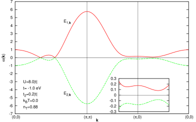
Figure 1: The renormalized bands near the Fermi energy in the superconducting state. The inset shows in detail the gap in the region of the $(\pi,0)$ point.

The specific heat jump is

$$\Delta C=[\frac{(C_{S}-C_{N})}{C_{N}}]_{{}_{T=T_{c}}}$$ (9)

with $C_{S,N}=\frac{\partial E_{S,N}}{\partial T}$ in which $E_{S}$ and $E_{N}$ are the energy per particle in the superconducting and in the normal sate, respectively. $E_{N}$ is obtained from equation (6), but keeping the superconducting order parameter being equal to zero $(\Delta_{0}=0)$.

3 Results

Figure 1 show the bands close to the Fermi energy. Notice that the superconducting gap is present around the point $(\pi,0)$ but it is absent on the $k_{x}=k_{y}$ diagonal. This feature reflects the $d_{x^{2}-y^{2}}$-wave symmetry of the order parameter. The inset shows in detail the neighborhood of the $(\pi,0)$ point.

The normal state renormalized band $\omega_{1,\vec{k}\sigma}$ is shown in figure 2 for different intensities of the total occupation $n_{T}$. It is important to note that although the temperature $k_{B}T=0.04|t|$ is greater than $T_{c}(\lesssim 0.038|t|)$ a gap is still appearing around the point $(\pi,0)$. However, the gap appears only for $n_{T}$ above a given value, in this case $n_{T}\gtrsim 0.81$. A more carefully analysis show that the band crosses to above the chemical potential in the region of the $(\frac{\pi}{2},\frac{\pi}{2})$ point. This feature show that the gap developed in $(\pi,0)$ is actually a pseudogap like those observed in cuprate systems [1]. The inset exhibit in details the pseudogap region (for $n_{T}=0.88$) and shows that the band does not reaches the chemical potential in the range of $\vec{k}$ where the pseudogap occurs.

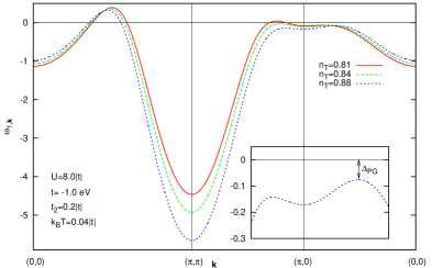
Figure 2: The normal state renormalized band $\omega_{1,\vec{k}\sigma}$ for different intensities of the total occupation $n_{T}$. The inset shows in detail the pseudogap (for $n_{T}=0.88$) that appears in the region around the $(\pi,0)$ point.

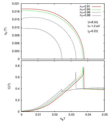
Figure 3: The upper panel shows the order parameter $\Delta_{0}(T)$ as a function of the temperature for several occupations $n_{T}$. The lower panel shows the specific heat for the same parameters as in the upper panel.

The upper panel in figure 3 shows the order parameter $\Delta_{0}$ versus the temperature for different occupations $n_{T}$. The intensity of $\Delta_{0}$ decreases when $n_{T}$ increases leading the system to a regime of strong correlations [4]. The lower panel displays the specific heat $C(T)$ for the same model parameters as in the upper panel. The anomaly on $C(T=T_{c})$ is clearly observed. However, the most important feature in this result, is that, in the range of $n_{T}$ considered in this work, the specific heat jump on $T_{c}$ decreases when $n_{T}$ increases. In order to better understand such behavior, the specific heat jump coefficient $\Delta\gamma=\Delta C(T_{c})/T_{c}$ ( $\Delta C$ is defined in equation (9)) as a function of the total occupation $n_{T}$ is shown in figure 4(a). Notice that initially the $\Delta\gamma$ increases slightly with $n_{T}$ but, above $n_{T}\approx 0.835$, $\Delta\gamma$ starts to decrease. Such behavior for $\Delta\gamma$ is close related to the development of a pseudogap on the density of states (DOS). The pseudogap suppresses the DOS at the chemical potential $\mu$ resulting in a reduction of the $\Delta\gamma$ which should be proportional to the DOS at $\mu$. In figure 4(b) we present the DOS at $\mu$ (DOS_μ) calculated using the same parameters as in 4(a). The decreasing of DOS_μ with $n_{T}$ is directly related to the pseudogap near de chemical potential and agrees with a high-resolution photoemission study [16] of La_2-xSr_xCuO₄ which suggests that a pseudogap is the main responsible for the similar behavior between the specific heat coefficient and the DOS_μ observed in the underdoped regime.

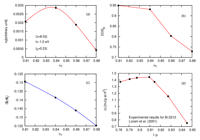
Figure 4: In (a) the specific heat jump coefficient $\Delta\gamma=\Delta C(T_{c})/T_{c}$ as a function of the occupation $n_{T}$. The panels (b) and (c) show respectively the density of states on the chemical potential and the spin-spin correlation function for the same model parameters as in (a). The panel (d) presents experimental results for the jump in the specific heat coefficient $\Delta\gamma$ extracted from figure 3 of reference [3]. p is the hole doping.

Figure 4(c) presents the spin-spin correlation function $\langle\vec{S}_{j}\cdot\vec{S}_{i}\rangle$ for the same model parameters as in 4(a). The $\langle\vec{S}_{j}\cdot\vec{S}_{i}\rangle<0$ is associated to large nearest-neighbor antiferromagnetic correlations. The modulus $|\langle\vec{S}_{j}\cdot\vec{S}_{i}\rangle|$ increases with $n_{T}$ evidencing the presence of strong antiferromagnetic fluctuations in the system. If the antiferromagnetic fluctuations are sufficiently strong it favors the appearance of a pseudogap around the $(\pi,0)$ point (as show in figure 2) and the jump in the specific heat coefficient $\Delta\gamma$ starts to decrease.

The result show for $\Delta\gamma$ presented in 4(a) is in qualitatively agreement with experimental results for cuprates [2, 3]. In panel 4(d) we show the jump in the specific heat coefficient $\Delta\gamma$ extracted from figure 3 of reference [3]. The quantity p indicates the number of holes per CuO₂ atoms.

4 Conclusions

The pseudogap and the superconducting regimes of a two-dimensional Hubbard model that includes hopping to first and second nearest neighbors is investigated. The model has been investigated through a $n$-pole approximation [10, 11] suitable to study the strong correlated regime. The results show that even above $T_{c}$ a gap persists on the region of the $(\pi,0)$ and $(0,\pi)$ points in the first Brillouin zone which is a feature of a pseudogap with $d_{x^{2}-y^{2}}$-wave symmetry. However, the pseudogap develops only above a given occupation $n_{T}$ where the antiferromagnetic fluctuations associated to the spin-spin correlation function $\langle\vec{S}_{j}\cdot\vec{S}_{i}\rangle$ becomes sufficiently strong. Such pseudogap affects the specific heat suppressing the jump in the specific heat coefficient $\Delta\gamma$. The result for $\Delta\gamma$ is in qualitatively agreement with experimental results for some cuprates [2, 3]. In summary, in this work we report some results obtained by treating the Hubbard model within an approximation [10, 11] that is adequate for investigate the strong coupling regime of the model. The obtained results are in qualitatively agreement with some experimental results [2, 3] and are consistent with the recent dynamical cluster approximation (DCA) studies [4, 5, 6] which asserts that the pseudogap at issue is a feature of the strongly coupling regime.

5 Acknowledgment

This work was partially supported by the Brazilian agencies CNPq, CAPES and FAPERGS.

References

- [1] Timusk T and Statt B 1999 Rep. Prog. Phys. 62 61
- [2] Loram J W, Luo J L, Cooper J R, Liang W Y and Tallon J L 2000 Physica C 341 831
- [3] Loram J W, Luo J , Cooper J R, Liang W Y and Tallon J L 2001 J. Phys. Chem. Solids 62 56
- [4] Gull E and Millis A J 2012 Phys. Rev. B 86 241106
- [5] Gull E, Parcollet O and Millis A J 2013 Phys. Rev. Lett. 110 216405
- [6] Gull E and Millis A J 2014 Phys. Rev. B 90 041110
- [7] Tifrea I and Moca C P 2003 Eur. Phys. J. B 35 33
- [8] Pérez L A, Millán J S, Domínguez B C and Wang C 2007 J. Mag. Mag. Mat. 310 129
- [9] Dzhumanov S and Karimboev E X 2014 Physica A 406 176
- [10] Roth L M 1969 Phys. Rev. 184 451
- [11] Beenen J and Edwards D M 1995 Phys. Rev. B 52 13636
- [12] Calegari E J, Magalhaes S G and Gomes A A 2005 Eur. Phys. J. B 45 485
- [13] Kusunose H 2006 J. Phys. Soc. Jpn. 75 054713
- [14] Kyung B, Landry J S and Tremblay A M S 2003 Phys. Rev. B 68 174502
- [15] Kishore R and Joshi S K 1971 J. Phys. C: Solid St. Phys. 4 2475
- [16] Ino A, Mizokawa T, Kobayashi K and Fujimori A 1998 Phys. Rev. Lett. 81 2224