UCLA/14/TEP/108                             SLAC–PUB–16144                                       IPPP/11/82 SB/F/442-14                                      Saclay–IPhT–T14/185 FR-PHENO-2014-002 Extrapolating $W$-Associated Jet-Production Ratios at the LHC

Abstract

Electroweak vector-boson production, accompanied by multiple jets, is an important background to searches for physics beyond the Standard Model. A precise and quantitative understanding of this process is helpful in constraining deviations from known physics. We study four key ratios in $W\,\!+\,n$-jet production at the LHC. We compute the ratio of cross sections for $W\,\!+\,n$- to $W\!+\,(n\!-\!1)$-jet production as a function of the minimum jet transverse momentum. We also study the ratio differentially, as a function of the $W$-boson transverse momentum; as a function of the scalar sum of the jet transverse energy, $H_{\rm T}^{\rm jets}$; and as a function of certain jet transverse momenta. We show how to use such ratios to extrapolate differential cross sections to $W\,\!+\,6$-jet production at next-to-leading order, and we cross-check the method against a direct calculation at leading order. We predict the differential distribution in $H_{\rm T}^{\rm jets}$ for $W\,\!+\,6$ jets at next-to-leading order using such an extrapolation. We use the BlackHat software library together with SHERPA to perform the computations.

I Introduction

Searches for new physics beyond the Standard Model rely on quantitative theoretical predictions for known-physics backgrounds. Such predictions are also important to the emerging precision studies of the Higgs-like boson AtlasHiggs ; CMSHiggs discovered last year, of the top quark, and of the self-interactions of electroweak vector bosons. Signals of new physics typically hide beneath Standard-Model backgrounds in a broad range of search strategies. Sniffing out the signals requires a good quantitative understanding of the backgrounds as well as the corresponding theoretical uncertainties. The challenge of obtaining such an understanding increases with the increasing jet multiplicities used in cutting-edge search strategies. For some search strategies, the uncertainty surrounding predictions of Standard-Model background rates can be lessened by using data-driven estimates; this approach still requires theoretical input to predict the ratios of signal to control processes or regions.

Predictions for Standard-Model rates at the Large Hadron Collider (LHC) require calculations in perturbative QCD, which enters all aspects of short-distance collisions at a hadron collider. Leading-order (LO) predictions in QCD suffer from a strong dependence on the unphysical renormalization and factorization scales. This dependence gets increasingly strong with growing jet multiplicity. Next-to-leading (NLO) calculations reduce this dependence, typically to a 10–15% residual sensitivity, and offer the first quantitatively reliable order in perturbation theory.

Basic measurements of cross sections or differential distributions suffer from a number of experimental and theoretical uncertainties. Ratios of cross sections should be subject to greatly reduced uncertainties, in particular those due to the jet energy scale, lepton efficiency or acceptance, or the proton-proton luminosity. We may also expect ratios to suffer less from theoretical uncertainties due to uncalculated higher-order corrections, though quantifying this reduction is not necessarily easy. In this paper, we study a variety of ratios based on NLO results for $W^{+}\,\!+\,n$-jet and $W^{-}\,\!+\,n$-jet production with $n\leq 5$. We study the so-called jet-production ratio JetProductionRatio : the ratio of $W\,\!+\,n$-jet production to $W\!+\,(n\!-\!1)$-jet production. (This ratio is also sometimes called the “Berends”, “Berends–Giele” or “staircase” ratio.) We study the jet-production ratio for inclusive total cross sections as a function of the minimum jet transverse momentum $p_{\rm T}^{\text{min}}$, and find a remarkable universality for $n>2$. We also study several differential cross sections: with respect to the vector-boson transverse momentum; with respect to certain jet transverse momenta; and with respect to the total jet transverse energy $H_{\rm T}^{\rm jets}$. Such ratios are also central to data-driven estimates of backgrounds, in which a measurement of one process is used to estimate another. The jet-production ratio is useful for making estimates of backgrounds with additional jets. As an example, we predict the differential distribution in the total jet transverse energy in $W\,\!+\,6$-jet production to NLO accuracy. Englert et al. Englert and Gerwick et al. Gerwick have studied jet-production ratios in vector-boson production and pure-jet production. They found that in QCD one expects a constant ratio for jet production at fixed $p_{\rm T}^{\text{min}}$, when all jets are subject to the same cut. Our results are in agreement with these expectations for a broad range of $p_{\rm T}^{\text{min}}$ values.

There have been many experimental measurements of vector production in association with jets at both the Tevatron and the LHC. Here we focus specifically on measurements of various ratios at the LHC. The CMS collaboration has measured ExptJetProductionRatioLHC the jet-production ratios at the LHC for production in association with a $W$ boson, as well as the ratio of $W\,+\,$jets to $Z\,+\,$jets and the $W$ charge asymmetry as a function of the number of jets. (The usefulness of the charge asymmetry, or $W^{+}/W^{-}$ ratio, in reducing uncertainties was emphasized by Kom and Stirling KomStirling ; it has been computed to NLO for up to five associated jets W4j ; W5j .) More recently, CMS measured the $Z/\gamma$ ratio as a function of jets CMSZgamma ; this ratio has also played a role in CMS’s determination of the $Z(\to\nu\nu)\,+\,$jets background to supersymmetry searches CMSSUSY (see also ref. AskEtal ). The ATLAS collaboration has recently presented studies of vector-boson production in association with jets ATLASRatios , as well as measuring the ratio $W/Z$ in association with up to four jets and comparing it with NLO predictions Aad2014rta .

NLO QCD predictions for production of vector bosons with a lower multiplicity of jets (one or two jets) have been available for many years MCFM ; FernandoWjetpapers . In recent years, the advent of new on-shell techniques (see refs. RecentOnShellReviews for recent reviews) for computing one-loop amplitudes at larger multiplicity has also made possible NLO results for three W3jPRL ; W3jDistributions ; EMZW3j ; BlackHatZ3jet , four W4j ; Z4j and even five associated jets W5j . High-multiplicity NLO results have been used to study the jet-production ratios for $W$-boson production in association with up to four jets W3jDistributions ; W4j , but at a single value of $p_{\rm T}^{\text{min}}$.

Here we use on-shell techniques and employ the same computational setup as in ref. W5j . An NLO QCD result is comprised of virtual, Born, and real-emission contributions, along with appropriate infrared subtraction terms. We compute the virtual corrections numerically using the BlackHat code BlackHatI . For processes with up to three associated jets, we use the AMEGIC++ package Amegic to compute Born and real-emission contributions along with their Catani–Seymour CS infrared subtraction terms. For four or five associated jets, we use the COMIX package Comix . We use SHERPA Sherpa to manage the overall calculation, including the integration over phase space AntennaIntegrator . To facilitate new studies with different (tighter) cuts, different scale choices or PDF sets, we store intermediate results: we record the momenta for all partons along with matrix-element information, including the coefficients of various scale- or PDF-dependent functions, in root-format ROOT files NtuplesNote . This makes it possible to evaluate cross sections and distributions for different scales and PDF error sets without re-running from scratch. Experiments have made use of this ability in applying BlackHat predictions. (See, for example, ref. NTupleUse .)

In carrying out the computations for this study, we neglect a number of small contributions. For four and five associated jets, we make use of a leading-color approximation for the virtual contributions that has been validated for processes with up to four jets, with corrections that are under 3% W3jDistributions ; ItaOzeren . We also neglected small contributions from virtual top quarks. In the five-jet case, all four-quark pair terms in the real-emission contributions were also neglected.

This paper is organized as follows. In section II we summarize the basic setup used in the computation. In section III we present our results for cross sections, ratios and distributions. We give our summary and conclusions in section IV. Tables with numerical results are shown in Appendices A–D.

II Basic Setup

In this paper we study ratios involving the $W\,\!+\,n$-jet processes with $n\leq 5$ to NLO in QCD. We include the decay of the vector boson ($W^{\pm}$) into a charged lepton and neutrino at the amplitude level, with no on-shell approximations made for the $W$ boson.

We use several standard kinematic variables to characterize scattering events; for completeness we give their definitions here. The pseudorapidity $\eta$ is given by $\eta=-\ln(\tan{\theta}/{2})$, where $\theta$ is the polar angle with respect to the beam axis. We denote the angular separation of two objects (partons, jets or leptons) by $\Delta R=\sqrt{(\Delta\phi)^{2}+(\Delta y)^{2}}$ with $\Delta\phi$ the difference in the azimuthal angles, and $\Delta y$ the difference in the rapidities.

For use in scale choices, we define the quantity

$${\hat{H}}_{\rm T}^{\prime}\equiv\sum_{j}p_{\rm T}^{j}+E_{\rm T}^{W}\,,$$ (1)

where the sum runs over all final-state partons $j$ and $E_{\rm T}^{W}\equiv\sqrt{M_{W}^{2}+(p_{\rm T}^{W})^{2}}$. This transverse energy is a modified version of the simple sum of transverse energies of all massless outgoing partons and leptons. (The particular choice (1) does not bias the leptonic angular distributions in the $W$ rest frame Wpolarization .) For observable distributions, we use the jet-based quantity

$$H_{\rm T}^{\rm jets}\equiv\sum_{j\in{\rm jets}}E_{\rm T}^{j}\,,$$ (2)

the total transverse energy of jets passing all cuts. This quantity, unlike ${\hat{H}}_{\rm T}^{\prime}$, excludes the transverse energy of the vector boson.

In our study, we consider the inclusive processes $pp\rightarrow$ $W\,\!+\,n$ jets at an LHC center-of-mass energy of $\sqrt{s}=7$ TeV for $n\leq 5$, with the following basic set of cuts:

$$\begin{array}[]{lll}E_{\rm T}^{e}>20\hbox{ GeV}\,,\hskip 42.67912pt&|\eta_{e}|<2.5\,,\hskip 42.67912pt&E_{\rm T}^{\nu}>20\hbox{ GeV}\,,\hskip 42.67912pt\\ p_{\rm T}^{\rm jet}>25\hbox{ GeV}\,,\hskip 42.67912pt&|\eta_{\rm jet}|<3\,,\hskip 42.67912pt&M_{\rm T}^{W}>20\hbox{ GeV}\,.\end{array}$$

We define jets using the anti-$k_{\rm T}$ algorithm antikT with parameter $R=0.5$. The jets are ordered in $p_{\rm T}$, and are labeled $i,j=1,2,3,\ldots$ in order of decreasing transverse momentum $p_{\rm T}$, with $1$ being the leading (hardest) jet. The transverse mass of the $W$-boson is computed from the kinematics of its decay products, $W\rightarrow e\nu_{e}$,

$$M_{\rm T}^{W}=\sqrt{2E_{\rm T}^{e}E_{\rm T}^{\nu}(1-\cos(\Delta\phi_{e\nu}))}\,.$$ (3)

At LO, the missing transverse energy, ${{\raise 0.91666pt\hbox to7.95831pt{\hss/\hss}\hbox to0.0pt{\hss$E$}}}_{\rm T}$, is just the neutrino transverse energy, $E_{\rm T}^{\nu}$. Beyond LO, there are small difference, because of the effect of hadronic energy falling outside of the detector. We leave the assessment of this difference to the experimenters. Accordingly, we perform our calculation for a detector with complete coverage for hadrons, so that again ${{\raise 0.91666pt\hbox to7.95831pt{\hss/\hss}\hbox to0.0pt{\hss$E$}}}_{\rm T}$ is the same as $E_{\rm T}^{\nu}$ even at NLO.

As described in ref. NtuplesNote , we save intermediate results in publicly available root-format ROOT $n$-tuple files NtuplesNote in order to facilitate new studies with different (tighter) cuts, different scale choices or PDF sets. These files contain momenta for all partons, along with the coefficients of various scale- or PDF-dependent functions associated with the squared matrix elements. Using these files we can generate cross sections and distributions for different scales and PDF error sets without re-running from scratch. We impose a looser set of cuts when generating the underlying $n$-tuples, restricting only the minimum jet transverse momentum, to $p_{\rm T}^{\rm jet}>25$ GeV. The $n$-tuples also contain the needed information for anti-$k_{T}$, $k_{T}$ and SISCone algorithms JetAlgorithms for $R=0.4,0.5,0.6,0.7$, as implemented in the FASTJET package FastJet . In the SISCone case the merging parameter $f$ is chosen to be $0.75$. This allows the $n$-tuples to be used for studying the effects of varying the jet algorithm. The cuts (II) are imposed only in analyzing the $n$-tuples.

We use the MSTW2008 LO and NLO parton distribution functions (PDFs) MSTW2008 at the respective orders. We use a five-flavor running $\alpha_{s}(\mu)$ and the value of $\alpha_{s}(M_{Z})$ supplied with the parton distribution functions. The lepton-pair invariant mass follows a relativistic Breit-Wigner distribution with width given by $\Gamma_{W}=2.06$ GeV and mass $M_{W}=80.419$ GeV. We take the leptonic decay products to be massless. In this approximation the results for muon final states are of course identical to those for the electron. The other electroweak parameters are also chosen as in ref. W3jDistributions .

As our calculation is a parton-level one, we do not apply corrections due to non-perturbative effects such as those induced by the underlying event or hadronization. For comparisons to experiment it is of course important to account for these, although for the cross-section ratios studied in this paper we do not expect substantial effects.

The light quarks ($u,d,c,s,b$) are all treated as massless. As mentioned in the introduction, we do not include contributions to the amplitudes from a real or virtual top quark; its omission should have a percent-level effect on the cross sections W4j ; Z4j , and presumably even less in ratios. We use a leading-color approximation for the $W\,\!+\,4$- and $W\,\!+\,5$-jet calculations. We also approximate the Cabibbo-Kobayashi-Maskawa matrix by the unit matrix. For the cuts we impose, this approximation results in a change of under 1% in total cross sections for $W\,\!+\,3$-jet production, and should likewise be completely negligible in our study. We also neglected the tiny processes involving eight quarks or anti-quarks in real-emission contributions to $W+5$ jet production.

There have been recent advances in matching parton showers to NNLO predictions and in merging NLO results for different jet multiplicities with parton showers. While matching is suitable for describing the production of a particular final state (say $W\,+\,1$ jet production) at particle level, merging allows the prediction of signatures involving different numbers of final-state jets (like $W\,+\,1$ jet, $W\,+\,2$ jet, etc.) from the same sample of events and with the same formal accuracy. In our study this method will be used to obtain an alternative prediction.

Matching was pioneered by the MC@NLO and POWHEG methods MCNLO ; POWHEG . The multi-scale improved NLO method (MINLO) MINLO , which augments matched NLO calculations with a natural scale choice and Sudakov form factors later evolved into a full matching technique at NNLO NNLOPS . An independent procedure was introduced in ref. UNLOPS .

The first merging methods at LO accuracy were devised a decade ago MLM ; CKKW ; CKKWL . Using MC@NLO and POWHEG matching they were recently extended to NLO accuracy MEPSNLO ; UNLOPS ; FXFX , with a substantial gain in theoretical precision. For the predictions included here we use the method presented in ref. MEPSNLO . We utilize NLO matrix elements up to $W\,+\,2$ jets and LO matrix elements up to $W\,+\,4$ jets.

We use the same computational setup as in ref. W5j . The virtual contributions are provided by the BlackHat package which is based on on-shell methods. The BlackHat library has previously been used to generate the virtual contributions to NLO predictions for a variety of processes, including those of pure jets, or jets in association with a vector boson, a photon or a pair of photons W3jDistributions ; BlackHatZ3jet ; W4j ; Z4j ; PhotonZ ; FourJets ; W5j . This library uses on-shell methods which are based on the underlying properties of factorization and unitarity obeyed by any amplitude. (See refs. Primitive ; Zqqgg ; ItaOzeren ; W5j for references to the underlying methods.)

Jets	$W^{-}$ LO	$W^{-}$ NLO	$W^{+}$ LO	$W^{+}$ NLO
1	$284.0(0.1)^{+26.2}_{-24.6}$	$351.2(0.9)^{+16.8}_{-14.0}$	$416.8(0.6)^{+38.0}_{-35.5}$	$516(3)^{+29.}_{-23}$
2	$83.76(0.09)^{+25.45}_{-18.20}$	$83.5(0.3)^{+1.6}_{-5.2}$	$130.0(0.1)^{+39.3}_{-28.1}$	$125.1(0.8)^{+1.8}_{-7.4}$
3	$21.03(0.03)^{+10.66}_{-6.55}$	$18.3(0.1)^{+0.3}_{-1.8}$	$34.72(0.05)^{+17.44}_{-10.75}$	$29.5(0.2)^{+0.4}_{-2.8}$
4	$4.93(0.02)^{+3.49}_{-1.90}$	$3.87(0.06)^{+0.14}_{-0.62}$	$8.65(0.01)^{+6.06}_{-3.31}$	$6.63(0.07)^{+0.21}_{-1.03}$
5	$1.076(0.003)^{+0.985}_{-0.480}$	$0.77(0.02)^{+0.07}_{-0.19}$	$2.005(0.006)^{+1.815}_{-0.888}$	$1.45(0.04)^{+0.12}_{-0.34}$

Table 1: Total cross sections in picobarns, as reported in ref. W5j , for $W\,\!+\,n$ jet production at the LHC at $\sqrt{s}=7$ TeV, using the anti-$k_{T}$ jet algorithm with $R=0.5$, the cuts (II), and the central scale choice $\mu_{R}=\mu_{F}={\hat{H}}_{\rm T}^{\prime}/2$. The NLO results for $W\,\!+\,4,5$-jet production use the leading-color approximation discussed in the text. The numerical integration uncertainty is given in parentheses, and the scale dependence is quoted in superscripts and subscripts.

III Results

The present study, which will illustrate the principles of extrapolating to higher multiplicities, is based on our NLO results for $W\,\!+\,n$-jet production at the LHC with $\sqrt{s}=7$ TeV, as reported in ref. W5j . The results reported there, reproduced in table 1, are for the total cross sections for $W\,\!+\,n$-jet production with the standard minimum jet transverse momentum, $p_{\rm T}^{\rm jet}=25$ GeV. The central value of the renormalization scale $\mu_{R}$ and factorization scale $\mu_{F}$ has been set to ${\hat{H}}_{\rm T}^{\prime}/2$, and the upper and lower uncertainties come from varying $\mu_{R}=\mu_{F}$ by a factor of two in either direction around the central value. The same ratios could be studied in the future at 8, 13, or 14 TeV.

Ratios of cross sections and of distributions are expected to provide a cleaner comparison between experiment and theory than the underlying absolute cross sections from which they are formed. Experimentally, ratios should have reduced dependence on various systematic uncertainties, most notably uncertainty in the jet-energy scale. The theoretical predictions of typical ratios are either independent of $\alpha_{s}$ at leading order, or else behave as ${\cal O}(\alpha_{s})$; accordingly, they usually have a much smaller dependence on the renormalization and factorization scales than the underlying quantities. Ratios also reduce some of the limitations of fixed-order results compared to parton-shower simulations, as well uncertainties from parton-distribution functions KomStirling . We will display two explicit examples of reduced uncertainty with respect to the parton-distribution functions in this section.

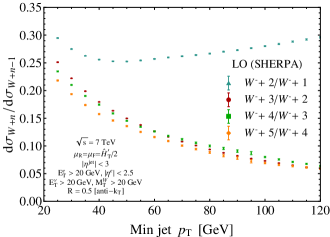
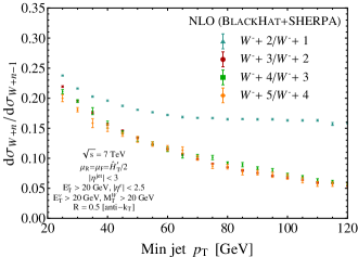
Figure 1: The ratio of the $W^{-}+n$-jet to the $W^{-}+(n-1)$-jet cross section as a function of the minimum jet transverse momentum, $p_{\rm T}^{\text{min}}$. The left plot shows the ratio at LO, and the right plot at NLO. The error bars represent numerical integration errors.

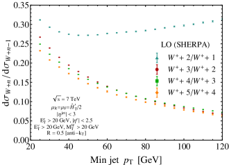
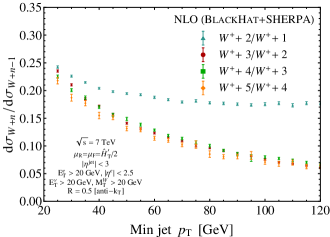
Figure 2: The ratio of the $W^{+}+n$-jet to the $W^{+}+(n-1)$-jet cross section as a function of the minumum jet $p_{\rm T}$. The left plot shows the ratio at LO, and the right plot at NLO.

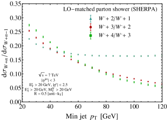
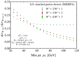
Figure 3: The ratio of the $W+n$-jet to the $W+(n-1)$-jet cross section as a function of the minimum jet transverse momentum, $p_{\rm T}^{\text{min}}$, for a parton shower matched to LO. The left plot shows the ratio for $W^{-}$, and the right plot for $W^{+}$.

III.1 Dependence on Minimum Jet Transverse Momentum

We first examine the dependence of the jet-production ratio on the minimum jet $p_{\rm T}$. We have studied the ratio of $W\,\!+\,n$-jet to $W\!+\,(n\!-\!1)$-jet production at both LO and NLO for a range of minimum jet $p_{\rm T}$s from 25 to 120 GeV. We provide tables of our detailed results in appendix A. We show these data graphically in figs. 1 and 2 as a function of the same cut. We see that the $W\,\!+\,2$-jet to $W\,\!+\,1$-jet ratio is very different from the other ratios. It suffers from large NLO corrections, is numerically quite different, and is flat with increasing jet $p_{\rm T}^{\text{min}}$ (at NLO). In contrast, the ratios of total cross sections for $W\,\!+\,n$-jet to $W\!+\,(n\!-\!1)$-jet production with $n\geq 3$ are similar numerically, fall in a similar manner, and have only modest NLO corrections. Only at the lowest jet $p_{\rm T}^{\text{min}}$ values does the $W\,\!+\,2$-jet to $W\,\!+\,1$-jet ratio take on a value comparable to the other ratios, a similarity which is likely accidental.

The dissimilarity of the $W\,\!+\,2$-jet to $W\,\!+\,1$-jet ratio and the large NLO corrections to it are not surprising. At LO, $W\,\!+\,1$-jet production does not include contributions from the $gg$ initial-state; these arise only at NLO. In contrast, at LO $W\,\!+\,n$-jet production with $n\geq 2$ already includes contributions from all initial-state partons. Furthermore, both $W\,\!+\,1$-jet and $W\,\!+\,2$-jet production suffer from kinematic constraints which are relaxed at NLO. For example, at LO the leading jet in $W\,\!+\,2$-jet production must be opposite in azimuthal angle to the vector boson; at NLO, configurations with the leading jet near the vector boson are possible.

Ratios for $n\geq 3$ are largely independent of $n$ for the range of $p_{\rm T}^{\text{min}}$ values that we have studied. The slight differences between different ratios at LO narrow considerably at NLO. The similarity of ratios suggests a certain universality. The narrowing of differences when going from an LO to an NLO prediction suggests that some of the residual differences at LO are a result of using different renormalization and factorization scales in the numerator and denominator of the ratios, together with the strong scale dependence of the LO cross sections. The similarity is in agreement with the results of refs. Englert ; Gerwick arguing for constant ratios when all jets are subject to an identical $p_{\rm T}^{\text{min}}$ cut, as is the case here.

For comparison, in fig. 3 we show the same ratios computed using the SHERPA parton shower matched to LO. The $W\,\!+\,2$-jet to $W\,\!+\,1$-jet ratio is similar in its $p_{\rm T}^{\text{min}}$ dependence to the NLO result, suggesting that it should not suffer large corrections beyond NLO. The $W\,\!+\,3$-jet to $W\,\!+\,2$-jet and $W\,\!+\,4$-jet to $W\,\!+\,3$-jet ratios are similar in shape to the NLO results, although they are about 20% higher at smaller values of $p_{\rm T}^{\text{min}}$. The LO-matched results are broadly consistent with universality for $n\geq 3$ seen in the NLO prediction. We do not provide ratios for $W\,\!+\,5$-jet production, because of computational limitations with current technology (more specifically, the parton-shower based clustering).

In ref. ExptJetProductionRatioLHC , the dependence of the jet-production ratio on $n$ was studied. This ratio (or rather its inverse) was parametrized as

$$\sigma(\text{$W\,\!+\,n$\ jets})/\sigma(\text{$W\,\!+\,(n\!+\!1)$\ jets})=\alpha+\beta n\,.$$ (4)

The universality of jet-production ratios at different values of $p_{\rm T}^{\text{min}}$ suggests that we try a parametrization that allows us to study their $p_{\rm T}$-dependence. We consider the following parametrization,

$$\sigma(\text{$W\,\!+\,n$\ jets})/\sigma(\text{$W\!+\,(n\!-\!1)$\ jets})=r_{n}(p_{\rm T}^{\text{min}})\,,$$ (5)

where we take the following form for $r_{n}(p)$,

$$r_{n}(p)=b_{n}p^{-\eta_{n}}e^{-d_{n}p}\,.$$ (6)

As explained above, we consider only values of $n$ greater than 1; the $n=1$ case should be treated separately. Our main interest is in the overall power behavior described by the second factor on the right-hand side. We fit $b_{n}$, $\eta_{n}$ and $d_{n}$ to the results for the $W\,\!+\,3$-jet to $W\,\!+\,2$-jet, $W\,\!+\,4$-jet to $W\,\!+\,3$-jet, and $W\,\!+\,5$-jet to $W\,\!+\,4$-jet production ratios (corresponding to the last three columns of the tables in appendix A). A power of $\alpha_{s}$ is absorbed into parameter $b_{n}$.

The form (6) is purely a fit. While it captures the overall features of the curves, it should not be expected to reflect the exact underlying physics. As we increase the statistical precision of the results, the quality of the fit should be expected to decrease. Nonetheless, we can distinguish between fits that do not work at all and those that are reasonable. For example, omitting the last factor in eq. (6) gives very poor fits, with $\chi^{2}$/dof of order $150$ for the $W^{-}\,\!+\,3$-jet to $W^{-}\,\!+\,2$-jet production ratio, for example, whereas the fits of the form in eq. (6) to the LO results give $\chi^{2}$/dof around $2.2$ (or equivalently a likelihood of $3\cdot 10^{-3}$; that is, the probability that the $\chi^{2}$ will exceed $2.2$). While this fit is thus marginal, it is not terrible. The fits to the LO $W^{-}\,\!+\,4$-jet to $W^{-}\,\!+\,3$-jet and $W^{-}\,\!+\,5$-jet to $W^{-}\,\!+\,4$-jet ratios are better. The fits to the NLO results are also better, simply because the statistical uncertainties are larger. (The fits to $W^{+}\,\!+\,n$-jet ratios are all acceptable.) It is remarkable that we obtain such good fits with only three parameters and a simple functional form. Given expected experimental uncertainties, the form in eq. (6) should give a very good fit to experimental data as well.

We perform a logarithmic fit to the form in eq. (6). That is, we perform a linear (least-squares) fit of the log of ratios of $W\,\!+\,n$-jet production to the log of the right-hand side of eq. (6). The results of our fits are shown in table 2 for $W^{-}\,\!+\,n$-jet production, and in table 3 for $W^{+}\,\!+\,n$-jet production. We compute the error estimates using an ensemble of 10,000 fits to synthetic data. Each synthetic data point is taken from a Gaussian distribution with central value given by the computed $W\,\!+\,n$-jet cross section (at the appropriate $p_{\rm T}^{\text{min}}$) and width given by the computed statistical uncertainty in the values underlying the ratios in tables A–A. The cross sections shown in tables A–A for different values of $p_{\rm T}^{\text{min}}$ are not independent, because the same underlying samples of events are used to compute them. Thus, for example, all events that contribute to the cross section with $p_{\rm T}^{\text{min}}=80$ GeV also contribute to the cross section with $p_{\rm T}^{\text{min}}=50$ GeV. For the LO fits, we nonetheless treat the statistical uncertainties as independent, as including the correlations yields only insignificant differences. For the NLO fits, we include the full correlation matrix in generating the synthetic data; this makes a noticeable difference for the $W\,\!+\,4$-jet to $W\,\!+\,3$-jet and $W\,\!+\,5$-jet to $W\,\!+\,4$-jet ratios. (In performing each of the 10,000 fits, the different data points are weighted, in a least-squares procedure, by the diagonal statistical uncertainties, which we treat as independent; this makes only a small difference to the final parameters.) The quoted uncertainties are for each parameter taken independently, and do not take into account any correlations between fit parameters. Two of the fit parameters, $\eta_{n}$ and $b_{n}$, are dimensionless, while $d_{n}$ has units of GeV^-1.

Ratio		Fit Values
		$\eta_{n}$	$d_{n}$	$b_{n}$
$\displaystyle\quad\frac{W^{-}+3}{W^{-}+2}\quad$	LO	$0.480\pm 0.008$	$0.0077\pm 0.0002$	$1.43\pm 0.03$
	NLO	$0.46\pm 0.03$	$0.0074\pm 0.0005$	$1.15{}^{+0.10}_{-0.09}$
$\displaystyle\frac{W^{-}+4}{W^{-}+3}$	LO	$0.48\pm 0.02$	$0.0057\pm 0.0003$	$1.26\pm 0.06$
	NLO	$0.44\pm 0.07$	$0.006\pm 0.001$	$1.0\pm 0.2$
$\displaystyle\frac{W^{-}+5}{W^{-}+4}$	LO	$0.47\pm 0.02$	$0.0064\pm 0.0004$	$1.15{}^{+0.08}_{-0.07}$
	NLO	$0.26\pm 0.12$	$0.009\pm 0.002$	$0.6\pm 0.2$

Table 2: Fit parameters for the jet-production ratio in $W^{-}\,\!+\,n$ jets as a function of the minimum jet $p_{\rm T}$, using the form in eq. (6).

Ratio		Fit Values
		$\eta_{n}$	$d_{n}$	$b_{n}$
$\displaystyle\quad\frac{W^{+}+3}{W^{+}+2}\quad$	LO	$0.457\pm 0.006$	$0.0071\pm 0.0001$	$1.39\pm 0.03$
	NLO	$0.49\pm 0.04$	$0.0060\pm 0.0007$	$1.3{}^{+0.2}_{-0.1}$
$\displaystyle\frac{W^{+}+4}{W^{+}+3}$	LO	$0.459\pm 0.007$	$0.0055\pm 0.0001$	$1.25\pm 0.03$
	NLO	$0.38\pm 0.06$	$0.007\pm 0.001$	$0.9{}^{+0.2}_{-0.1}$
$\displaystyle\frac{W^{+}+5}{W^{+}+4}$	LO	$0.42\pm 0.02$	$0.0066\pm 0.0004$	$1.06{}^{+0.06}_{-0.05}$
	NLO	$0.50\pm 0.11$	$0.005\pm 0.002$	$1.3{}^{+0.5}_{-0.4}$

Table 3: Fit parameters for the jet-production ratio in $W^{+}\,\!+\,n$ jets as a function of the minimum jet $p_{\rm T}$, using the form in eq. (6).

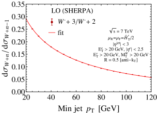
(a)	(b)
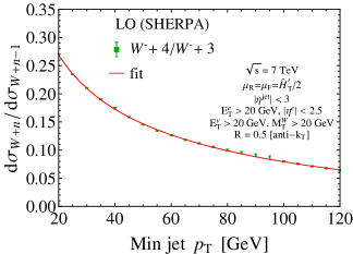
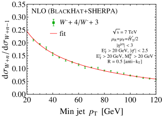
(c)	(d)
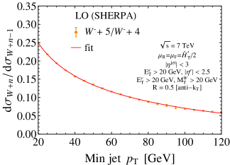
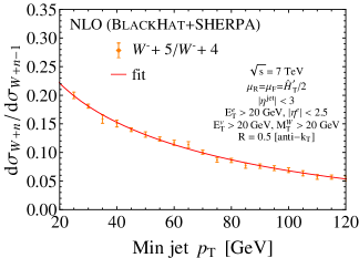
(e)	(f)

Figure 4: Fits to the ratio of the $W^{-}\,\!+\,n$-jet to $W^{-}\,\!+\,(n\!-\!1)$-jet cross sections as a function of the jet $p_{\rm T}^{\text{min}}$ cut. In the left column we show the ratios at LO and in the right column, at NLO. From top to bottom, $n$ goes from 3 to 5.

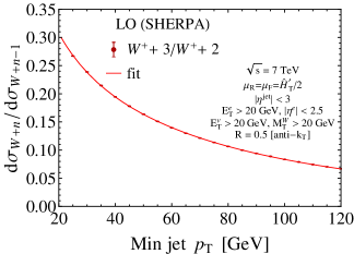
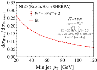
(a)	(b)
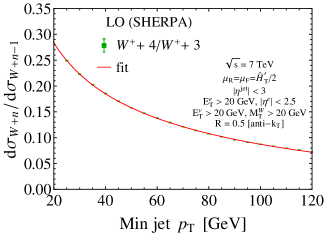
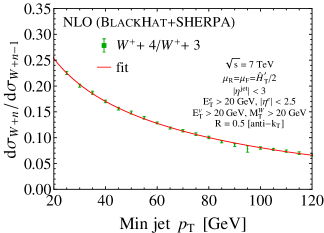
(c)	(d)
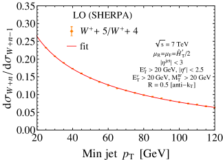
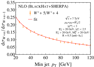
(e)	(f)

Figure 5: Fits to the ratio of the $W^{+}\,\!+\,n$-jet to $W^{+}\,\!+\,(n\!-\!1)$-jet cross sections as a function of the minimum jet $p_{\rm T}$ cut. In the left column we show the ratios at LO and in the right column, at NLO. From top to bottom, $n$ goes from 3 to 5.

The values of $d_{n}$ are not universal, but those for the primary exponent of interest $\eta_{n}$ are nearly independent of the number of jets, and also change very little in going from LO to NLO. We show the fits to the $W^{-}\,\!+\,3$-jet to $W^{-}\,\!+\,2$-jet, $W^{-}\,\!+\,4$-jet to $W^{-}\,\!+\,3$-jet, and $W^{-}\,\!+\,5$-jet to $W^{-}\,\!+\,4$-jet ratios in fig. 4, with the LO ratios in the left-hand column, and the NLO ratios in the right-hand column. The central value for the exponent in the $W^{-}\,\!+\,5$-jet to $W^{-}\,\!+\,4$-jet ratio is different, but the statistical uncertainty is large, and the result for $\eta_{n}$ remains marginally consistent with the other $\eta_{n}$s. We have not studied the sensitivity of this fit to the various cuts defining the sample, such as the cut on the lepton rapidity. The exponents are similar for $W^{+}\,\!+\,n$-jet production, for which we show the fits to the ratios in fig. 5.

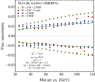
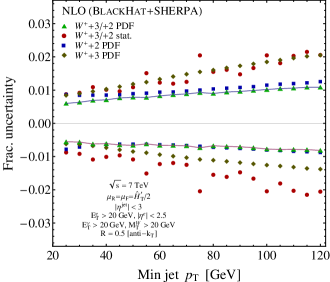
Figure 6: PDF uncertainties in $W\,\!+\,2$-jet and $W\,\!+\,3$-jet production at NLO as a function of the minimum jet transverse momentum cut $p_{\rm T}^{\text{min}}$. The plots show the PDF uncertainties on the $W\,\!+\,3$/$W\,\!+\,2$-jet ratio (green triangles joined by lines), the separate uncertainties on the $W\,\!+\,3$- (olive diamonds) and $W\,\!+\,2$-jet (dark blue squares) cross sections. The statistical uncertainty on the $W\,\!+\,3$/$W\,\!+\,2$-jet ratio (dark red circles) is also shown for comparison. The left plot shows the $W^{-}$ cross sections, and the right plot the $W^{+}$ ones.

As explained in the introduction, we save our results in an intermediate format which makes it straightforward and efficient to evaluate cross sections and distributions for PDF error sets NtuplesNote . We have made use of the $n$-tuples to evaluate the PDF uncertainties on the cross sections and on their ratios as a function of $p_{\rm T}^{\text{min}}$. To do so, we calculate the different $W\,\!+\,n$-jet cross sections, as well as their ratios, for each element of an MSTW PDF set, and use the standard weighting procedure to obtain 68% upper and lower confidence intervals. We display the results for $W\,\!+\,2$- and $W\,\!+\,3$-jet production, along with their ratio, in fig. 6. The figure shows that the PDF uncertainties are small, ranging from 0.5% for smaller values of $p_{\rm T}^{\text{min}}$ to just below 1% for the range of cuts we have studied. The PDF uncertainties on the ratio are slightly smaller than those on the $W\,\!+\,2$-jet cross section, and a factor of two smaller than those on the $W\,\!+\,3$-jet cross section. The PDF uncertainties on the ratio are comparable to the statistical uncertainties for $W^{-}\,\!+\,n$-jet production, and smaller than the statistical uncertainties for $W^{+}\,\!+\,n$-jet production, for the samples used in this study.

III.2 Dependence on the Vector Boson Transverse Momentum

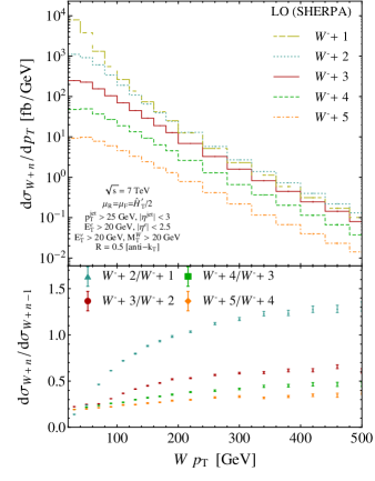
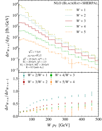
Figure 7: The LO and NLO vector-boson $p_{\rm T}$ distributions for $W^{-}\,\!+\,n$-jet production at the LHC. The upper panels show the distributions in fb/GeV: $W^{-}\,\!+\,1$-jet production through $W^{-}\,\!+\,5$-jet production are ordered from top to bottom. The thin vertical lines, where visible, indicate the statistical uncertainties. The lower panels show the jet-production ratios. The left plot are the distributions and ratios at LO, the right plot at NLO.

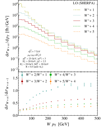
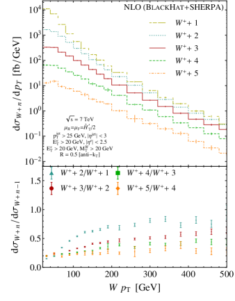
Figure 8: The LO and NLO vector-boson $p_{\rm T}$ distributions for $W^{+}\,\!+\,n$-jet production at the LHC. The upper panels show the distributions in fb/GeV: $W^{+}\,\!+\,1$-jet production through $W^{+}\,\!+\,5$-jet production are ordered from top to bottom. The lower panels show the jet-production ratios. The left plot shows the distributions and ratios at LO, the right plot at NLO.

We turn next to the dependence of the jet-production ratio on the $W$-boson transverse momentum. The dependence of jet-production ratios on the vector boson $p_{\rm T}$ was studied previously for jet production in association with $Z$ bosons at the Tevatron BlackHatZ3jet . We provide tables of the LO and NLO differential cross sections at the LHC as a function of the $W$ $p_{\rm T}$ in $W\,\!+\,1$-jet through $W\,\!+\,5$-jet production in appendix B. We display these differential cross sections in the upper panels of fig. 7 for the $W^{-}$, and of fig. 8 for the $W^{+}$.

The corresponding jet-production ratios are shown differentially in the $W$ $p_{\rm T}$ in the lower panels of these figures. In the lowest $p_{\rm T}$ bins, up to a $p_{\rm T}$ of order the $W$ mass, the ratio takes on a value near $0.25$, roughly independent of the number of jets, and the NLO corrections are modest. This is in agreement with the ratios of total cross sections that can be obtained from Table 1. In order to get a feeling for how well these ratios will continue to hold when cuts are tightened, e.g. a cut on ${{\raise 0.91666pt\hbox to7.95831pt{\hss/\hss}\hbox to0.0pt{\hss$E$}}}_{\rm T}$ in searches for new physics at ever-higher energy scales, we can examine their dependence on the vector-boson transverse momentum. Ref. BlackHatZ3jet already noted strong sensitivity of the jet-production ratios to the $Z$ boson’s $p_{\rm T}$ for $Z\,\!+\,n$-jet production at the Tevatron (at $\sqrt{s}=1.96$ TeV). This was especially true for the $Z\,\!+\,2$-jet to $Z\,\!+\,1$-jet ratio, but held for the $Z\,\!+\,3$-jet to $Z\,\!+\,2$-jet ratio as well.

Figs. 7 and 8 reveal that the seeming independence of the jet-production ratio from the number of jets is also misleading at the LHC. Once again, it holds only for vector-boson $p_{\rm T}$s of less than 60 GeV. At higher $p_{\rm T}$, the ratios change noticeably as the number of jets changes. Of course, if no cut is placed on the vector-boson $p_{\rm T}$, the bulk of the cross-section arises from lower $p_{\rm T}$, and the ratio of total cross sections will be insensitive to the number of jets. This insensitivity cannot be extrapolated safely to measurements with a large value of the cut on the $W^{\pm}$ $p_{\rm T}$. Furthermore, the ratios for $W\,\!+\,2$-jet/$W\,\!+\,1$-jet and $W\,\!+\,3$-jet/$W\,\!+\,2$-jet production show substantial NLO corrections. This is as expected, following the discussion in the previous subsection. The sensitivity of the ratios to the $W$ $p_{\rm T}$ decreases slowly with increasing number of jets, although it still remains noticeable for $W\,\!+\,5$-jet production. The NLO corrections are smaller beyond $W\,\!+\,2$ jets.

An approximate fit to these differential jet-production ratios was provided in ref. BlackHatZ3jet . The fit’s functional form was motivated by the expectation that at very large vector-boson transverse momentum $p_{\rm T}^{V}$, the matrix element would be maximized for an asymmetric configuration of jets, corresponding to a near-singular configuration of the partons. A typical configuration, for example, would have one hard jet recoiling against the vector boson, and additional jets (if any) with small transverse momenta just above the minimum jet transverse momentum. In these configurations, the short-distance matrix element will factorize into a matrix element for production of one hard gluon, and a singular factor (a splitting function in collinear limits, or an eikonal one in soft limits). The phase-space integrals over these near-singular configurations give rise to potentially large logarithms. Because the minimum jet–jet distance $R$ is relatively large, collinear logarithms should not play an important role; on the other hand, $p_{\rm T}^{V}/p_{\rm T}^{\text{min}}$ can become large (where $p_{\rm T}^{\text{min}}$ is the minimum jet $p_{\rm T}$), so its logarithm will play a role.

Process		Fit Values
		$N_{n}/N_{n-1}$	$c_{n}$	$\gamma_{n}$
$\displaystyle\quad{W^{-}+2}\quad$	LO	$2.50\pm 0.06$	$-0.36\pm 0.03$	$0.1\pm 0.2$
	NLO	$1.75\pm 0.05$	$-0.15\pm 0.04$	—
$\displaystyle\quad{W^{-}+3}\quad$	LO	$1.32\pm 0.03$	$-0.64\pm 0.03$	$1.0\pm 0.2$
	NLO	$1.36\pm 0.03$	$-0.52\pm 0.04$	—
$\displaystyle{W^{-}+4}$	LO	$0.80\pm 0.01$	$-0.74\pm 0.03$	—
	NLO	$0.83\pm 0.04$	$-0.6\pm 0.1$	—
$\displaystyle{W^{-}+5}$	LO	$0.56\pm 0.01$	$-0.66\pm 0.04$	—
	NLO	$0.50\pm 0.08$	$-0.2\pm 0.3$	—

Table 4: Fit parameters for the jet-production ratio in $W^{-}\,\!+\,n$ jets as a function of the $W$ $p_{\rm T}$, using the form in eq. (9). Dashes indicate parameters that are fixed as described in the text rather than fitted.

Process		Fit Values
		$N_{n}/N_{n-1}$	$c_{n}$	$\gamma_{n}$
$\displaystyle\quad{W^{+}+2}\quad$	LO	$2.6\pm 0.1$	$-0.38\pm 0.05$	$0.7\pm 0.3$
	NLO	$1.84\pm 0.07$	$-0.15\pm 0.06$	—
$\displaystyle\quad{W^{+}+3}\quad$	LO	$1.25\pm 0.02$	$-0.59\pm 0.02$	$0.9\pm 0.1$
	NLO	$1.22\pm 0.04$	$-0.38\pm 0.05$	—
$\displaystyle{W^{+}+4}$	LO	$0.799\pm 0.007$	$-0.64\pm 0.02$	—
	NLO	$0.87\pm 0.05$	$-0.5\pm 0.1$	—
$\displaystyle{W^{+}+5}$	LO	$0.58\pm 0.01$	$-0.53\pm 0.03$	—
	NLO	$0.46\pm 0.06$	$0.0\pm 0.3$	—

Table 5: Fit parameters for the jet-production ratio in $W^{+}\,\!+\,n$ jets as a function of the $W$ $p_{\rm T}$, using the form in eq. (9). Dashes indicate parameters that are fixed as described in the text rather than fitted.

The approximate factorization suggested the following model for differential cross sections,

$$\frac{d\sigma_{V+n}}{dp_{\rm T}^{V}}=(a_{s}(p_{\rm T}^{V}))^{n}f(p_{\rm T}^{V})\biggl{(}\sum_{j=0}^{n-1}{\bar{c}}^{(n)}_{j}\ln^{j}\rho\biggr{)}\bigl{(}1-p_{\rm T}^{V}/p_{\rm T}^{{\rm max}}\bigr{)}^{\gamma_{n}}\,,$$ (7)

where $\rho=p_{\rm T}^{V}/p_{\rm T}^{\text{min}}$, $p_{\rm T}^{{\rm max}}=3.5$ TeV is the maximum transverse momentum at $\sqrt{s}=7$ TeV, and where

$$a_{s}(p_{\rm T})\equiv\alpha_{s}(p_{\rm T})N_{c}/(2\pi)\,.$$ (8)

The last factor in eq. (7) takes into account the different phase-space limits and suppression due to parton distribution functions as a function of the number of jets $n$. It is of course much less important at the LHC than at the Tevatron. The function $f(p_{\rm T}^{V})$, which describes the overall, rapidly falling behavior of the distribution, will cancel in the ratios, leaving us with the parameters ${\bar{c}}^{(n)}_{j}$ and $\gamma_{n}$. The calculations we have performed, and especially their statistical errors, do not allow us to fit all the parameters in eq. (7) in a stable manner. Accordingly, we simplify the model, retaining only the two leading logarithms for each value of $n$; and retaining distinct exponents $\gamma_{n}$ only for $n=2,3$ at LO. We set the NLO $\gamma_{n}$s to be equal to their LO counterparts, and also set $\gamma_{5}=\gamma_{4}=\gamma_{3}$. We adopt a slightly different parametrization,

$$\frac{d\sigma_{V+n}}{dp_{\rm T}^{V}}=\big{(}4a_{s}(p_{\rm T}^{V})\big{)}^{n}f(p_{\rm T}^{V})N_{n}\bigl{(}\ln^{n-1}\rho+c_{n}\ln^{n-2}\rho\bigr{)}\bigl{(}1-p_{\rm T}^{V}/p_{\rm T}^{{\rm max}}\bigr{)}^{\gamma_{n}}\,,$$ (9)

where we omit the $\ln^{n-2}\rho$ term for $n=1$, and also set $N_{1}=1$ and $\gamma_{1}=0$. (Because the form of the factor in which $\gamma_{n}$ enters, the value of $\gamma_{1}$ has no significance for the ratio fits we perform; it will merely shift $\gamma_{n>1}$ by whatever amount to which it is set.) The fit quantities $N_{n}/N_{n-1}$, $c_{n}$, and $\gamma_{n}$ are dimensionless.

The distributions in figs. 7 and 8 have structure at $p_{\rm T}\lesssim M_{W}$, transitioning to a more uniform ‘scaling’ region at higher $p_{\rm T}$. The model in eq. (9) might be expected to provide adequate fits only far into this latter region, where $p_{\rm T}^{V}\gg M_{W}$ (so that mass effects are negligible), and where $p_{\rm T}^{V}\gg p_{\rm T}^{\text{min}}$ so that the logarithms will dominate over any finite terms. In practice, we find that the fits turn out to work well as far down as $p_{\rm T}^{V}$ of ${\cal O}(80$–100 GeV$)$ where $p_{\rm T}^{V}/p_{\rm T}^{\text{min}}\sim 3$ to 4.

Accordingly, we include essentially all calculated points in the expected scaling region with reasonable statistical errors: all bins with $80\leq p_{\rm T}^{V}\leq 500$ for $n=2,3$ and all bins with $100\leq p_{\rm T}^{V}\leq 500$ for $n=4,5$. We perform a nonlinear fit, numerically minimizing a goodness-of-fit function. We obtain stable fits for this simplified model, ranging from good to acceptable. In performing these fits, we first fit the form (9) to the computed $W\,\!+\,2$-jet to $W\,\!+\,1$-jet ratio, and then use the resulting fits for $N_{2}$ and $c_{2}$ in fitting eq. (9) to the $W\,\!+\,3$-jet to $W\,\!+\,2$-jet ratio, and so on. We obtain the fit parameters directly; the uncertainties we obtain using the Monte-Carlo procedure described in section III.1. As in the case of the $p_{\rm T}^{\text{min}}$-dependence of the total cross section discussed in the previous subsection, this model is not exact. Hence, as we increase the statistics in our calculation, we should expect the quality of the fit to deteriorate. For uncertainties of the magnitude of typical experimental errors, we expect the fits to describe the data very well. Although these distributions have fewer computed points to fit than the $p_{\rm T}^{\text{min}}$-dependent total cross section discussed in the previous section, it is still striking that the results can be parametrized so simply.

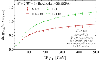
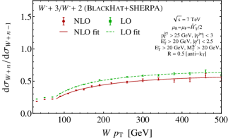
(a)	(b)
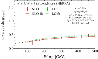
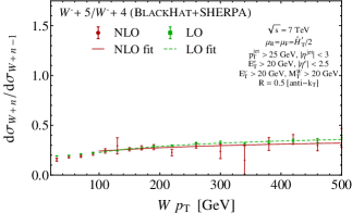
(c)	(d)

Figure 9: Fits to the ratios of the $W^{-}\,\!+\,n$-jet to $W^{-}\,\!+\,(n\!-\!1)$-jet differential cross sections as a function of the $W$ $p_{\rm T}$. Each plot shows the computed LO and NLO ratios, as well as fits with the parameters in table 4. In (a), (b), (c) and (d) the cases with $n=2,3,4,5$ are shown, respectively.

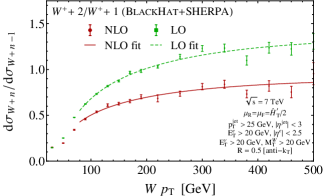
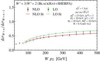
(a)	(b)
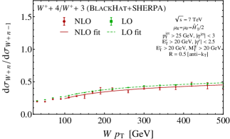
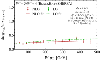
(c)	(d)

Figure 10: Fits to the ratios of the $W^{+}\,\!+\,n$-jet to $W^{+}\,\!+\,(n\!-\!1)$-jet differential cross sections as a function of the $W$ $p_{\rm T}$. Each plot shows the computed LO and NLO ratios, as well as fits with the parameters in table 5. In (a), (b), (c) and (d) the cases with $n=2,3,4,5$ are shown, respectively.

Our results for the $W^{-}$ fits are described in table 4, and those for $W^{+}$ in table 5. We display the $W^{-}$ fits in fig. 9, and the $W^{+}$ fits in fig. 10.

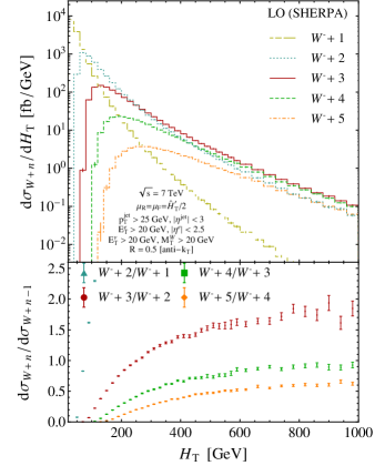
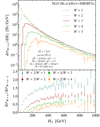
Figure 11: The LO and NLO $H_{\rm T}$ distributions for $W^{-}\,\!+\,n$-jet production at the LHC. The upper panels show the distributions in fb/GeV. From top to bottom, we display results for $W^{-}\,\!+\,1$-jet production through $W^{-}\,\!+\,5$-jet production. The lower panels show the jet-production ratios. The left plot shows the distributions and ratios at LO, the right plot at NLO.

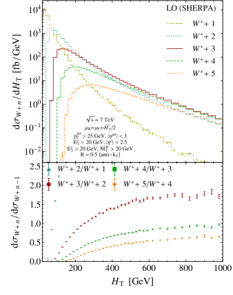
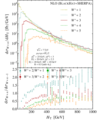
Figure 12: The LO and NLO $H_{\rm T}$ distributions for $W^{+}\,\!+\,n$-jet production at the LHC. The upper panels show the distributions in fb/GeV. From top to bottom, we display $W^{+}\,\!+\,1$-jet production through $W^{+}\,\!+\,5$-jet production. The lower panels show the jet-production ratios. The left plot shows the distributions and ratios at LO, the right plot at NLO.

III.3 Dependence on the Total Jet Transverse Energy

In this section, we study the dependence of the jet-production ratio on the total transverse energy in jets, $H_{\rm T}^{\rm jets}$, defined in eq. (2). In this section we denote it simply by $H_{\rm T}$. We provide tables of the LO and NLO differential cross sections as a function of $H_{\rm T}$ in $W\,\!+\,1$-jet through $W\,\!+\,5$-jet production in appendix C: the results for the LO differential cross section for $W^{-}\,\!+\,n$-jet production in table C, and the results for the NLO differential cross section in table LABEL:Wm-HTNLODistributionTable. The corresponding LO and NLO differential cross sections for $W^{+}\,\!+\,n$-jet production are shown in tables LABEL:Wp-HTLODistributionTable and LABEL:Wp-HTNLODistributionTable. These differential cross sections are also shown in the upper panels of fig. 11 for the $W^{-}$, and of fig. 12 for the $W^{+}$.

Each of these distributions rises from a threshold, passes through a peak, and then falls off at larger $H_{\rm T}$. The peak does not, of course, reflect any resonant behavior; it is a consequence of the small phase space available at the threshold of this distribution. As the number of jets grows, the minimum possible value of $H_{\rm T}$ also rises, and the peak of the distribution also shifts to higher values. Beyond roughly 300 GeV, all LO $W\,\!+\,n$-jet distributions for $n>1$ fall at similar rates. The LO distribution for $W\,\!+\,1$-jet production falls much faster. This rapid fall may seem odd, but has been understood by Rubin, Salam, and Sapeta RubinSalamSapeta . At LO, the $W$ boson is forced to have a large $p_{\rm T}$ at large $H_{\rm T}$, in order to balance the lone jet’s $p_{\rm T}$. At NLO, because we are studying the inclusive distribution, the leading jet’s $p_{\rm T}$ can be balanced by a second jet, and the $W$ boson can be much softer, leading to large double logarithms in $H_{\rm T}/M_{W}$. Thus the $W\,\!+\,1$-jet cross section increases dramatically at NLO, as seen in the plots on the right-hand side of figs. 11 and 12. This partially compensates the LO behavior, though the $W\,\!+\,1$ distribution still falls faster than distributions for $n\geq 2$ at the very highest values of $H_{\rm T}$.

The corresponding jet-production ratios are shown differentially in $H_{\rm T}$ in the lower panels of these figures. Although a factorization argument for this distribution is less compelling than for the $W$ $p_{\rm T}$ distribution, the success of the fits to the latter distribution down to relatively low $p_{\rm T}$, only just above $M_{W}$, suggests that we could try fitting to a form similar to that in eq. (9),

$$\frac{d\sigma_{V+n}}{dH_{\rm T}}=\big{(}2a_{s}(H_{\rm T}/2)\big{)}^{n}f^{H}(H_{\rm T})N^{H}_{n}\bigl{(}\ln^{n-1}\rho_{H,n}+c^{H}_{n}\ln^{n-2}\rho_{H,n}\bigr{)}\bigl{(}1-H_{\rm T}/H_{\rm T}^{\rm max}\bigr{)}^{\gamma^{H}_{n}}\,,$$ (10)

where $a_{s}$ is defined in eq. (8), $\rho_{H,n}=H_{\rm T}/(np_{\rm T}^{\text{min}})$, and $H_{\rm T}^{\rm max}\simeq 7$ TeV is the maximum total jet transverse energy (neglecting the effects of the $W$ transverse energy). Such a fit can be expected to work quite well at $H_{\rm T}$ values significantly above the peaks.

However, unlike the case of the $W$ $p_{\rm T}$ distribution, the thresholds for the distributions depend on $n$. This fact prevents the fit from being taken down to values just above the peak or at the peak, which would limit our ability to perform extrapolations using the fit forms.

Instead, let us proceed as follows. The threshold in the $H_{\rm T}$ distribution arises from the minimum jet $p_{\rm T}$; $H_{\rm T}$ cannot be less than $np_{\rm T}^{\text{min}}$ for $n$ jets. The phase-space integral near the threshold has the rough form,

$$\Big{[}\int\frac{dE}{E}\,g(E)\Big{]}^{n_{*}}\,,$$

where $n_{*}<n$, because not all jets can be soft, and where $g(E)$ is a slowly-varying function of the jet energy $E$. This suggests the following form for the threshold factor,

$$\ln^{\tau_{n}}\!\rho_{H,n}\,,$$ (11)

where $\tau_{n}$ is determined by a fit. The form of the phase-space constraints and the form of the parton distributions at large $x$ both suggest a large-$H_{\rm T}$ fall-off factor similar to that used earlier for fitting ratios of the $W$ $p_{\rm T}$ distribution,

$$\bigl{(}1-H_{\rm T}/H_{\rm T}^{\rm max}\bigr{)}^{\gamma_{n}^{H}}\,.$$ (12)

This leads us to use the following form for fits,

$$\frac{d\sigma_{V+n}}{dH_{\rm T}}=\big{(}2a_{s}(H_{\rm T}/2)\big{)}^{n}f^{H}(H_{\rm T})N^{H}_{n}\ln^{\tau^{H}_{n}}\!\rho_{H,n}\,\bigl{(}1-H_{\rm T}/H_{\rm T}^{\rm max}\bigr{)}^{\gamma^{H}_{n}}\,,$$ (13)

instead of the form in eq. (10). The remaining factor of $f^{H}(H_{\rm T})$ can be assumed to be $n$-independent for $n\geq 2$. We omit terms with additional subleading logarithms, as our results do not have the statistical precision to incisively determine their coefficients, and allowing them can lead some fits into unphysical regions for some parameters. The parameters $N^{H}_{n}$, $\gamma^{H}_{n}$, and $\tau^{H}_{n}$ are all dimensionless.

Process		Fit Values
		$N^{H}_{n}/N^{H}_{n-1}$	$\tau^{H}_{n}$	$\gamma^{H}_{n}$
$\displaystyle\quad{W^{-}+2}\quad$	LO	—	$0.75\pm 0.07$	—
	NLO	—	$1.1\pm 0.2$	—
$\displaystyle\quad{W^{-}+3}\quad$	LO	$8.5\pm 0.2$	$1.93\pm 0.04$	$6.3\pm 0.3$
	NLO	$7.7\pm 0.4$	$1.9\pm 0.1$	$5.0\pm 0.7$
$\displaystyle{W^{-}+4}$	LO	$6.46\pm 0.08$	$2.93\pm 0.02$	$8.0\pm 0.2$
	NLO	$6.7\pm 0.3$	$2.74\pm 0.05$	$7.2\pm 0.8$
$\displaystyle{W^{-}+5}$	LO	$5.3\pm 0.1$	$3.85\pm 0.02$	$9.5\pm 0.3$
	NLO	$6.2\pm 0.7$	$3.7\pm 0.1$	$11\pm 2$

Table 6: Fit parameters for the jet-production ratio in $W^{-}\,\!+\,n$ jets as a function of the jet $H_{\rm T}$, using the form in eq. (13). Dashes indicate parameters that are fixed as described in the text rather than fitted, or where we have not carried out a fit.

Process		Fit Values
		$N^{H}_{n}/N^{H}_{n-1}$	$\tau^{H}_{n}$	$\gamma^{H}_{n}$
$\displaystyle\quad{W^{+}+2}\quad$	LO	—	$0.70\pm 0.06$	—
	NLO	—	$0.8\pm 0.5$	—
$\displaystyle\quad{W^{+}+3}\quad$	LO	$8.5\pm 0.1$	$1.90\pm 0.03$	$6.4\pm 0.2$
	NLO	$7\pm 1$	$1.7\pm 0.3$	$7\pm 1$
$\displaystyle{W^{+}+4}$	LO	$6.51\pm 0.04$	$2.921\pm 0.006$	$8.3\pm 0.1$
	NLO	$6.5\pm 0.3$	$2.64\pm 0.06$	$9.4\pm 0.8$
$\displaystyle{W^{+}+5}$	LO	$5.41\pm 0.07$	$3.89\pm 0.02$	$10.0\pm 0.2$
	NLO	$5.0\pm 0.5$	$3.5\pm 0.1$	$10\pm 2$

Table 7: Fit parameters for the jet-production ratio in $W^{+}\,\!+\,n$ jets as a function of the jet $H_{\rm T}$, using the form in eq. (13). Dashes indicate parameters that are fixed as described in the text rather than fitted, or where we have not carried out a fit.

Because we have computed the $H_{\rm T}$ distribution out to larger values than the $W$ $p_{\rm T}$ distribution, the effect of the large-$H_{\rm T}$ suppression factor is more noticeable. The different behavior of the $W\,\!+\,1$-jet distribution at LO, as discussed above, makes it unsuitable for the same fit. Therefore we drop it, and do not fit the LO $W\,\!+\,2$-jet to $W\,\!+\,1$-jet ratio. Instead, we set $N^{H}_{2}=1$. We start fitting with the $W\,\!+\,3$-jet to $W\,\!+\,2$-jet ratio, where in addition to $N^{H}_{3}$, $\tau^{H}_{3}$, and $\gamma^{H}_{3}$, we also fit for $\tau^{H}_{2}$. We set $\gamma^{H}_{2}=17/4$, which is approximately the value we would obtain from an NLO fit to the $W\,\!+\,2$-jet to $W\,\!+\,1$-jet ratio with $\gamma^{H}_{1}=0$. We then use these values in fitting the ratio of forms in eq. (13) to the $W\,\!+\,4$-jet to $W\,\!+\,3$-jet ratio in order to determine $N^{H}_{4}$, $\tau^{H}_{4}$, and $\gamma^{H}_{4}$, and so on. We repeat this procedure at NLO, starting again with the $W\,\!+\,3$-jet to $W\,\!+\,2$-jet ratio. In all the fits, we drop the bin nearest threshold, but otherwise include all bins up to $1000$ GeV. (The bin sizes are larger for larger $H_{\rm T}$, as shown in tables C–LABEL:Wp-HTNLODistributionTable.) We perform a nonlinear fit, and obtain fit parameters directly, and the uncertainties using the Monte-Carlo procedure described in section III.1. We obtain fits that range from marginally adequate (probabilities of 1–2%) to adequate (probabilities of $\gtrsim 10$%). The results of the fits are shown in table 6 for jet production in association with a $W^{-}$ boson, and in table 7 for production in association with a $W^{+}$ boson.

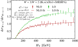
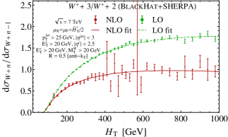
(a)	(b)
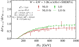
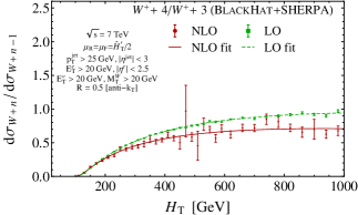
(c)	(d)
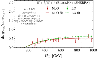
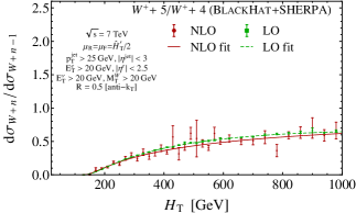
(e)	(f)

Figure 13: Fits to the ratios of the $W\,\!+\,n$-jet to $W\!+\,(n\!-\!1)$-jet differential cross sections as a function of $H_{\rm T}$. Each plot shows the computed LO and NLO ratios, as well as fits with the parameters in tables 6 and 7. In the left column we show the ratios for $W^{-}$ and in the right column for $W^{+}$. From top to bottom, $n$ goes from 3 to 5.

We display these fits to the jet production ratios in fig. 13. The same remarks apply here as in fits to the total cross sections as functions of the minimum jet $p_{\rm T}$, and to the differential cross sections in the $W$ boson $p_{\rm T}$: the functional forms are only approximate, and the adequacy of the fits reflects the limited statistical precision of our Monte-Carlo integrations. Nonetheless, it is remarkable that the results can be fit with so few parameters, and fits to experimental data should be expected to be quite good, given anticipated experimental uncertainties.

In our study of $W\,\!+\,5$-jet production W5j , we used the results for the NLO total cross sections for $W\,\!+\,3$-jet, $W\,\!+\,4$-jet, and $W\,\!+\,5$-jet production to extrapolate and obtain predictions for the total cross sections at NLO for $W^{-}\,\!+\,6$-jet and $W^{+}\,\!+\,6$-jet production. Here, we will go a bit further, and extrapolate to obtain a prediction for the $H_{\rm T}$ differential cross section in $W\,\!+\,6$-jet production at NLO.

We will use the form in eq. (13), and extrapolate the NLO parameters in tables 6 and 7. Because of the different behavior of the $W\,\!+\,2$-jet to $W\,\!+\,1$-jet ratio, we exclude it from the fit. We perform a linear extrapolation on the $\tau^{H}_{n}$ and $\gamma^{H}_{n}$, and determine $N^{H}_{6}$ by matching to the extrapolated total cross section rather than by direct extrapolation of the ratios in tables 6 and 7. This gives us a prediction for the ratio of $H_{\rm T}$ distributions in $W\,\!+\,6$-jet and $W\,\!+\,5$-jet production. In order to obtain an estimate of an uncertainty band for this prediction, we again use a Monte Carlo approach. Because the uncertainties on the $\tau^{H}$s and $\gamma^{H}$s are highly correlated, we estimate the uncertainties in the extrapolation as follows.

We generate an ensemble of 1,000 synthetic data sets, where each bin of the different $H_{\rm T}$ distributions is chosen from a normally-distributed ensemble with mean given by the computed value, and width given by the estimated statistical uncertainty in our NLO computation. For each collection of distributions from the ensemble, we form the $W\,\!+\,n$- to $W\!+\,(n\!-\!1)$-jet ratios, and fit to ratios of the corresponding forms from eq. (13). We also compute the corresponding total cross section by summing all bins. For each collection, we then extrapolate the total cross section as well as the $\tau^{H}_{n}$ and $\gamma^{H}_{n}$ parameters linearly. That is, we perform the entire fitting and extrapolation procedure independently for each synthetic data set. This provides us with an element of an ensemble of curves around our central prediction. For our uncertainty band, we retain all curves whose parameters are within the correlated 68% confidence-level ellipsoid of the central values of the fits. In the present case, the parameters are highly correlated; ignoring the correlations would yield a much wider uncertainty band.

In order to extrapolate the distributions (and not just ratios of distributions), we need to have an estimate of the $f^{H}$ function appearing in eq. (13). To obtain one, we make use of the $W\,\!+\,2$-jet differential distribution,

$$f^{H}(H)\stackrel{{\scriptstyle\rm est}}{{=}}\frac{d\sigma_{W+2}}{dH_{\rm T}}(H)(2a_{s}(H/2))^{-2}(N_{2}^{H})^{-1}\ln^{-\tau^{H}_{2}}\!\rho_{H}\,\bigl{(}1-H/H_{\rm T}^{\rm max}\bigr{)}^{-\gamma^{H}_{2}}\,.$$ (14)

One could imagine using this equation to obtain values for $f^{H}(H)$ point-by-point, but it turns out to be more convenient and more stable to have an analytic form for it. In order to obtain such a form, we need a fit to the $W\,\!+\,2$-jet NLO differential cross section. It turns out that we can use the following form to fit $f^{H}(H)$,

$$g_{2}\ln^{r}(H/10)\biggl{(}\frac{H}{2p_{\rm T}^{\text{min}}}\biggr{)}^{\omega_{2}}e^{-h_{*}H}\,,$$ (15)

and obtain an adequate fit. The parameters are,

$$g_{2}=100{}^{+339}_{-77}\cdot 10^{3}\,,\quad\omega_{2}=-4.2\pm 0.7\,,\quad h_{*}=0.0025\pm 0.0004\,,\quad r=3\pm 2\,,$$ (16)

for $W^{-}$ and,

$$g_{2}=17{}^{+328}_{-16}\cdot 10^{3}\,,\quad\omega_{2}=-5\pm 1\,,\quad h_{*}=0.0016\pm 0.0008\,,\quad r=6\pm 4\,,$$ (17)

for $W^{+}$. (The distribution for $g_{2}$ is log-Gaussian rather than Gaussian. The uncertainties on it are much larger than the statistical uncertainty on the total cross section, because it is strongly correlated with the other parameters. Two of the parameters, $\omega_{2}$ and $r$, are dimensionless; $g_{2}$ has units of fb/GeV, and $h_{*}$ of GeV^-1.)

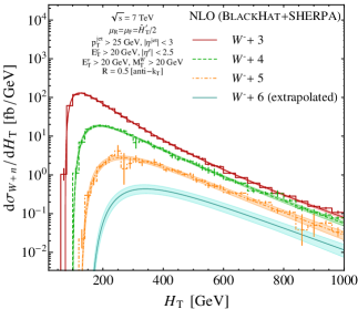
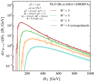
Figure 14: NLO predictions for $H_{\rm T}$ distributions for $W\,\!+\,n$-jet production at the LHC, based on fits to ratios of distributions, along with an extrapolation for $n=6$. The computed numerical distributions for $n=3,4,5$ are shown against the predictions based on direct fits to ratios of distributions. From the top down, the curves (dark red, green, and orange) correspond to $n=3,4,5$. The extrapolation-based prediction for $n=6$ is the bottom distribution, shown in a solid (turquoise) line, with a shaded (light turquoise) band showing the statistical uncertainty in our prediction. The normalizations of the curves are adjusted to the total cross sections given in table 1 for $W\,\!+\,3$ through $W\,\!+\,5$-jet W5j , and to the extrapolated total cross section for $W\,\!+\,6$-jet. The left plot is for $W^{-}$, and the right plot for $W^{+}$.

We can verify the consistency of this procedure, by comparing the total cross sections for $n=3,4,5$ obtained by integrating the ‘predicted’ differential cross sections over the entire range from threshold to the maximum $H_{\rm T}$ with the corresponding NLO total cross sections computed by summing the $H_{\rm T}$ histograms. We find that they are in agreement. After extrapolating the exponents in eq. (13), and fixing the normalization $N^{H}_{6}$ using the extrapolated value of the total cross section W5j ,

$$W^{-}+6\hbox{ jets}:\quad 0.15\pm 0.01\ \hbox{pb}\,,$$

$$W^{+}+6\hbox{ jets}:\quad 0.30\pm 0.03\ \hbox{pb}\,,$$ (18)

we find for $W^{-}$,

$$N^{H}_{6}=2.0\cdot 10^{3}\,,\quad\tau^{H}_{6}=4.6\pm 0.1\,,\quad\gamma^{H}_{6}=13\pm 2\,,$$ (19)

and for $W^{+}$,

$$N^{H}_{6}=1.0\cdot 10^{3}\,,\quad\tau^{H}_{6}=4.3\pm 0.2\,,\quad\gamma^{H}_{6}=11\pm 3\,.$$ (20)

We do not quote an error for the normalization $N^{H}_{6}$ because its value is tightly correlated with the values of the exponents. The predictions for the $W\,\!+\,6$-jet $H_{\rm T}$ distributions are shown in fig. 14.

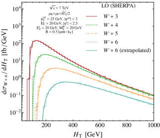
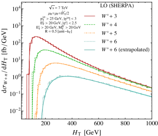
Figure 15: LO test of an extrapolation to $W\,\!+\,6$ jets. The $H_{\rm T}$ distributions for $W\,\!+\,n$-jet production at the LHC are computed at LO for $n=3,4,5,6$ (histograms). The predictions based on fits to ratios of LO distributions are the curves, from the top down (dark red, green, and orange) corresponding to $n=3,4,5$. The extrapolation-based prediction for $n=6$ is the bottom curve, shown as a solid (turquoise) line, with a shaded (light turquoise) band showing the statistical uncertainty in our prediction. The histogram shows a direct computation of the same distribution. The normalizations of the curves are adjusted, respectively, to the total cross sections given in table 1 for $W\,\!+\,3$ through $W\,\!+\,5$-jet, and to the extrapolated total cross section for $W\,\!+\,6$-jet. The left plot is for $W^{-}$, and the right plot for $W^{+}$.

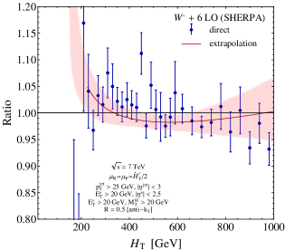
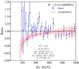
Figure 16: The ratio of the extrapolation-based LO prediction for the $H_{\rm T}$ distribution for $W\,\!+\,6$-jet production at the LHC to a fit to the direct computation (solid dark red line), along with a 68% uncertainty band for the extrapolation. The (blue) points show the ratio of the direct computation to a fit to that computation, with statistical uncertainties alone. The left plot is for $W^{-}$, and the right plot for $W^{+}$.

We can also check the extrapolation procedure described above by comparing an extrapolation against a direct calculation at LO. We have done this for the LO $W\,\!+\,6$-jet $H_{\rm T}$ distribution, where the direct calculation is feasible. The results are shown in fig. 15. The direct fit is again made by fitting ratios of the model in eq. (13) to the computed $W\,\!+\,6$-jet to $W\,\!+\,5$-jet ratio, and using the parameters obtained, along with those in eqs. (16) and (17), to obtain a curve for the $W\,\!+\,6$-jet $H_{\rm T}$ distribution itself. The agreement of the extrapolation with the direct calculation is excellent. On a logarithmic scale, any differences are hard to see, so in fig. 16 we show the ratios of the extrapolated distribution and of the computed distributions to the direct fit to the computation. The direct fit in this figure is thus represented by the horizontal axis; the computation by itself by the points with associated statistical uncertainties and the extrapolated distribution by the colored curve. The uncertainty in the extrapolation is given by the shaded band. For $W^{-}$ production, the extrapolation, direct fit, and calculation all agree within 5% except right above threshold. In the region contributing the bulk of the cross section, the extrapolation and direct fit agree within 3%. For $W^{+}$ production, the agreement is not as good, but the extrapolation, direct fit, and calculation again agree to within 5% over most of the range.

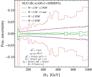
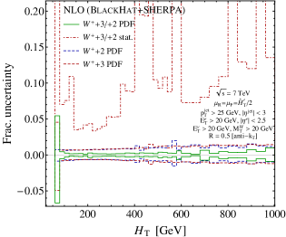
Figure 17: PDF uncertainties in the ratio of the $W\,\!+\,3$-jet to $W\,\!+\,2$-jet $H_{\rm T}$ distribution at NLO. The plots show, from the smallest absolute values to the largest: the PDF uncertainties on the $W\,\!+\,3$/$W\,\!+\,2$-jet ratio (solid green); the separate uncertainties on the $W\,\!+\,3$- (dashed dark red) and $W\,\!+\,2$-jet (dashed blue) distributions; and the statistical uncertainty on the $W\,\!+\,3$/$W\,\!+\,2$-jet ratio (dot-dashed dark red) shown for comparison. The left plot shows the $W^{-}$ differential cross sections, and the right plot the $W^{+}$ ones. In the right plot, only the positive statistical uncertainty is shown.

We have also evaluated the PDF uncertainties for the $H_{\rm T}$ distribution, using the same approach as for the total cross sections studied in section III.1. We display the results in fig. 17. The left figure shows that the PDF uncertainties in the separate $W^{-}\,\!+\,2$-jet and $W^{-}\,\!+\,3$-jet distributions are small, ranging from 1% at smaller values of $H_{\rm T}$ above the $W\,\!+\,3$-jet threshold to just below 3% at the highest values. The PDF uncertainties in the ratio are considerably smaller, ranging from 0.5% at smaller $H_{\rm T}$ values to less than 1% even at the highest $H_{\rm T}$ values. In $W^{+}\,\!+\,n$-jet production, the PDF uncertainties on the separate distributions are smaller than in the $W^{-}\,\!+\,n$-jet case, but the uncertainties on the ratios remain comparably smaller. With the number of events we have collected, these uncertainties are considerably smaller than the statistical uncertainties in the ratio, especially in $W^{+}\,\!+\,n$-jet production.

III.4 Dependence on Jet Transverse Momenta

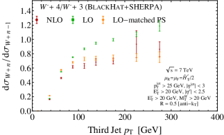
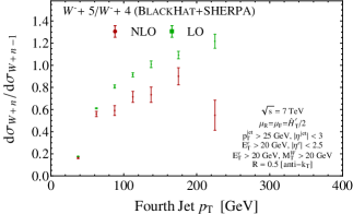
(a)	(b)

Figure 18: The ratios of $W^{-}\,\!+\,n$-jet to $W^{-}\,\!+\,(n\!-\!1)$-jet cross sections as a function of the softest-jet $p_{\rm T}$, at LO, at NLO, and for the $W^{-}\,\!+\,4$-jet to $W^{-}\,\!+\,3$-jet ratio, in a parton-shower calculation matched to LO. In (a) we show the $W^{-}\,\!+\,4$-jet to $W^{-}\,\!+\,3$-jet ratio as a function of the third-jet $p_{\rm T}$; and in (b) the $W^{-}\,\!+\,5$-jet to $W^{-}\,\!+\,4$-jet ratio as a function of the fourth-jet $p_{\rm T}$.

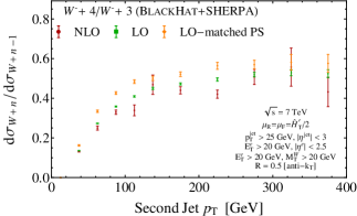
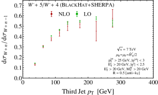
(a)	(b)

Figure 19: The ratios of $W^{-}\,\!+\,n$-jet to $W^{-}\,\!+\,(n\!-\!1)$-jet cross sections as a function of the next-to-softest-jet $p_{\rm T}$, at LO, at NLO, and for the $W^{-}\,\!+\,4$-jet to $W^{-}\,\!+\,3$-jet ratio, in a parton-shower calculation matched to LO. In (a) we show the $W^{-}\,\!+\,4$-jet to $W^{-}\,\!+\,3$-jet ratio as a function of the second-jet $p_{\rm T}$; and in (b) the $W^{-}\,\!+\,5$-jet to $W^{-}\,\!+\,4$-jet ratio as a function of the third-jet $p_{\rm T}$.

In this subsection, we study jet-production ratios as a function of various jet transverse momenta. We give detailed results for the LO and NLO $W^{-}\,\!+\,n$-jet differential cross section as a function of the second-, third-, and fourth-hardest jets’ transverse momenta in appendix LABEL:JetpTAppendix. We display jet-production ratios as functions of these jet transverse momenta in figs. 18 and 19, organized not by the ordinal jet number (as in appendix LABEL:JetpTAppendix), but rather according to whether the jet is the softest (ordered $n-1$) in the $W^{-}\,\!+\,(n\!-\!1)$-jet process, or the next-to-softest (ordered $n-2$). That is, we consider the ratios,

$$\frac{d\sigma^{W+n}/dp_{{\rm T},n-1}}{d\sigma^{W+n-1}/dp_{{\rm T},n-1}}{\hskip 8.5359pt\rm\ and\ \hskip 8.5359pt}\frac{d\sigma^{W+n}/dp_{{\rm T},n-2}}{d\sigma^{W+n-1}/dp_{{\rm T},n-2}}\,,$$ (21)

in figs. 18 and 19, respectively.

We see that the jet-production ratio as a function of the softest jet’s $p_{\rm T}$ (fig. 18) suffers large NLO corrections, whereas the corrections as a function of harder jet $p_{\rm T}$s (fig. 19) are much more modest. This is consistent with previous results W4j . For comparison, we also show results for the $W\,\!+\,4$-jet to $W\,\!+\,3$-jet ratio obtained using the SHERPA parton shower matched to LO. The parton-shower result is somewhat above the LO and NLO results for the next-to-softest jet, but in rough agreement with both. It is closer to the NLO result for the softest-jet distribution, suggesting that corrections beyond NLO are not large.

IV Conclusions

The first years of data and analyses from experiments at the Large Hadron Collider (LHC) emphasize the need for reliable theoretical calculations in searches for new physics beyond the Standard Model. In many channels, new-physics signals can hide in broad distributions underneath Standard Model backgrounds. Extraction of signals requires accurate predictions for the background processes, for which next-to-leading order (NLO) cross sections in perturbative QCD are an important first step.

In this paper, we computed jet-production ratios to NLO in QCD for $W$ production in association with up to five jets. Ratios of cross sections and of distributions are expected to have reduced theoretical and experimental uncertainties, most notably a reduced uncertainty in the jet-energy scale. The $W\,\!+\,n$- to $W\!+\,(n\!-\!1)$-jet ratios are formally of ${\cal O}(\alpha_{s})$, and accordingly are expected to have a much smaller scale dependence than the scale dependence of the underlying cross sections. We used a leading-color approximation for the virtual terms in $W\,\!+\,4$- and $W\,\!+\,5$-jet production. We had previously validated this approximation for $W\,\!+\,3$- and $W\,\!+\,4$-jet production W3jDistributions ; ItaOzeren . We expect the subleading-color terms to contribute less than 3% of the total cross section, though it would be useful to verify this for $W\,\!+\,5$-jet production. We expect other approximations we have used, such as neglecting real and virtual top-quarks, as well as real-emission contributions with four quark pairs, to have even smaller effects.

We have studied a number of quantities constructed from ratios of cross sections. In section III.1, we studied the ratio of cross sections as a function of the minimum jet transverse momentum $p_{\rm T}^{\text{min}}$. We saw that for ratios with $n\geq 3$, the dependence is quite similar for different values of $n$ even at LO, and very similar at NLO. This suggests a universal behavior that is in accord with the (weak) linear dependence on $n$ of ratios of total cross sections at fixed $p_{\rm T}^{\text{min}}$ W5j . The dependence on $p_{\rm T}^{\text{min}}$ can be described very well by a three-parameter functional form. Its behavior is dominated by a power-law behavior with an exponent consistent with being independent of the number of jets, both at LO and at NLO. We have studied the uncertainty on the ratios due to imprecise knowledge of the parton distribution functions, and find that as expected, the ratio is less sensitive than the underlying cross sections. For the range of $p_{\rm T}^{\text{min}}$ values we have studied (25 to 120 GeV), the fractional uncertainty in the ratio due to PDF uncertainty varies from 0.6% to 1.5%.

We have also studied more differential quantities. In section III.2, we studied ratios of differential distributions with respect to the transverse momentum of the $W$ boson $p_{\rm T}^{V}$. The ratios of distributions can be described by a simple three-parameter fit form, a simpler form than needed for the distributions themselves. The $W\,\!+\,2$- to $W\,\!+\,1$-jet ratio again behaves differently than ratios for $n\geq 3$; but the latter ratios are similar in shape, and depend primarily on powers of a single log of $p_{\rm T}^{V}/p_{\rm T}^{\text{min}}$. The simplicity of the ratios suggests that at large $p_{\rm T}^{V}$, the production process can be understood as the production of a $W$ boson recoiling against a jet system, with a universal function describing the “fragmentation” (perturbative splitting) of the jet system into individual jets. The NLO corrections are significant for $n=2$, but small for larger $n$.

In section III.3, we studied the ratios of differential distributions with respect to the total transverse energy in jets, $H_{\rm T}^{\rm jets}$. We again find that the ratios can be described in terms of a simple three-parameter fit function, with a universal function describing the production of the $W$-boson plus jet system dropping out of ratios. The parameters of these fit function for $n\geq 3$ are in turn very well described by a linear fit form. We have used this observation to extrapolate the $H_{\rm T}^{\rm jets}$ distribution to $W\,\!+\,6$-jet production at NLO. A similar extrapolation at LO agrees very nicely with a direct calculation, suggesting the procedure adds only 5% uncertainty over much of the range to the scale uncertainty. We expect that other distributions can be extrapolated using a similar approach.

Finally, in section III.4, we studied the ratios of differential distributions in jet transverse momenta. These ratios have large NLO corrections for the softest identified jet, but only modest corrections for harder jets. A comparison to parton shower results suggests that corrections beyond NLO are modest.

The study of extrapolations in section III.3 is motivated by the increasing difficulty of precision QCD calculations as the number of jets increases. The availability of the $W\,\!+\,5$-jet calculation was critical in allowing us to extrapolate to $W\,\!+\,6$-jet production, and in principle, beyond it. We look forward to comparing the quantities studied here, and extrapolations of this type, to LHC data.

Appendix A Cross Sections as a Function of the Minimum Jet Transverse Momentum

Min jet $p_{T}$	$\displaystyle\vphantom{\sum_{i=1}^{W}}\frac{W^{-}+2}{W^{-}+1}$	$\displaystyle\frac{W^{-}+3}{W^{-}+2}$	$\displaystyle\frac{W^{-}+4}{W^{-}+3}$	$\displaystyle\frac{W^{-}+5}{W^{-}+4}$
25	$0.2949(0.0004)$	$0.2511(0.0005)$	$0.2345(0.0009)$	$0.218(0.001)$
30	$0.2751(0.0003)$	$0.2222(0.0005)$	$0.2101(0.0009)$	$0.194(0.001)$
35	$0.2627(0.0004)$	$0.1988(0.0005)$	$0.190(0.001)$	$0.174(0.001)$
40	$0.2560(0.0004)$	$0.1795(0.0005)$	$0.175(0.001)$	$0.157(0.001)$
45	$0.2529(0.0004)$	$0.1635(0.0005)$	$0.159(0.001)$	$0.146(0.001)$
50	$0.2527(0.0005)$	$0.1498(0.0005)$	$0.1453(0.0009)$	$0.136(0.001)$
55	$0.2545(0.0005)$	$0.1379(0.0005)$	$0.134(0.001)$	$0.125(0.001)$
60	$0.2572(0.0005)$	$0.1266(0.0005)$	$0.126(0.001)$	$0.116(0.001)$
65	$0.2599(0.0006)$	$0.1166(0.0004)$	$0.118(0.001)$	$0.109(0.001)$
70	$0.2620(0.0006)$	$0.1078(0.0004)$	$0.112(0.001)$	$0.101(0.001)$
75	$0.2643(0.0007)$	$0.1008(0.0005)$	$0.106(0.001)$	$0.094(0.002)$
80	$0.2669(0.0007)$	$0.0938(0.0004)$	$0.100(0.002)$	$0.088(0.002)$
85	$0.2702(0.0008)$	$0.0875(0.0004)$	$0.096(0.002)$	$0.082(0.002)$
90	$0.2730(0.0008)$	$0.0823(0.0004)$	$0.091(0.002)$	$0.078(0.003)$
95	$0.2764(0.0009)$	$0.0773(0.0004)$	$0.087(0.003)$	$0.072(0.003)$
100	$0.280(0.001)$	$0.0731(0.0004)$	$0.080(0.001)$	$0.069(0.001)$
105	$0.284(0.001)$	$0.0691(0.0004)$	$0.076(0.001)$	$0.066(0.001)$
110	$0.288(0.001)$	$0.0651(0.0005)$	$0.071(0.001)$	$0.064(0.001)$
115	$0.292(0.001)$	$0.0614(0.0005)$	$0.068(0.001)$	$0.061(0.002)$
120	$0.296(0.001)$	$0.0581(0.0005)$	$0.064(0.001)$	$0.059(0.002)$

Table 8: The jet-production ratio in $W^{-}\,\!+\,n$ jets at LO as a function of the minimum jet $p_{\rm T}$ in GeV. These values are shown in the left plot in fig. 1.

Table 9: The jet-production ratio in $W^{+}\,\!+\,n$ jets at LO, as a function of the minimum jet $p_{\rm T}$ in GeV. These values are shown in the left plot in fig. 2.

Table 10: The jet-production ratio in $W^{-}\,\!+\,n$ jets at NLO, as a function of the minimum jet $p_{\rm T}$ in GeV. These values are shown in the right plot in fig. 1.

Table 11: The jet-production ratio in $W^{+}\,\!+\,n$ jets at NLO, as a function of the minimum jet $p_{\rm T}$ in GeV. These values are shown in the right plot in fig. 2.

In this appendix, we present the detailed results at LO and at NLO, for the ratio of $W\,\!+\,n$-jet to $W\!+\,(n\!-\!1)$-jet production when varying the cut on the minimum jet transverse energy across a range of values from 25 to 120 GeV. Our results for the ratio $W^{-}\,\!+\,n$-jet to $W^{-}\,\!+\,(n\!-\!1)$-jet production are given in tables A and A, and the results for the ratio of $W^{+}\,\!+\,n$-jet to $W^{+}\,\!+\,(n\!-\!1)$-jet production in tables A and A. We show corresponding numerical integration errors in parentheses.

Appendix B Differential Cross Sections as a Function of the $W$ Transverse Momentum

Table 12: The LO $W^{-}\,\!+\,n$-jet cross section taken differentially in the $W^{-}$ $p_{\rm T}$, in fb/GeV. These values are shown in the upper panel of the left figure in fig. 7.

Table 13: The NLO $W^{-}\,\!+\,n$-jet cross section taken differentially in the $W^{-}$ $p_{\rm T}$, in fb/GeV. These values are shown in the upper panel of the right figure in fig. 7.

Table 14: The LO $W^{+}\,\!+\,n$-jet cross section taken differentially in the $W^{+}$ $p_{\rm T}$, in fb/GeV. These values are shown in the upper panel of the left figure in fig. 8.

Table 15: The NLO $W^{+}\,\!+\,n$-jet cross section taken differentially in the $W^{+}$ $p_{\rm T}$, in fb/GeV. These values are shown in the upper panel of the right figure in fig. 8.

In this appendix, we present the detailed results at LO and at NLO for the cross section for $W\,\!+\,n$-jet production taken differentially in the $W$’s transverse momentum. We give the LO differential cross sections for $W^{-}\,\!+\,1$-jet through $W^{-}\,\!+\,5$-jet production in table A, and the corresponding results for the NLO differential cross section in table A. We give the LO and NLO differential cross sections for $W^{+}\,\!+\,1$-jet through $W^{+}\,\!+\,5$-jet production in tables A and A respectively. We show corresponding numerical integration errors in parentheses.

Appendix C Differential Cross Sections as a Function of the Total Jet Transverse Energy

$H_{\rm T}$	$W^{-}\,\!+\,1$	$W^{-}\,\!+\,2$	$W^{-}\,\!+\,3$	$W^{-}\,\!+\,4$	$W^{-}\,\!+\,5$
30	$7919(7)$	—	—	—	—
50	$3827(4)$	$294(2)$	—	—	—
70	$1319(2)$	$1093(3)$	$0.89(0.09)$	—	—
90	$552(1)$	$893(2)$	$62.6(0.7)$	—	—
110	$263.0(0.8)$	$604(2)$	$135.1(0.8)$	$1.2(0.2)$	—
130	$136.4(0.5)$	$395(1)$	$149.9(0.8)$	$8.6(0.2)$	$0.02(0.01)$
150	$73.6(0.3)$	$263.9(0.9)$	$134.7(0.6)$	$16.9(0.3)$	$0.31(0.04)$
170	$42.3(0.3)$	$177.5(0.7)$	$112.6(0.5)$	$21.8(0.3)$	$1.01(0.03)$
190	$25.0(0.2)$	$122.1(0.5)$	$91.3(0.5)$	$23.1(0.3)$	$2.04(0.07)$
210	$15.4(0.1)$	$85.4(0.4)$	$72.2(0.4)$	$22.3(0.3)$	$2.80(0.04)$
230	$9.61(0.09)$	$62.1(0.4)$	$57.3(0.4)$	$20.7(0.2)$	$3.42(0.05)$
250	$6.23(0.07)$	$45.6(0.3)$	$45.1(0.3)$	$18.6(0.2)$	$3.71(0.05)$
270	$4.07(0.05)$	$33.7(0.2)$	$35.3(0.2)$	$16.4(0.2)$	$3.70(0.04)$
290	$2.71(0.04)$	$24.8(0.2)$	$28.2(0.2)$	$14.2(0.2)$	$3.69(0.05)$
310	$1.91(0.04)$	$18.9(0.2)$	$22.6(0.2)$	$12.0(0.2)$	$3.46(0.04)$
330	$1.33(0.03)$	$14.6(0.1)$	$18.2(0.2)$	$10.1(0.1)$	$3.22(0.03)$
350	$0.93(0.02)$	$11.2(0.1)$	$14.4(0.1)$	$8.8(0.1)$	$2.97(0.03)$
370	$0.69(0.02)$	$9.1(0.1)$	$11.8(0.1)$	$7.31(0.09)$	$2.71(0.03)$
390	$0.49(0.01)$	$6.95(0.08)$	$9.61(0.09)$	$6.5(0.1)$	$2.42(0.03)$
410	$0.37(0.01)$	$5.71(0.09)$	$7.99(0.09)$	$5.29(0.07)$	$2.11(0.02)$
430	$0.256(0.008)$	$4.65(0.07)$	$6.49(0.07)$	$4.61(0.07)$	$1.94(0.03)$
450	$0.195(0.006)$	$3.74(0.06)$	$5.32(0.06)$	$3.80(0.05)$	$1.72(0.03)$
470	$0.147(0.005)$	$2.98(0.05)$	$4.44(0.05)$	$3.21(0.06)$	$1.46(0.02)$
490	$0.118(0.004)$	$2.47(0.04)$	$3.76(0.06)$	$2.81(0.08)$	$1.32(0.02)$
510	$0.083(0.003)$	$2.07(0.04)$	$3.25(0.06)$	$2.38(0.05)$	$1.13(0.01)$
530	$0.064(0.003)$	$1.71(0.03)$	$2.66(0.05)$	$2.03(0.04)$	$1.00(0.01)$
550	$0.049(0.002)$	$1.45(0.04)$	$2.28(0.05)$	$1.74(0.03)$	$0.89(0.01)$
570	$0.037(0.002)$	$1.21(0.03)$	$1.92(0.07)$	$1.52(0.03)$	$0.77(0.01)$
590	$0.030(0.002)$	$0.98(0.03)$	$1.59(0.03)$	$1.35(0.04)$	$0.70(0.01)$
620	$2.10(0.08)\cdot 10^{-2}$	$0.80(0.02)$	$1.28(0.02)$	$1.08(0.02)$	$0.569(0.007)$
660	$1.33(0.06)\cdot 10^{-2}$	$0.56(0.01)$	$0.92(0.01)$	$0.80(0.02)$	$0.46(0.01)$
700	$8.8(0.5)\cdot 10^{-3}$	$0.41(0.01)$	$0.68(0.01)$	$0.61(0.01)$	$0.336(0.004)$
740	$4.8(0.3)\cdot 10^{-3}$	$0.297(0.009)$	$0.51(0.01)$	$0.440(0.009)$	$0.258(0.003)$
780	$3.4(0.2)\cdot 10^{-3}$	$0.210(0.007)$	$0.388(0.008)$	$0.348(0.008)$	$0.206(0.003)$
820	$2.3(0.1)\cdot 10^{-3}$	$0.166(0.007)$	$0.299(0.007)$	$0.273(0.007)$	$0.166(0.003)$
860	$1.5(0.1)\cdot 10^{-3}$	$0.131(0.006)$	$0.229(0.005)$	$0.212(0.007)$	$0.126(0.002)$
900	$1.02(0.08)\cdot 10^{-3}$	$0.095(0.005)$	$0.184(0.007)$	$0.165(0.006)$	$0.100(0.002)$
940	$6.7(0.6)\cdot 10^{-4}$	$0.087(0.005)$	$0.140(0.004)$	$0.124(0.004)$	$0.082(0.002)$
980	$3.3(0.3)\cdot 10^{-4}$	$0.058(0.003)$	$0.107(0.004)$	$0.099(0.003)$	$0.062(0.001)$

Table 16: The LO $W^{-}\,\!+\,n$-jet cross section taken differentially in the total jet transverse energy $H_{\rm T}$, in fb/GeV. These values are shown in the upper panel of the left plot in fig. 11.

Table 20: The LO $W^{-}\,\!+\,n$-jet cross section taken differentially in the second jet transverse momentum, in fb/GeV.

Table 21: The LO $W^{-}\,\!+\,n$-jet cross section taken differentially in the third jet transverse momentum, in fb/GeV.

Table 22: The LO $W^{-}\,\!+\,n$-jet cross section taken differentially in the fourth jet transverse momentum, in fb/GeV.

Table 23: The NLO $W^{-}\,\!+\,n$-jet cross section taken differentially in the second jet transverse momentum, in fb/GeV.

Table 24: The NLO $W^{-}\,\!+\,n$-jet cross section taken differentially in the third jet transverse momentum, in fb/GeV.

Table 25: The NLO $W^{-}\,\!+\,n$-jet cross section taken differentially in the fourth jet transverse momentum, in fb/GeV.

In this appendix, we present the detailed results at LO and at NLO for the cross section for $W^{-}\,\!+\,n$-jet production taken differentially in the second-, third-, and fourth-hard jet transverse momenta. We give the LO differential cross sections for the second-hard jet in $W^{-}\,\!+\,3$-jet through $W^{-}\,\!+\,5$-jet production in table A, for the third-hardest jet in table A, and for the fourth-hardest jet in $W^{-}\,\!+\,4$-jet and $W^{-}\,\!+\,5$-jet production in table A. We give the corresponding NLO differential cross sections in tables A, A, and A, respectively. We show corresponding numerical integration errors in parentheses.

References

- (1) G. Aad et al. [ATLAS Collaboration], Phys. Lett. B 716, 1 (2012) [arXiv:1207.7214 [hep-ex]].
- (2) S. Chatrchyan et al. [CMS Collaboration], Phys. Lett. B 716, 30 (2012) [arXiv:1207.7235 [hep-ex]].
- (3) S. D. Ellis, R. Kleiss and W. J. Stirling, Phys. Lett. B 154, 435 (1985); F. A. Berends et al., Phys. Lett. B 224, 237 (1989); F. A. Berends, H. Kuijf, B. Tausk and W. T. Giele, Nucl. Phys. B 357, 32 (1991); E. Abouzaid and H. J. Frisch, Phys. Rev. D 68, 033014 (2003) [hep-ph/0303088].
- (4) C. Englert, T. Plehn, P. Schichtel and S. Schumann, Phys. Rev. D 83, 095009 (2011) [arXiv:1102.4615 [hep-ph]].
- (5) E. Gerwick, T. Plehn, S. Schumann and P. Schichtel, JHEP 1210, 162 (2012) [arXiv:1208.3676 [hep-ph]].
- (6) S. Chatrchyan et al. [CMS Collaboration], JHEP 1201, 010 (2012) [arXiv:1110.3226 [hep-ex]].
- (7) C. -H. Kom and W. J. Stirling, Eur. Phys. J. C 69, 67 (2010) [arXiv:1004.3404 [hep-ph]].
- (8) C. F. Berger, Z. Bern, L. J. Dixon, F. Febres Cordero, D. Forde, T. Gleisberg, H. Ita, D. A. Kosower and D. Maître, Phys. Rev. Lett. 106, 092001 (2011) [arXiv:1009.2338 [hep-ph]].
- (9) Z. Bern, L. J. Dixon, F. Febres Cordero, S. Höche, H. Ita, D. A. Kosower, D. Maître and K. J. Ozeren, Phys. Rev. D 88, 014025 (2013) [arXiv:1304.1253 [hep-ph]].
- (10) S. Chatrchyan et al. [CMS Collaboration], CMS-PAS-SMP-14-005.
- (11) S. Chatrchyan et al. [CMS Collaboration], JHEP 1108, 155 (2011) [arXiv:1106.4503 [hep-ex]]; Phys. Rev. Lett. 107, 221804 (2011) [arXiv:1109.2352 [hep-ex]]; Eur. Phys. J. C 73, no. 9, 2568 (2013) [arXiv:1303.2985 [hep-ex]].
- (12) S. Ask, M. A. Parker, T. Sandoval, M. E. Shea and W. J. Stirling, JHEP 1110, 058 (2011) [arXiv:1107.2803 [hep-ph]].
- (13) G. Aad et al. [ATLAS Collaboration], arXiv:1409.8639 [hep-ex].
- (14) G. Aad et al. [ATLAS Collaboration], Eur. Phys. J. C 74, 3168 (2014) [arXiv:1408.6510 [hep-ex]].
- (15) J. M. Campbell and R. K. Ellis, Phys. Rev. D 65, 113007 (2002) [hep-ph/0202176].
- (16) F. Febres Cordero, L. Reina and D. Wackeroth, Phys. Rev. D 74, 034007 (2006) [hep-ph/0606102]; J. M. Campbell, R. K. Ellis, F. Febres Cordero, F. Maltoni, L. Reina, D. Wackeroth and S. Willenbrock, Phys. Rev. D 79, 034023 (2009) [arXiv:0809.3003 [hep-ph]].
- (17) R. Britto, J. Phys. A 44 (2011) 454006 [arXiv:1012.4493 [hep-th]]; H. Ita, J. Phys. A 44 (2011) 454005 [arXiv:1109.6527 [hep-th]]; R. K. Ellis, Z. Kunszt, K. Melnikov and G. Zanderighi, Phys. Rept. 518 (2012) 141 [arXiv:1105.4319 [hep-ph]].
- (18) C. F. Berger, Z. Bern, L. J. Dixon, F. Febres Cordero, D. Forde, T. Gleisberg, H. Ita, D. A. Kosower and D. Maître, Phys. Rev. Lett. 102, 222001 (2009) [arXiv:0902.2760 [hep-ph]].
- (19) C. F. Berger, Z. Bern, L. J. Dixon, F. Febres Cordero, D. Forde, T. Gleisberg, H. Ita, D. A. Kosower and D. Maître, Phys. Rev. D 80, 074036 (2009) [arXiv:0907.1984 [hep-ph]].
- (20) R. K. Ellis, K. Melnikov and G. Zanderighi, JHEP 0904, 077 (2009) [0901.4101 [hep-ph]]; Phys. Rev. D 80, 094002 (2009) [0906.1445 [hep-ph]]; K. Melnikov and G. Zanderighi, Phys. Rev. D 81, 074025 (2010) [0910.3671 [hep-ph]].
- (21) C. F. Berger, Z. Bern, L. J. Dixon, F. Febres Cordero, D. Forde, T. Gleisberg, H. Ita, D. A. Kosower and D. Maître, Phys. Rev. D 82, 074002 (2010) [arXiv:1004.1659 [hep-ph]].
- (22) H. Ita, Z. Bern, L. J. Dixon, F. Febres Cordero, D. A. Kosower and D. Maître, Phys. Rev. D 85, 031501 (2012) [arXiv:1108.2229 [hep-ph]].
- (23) C. F. Berger, Z. Bern, L. J. Dixon, F. Febres Cordero, D. Forde, H. Ita, D. A. Kosower and D. Maître, Phys. Rev. D 78, 036003 (2008) [arXiv:0803.4180 [hep-ph]].
- (24) F. Krauss, R. Kuhn and G. Soff, JHEP 0202, 044 (2002) [hep-ph/0109036]; T. Gleisberg and F. Krauss, Eur. Phys. J. C 53, 501 (2008) [arXiv:0709.2881 [hep-ph]].
- (25) S. Catani and M. H. Seymour, Nucl. Phys. B 485, 291 (1997) [Erratum-ibid. B 510, 503 (1998)] [hep-ph/9605323].
- (26) T. Gleisberg and S. Höche, JHEP 0812, 039 (2008) [arXiv:0808.3674 [hep-ph]].
- (27) T. Gleisberg, S. Höche, F. Krauss, A. Schälicke, S. Schumann and J. C. Winter, JHEP 0402, 056 (2004) [hep-ph/0311263]; T. Gleisberg, S. Höche, F. Krauss, M. Schönherr, S. Schumann, F. Siegert and J. Winter, JHEP 0902, 007 (2009) [arXiv:0811.4622 [hep-ph]].
- (28) A. van Hameren and C. G. Papadopoulos, Eur. Phys. J. C 25, 563 (2002) [hep-ph/0204055]; T. Gleisberg, S. Höche and F. Krauss, 0808.3672 [hep-ph].
- (29) R. Brun and F. Rademakers, Nucl. Instrum. Meth. A 389, 81 (1997).
- (30) Z. Bern, L. J. Dixon, F. Febres Cordero, S. Höche, H. Ita, D. A. Kosower and D. Maître, Comput. Phys. Commun. 185, 1443 (2014) [arXiv:1310.7439 [hep-ph]].
- (31) G. Aad et al. [ATLAS Collaboration], Phys. Rev. D 85, 032009 (2012) [arXiv:1111.2690 [hep-ex]]; G. Aad et al. [ATLAS Collaboration], Phys. Rev. D 85, 092002 (2012) [arXiv:1201.1276 [hep-ex]].
- (32) H. Ita and K. Ozeren, JHEP 1202, 118 (2012) [arXiv:1111.4193 [hep-ph]].
- (33) Z. Bern, G. Diana, L. J. Dixon, F. Febres Cordero, D. Forde, T. Gleisberg, S. Höche, H. Ita, D. A. Kosower, D. Maître and K. Ozeren, Phys. Rev. D 84, 034008 (2011) [arXiv:1103.5445 [hep-ph]].
- (34) M. Cacciari, G. P. Salam and G. Soyez, JHEP 0804, 063 (2008) [arXiv:0802.1189 [hep-ph]].
- (35) S. Catani, Y. L. Dokshitzer, M. H. Seymour and B. R. Webber, Nucl. Phys. B 406, 187 (1993); G. P. Salam and G. Soyez, JHEP 0705, 086 (2007) [0704.0292 [hep-ph]].
- (36) M. Cacciari, G. P. Salam and G. Soyez, Eur. Phys. J. C 72, 1896 (2012) [arXiv:1111.6097 [hep-ph]].
- (37) A. D. Martin, W. J. Stirling, R. S. Thorne and G. Watt, Eur. Phys. J. C 63, 189 (2009) [arXiv:0901.0002 [hep-ph]].
- (38) S. Frixione and B. R. Webber, JHEP 0206, 029 (2002) [hep-ph/0204244].
- (39) P. Nason, JHEP 0411, 040 (2004) [hep-ph/0409146].
- (40) K. Hamilton, P. Nason, C. Oleari and G. Zanderighi, JHEP 1305, 082 (2013) [arXiv:1212.4504].
- (41) K. Hamilton, P. Nason, E. Re and G. Zanderighi, JHEP 1310, 222 (2013) [arXiv:1309.0017 [hep-ph]].
- (42) L. Lönnblad and S. Prestel, JHEP 1303, 166 (2013) [arXiv:1211.7278 [hep-ph]].
- (43) M. L. Mangano, M. Moretti and R. Pittau, Nucl. Phys. B 632, 343 (2002) [hep-ph/0108069].
- (44) S. Catani, F. Krauss, R. Kuhn and B. R. Webber, JHEP 0111, 063 (2001) [hep-ph/0109231].
- (45) L. Lönnblad, JHEP 0205, 046 (2002) [hep-ph/0112284].
- (46) S. Höche, F. Krauss, M. Schönherr and F. Siegert, JHEP 1304, 027 (2013) [arXiv:1207.5030 [hep-ph]].
- (47) R. Frederix and S. Frixione, JHEP 1212, 061 (2012) [arXiv:1209.6215 [hep-ph]].
- (48) Z. Bern, G. Diana, L. J. Dixon, F. Febres Cordero, S. Höche, H. Ita, D. A. Kosower and D. Maître and K. J. Ozeren, Phys. Rev. D 84, 114002 (2011) [arXiv:1106.1423 [hep-ph]]; Z. Bern, G. Diana, L. J. Dixon, F. Febres Cordero, S. Höche, H. Ita, D. A. Kosower and D. Maître, and K. J. Ozeren, Phys. Rev. D 87, no. 3, 034026 (2013) [arXiv:1206.6064 [hep-ph]]. Z. Bern, L. J. Dixon, F. Febres Cordero, S. Höche, H. Ita, D. A. Kosower, N. A. Lo Presti and D. Maître, Phys. Rev. D 90, 054004 (2014) [arXiv:1402.4127 [hep-ph]].
- (49) Z. Bern, G. Diana, L. J. Dixon, F. Febres Cordero, S. Höche, D. A. Kosower, H. Ita, D. Maître and K. Ozeren, Phys. Rev. Lett. 109, 042001 (2012) [arXiv:1112.3940 [hep-ph]].
- (50) Z. Bern, L. J. Dixon and D. A. Kosower, Nucl. Phys. B 437, 259 (1995) [hep-ph/9409393].
- (51) Z. Bern, L. J. Dixon and D. A. Kosower, Nucl. Phys. B 513, 3 (1998) [hep-ph/9708239].
- (52) M. Rubin, G. P. Salam and S. Sapeta, JHEP 1009, 084 (2010) [arXiv:1006.2144 [hep-ph]].