Miyamoto-Nagai discs embedded in the Binney logarithmic potential: analytical solution of the two-integrals Jeans equations

Abstract

We present the analytical solution of the two-integrals Jeans equations for Miyamoto-Nagai discs embedded in Binney logarithmic dark matter haloes. The equations can be solved (both with standard methods and with the Residue Theorem) for arbitrary choices of the parameters, thus providing a very flexible two-component galaxy model, ranging from flattened discs to spherical systems. A particularly interesting case is obtained when the dark matter halo reduces to the Singular Isothermal Sphere. Azimuthal motions are separated in the ordered and velocity dispersion components by using the Satoh decomposition. The obtained formulae can be used in numerical simulations of galactic gas flows, for testing codes of stellar dynamics, and to study the dependence of the stellar velocity dispersion and of the asymmetric drift in the equatorial plane as a function of disc and halo flattenings. Here, we estimate the inflow radial velocities of the interstellar medium, expected by the mixing of the stellar mass losses of the lagging stars in the disc with a pre-existing gas in circular orbit.

1 Introduction

Thanks to their simplicity, spherical galaxy models are widely used in stellar dynamics (e.g., see Binney & Tremaine 1987; Bertin 2000). In particular, the list of galaxy models for which the Jeans equations have been solved analytically is quite long, both for one and two-component systems (without attempting at completeness, see, e.g., Plummer 1911; Binney & Mamon 1982; Jaffe 1983; Dejonghe 1984, 1986; Sarazin & White 1987; Hernquist 1990; Renzini & Ciotti 1993; Dehnen 1993; Tremaine et al. 1994; Carollo et al. 1995; Ciotti et al. 1996; Zhao 1996; Ciotti 1996, 1999; Łokas & Mamon 2001; Ciotti et al. 2009; Van Hese et al. 2009). Even if a deeper understanding of the model properties can be obtained only by using a phase-space based approach (see e.g., Michie 1963; King 1966; Wilson 1975; Bertin & Stiavelli 1984; Trenti & Bertin 2005; Binney 2014; Williams et al. 2014), the moment approach (i.e., the solution of the Jeans equations) is still preferred in applications, due to the relatively simple method of solution. Of course, in the Jeans approach there is no guarantee that for a given model the underlying distribution function is positive, and often some educated guess is needed to impose the closure relation (usually a prescribed radial profile for the velocity dispersion anisotropy). Fortunately, in some cases it is possible to recover the underlying phase-space distribution function and check for its positivity (see, e.g., Eddington 1916; Osipkov 1979; Merritt 1985; Cuddeford 1991; Gerhard 1991; Ciotti & Pellegrini 1992; An & Evans 2006; Ciotti & Morganti 2009, 2010a, 2010b).

Unsurprisingly, the class of axisymmetric galaxy models for which the Jeans equations have been analytically solved is by far less populated: some examples are the Miyamoto-Nagai model (hereafter MN, Miyamoto & Nagai 1975; Nagai & Miyamoto 1976), the Satoh (1980) disc, the family of Toomre (1982) tori, the flattened Isochrone (Evans et al., 1990), the Binney logarithmic halo (de Zeeuw et al., 1996), the homeoidally expanded systems (Ciotti & Bertin, 2005), the Ferrers models (e.g., Lanzoni & Ciotti 2003), some systems obtained with the complex-shift method (Ciotti & Giampieri, 2007), and the power-law systems (Evans, 1994; Evans & de Zeeuw, 1994). More recently, two new disc models have been presented (Evans & Bowden, 2014; Evans & Williams, 2014), obtained by some variation of the MN coordinate transformation. Only a handful of two-component axisymmetric galaxy models with analytical solution of the Jeans equations are available: we recall here the two-component MN models (Ciotti & Pellegrini 1996, hereafter CP96, where the virial quantities can be expressed analytically), and the Evans (1993) phase-space decomposition of the Binney (1981) logarithmic halo. We finally recall that the phase-space distribution function approach has been carried out for discs immersed self-consistently in isothermal DM haloes (Amorisco & Bertin, 2010).

In this paper we show that, quite surprisingly, the Jeans equations for the MN model embedded in the Binney logarithmic potential can be solved analytically for general choices of the parameters. This model is not new: for example, orbits in the total potential (with the addition of a spherical bulge), were computed by Helmi (2004), in the study of galactic streamers.

Among the obvious applications of the present model (in addition to test numerical codes dedicated to the solution of Jeans equations) is the use in hydrodynamical simulations of gas flows in early type galaxies, where the stellar velocity fields are major ingredients in the description of the energy and momentum source terms due to the evolving stellar populations (e.g., Posacki et al. 2013; Negri et al. 2014; see also Pellegrini 2012 and references therein). Another possible application of the present models is to quantify the effects of the shape of the stellar and dark matter distributions on the kinematics of stars in disc galaxies, a quantity that can be used to estimate the dark matter amount near the galactic plane (see, e.g., Gilmore et al. 1990). Of course, the possibility of a full analytical treatment imposes, as usual, some limitations on the applicability of the model to describe in detail real observations: here we just recall the fact that disc galaxies show an exponential profile steeper at large radii than the power-law behaviour of MN profiles. The Binney halo is instead somehow more realistic (see, e.g., Persic et al. 1996), as it leads to a flat rotation curve in the outer parts, while in the central regions it has a flat core (for non-zero scale lengths), and so it is not fully appropriate for the description of cuspy dark matter haloes (Dubinski & Carlberg, 1991; Navarro et al., 1997).

The paper is organized as follows. In Section 2 we present the models and in Section 3 we set up the associated Jeans equations. Their solution, obtained for arbitrary choices of the model parameters with standard methods, is given in Section 4; we also prove that the explicit solution can be obtained by using the Residue Theorem. In Section 5 we illustrate the main properties of the solutions, and we give the asymptotic formulae for the most relevant dynamical properties at small and large radii, and near the equatorial plane. We conclude the analysis by presenting an estimate, based on the asymmetric drift of a specific model, of the inflow velocity of radial gas flows in the galactic disc, which should be necessarily associated with stellar mass losses of the lagging stars. The main results are finally summarized in Section 6, while the Appendix contains technical details and formulae for special cases.

2 The models

The models consist of two density components: a stellar MN disc and a dark matter halo characterized by the Binney logarithmic potential (Binney & Tremaine, 1987). In particular, the MN potential-density pair is

$$\Phi_{*}(R,z)=-\frac{GM_{*}}{\sqrt{R^{2}+(a+\zeta)^{2}}},$$ (1)

$$\rho_{*}(R,z)=\frac{M_{*}b^{2}}{4\pi}\frac{aR^{2}+(a+3\zeta)(a+\zeta)^{2}}{\zeta^{3}[R^{2}+(a+\zeta)^{2}]^{5/2}},$$ (2)

where $\zeta=\sqrt{z^{2}+b^{2}}$ and $(R,\varphi,z)$ are the standard cylindrical coordinates.

The Binney logarithmic family is defined by

$$\Phi_{\rm h}(R,z)=\frac{v_{\rm h}^{2}}{2}\ln\left(R_{\rm h}^{2}+R^{2}+\frac{z^{2}}{q^{2}}\right),$$ (3)

where $q$ is the axis ratio of the equipotential surfaces, and $v_{\rm h}$ and $R_{\rm h}$ are constants related to the halo circular velocity in the equatorial plane as

$$v_{\rm circ}(R)=\frac{v_{\rm h}R}{\sqrt{R_{\rm h}^{2}+R^{2}}}.$$ (4)

Note that $v_{\rm circ}$ is independent of $q$, and that if $q<1/\sqrt{2}$, the halo density is no longer everywhere positive, independently of the value of $R_{\rm h}$ (Binney & Tremaine, 1987). Moreover, for zero flattening ($q=1$) and $R_{\rm h}=0$ we have the special but important case of the Singular Isothermal Sphere (SIS)

$$\Phi_{\rm h}(r)=v_{\rm h}^{2}\ln r,$$ (5)

where $r=\sqrt{R^{2}+z^{2}}$ is the spherical radius, and $v_{\rm circ}(R)=v_{\rm h}$.

Notice that this new two-component model allows a few interesting limiting cases: for example, one can consider a stellar component with spherical symmetry ($a=0$ in the MN model) within a Binney logarithmic halo which has no spherical symmetry ($q\neq 1$), or alternatively a non-spherical stellar component ($a>0$) within a spherical halo ($q=1$). We can finally introduce the spherical symmetry in both components, by choosing $a=0$ in the MN model and $q=1$ in the Binney logarithmic halo.

3 The Jeans equations

For an axisymmetric distribution $\rho_{*}(R,z)$ supported by a two-integrals phase-space distribution function $f(E,J_{z})$, the Jeans equations for the stellar component write (e.g. Binney & Tremaine 1987)

$$\frac{\partial\rho_{*}\sigma_{*}^{2}}{\partial z}=-\rho_{*}\frac{\partial\Phi_{\rm t}}{\partial z},$$ (6)

and

$$\frac{\partial\rho_{*}\sigma_{*}^{2}}{\partial R}-\rho_{*}\frac{\overline{v_{\varphi}^{2}}-\sigma_{*}^{2}}{R}=-\rho_{*}\frac{\partial\Phi_{\rm t}}{\partial R},$$ (7)

where $\Phi_{\rm t}=\Phi_{*}+\Phi_{\rm h}$. These equations are simplified with respect to the general case because for a two-integrals system: (1) the velocity dispersion tensor is aligned with the coordinate system, i.e. the phase-space average of the mixed products of the velocity components vanish, $\overline{v_{R}v_{z}}=\overline{v_{R}v_{\varphi}}=\overline{v_{\varphi}v_{z}}=0$; (2) the radial and vertical velocity dispersions are equal, i.e. $\sigma_{R}=\sigma_{z}\equiv\sigma_{*}$; (3) the only possible non-zero streaming motion is in the azimuthal direction.

Of course, in real galaxies the situation can be more complicated. For example, different investigations, carried out within both RAVE (the RAdial Velocity Experiment) and SDSS (the Sloan Digital Sky Survey), find that the velocity ellipsoid of disc stars in the Milky Way tilts on moving above or below the Galactic plane, reaching a tilt angle of $7-10$ degrees at a height of 1 kpc (Siebert et al., 2008; Smith et al., 2012). Considering again the Milky Way, Smith et al. (2012) find also a ratio $\sigma_{z}/\sigma_{R}=0.6-0.8$ dependent on metallicity, and there is also some evidence for this ratio to be different from unity for external disc galaxies (e.g., van der Kruit & de Grijs 1999).

Finally, note that in the special case of spherical symmetry, in both the stellar component and the dark matter halo, formal integration of eq. (6) shows that $\sigma_{*}$ has spherical symmetry, and from eq. (7) $\overline{v_{\varphi}^{2}}=\sigma_{*}^{2}$.

In order to split the azimuthal velocity field in its ordered and random components we adopt the Satoh (1980) $k$-decomposition

$$\overline{v}_{\varphi}^{2}=k^{2}(\overline{v_{\varphi}^{2}}-\sigma_{*}^{2}),$$ (8)

so that

$$\sigma_{\varphi}^{2}\equiv\overline{v_{\varphi}^{2}}-\overline{v}_{\varphi}^{2}=k^{2}\sigma_{*}^{2}+(1-k^{2})\overline{v_{\varphi}^{2}},$$ (9)

where $0\leq k\leq 1$. This implicitly assumes that the supporting phase-space distribution function depends on $k$, i.e., $f=f(E,J_{z};k)$. Note that, while in the Satoh decomposition $k$ is independent of position, in principle, $k^{2}$ can be a function of $(R,z)$, bounded above by the function $k_{\rm max}(R,z)$, defined by the condition $\sigma^{2}_{\varphi}=0$ everywhere (CP96). The case $k=1$ corresponds to the isotropic rotator while for $k=0$ no net rotation is present and all the flattening of $\rho_{*}$ is due to the azimuthal velocity dispersion $\sigma_{\varphi}$. Note finally that if the distribution function is of the Satoh family, then the spherical limit is isotropic and non-rotating independently of $k$, as can be seen from eq. (9) with $\overline{v_{\varphi}^{2}}=\sigma_{*}^{2}$. Clearly, the possibility of using the Satoh decomposition depends on the positivity of the r.h.s. of eq. (8), a condition that can be violated for arbitrary choices of the density components of the model. This problem is related to the analogous issue encountered in the construction of rotating baroclinic configurations of assigned density distribution in Fluidodynamics (where of course eqs. 6 and 7 are restricted to the isotropic case, and the velocity dispersion is substituted by the thermodynamic pressure). We will return on this point in Section 4.2.

In the following, we will use the parameter $s=a/b$ to quantify the flattening of the MN disc. The choice $a=0$ ($s=0$) gives the Plummer (1911) sphere, while $b=0$ ($s\to\infty$) gives the razor-thin Kuzmin (1956) disc. As we do not consider this case of the Kuzmin disc, in the following all the lengths will be normalized to $b$ (in order to avoid cumbersome notation, from now on $R$, $R_{\rm h}$ and $z$ must be intended normalized to $b$, if not differently stated).

The Jeans equations have been solved analytically for the one-component model (Miyamoto & Nagai 1975; see also CP96, where analytical expressions for the virial quantities are derived for two-component MN models with different flattenings of the two components, but the same scale $b$). Easy algebra shows that

$$\rho_{*}\sigma_{**}^{2}=\frac{GM_{*}^{2}}{8\pi b^{4}}\frac{(s+\zeta)^{2}}{\zeta^{2}[R^{2}+(s+\zeta)^{2}]^{3}},$$ (10)

and

$$\rho_{*}(\overline{v_{\varphi}^{2}}-\sigma_{**}^{2})=\frac{GM_{*}^{2}}{4\pi b^{4}}\frac{sR^{2}}{\zeta^{3}[R^{2}+(s+\zeta)^{2}]^{3}},$$ (11)

where now $\zeta=\sqrt{1+z^{2}}$. The subscript "_∗∗" indicates a quantity associated with the self-interaction of the stellar component, while "_∗h" indicates the terms due to the effect of the dark matter halo on the stellar component; in particular, in eqs. (6) and (7) $\sigma_{*}^{2}=\sigma^{2}_{**}+\sigma^{2}_{\rm*h}$. An important global quantity of the model is the virial interaction energy, $W=-\int\rho_{*}\langle{\mathbf{x},\nabla\Phi_{\rm t}}\rangle d^{3}\mathbf{x}=W_{**}+W_{\rm*h}$. For the MN model (CP96),

$$W_{**}=\dfrac{GM_{*}^{2}}{8b}\left[\dfrac{\pi}{2s^{2}}-\dfrac{1-2s^{2}}{s(1-s^{2})}-\dfrac{F(s)}{s^{2}(1-s^{2})}\right],$$ (12)

where

$$F(s)=\begin{cases}\displaystyle\arccos(s)/\sqrt{1-s^{2}},&0\leqslant s<1,\\ \displaystyle 1+(1-s)/3+\mathcal{O}(1-s)^{2},&s\to 1,\\ \displaystyle\textrm{arccosh}(s)/\sqrt{s^{2}-1},&s>1,\end{cases}$$ (13)

and so

$$W_{**}(0)=-\frac{3\pi GM_{*}^{2}}{32b},$$ (14)

$$W_{**}(1)=-\left(\frac{1}{3}-\frac{\pi}{16}\right)\dfrac{GM_{*}^{2}}{b}.$$ (15)

In the present models

$$W_{\rm*h}=-v_{\rm h}^{2}\int\rho_{*}\dfrac{q^{2}R^{2}+z^{2}}{q^{2}R^{2}+z^{2}+q^{2}R_{\rm h}^{2}}\,d^{3}\mathbf{x},$$ (16)

so that $W_{\rm*h}$ increases for increasing $R_{\rm h}$. In general, for $R_{\rm h}>0$ the integral above cannot be expressed in terms of elementary functions (with the trivial exception of spherical symmetry of the two components). Remarkably, eq. (16) shows that in the case of a coreless logarithmic potential ($R_{\rm h}=0$), $W_{\rm*h}=-v_{\rm h}^{2}M_{*}$, for arbitrary $\rho_{*}$ of finite total mass $M_{*}$.

4 The solution

4.1 The vertical Jeans equation

In the case of a Binney logarithmic halo, the halo contribution to the vertical and radial velocity dispersion is given by

$$\rho_{*}\sigma_{\rm*h}^{2}=\int_{z}^{\infty}\rho_{*}\frac{\partial\Phi_{\rm h}}{\partial z^{\prime}}dz^{\prime}=\int_{z}^{\infty}\frac{v_{\rm h}^{2}\,\rho_{*}z^{\prime}\>dz^{\prime}}{A+1+z^{\prime 2}}=\frac{M_{*}v_{\rm h}^{2}}{4\pi b^{3}}I,$$ (17)

where the last identity is obtained by normalization of all the lengths to $b$, and $I$ is a dimensionless function. In eq. (17) $A\equiv q^{2}(R^{2}+R_{\rm h}^{2})-1$. Note that, given $q$ and $R_{\rm h}$, the minimum value for the quantity $A$ is $q^{2}R_{\rm h}^{2}-1$, a value reached on the $z$ axis; for a coreless halo, $A\geq-1$. As we will see, the sign of $A$ plays an important role in the treatment of eq. (17). In fact, for $qR_{\rm h}>1$, $A$ is positive independently of $R$, while for $qR_{\rm h}<1$ a radius $R_{\rm c}\equiv\sqrt{1/q^{2}-R_{\rm h}^{2}}$ exists so that for $R<R_{\rm c}$ the parameter $A$ is negative. We call $R_{\rm c}$ the critical radius, and the surface $R=R_{\rm c}$ the critical cylinder. In the special case of the SIS halo, $R_{\rm c}=1$. The integral in eq. (17) is quite formidable, especially considering the fact that $\rho_{*}$ contains two nested irrationalities (see eq. 2). Surprisingly, in the following we show that this integral can in fact be computed in terms of elementary functions. We stress that there are special values of the parameters for which the general treatment described below cannot be used (or can be significantly simplified), and the corresponding formulae should be obtained from the general ones with some careful limit process. Even if this approach does not present conceptual difficulties, we prefer to list these special cases in Table LABEL:tab:special, referring to Appendix B, where the explicit formulae are provided.

In order to integrate eq. (17) we begin by removing the inner irrationality in $\rho_{*}$ with the substitution $\zeta=\sqrt{1+z^{2}}$, so that

$$I\equiv\int_{\zeta}^{\infty}\frac{sR^{2}+(s+3\zeta^{\prime})(s+\zeta^{\prime})^{2}}{\zeta^{\prime 2}[R^{2}+(s+\zeta^{\prime})^{2}]^{5/2}(A+\zeta^{\prime 2})}d\zeta^{\prime}.$$ (18)

Note that $\zeta\geq 1$, and so $A+\zeta^{2}\geq 0$ everywhere: equality holds at the origin only for a coreless halo, i.e. for $R_{\rm h}=0$ (in particular for the SIS). In order to proceed with the integration, we now remove the second irrationality with the change of variable $\textrm{sh}\>x=(s+\zeta)/R$. This substitution is not valid on the $z$-axis, however in this case the integrand in eq. (18) is a rational function of $\zeta^{\prime}$ and its integration is elementary (Table LABEL:tab:special, first case). Restricting to $R>0$ we obtain

$$I=\frac{1}{R^{2}}\int_{\textrm{arcsh}\>\lambda}^{\infty}\frac{\left[s+(3R\,\textrm{sh}\>x-2s)\textrm{sh}\>^{2}x\right]\>dx}{(R\,\textrm{sh}\>x-s)^{2}[A+(R\,\textrm{sh}\>x-s)^{2}](1+\textrm{sh}\>^{2}x)^{2}},$$ (19)

where $\textrm{arcsh}\>x=\ln\left(x+\sqrt{1+x^{2}}\right)$ and

$$\lambda\equiv\frac{s+\zeta}{R}=\frac{s+\sqrt{1+z^{2}}}{R}.$$ (20)

Table 1: Special cases

Name		Appendix
$z$ axis	$R=0$	B.1
critical cylinder	$R=R_{\rm c}$	B.2
spherical stellar density	$s=0$	B.3

Integral (19) is our main equation. The idea is to expand the integrand by using the Hermite (1872) partial fraction decomposition in terms of $\textrm{sh}\>x$. Following Appendix A one obtains

$$I=\frac{I_{\alpha}+I_{\beta}+I_{\gamma}}{R^{2}}.$$ (21)

Notice however that if $A=0$ (i.e., for $R=R_{\rm c}$), two of the denominator factors in eq. (19) coincide, and a different partial fraction decomposition is needed (Table LABEL:tab:special, second case). In the case of a spherical stellar distribution, $s=0$ and the integrand in eq. (18) also simplifies (Table LABEL:tab:special, third case). In conclusion, we now focus on the evaluation of eq. (19) in the case $R\neq 0,A\neq 0,s\neq 0$, i.e. for points not on the $z$-axis, on the critical cylinder, and for non-spherical stellar densities.

The integral $I_{\alpha}$ in eq. (21) is of trivial evaluation and, following Appendix A.1, the result is

$$\begin{split}I_{\alpha}=&\frac{2\alpha_{0}+\alpha_{2}}{3}+\frac{\alpha_{3}}{\sqrt{1+\lambda^{2}}}-\frac{\alpha_{0}\lambda}{(1+\lambda^{2})^{3/2}}\\ &-\frac{\alpha_{3}-\alpha_{1}}{3(1+\lambda^{2})^{3/2}}-\frac{(\alpha_{2}+2\alpha_{0})\lambda^{3}}{3(1+\lambda^{2})^{3/2}}.\end{split}$$ (22)

For the computation of $I_{\beta}$ we use the standard substitution $y=\textrm{th}\>(x/2)$ to obtain a rational integrand, which can be solved again by partial fraction decomposition. With this substitution the upper limit of integration in eq. (19) becomes $1$, while the lower limit of integration becomes

$$\mu\equiv\tanh\left(\frac{\textrm{arcsh}\>\lambda}{2}\right)=\dfrac{\sqrt{1+\lambda^{2}}-1}{\lambda},$$ (23)

and from Appendix A.2

$$I_{\beta}=\frac{\beta_{0}}{R}\left(\frac{\sqrt{1+\lambda^{2}}}{\zeta}-\frac{1}{R}\right).$$ (24)

The integral $I_{\gamma}$ is the most difficult one, due to the presence of the parameter $A$ in the integrand. The exponential substitution $y=e^{x}$ is now adopted, leading to a rational integrand. The upper limit of integration becomes $\infty$, while the lower limit of integration becomes

$$\nu\equiv e^{\textrm{arcsh}\>\lambda}=\lambda+\sqrt{1+\lambda^{2}}.$$ (25)

All the details about the integration are given in Appendix A.3, and the final expression is

$$\begin{split}I_{\gamma}=&\frac{\gamma_{1}\eta_{+}}{R^{2}}\ln\frac{(\nu-\Delta_{-})^{2}+\delta_{-}}{(\nu-\Delta_{+})^{2}+\delta_{+}}+\frac{2\gamma_{1}}{R^{2}}\frac{\theta_{+}+\eta_{+}\Delta_{+}}{\sqrt{|\delta_{+}|}}\times\\ &\begin{cases}\displaystyle\textrm{arctan}\>\frac{\sqrt{\delta_{+}}(\nu-\Delta_{-})-\sqrt{\delta_{-}}(\nu-\Delta_{+})}{(\nu-\Delta_{+})(\nu-\Delta_{-})+\sqrt{\delta_{+}\delta_{-}}},&A>0,\\ \displaystyle\textrm{arctanh}\>\frac{\sqrt{|\delta_{+}|}(\nu-\Delta_{-})-\sqrt{|\delta_{-}|}(\nu-\Delta_{+})}{(\nu-\Delta_{+})(\nu-\Delta_{-})-\sqrt{\delta_{+}\delta_{-}}},&A<0.\end{cases}\end{split}$$ (26)

The explicit expressions for the constants appearing in eqs. (22), (24) and (26) are given in Appendix A. We stress again that the formulae above cannot be used in their present form to describe the velocity dispersion on the $z$ axis ($R=0$), on the critical cylinder ($A=0$, i.e., $R=R_{\rm c}$), or in the case of a spherical stellar density ($s=0$). As listed in Table LABEL:tab:special, all these cases are treated separately in Appendix B.

4.2 The radial Jeans equation

In the previous Section we solved the vertical Jeans eq. (6). For the radial Jeans eq. (7), no further integration is needed, as only the radial derivative of $I$ is required to compute $\overline{v_{\varphi}^{2}}-\sigma^{2}_{*}$. In principle, one can obtain an explicit expression for $dI/dR$ by differentiating eq. (21). However, the easiest way to obtain $dI/dR$ is to differentiate eq. (19) with respect to $R$, and to perform the partial fraction decomposition on the resulting integrand. The resulting integrals are formally similar to the ones already computed, and they can be solved with the same techniques. In any case, we chose not to include these explicit expressions here, since available computer algebra systems can easily perform the differentiation of eq. (21).

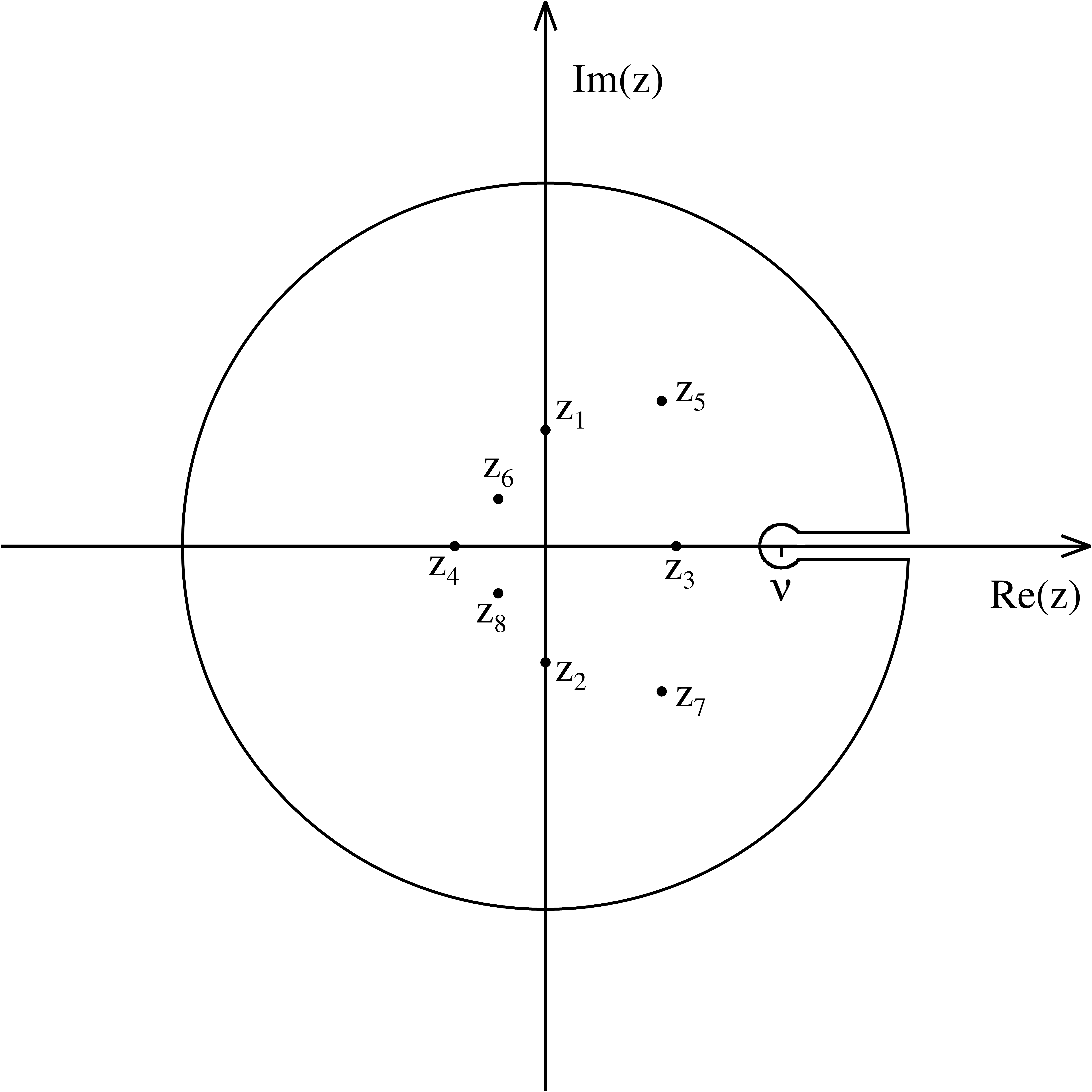
Figure 1: The integration contour with the poles for the function $f_{0}(y)\ln(y-\nu)$ introduced in Section 4.3. The figure corresponds to points $(R,z)$ outside the critical cylinder, i.e. $A>0$ in eq. (19).

For general discussions, it is useful to provide a very elegant commutator-like formula for the quantity $\overline{v^{2}_{\varphi}}-\sigma_{*}^{2}$, related to the study of rotating gaseous baroclinic equilibria (see Barnabè et al. 2006, and references therein):

$$\overline{v_{\varphi}^{2}}-\sigma_{*}^{2}=\dfrac{R}{\rho_{*}}\int_{z}^{\infty}\left(\dfrac{\partial\rho_{*}}{\partial R}\dfrac{\partial\Phi_{\rm t}}{\partial z^{\prime}}-\dfrac{\partial\rho_{*}}{\partial z^{\prime}}\dfrac{\partial\Phi_{\rm t}}{\partial R}\right)dz^{\prime}.$$ (27)

It is not surprising that this relation appears both in Fluidodynamics (Rosseland, 1926; Waxman, 1978) and in Stellar Dynamics (Hunter, 1977), due to the strict relation of the Jeans and fluid equations. We will use eq. (27) for some consideration about the sign of $\overline{v^{2}_{\varphi}}-\sigma_{*}^{2}$ in Section 5, while here we just note how from eq. (27) it follows that for fully spherical models (stars plus dark matter) the commutator vanishes identically, so that, in the Satoh decomposition, such spherical models cannot rotate and are isotropic, a conclusion already reached by using other arguments in Section 3. Finally, in the case of a spherical stellar density, the only non-zero contribution to eq. (27) (and so to rotation in the Satoh decomposition, see eq. 8) can be produced by a non-spherical dark matter halo.

4.3 The contour integral approach

We conclude this Section by noticing that, quite remarkably, the integral in eq. (19) can be expressed in explicit form also by using the Residue Theorem of Complex Analysis. With the change of variable $y=e^{x}$ in eq. (19) we obtain a rational integrand in $y$, which we call $f_{0}(y)$, the integration domain becomes $\nu\leqslant y<\infty$, and $\nu$ is given by eq. (25). It is trivial to prove that the denominator of $f_{0}(y)$ has no real zeros in this range. The numerator of $f_{0}$ has degree 11 and the denominator has degree 16, so that, when considering $y$ a complex variable, the integrand amply satisfies Jordan’s Lemma (e.g., Titchmarsh 1932). The Residue Theorem cannot be applied directly to $f_{0}$ however, as after one circuitation around the origin in the complex plane, the two contributions on the real axis would cancel exactly. This problem can be obviated by applying the Residue Theorem to the suitably modified function $f_{0}(y)\ln(y-\nu)$, where the integration path is schematically given in Fig. 1, so that

$$I=\int_{\nu}^{\infty}f_{0}(y)dy=-\sum{\rm Res}[f_{0}(y)\ln(y-\nu)].$$ (28)

The result holds because the line integrals along the large and small circular paths vanish in the limits of infinite large and small radii, while the $2\pi i$ additive constant, produced by the multivalued factor $\ln(y-\nu)$ along the real axis after the circuitation, leads to the final result. In Fig. 1 we show, for illustrative purposes, the positions of the poles of $f_{0}$ for a generic model, and for $R$ outside the critical cylinder ($A>0$). As the coefficients appearing in $f_{0}$ are real, the poles are either real or they come in complex conjugate pairs; moreover, they are both fixed and movable (i.e., dependent on $R$). Remarkably, all these poles can be expressed as simple algebraic functions, so that the residues can be also calculated explicitly. In fact, there are two fixed quadruple poles at $z_{1,2}=\pm i$, two movable double real poles at $z_{3,4}=(s\pm\sqrt{s^{2}+R^{2}})/R$, and four movable simple poles at $z_{5,6}=(u\pm\sqrt{u^{2}+R^{2}})/R$ and $z_{7,8}=(v\pm\sqrt{v^{2}+R^{2}})/R^{2}$, where $u=s+\sqrt{-A}$ and $v=s-\sqrt{-A}$. These last four poles are real inside the critical cylinder ($A<0$), while they come in two pairs of complex conjugate simple poles outside the critical cylinder; finally on the critical cylinder they merge with the other double real poles $z_{3,4}$, yielding two quadruple real poles. Overall, despite the elegance of this method and the interesting property that the integration can be performed in closed form by using the Residue Theorem, the number of poles, their multiplicity, and their complex nature do not reduce the amount of work needed to obtain the final (real) result when compared with the standard method in Section 4.1.

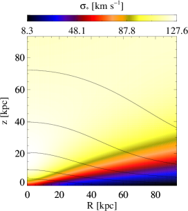
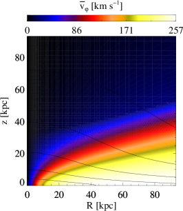
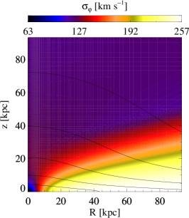
Figure 2: Two-dimensional maps in the meridional plane of the vertical and radial velocity dispersion $\sigma_{*}=\sqrt{\sigma^{2}_{**}+\sigma^{2}_{\rm*h}}$ (left panel), of the ordered azimuthal velocity $\overline{v}_{\varphi}$ in the isotropic case ($k=1$, central panel), and of the azimuthal velocity dispersion $\sigma_{\varphi}$ in the fully velocity dispersion supported case ($k=0$, right panel). The structural parameters of the model are $M_{*}=10^{11}M_{\odot}$, $b=2$ kpc, $s=10$, $v_{\rm h}=250\,\mathrm{km\leavevmode\nobreak\ s}^{-1}$, $R_{\rm h}=5b$, and $q=0.7$. Solid lines represent isodensity contours of the stellar distribution.

5 General properties of the solution

As the Jeans equations of the one component MN model have been already solved (eq. 10 and 11), from the results of Section 4 it follows that a new two-component axisymmetric galaxy model, admitting a fully analytical solution for the Jeans equations for the stellar component is now available. The formulae reported in the text (and in Appendix B) are fully general and they can be easily implemented in numerical codes and in computer algebra systems to explore the behaviour of the kinematical fields of the model in all cases of interest. However, the obtained formulae are sufficiently cumbersome to prevent an immediate reading of their physical content, so that a graphical exploration is useful for a qualitative understanding.

A first illustration of the behaviour of the solutions in the meridional $(R,z)$ plane is given in Fig. 2, where we show the fields $\sigma_{*}$ (left panel), $\overline{v}_{\varphi}$ (central panel) and $\sigma_{\varphi}$ (right panel), for a quite flat MN stellar distribution ($s=10$) of total mass $M_{*}=10^{11}M_{\odot}$, and scale-length $b=2$ kpc, embedded in a maximally flattened DM logarithmic halo with $R_{\rm h}=10$ kpc, $v_{\rm h}=250\,\mathrm{km\leavevmode\nobreak\ s}^{-1}$ and $q=0.7$. For reference, the solid lines show the isodensities of the stellar distribution. As expected, the vertical velocity dispersion $\sigma_{*}$ near the equatorial plane (independent of the specific decomposition of the azimuthal fields) declines for increasing $R$, due to the fact that the MN stellar distribution becomes more and more flat. Of course, in the isotropic case $\sigma_{\varphi}=\sigma_{*}$, and the flattening of the stellar distribution is supported by ordered rotation (central panel). In the fully velocity dispersion supported model (right panel), while $\sigma_{*}$ is the same as in the left panel, $\sigma_{\varphi}$ now supports the flattening, with a field very similar to $\overline{v}_{\varphi}$ of the isotropic rotator. The figures can be compared with the analogous plots in Negri et al. (2014, Fig. 1), which were relative to a rounder stellar MN model ($s=1$), embedded in an Einasto dark matter halo (of exponent $n=4$). Although the models are not exactly the same, the overall structure of the kinematical fields, both in the isotropic ($k=1$) and fully velocity dispersion supported ($k=0$) cases are very similar. The only significant difference is that of an ’hourglass’ structure in $\sigma_{*}$ that can be observed near the centre of the Negri et al. (2014) models, but is missing in Fig. 2. The hourglass shaped distribution is a characteristic of $\sigma_{**}$ for the MN model, and in the present models is absent because of the contribution of the relatively massive Binney halo adopted (at variance with the lighter Einasto halo in Negri et al. 2014): in fact, we checked that, for decreasing values of $v_{\rm h}$, this feature becomes again evident in the present models.

Additional information on the behaviour of the velocity dispersion field as a function of the various parameters of the models can be obtained by inspection of Fig. 3, where we plot the radial trend of $\sigma_{*}^{2}$ in the equatorial plane for a selection of models. In particular, the plots show how the flattening of the stellar distribution and the dark matter halo shape and concentration affect the vertical velocity dispersion of the stellar component. For reference, the black lines represent the contribution to the velocity dispersion due to the one-component MN model in the spherical limit (solid, $s=0$) and for $s=10$ (dashed). Of course, the vertical velocity dispersion field is independent of the amount of anisotropy in the azimuthal motions, so that these plots hold independently of the value of $k$. We can notice a few, obvious features. First, the velocity dispersion of the model without halo is - for each model - lower than the velocity dispersion in presence of the halo. Second, while the velocity dispersion declines at large radii for the MN model, being dominated by the potential monopole term, it flattens to a constant value for models embedded in the logarithmic halo, as expected from the dominance of its quasi-isothermal dark matter profile at large radii. Third, note how a decrease of $R_{\rm h}$ at fixed $q$ and $v_{\rm h}$ leads to an increase of the velocity dispersion, due to the stronger concentration and gravitational field of the halo. We stress again that at the present stage we are not attempting to reproduce any specific object; thus the choice of the three values for $R_{\rm h}$ is just to illustrate the effects of a dark matter halo with a large, moderate, and small scale length, at fixed asymptotic rotational velocity. Of course, “cuspy” haloes are expected to produce dynamical features similar to the ones obtained for $R_{\rm h}=0.5b$.

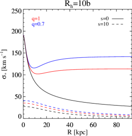
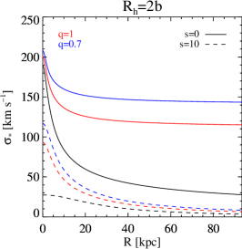
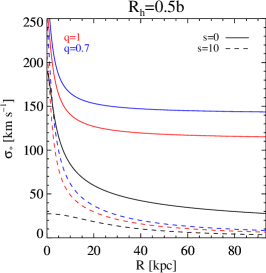
Figure 3: Radial trend of the vertical velocity dispersion $\sigma_{*}$ in the equatorial plane for models with $M_{*}=10^{11}M_{\odot}$, $b=2$ kpc, $v_{\rm h}=250\,\mathrm{km\leavevmode\nobreak\ s}^{-1}$, and different values of $s$, $q$, and $R_{\rm h}$. Solid lines refer to a spherical stellar distribution ($s=0$), while the dashed lines to a flattened MN disc ($s=10$). Red and blue lines correspond to spherical ($q=1$) and maximally flat ($q\simeq 0.7$) equipotentials for the DM halo. For reference, the black curves represent the stellar contribution $\sigma_{**}$. As discussed in the text, the models represented by the blue solid lines cannot be described with the Satoh’s ansatz, and in particular cannot be isotropic.

More interesting are the effects of the halo and stellar flattenings. In particular, for a fixed stellar distribution, an increase of the halo flattening (at fixed $R_{\rm h}$ and $v_{\rm h}$) increases the stellar velocity dispersion at each radius (cf. the pairs of solid or dashed red and blue lines in each panel). The velocity dispersion increase is a consequence of the increase of the vertical gravitational field of the halo, that is more and more equatorially concentrated for decreasing $q$. However, an increase of the flattening of the stellar density distribution (at fixed total stellar mass), for fixed halo, leads to a decrease of the stellar velocity dispersion (cf. solid and dashed lines of given colours). This can appear a curious behaviour, as the same argument above about the intensity of the vertical gravitational field applies, but it is not. In fact, it is true that the vertical gravitational field of the stellar distribution increases for increasing $s$, but the stellar population now has - by construction - a shorter vertical scale-length, so its “temperature” decreases accordingly: the two effects more than compensate, with a resulting net decrease of $\sigma_{*}$. This behaviour is by no means a peculiarity of the present models, and it can be easily proved with simple algebra for the simpler family of oblate Ferrers ellipsoids (Ciotti & Lanzoni, 1997).

Additional properties of the models are given in Fig. 4, where we present, for the same models in the central panel of Fig. 3, the rotational profiles of the stellar component in the equatorial plane, in the isotropic rotator case. In particular, we show the circular velocity, the azimuthal streaming velocity, and the Asymmetric Drift (defined as ${\rm AD}=v_{\rm circ}-\overline{v}_{\varphi}$). The most relevant features are the flattening of $\overline{v}_{\varphi}$ to an asymptotic value that can be easily calculated (see the following discussion). The streaming velocity is almost independent of the flattening of the halo potential, a property reminiscent of $v_{\rm circ}$. Note that we do not show the rotational fields in the case of a spherical density distribution. This is because for a spherical stellar density in a non-spherical halo, the Jeans equations in the isotropic limit admit physical solution only for $q>1$, i.e., for a prolate halo potential. In fact, from eq. (27) it is immediate to show that for a generic spherical stellar density embedded in the logarithmic potential in eq. (3), the quantity $\overline{v_{\varphi}^{2}}-\sigma_{**}^{2}$ is proportional to $q^{2}-1$, and so the Satoh decomposition with $k>0$ cannot be adopted when $q<1$.

A more quantitative analysis of the effects of the model parameters on the dynamical properties of the stellar population is provided by the asymptotic expansion of the solutions. The asymptotic expansion of the dynamical quantities of the one-component MN model is trivial and can be obtained directly from eqs. (10) and (11), hence we do not discuss it here. The asymptotic expansion of the formulae relative to the effects of the dark matter halo on the MN component can also be obtained by working directly on the expressions in Section 4, however it can also be obtained directly from the integral (18). Therefore, the following asymptotic trends (where all lengths are normalized to $b$, and squared velocities are normalized to $GM_{*}/b$) have been obtained with both methods, and have been also verified numerically with our Jeans solver code (Posacki et al., 2013), thus giving an additional and independent check of the analytical integration.

We begin with the behaviour near the origin and we consider only the expansion of $\sigma^{2}_{*}$, being the corresponding formulae for $\overline{v_{\varphi}^{2}}$ obtainable from eq. (7). For a cored DM halo ($R_{\rm h}>0$) $\sigma_{*}^{2}$ and $\overline{v_{\varphi}^{2}}$ are finite at the origin, and their value can be obtained directly from eq. (63) and eq. (27). As the resulting formulae are trivial to obtain and not illuminating, we do not report them here. In the case $R_{\rm h}=0$, a coreless halo, $\sigma_{*}^{2}$ diverges at the centre due to the halo contribution as

$$\sigma_{*}^{2}=-v_{\rm h}^{2}\ln\sqrt{z^{2}+q^{2}R^{2}}+\mathcal{O}(1),$$ (29)

where $\mathcal{O}(1)$ contains the term $\sigma^{2}_{**}(0)$ as obtained from eq. (10). These central trends can be proved also in a simpler way by considering the stellar component of a two-component model that, in the central regions, behaves asymptotically as the MN model. This model is obtained by superimposing to the Binney logarithmic halo the ellipsoidally stratified stellar density

$$\rho_{*}=\frac{\rho_{0*}R_{0*}^{\beta}}{(R_{*}^{2}+R^{2}+z^{2}/p^{2})^{\beta/2}},$$ (30)

where $R_{0*}$ and $R_{*}$ are two scale-lengths, $p$ is the axial ratio of the stellar isodensities, and $\beta>0$ controls the density slope outside the core. For $R_{*}=0$ the density is a pure power-law ellipsoid, while for $R_{*}>0$ the two scale-lengths can be assumed identical. In principle, the constants in eq. (30) could be fixed to match the asymptotic expansion of the MN density distribution near the centre (in particular, $p^{2}=(5+s)/[(1+s)(5+4s+s^{2})]$), but this is not required by the following analysis. The vertical Jeans equation for this two-component model can be integrated for generic positive values of $\beta$ in terms of the Incomplete Euler Beta function (i.e., hypergeometric $\left.{}_{2}F_{1}\right.$ functions, e.g., see eq. 8.391 in Gradshteyn & Ryzhik 2007). Moreover, from Chebyshev (1853) theorem on the integration of binomial differentials, the solution can be expressed in terms of elementary functions for all rational values of $\beta$. Additional elementary cases are obtained for $p=q$ and $R_{\rm h}=R_{*}$ (e.g., see the $\beta=3$ case in Binney & Tremaine 1987). In the present case, it is easy to show that $\sigma^{2}_{*}$ for $\rho_{*}$ in eq. (30), embedded in the potential in eq. (3), diverges exactly like eq. (29) for $R_{\rm h}=0$. Figure 3 illustrates clearly the tendency of $\sigma_{*}$ to diverge at the centre for $R_{\rm h}\to 0$.

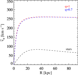
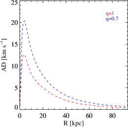
Figure 4: Dashed lines show the radial trend of the rotational properties of the stellar distribution in the equatorial plane for the same models in the central panel of Fig. 3 ($R_{\rm h}=2b$, $s=10$), and two flattenings of the halo potential, $q=1$ (red lines) and $q=0.7$ (blue lines), in the isotropic case. The solid line refers to a spherical stellar distribution ($s=0$). Left panel: the circular velocity $v_{\rm circ}$, a quantity independent of the halo flattening $q$ (see eq. 35). Central panel: the streaming stellar velocity $\overline{v}_{\varphi}$; for reference, the black dashed curve represents the separate contribution of the stellar component. Right panel: the Asymmetric Drift.

We now consider the asymptotic expansion at large distances from the origin. The full expression for $I$ along the $z$ axis ($R=0$) is given in Appendix B.1, and if we let $z$ tend to infinity it follows that

$$\sigma_{*}^{2}=\frac{1}{5}v_{\rm h}^{2}+\mathcal{O}(z^{-1}),$$ (31)

so that the velocity dispersion is dominated by the contribution of the dark matter halo. The treatment of the velocity dispersion in the equatorial plane ($z=0$) for $R\to\infty$ is considerably more complicated. In particular, the asymptotic expansion of the integral (18) can be obtained as a uniformly convergent triple series of integer negative powers of $R$. A careful analysis shows that

$$\sigma_{*}^{2}=\begin{cases}\displaystyle\frac{\xi(q)}{3}v_{\rm h}^{2}+\frac{1}{6R}+\mathcal{O}(R^{-2}),\\[8.61108pt] \displaystyle\left[\frac{1}{q^{2}}+\frac{\xi(q)}{s}\right]\frac{v_{\rm h}^{2}}{R^{2}}+\left[\frac{(s+1)^{2}}{2s}+v_{\rm h}^{2}\tau(q)\right]\frac{1}{R^{3}}+\mathcal{O}(R^{-4}),\end{cases}$$ (32)

where the formulae above hold for $s=0$ and $s>0$, respectively. Note that the formula for the spherical case cannot be obtained as the limit for $s\to 0$ of the case with finite flattening of the stellar component, due to the different behaviour of $\rho_{*}$ in eq. (2) for $a=0$ and $a>0$, respectively. The two functions dependent on the halo flattening (see Fig. 5) are

$$\xi(q)=\frac{q^{2}-4}{(q^{2}-1)^{2}}+\frac{3}{|q^{2}-1|^{5/2}}\begin{cases}\displaystyle\textrm{arctan}\>\sqrt{q^{2}-1},&q>1,\\ \displaystyle\textrm{arctanh}\>\sqrt{1-q^{2}},&q<1,\end{cases}$$ (33)

with $\xi(1)=3/5$, and

$$\begin{split}\tau(q)=&\frac{q^{4}-3q^{2}+17}{(q^{2}-1)^{3}}-\frac{1}{q^{2}}\\ &+\frac{8q^{4}+8q^{2}-1}{q^{3}|q^{2}-1|^{7/2}}\begin{cases}\displaystyle-\textrm{arctanh}\>\frac{\sqrt{q^{2}-1}}{q},&q>1,\\ \displaystyle\textrm{arctan}\>\frac{\sqrt{1-q^{2}}}{q},&q<1,\end{cases}\end{split}$$ (34)

with $\tau(1)=-64/105$. All the trends in Fig. 3 for $R\to\infty$ can be easily verified from the formulae above.

Figure 5: The dimensionless functions $\xi(q)$ and $\tau(q)$ in the asymptotic expansion for $R\to\infty$ of the radial and vertical velocity dispersion in the equatorial plane (eqs. 33 and 34).

In Fig. 4 we showed rotational properties of the stellar component in the equatorial plane, in the isotropic case. Quantitatively, the circular velocity in the equatorial plane is

$$v_{\rm circ}^{2}(R)=\frac{R^{2}}{\left[R^{2}+(s+1)^{2}\right]^{3/2}}+\frac{v_{\rm h}^{2}R^{2}}{R_{\rm h}^{2}+R^{2}},$$ (35)

so that it is independent of the halo flattening $q$; for $R\to\infty$

$$v_{\rm circ}^{2}=v_{\rm h}^{2}+\frac{1}{R}-\frac{R_{\rm h}^{2}v_{\rm h}^{2}}{R^{2}}-\frac{3}{2}\frac{(s+1)^{2}}{R^{3}}+\mathcal{O}\left(R^{-4}\right),$$ (36)

while near the origin

$$v_{\rm circ}^{2}=\begin{cases}\displaystyle v_{\rm h}^{2}+\frac{R^{2}}{(s+1)^{3}}-\frac{3}{2}\frac{R^{4}}{(s+1)^{5}},\\[8.61108pt] \displaystyle\left[\frac{v_{\rm h}^{2}}{R_{\rm h}^{2}}+\frac{1}{(s+1)^{3}}\right]R^{2}-\left[\frac{v_{\rm h}^{2}}{R_{\rm h}^{4}}+\frac{3}{2(s+1)^{5}}\right]R^{4};\end{cases}$$ (37)

the formulae above are correct to $\mathcal{O}\left(R^{6}\right)$, and hold for $R_{\rm h}=0$ and $R_{\rm h}>0$, respectively.

A useful quantity related to the ${\rm AD}$ is given by the difference $v_{\rm circ}^{2}-\overline{v}_{\varphi}^{2}$, that in analytical studies is of easier evaluation than the function $v_{\rm circ}-\overline{v}_{\varphi}$. In fact, for moderate values of the Asymmetric Drift, it follows that ${\rm AD}\simeq(v_{\rm circ}^{2}-\overline{v}_{\varphi}^{2})/(2v_{\rm circ})$ (e.g., Binney & Tremaine, 1987), while for example in the isotropic case

$$v_{\rm circ}^{2}-\overline{v}_{\varphi}^{2}=-\frac{R}{\rho_{*}}\frac{\partial\rho_{*}\sigma^{2}}{\partial R},$$ (38)

as follows from eqs. (7) and (9). Using the asymptotic formula (32), one can show that

$$v_{\rm circ}^{2}-\overline{v}_{\varphi}^{2}=\begin{cases}\displaystyle\frac{5}{3}\xi(q)v_{\rm h}^{2}+\frac{1}{R}+\mathcal{O}(R^{-2}),\\[8.61108pt] \displaystyle\frac{5v_{\rm h}^{2}}{R^{2}}\left[\frac{1}{q^{2}}+\frac{\xi(q)}{s}\right]+\frac{6}{R^{3}}\left[\frac{(s+1)^{2}}{2s}+v_{\rm h}^{2}\tau(q)\right]+\mathcal{O}(R^{-4}),\end{cases}$$ (39)

where the formulae hold for $s=0$ and $s>0$, respectively. Notice that for fixed $s$, the leading order term of the $v_{\rm circ}^{2}-\overline{v}_{\varphi}^{2}$ expansion is a decreasing function of $q$. From eqs. (36) and (39) one obtains the asymptotic formula for $\overline{v}_{\varphi}$ in the equatorial plane for the isotropic rotator, and at the leading order $\overline{v}_{\varphi}\simeq v_{\rm h}$ for all models with $s>0$.

We conclude presenting a qualitative consideration about gas flows in galactic discs, obtained by using one of the results of this paper. In general it is expected (e.g., by chemical evolution studies) that disc galaxies host radial flows in their equatorial regions (e.g., Spitoni et al., 2014, and references therein). These flows influence the chemical and age gradients of stellar populations, with important consequences for galaxy formation and evolution. The problem is how such radial flows are sustained, i.e., what are the mechanisms responsible for the redistribution of the angular momentum of the disc ISM. Proposed mechanisms range from loss of axisymmetry of the gravitational field (e.g., bars, spiral arms, Q-instabilities, etc.), to viscosity (e.g., due to MRI), to gas accretion on the disc of extra-planar material with low specific angular momentum (e.g., Lacey & Fall, 1985; Elmegreen et al., 2014), so that after the mixing the gas falls toward the centre (as the angular momentum of circular orbits, $J_{0}$, increases for increasing $R$ in stable discs). Here we consider an additional, less stochastic mechanism that can lead to radial gas flows, related to internal phenomena, i.e., the coupling between the stellar mass losses of the stars near the equatorial plane and the pre-existing gas. Of course, we are not proposing that this is the only mechanism at work, as accretion of external gas in star-forming disc galaxies is required by pure mass budget arguments. However, it is interesting to consider the possibility that internal phenomena may contribute to radial flows (see also Bilitewski & Schönrich 2012).

We derive the relevant relation between the ${\rm AD}$ and $v_{\rm in}$, the expected inflow velocity of the gas towards the galaxy central regions, restricting to the equatorial plane for the sake of simplicity. Consider some cold gas in the annulus between $R$ and $R+\Delta R$, rotating with $v_{\rm circ}(R)$. Then some other gas, coming from the evolving stellar population (e.g., Ciotti et al. 1991), is added with velocity $\overline{v}_{\varphi}$, the streaming rotational velocity of the stars (e.g., see D’Ercole et al. 2000; Negri et al. 2013 for the hydrodynamical aspects). Because of the asymmetric drift, this new gas has a lower ordered injection velocity than the pre-existing gas, and hence a lower specific angular momentum. The two components mix and the resulting specific angular momentum is the mass-weighted average of both specific angular momenta. The net result will be that the mixed gas will fall inward with some inflow velocity $v_{\rm in}$. Suppose the surface density of the cold gas is given by $\Sigma(R)$, so that its angular momentum in the radial annulus between $R$ and $R+\Delta R$ is given by

$$J_{0}(R)=2\pi R^{2}\Delta R\,\Sigma(R)\,v_{\rm circ}(R).$$ (40)

In a time interval $\delta t$ the evolving stars inject new material at a rate $\dot{\Sigma}(R)$, for an amount of mass

$$\Delta M_{\rm inj}=2\pi R\,\Delta R\,\dot{\Sigma}(R)\,\delta t,$$ (41)

and angular momentum

$$\Delta J_{\rm inj}=2\pi R^{2}\Delta R\,\dot{\Sigma}(R)\,\delta t\,\overline{v}_{\varphi}.$$ (42)

The angular momentum per unit time after the mixing of the new material with the pre-existing one is given by

$$j(R)=\frac{R(\Sigma\,v_{\rm circ}+\dot{\Sigma}\,\delta t\,\overline{v}_{\varphi})}{\Sigma+\dot{\Sigma}\,\delta t}\simeq j_{0}(R)-R\,{\rm AD}\,\delta t\times\frac{\dot{\Sigma}}{\Sigma},$$ (43)

where $j_{0}(R)=Rv_{\rm circ}(R)$ is the specific angular momentum of the cold gas before injection. Since ${\rm AD}>0$, there is a net radial inflow of gas to the radius $R+\delta R$, defined by the condition $j_{0}(R+\delta R)=j(R)$. Assuming a slow evolution (i.e., long characteristic times $\Sigma/\dot{\Sigma}$), and retaining linear order terms in $\delta t$ and $\delta R$, one obtains an expression for the inflow velocity as

$$v_{\rm in}(R)=-\dfrac{R\,{\rm AD}(R)}{j_{0}^{\prime}(R)}\times\dfrac{\dot{\Sigma}(R)}{\Sigma(R)},\qquad\qquad j_{0}^{\prime}=\dfrac{\mathrm{d}j_{0}}{\mathrm{d}R},$$ (44)

(see also eq. 3 in Elmegreen et al. 2014). Of course, a quantitative estimate of $v_{\rm in}$ is beyond the scope of this paper, depending on the detailed temporal and spatial distribution of $\dot{\Sigma}$ and $\Sigma$; however its order of magnitude can be obtained for some typical case. For example, the dashed lines in Fig. 6 represent the radial trend of $R{\rm AD}/j_{0}^{\prime}$ for two specific models. For a typical value of $\dot{\Sigma}/\Sigma=10^{-9}yr^{-1}$, these values lead to a velocity of the order of $v_{\rm in}\simeq 1\,\mathrm{km\leavevmode\nobreak\ s}^{-1}$ around 20 kpc, consistent with the estimates required by chemical evolution models. We notice that the exact term in eq. (44) in the case of a circular velocity described by a power law, $v_{\rm circ}\propto R^{\alpha}$, would predict $R{\rm AD}/j^{\prime}_{0}=R{\rm AD}/[(1+\alpha)v_{\rm circ}]$. This quantity (without the coefficient $1+\alpha$) is shown in Fig. 6 with the dotted lines.

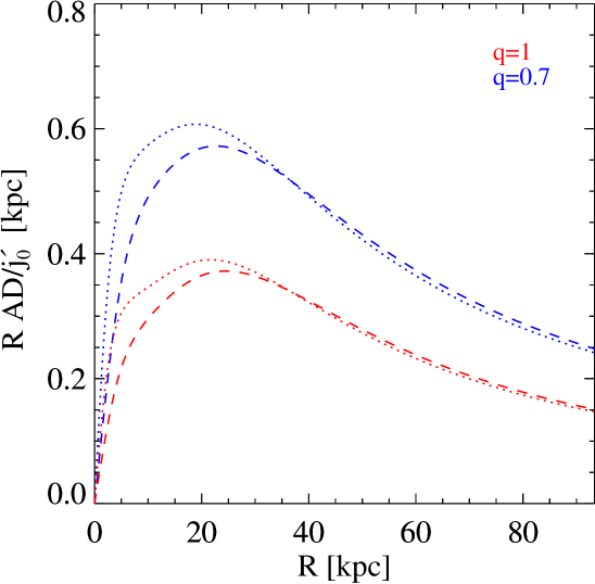
Figure 6: Dashed lines show the radial trend in the equatorial plane of the function $R\times{\rm AD}/j^{\prime}_{0}$, appearing in eq. (44), for the same models in the central panel of Fig. 3 ($R_{\rm h}=2b$, $s=10$), and two flattenings of the halo potential, $q=1$ (red lines) and $q=0.7$ (blue lines), in the isotropic case. The dotted lines show the quantity $R\times{\rm AD}/v_{\rm circ}$, which can be used as a proxy for the true function (see the text below eq. 44 for additional explanations).

6 Discussion and conclusions

In this paper we considered the two-integrals Jeans equations for a new family of two-component galaxy models described by a Miyamoto-Nagai stellar disc embedded in a dark matter Binney logarithmic halo, a cored generalisation of the singular isothermal sphere. We analytically solved these equations and gave the asymptotic behaviour of the quantities involved, both at infinity and near the origin. Moreover, we show that the solution of the Jeans equations for this model can also be obtained with the Residue Theorem.

The obtained formulae have been tested against their numerical solutions, computed with our axisymmetric Jeans solver code (Posacki et al., 2013). Relative errors smaller than $\simeq 10^{-3}$ (or better) are found over the whole computational domains for all the explored combinations of the model parameters. In turns, this is an independent check of our Jeans solver code.

As a simple illustration of our model, we presented the effects of the stellar and dark matter halo flattenings on the vertical velocity dispersion of stars in the equatorial plane. We showed that the velocity dispersion increases with the flattening of the halo, and decreases for increasing flattening of the stellar distribution. As is well known, this is relevant for studies of dark matter densities in the solar neighbourhood (see, e.g., Gilmore et al., 1990; Binney & Tremaine, 1987). We also used the asymmetric drift to obtain estimates for a possible new mechanism that could contribute to sustain radial gas flows in disc galaxies, due to mass loss of stars near the equatorial plane.

The applications just mentioned and explored in a very preliminary way are just a few of many other possible applications, e.g. the study of the circular velocity of gas in the equatorial plane, the building of hydrostatic, barotropic and baroclinic models for hot rotating models (Barnabè et al., 2006), the setup of numerical simulations of gas flows in early-type galaxies with a proper description of thermalisation and stellar motions, etc. Our new model provides a significant addition to the class of known fully analytical axisymmetric models with dark matter haloes.

We notice that recently two papers (Evans & Bowden, 2014; Evans & Williams, 2014) presented new analytical families of axisymmetric dark matter haloes, based on interesting modifications of the Miyamoto-Nagai density-potential pair. In fact, we checked that the Jeans equations for a MN model coupled to these new haloes can also be solved analytically by using the approach here presented.

Appendix A Integration procedure

We summarize the main steps needed to obtain the final formulae in Section 4. The starting point is eq. (19). The special cases $R=0$ ($z$ axis), $A=0$ (critical cylinder), and $s=0$ (spherical stellar density) are treated in Appendix B; the corresponding formulae for these special cases can be obtained as limits of the general solution, but for the sake of simplicity we give them explicitly.

A partial fraction decomposition of the integrand in eq. (19) proves eq. (21):

$$I = \frac{1}{R^{2}}\int_{\textrm{arcsh}\>\lambda}^{\infty}\frac{\alpha_{0}+\alpha_{1}\textrm{sh}\>x+\alpha_{2}\textrm{sh}\>^{2}x+\alpha_{3}\textrm{sh}\>^{3}x}{(1+\textrm{sh}\>^{2}x)^{2}}dx$$ (45)

$$+\frac{1}{R^{2}}\int_{\textrm{arcsh}\>\lambda}^{\infty}\frac{\beta_{0}+\beta_{1}\textrm{sh}\>x}{(R\textrm{sh}\>x-s)^{2}}dx$$

$$+\frac{1}{R^{2}}\int_{\textrm{arcsh}\>\lambda}^{\infty}\frac{\gamma_{0}+\gamma_{1}\textrm{sh}\>x}{A+(R\textrm{sh}\>x-s)^{2}}dx$$

$$= \frac{I_{\alpha}+I_{\beta}+I_{\gamma}}{R^{2}},$$

where $\lambda$ is defined in eq. (20), and the meaning of $I_{\alpha},I_{\beta}$ and $I_{\gamma}$ is obvious.

A.1 The integral $I_{\alpha}$

The partial fraction decomposition coefficients of $I_{\alpha}$ in eq. (45) for $R\neq 0$, $A\neq 0$, and $s\neq 0$ are given by

$$\begin{split}\dfrac{\alpha_{0}\alpha_{d}}{s}=&-17R^{8}-2R^{6}(11s^{2}-12A)\\ &+R^{4}(8s^{4}+19s^{2}A-9A^{2})\\ &+2R^{2}(s^{2}+A)(7s^{4}+A^{2})+s^{2}(s^{2}+A)^{3},\\ \dfrac{\alpha_{1}\alpha_{d}}{R}=&-6R^{8}+R^{6}(14s^{2}+15A)\\ &+2R^{4}(25s^{4}-4s^{2}A-6A^{2})\\ &+R^{2}(34s^{6}+3s^{4}A+4s^{2}A^{2}+3A^{3})\\ &+2s^{2}(2s^{6}+5s^{4}A+4s^{2}A^{2}+A^{3}),\\ \dfrac{\alpha_{2}\alpha_{d}}{s}=&-8R^{8}+R^{6}(2s^{2}+3A)+2R^{4}(13s^{4}+8s^{2}A+3A^{2})\\ &+R^{2}(s^{2}+A)(14s^{4}+9s^{2}A-A^{2})-2s^{2}(s^{2}+A)^{3},\\ \dfrac{\alpha_{3}\alpha_{d}}{R}=&-3R^{8}+2R^{6}(7s^{2}+3A)\\ &+R^{4}(32s^{4}+s^{2}A-3A^{2})+2s^{2}R^{2}(5s^{4}-A^{2})\\ &-s^{2}(5s^{2}+A)(s^{2}+A)^{2},\end{split}$$ (46)

where

$$\alpha_{d}=(R^{2}+s^{2})^{2}[(A+s^{2}-R^{2})^{2}+4R^{2}s^{2}]^{2}.$$ (47)

The integration of the various terms is elementary.

A.2 The integral $I_{\beta}$

The partial fraction decomposition coefficients of $I_{\beta}$ in eq. (45) for $R\neq 0$, $A\neq 0$, and $s\neq 0$ are given by

$$\beta_{0}\beta_{d}=R^{4}s,\qquad\beta_{1}\beta_{d}=R^{3}s^{2},$$ (48)

where

$$\beta_{d}=A(R^{2}+s^{2})^{2}.$$ (49)

Using the standard substitution $y=\textrm{th}\>(x/2)$ we obtain

$$I_{\beta}=-\frac{2\beta_{0}}{s^{2}}\int_{\mu}^{1}\frac{y^{2}-2sy/R-1}{(y^{2}+2Ry/s-1)^{2}}dy,$$ (50)

where $\mu$ is given by eq. (23). It can be easily proved that the two real zeros of the denominator lie outside the integration domain. Elementary integration simplifies to the surprisingly simple expression in eq. (24).

A.3 The integral $I_{\gamma}$

The partial fraction decomposition coefficients of $I_{\gamma}$ in eq. (45) for $R\neq 0$, $A\neq 0$, and $s\neq 0$ are given by

$$\begin{split}\frac{\gamma_{0}\gamma_{d}}{R^{2}s}=&-R^{6}-2R^{4}(s^{2}-3A)-R^{2}(s^{4}-18s^{2}A-3A^{2})\\ &-8A(s^{2}+A)^{2},\\ \frac{\gamma_{1}\gamma_{d}}{R^{3}}=&-R^{4}(s^{2}-3A)-2R^{2}(s^{4}+8s^{2}A+3A^{2})\\ &-(s^{2}-3A)(s^{2}+A)^{2},\end{split}$$ (51)

where

$$\gamma_{d}=A[(A+s^{2}-R^{2})^{2}+4R^{2}s^{2}]^{2}.$$ (52)

At variance with the integrals $I_{\alpha}$ and $I_{\beta}$, the integration procedure now depends on the sign of $A$. Inspection of eq. (45) suggests that an easy factorisation of the denominator of $I_{\gamma}$ could be obtained in the case $A<0$. However, as the same procedure cannot be applied to the case $A>0$ without using complex numbers, we prefer to follow another approach that maximises the similarity of the treatment in the two cases.

The substitution $y=e^{x}$ in the last integral in eq. (45) gives

$$I_{\gamma}=\frac{2\gamma_{1}}{R^{2}}\int_{\nu}^{\infty}\frac{y^{2}+Hy-1}{\Delta(y)}\>dy,$$ (53)

where

$$H=2\frac{\gamma_{0}}{\gamma_{1}},$$ (54)

$$\Delta(y)=y^{4}-\frac{4s}{R}y^{3}+\left(\frac{4A}{R^{2}}+\frac{4s^{2}}{R^{2}}-2\right)y^{2}+\frac{4s}{R}y+1,$$ (55)

and $\nu$ is given by eq. (25).

In principle, we could use the antisymmetry of $\Delta(y)/y^{2}$ (after noticing that $y=0$ is not a zero) to factorise it: it is readily seen that if $y_{1}$ is a zero of $\Delta$, then so is $-1/y_{1}$. This implies that $\Delta(y)/y^{2}$ can be written as a quadratic polynomial in $t=y-1/y$, from which the factorisation is immediate. However, if $A>0$ the two roots of the quadratic polynomial in $t$ are complex conjugates.

In practice this computation is not needed since any quartic polynomial with real coefficients can be factorised into two quadratic polynomials with real coefficients. Without loss of generality, we found it useful to adopt the factorisation

$$\Delta(y)=\left[(y-\Delta_{+})^{2}+\delta_{+}\right]\left[(y-\Delta_{-})^{2}+\delta_{-}\right].$$ (56)

Expansion of eq. (56) and comparison with eq. (55) shows that

$$\Delta_{\pm}=\frac{s}{R}\pm\sqrt{\frac{s^{2}}{R^{2}}+\delta},\qquad\delta_{\pm}=\frac{1-\delta}{\delta}\Delta_{\pm}^{2},\\$$ (57)

where

$$\delta=\frac{\sqrt{(A+s^{2}-R^{2})^{2}+4R^{2}s^{2}}-(A+s^{2}-R^{2})}{2R^{2}}.$$ (58)

Notice that $\delta>0,\Delta_{+}>0,\Delta_{-}<0$. If $A>0$, then $0<\delta<1$ and hence $\delta_{\pm}>0$, making the two quadratic polynomials in eq. (56) irreducible over the reals. If $A<0$, then $\delta>1$ and hence $\delta_{\pm}<0$, consistent with the fact that in this case $\Delta$ can be factorised into four linear factors over the reals.

Now we can proceed in the usual way, by a partial fraction decomposition. The coefficients in

$$\frac{y^{2}+Hy-1}{\Delta(y)}=\frac{\eta_{+}y+\theta_{+}}{(y-\Delta_{+})^{2}+\delta_{+}}+\frac{\eta_{-}y+\theta_{-}}{(y-\Delta_{-})^{2}+\delta_{-}}$$ (59)

are given, after some simplification, by

$$\begin{split}\eta_{\pm}\sigma_{d}=&\pm 2\delta\left(2\delta-\frac{Hs}{R}\right),\\ \theta_{\pm}\sigma_{d}=&2\Delta_{\pm}\left[\frac{s}{R}(\Delta_{+}-\Delta_{-})\pm\delta\Delta_{\pm}(H+2\Delta_{\mp})\right],\end{split}$$ (60)

where

$$\sigma_{d}=4(\Delta_{+}-\Delta_{-})\left(\delta^{2}+\frac{s^{2}}{R^{2}}\right).$$ (61)

Note that a few simple algebraic relations, useful to simplify the final expression of $I_{\gamma}$ in eq. (26), link the constants above:

$$\Delta_{+}^{2}\delta_{-}=\delta_{+}\Delta_{-}^{2}\>,\qquad\frac{\eta_{+}\Delta_{+}+\theta_{+}}{\Delta_{+}}=\frac{\eta_{-}\Delta_{-}+\theta_{-}}{\Delta_{-}}.$$ (62)

Appendix B Special cases

In the following we give the explicit solution of eq. (19) in the special cases $R=0$, $A=0$, $s=0$, when the formulae in Section 4 cannot be used. We recall that $A=q^{2}(R^{2}+R_{\rm h}^{2})-1$.

B.1 Velocity dispersion on the $z$ axis

For $R=0$ (i.e., along the $z$-axis), eq. (18) simplifies considerably, and its integration is elementary:

$$\begin{split}I=&\frac{1}{As^{2}\zeta}+\frac{4s}{(A+s^{2})^{3}}\ln\frac{(\zeta+s)^{2}}{\zeta^{2}+A}-\frac{A+5s^{2}}{s^{2}(A+s^{2})^{2}(\zeta+s)}\\ &-\frac{1}{s(A+s^{2})(\zeta+s)^{2}}\\ &+\frac{3A^{2}-6As^{2}-s^{4}}{A\sqrt{|A|}(A+s^{2})^{3}}\begin{cases}\displaystyle\textrm{arctan}\>\frac{\sqrt{A}}{\zeta},&A>0,\\ \displaystyle\textrm{arctanh}\>\frac{\sqrt{|A|}}{\zeta},&-1\leq A<0.\end{cases}\end{split}$$ (63)

The cases $A=0$ and $A=-s^{2}$ should be treated separately. For $A=0$, i.e., when the critical cylinder coincides with the $z$-axis ($R_{\rm h}=1/q$), then

$$I=\frac{8}{s^{5}}\ln\frac{\zeta+s}{\zeta}+\frac{s^{4}+2s^{3}\zeta-8s^{2}\zeta^{2}-36s\zeta^{3}-24\zeta^{4}}{3s^{4}\zeta^{3}(\zeta+s)^{2}}.$$ (64)

The case $A=-s^{2}$ is possible only for $s<1$, so that $\zeta>s$, and

$$I=\frac{1}{4s^{5}}\ln\frac{\zeta+s}{\zeta-s}-\frac{6s^{3}+10s^{2}\zeta+9s\zeta^{2}+3\zeta^{3}}{6s^{4}\zeta(\zeta+s)^{3}}.$$ (65)

Notice that this solution is always finite, except at the origin ($z=0$, i.e. $\zeta=1$) for $s=1$, so that $A=-1$ on the $z$-axis, which in turn implies $R_{\rm h}=0$, i.e., when the dark matter potential is not cored.

B.2 Velocity dispersion on the critical cylinder

On the critical cylinder $R^{2}=R_{\rm c}^{2}\equiv q^{-2}-R_{\rm h}^{2}$ the parameter $A$ vanishes, and two denominator factors in eq. (19) coincide. Note that, if $qR_{\rm h}>1$, there is no critical cylinder since $A>0$ for every $R$. If $qR_{\rm h}<1$ then $R_{\rm c}$ exists, in particular $R_{\rm c}=1$ for the SIS model. If $qR_{\rm h}=1$ then the critical cylinder coincides with the $z$ axis and the solution for $I$ is given by eq. (64).

The partial fraction decomposition in eq. (45) is no longer valid, instead we have that

$$I=\frac{I_{\alpha}+I_{c}}{R_{\rm c}^{2}},$$ (66)

where $I_{\alpha}$ is as before and $I_{c}$ can, without loss of generality, be written as

$$I_{c}=\sum_{i=1}^{4}\int_{\textrm{arcsh}\>\lambda}^{\infty}\frac{\theta_{i}}{(R_{\rm c}\textrm{sh}\>x-s)^{i}}dx,$$ (67)

where no singularities are contained in the integration domain, and the coefficients $\theta_{i}$ can be found by the usual partial fraction decomposition technique. The substitution $y=e^{x}$ transforms the integrals in rational ones, and in particular

$$\begin{split}\int\frac{dx}{R_{\rm c}\textrm{sh}\>x-s}&=\frac{2}{R_{\rm c}}\int\frac{dy}{y^{2}-2\frac{s}{R_{\rm c}}y-1}\\ &=-\frac{2}{\sqrt{R_{\rm c}^{2}+s^{2}}}\textrm{arctanh}\>\frac{\sqrt{R_{\rm c}^{2}+s^{2}}}{R_{\rm c}-s}.\end{split}$$ (68)

The other integrals for $i=2,3,$ and 4 are most easily obtained by differentiating with respect to $s$ eq. (68). The limits of integration for $y$ are $\nu_{c}$ given by eq. (25) evaluated at $R=R_{\rm c}$, and $\infty$. The final result for $I_{c}$ is

$$\begin{split}I_{c}=&\frac{2R_{\rm c}^{2}(3R_{\rm c}^{4}-24R_{\rm c}^{2}s^{2}+8s^{4})}{(R_{\rm c}^{2}+s^{2})^{9/2}}\textrm{arctanh}\>\frac{\sqrt{R_{\rm c}^{2}+s^{2}}}{R_{\rm c}\nu_{c}-s}\\ &+\frac{2}{3}\frac{R_{\rm c}^{2}s}{(R_{\rm c}^{2}+s^{2})^{4}}\frac{P_{5}(\nu_{c},R_{\rm c})}{(R_{\rm c}\nu_{c}^{2}-2s\nu_{c}-R_{\rm c})^{3}},\end{split}$$ (69)

where

$$\begin{split}P_{5}(\nu,R)=&3R^{2}s(4R^{2}-3s^{2})\nu^{5}\\ &+R(15R^{4}-54R^{2}s^{2}+36s^{4})\nu^{4}\\ &+s(-78R^{4}+100R^{2}s^{2}-32s^{4})\nu^{3}\\ &+6R(-4R^{4}+21R^{2}s^{2}-10s^{4})\nu^{2}\\ &+3R^{2}s(22R^{2}-13s^{2})\nu+R^{3}(13R^{2}-8s^{2}).\end{split}$$ (70)

A careful treatment shows that in the special case where the critical cylinder coincides with the $z$ axis (i.e. $qR_{\rm h}=1$ and $A=R=0$), eq. (66) coincides with eq. (64).

B.3 Spherical stellar density

In the case of a spherical stellar density, i.e., when the MN model reduces to the Plummer sphere, eq. (18) simplifies to

$$I=3\int_{\zeta}^{\infty}\frac{\zeta^{\prime}}{(R^{2}+\zeta^{\prime 2})^{5/2}(A+\zeta^{\prime 2})}d\zeta^{\prime}.$$ (71)

The substitution $u=\sqrt{\zeta^{2}+R^{2}}$ gives a rational integrand, and

$$\begin{split}I=&\frac{1}{(A-R^{2})(R^{2}+\zeta^{2})^{3/2}}-\frac{3}{(A-R^{2})^{2}\sqrt{R^{2}+\zeta^{2}}}\\ &+\frac{3}{|A-R^{2}|^{5/2}}\begin{cases}\displaystyle\textrm{arctan}\>\sqrt{\frac{A-R^{2}}{R^{2}+\zeta^{2}}},&A>R^{2},\\ \displaystyle\textrm{arctanh}\>\sqrt{\frac{R^{2}-A}{R^{2}+\zeta^{2}}},&A<R^{2},\end{cases}\end{split}$$ (72)

while for $A=R^{2}$

$$I=\frac{3}{5(R^{2}+\zeta^{2})^{5/2}}.$$ (73)

References

- Amorisco & Bertin (2010) Amorisco N. C., Bertin G., 2010, A&A, 519, A47
- An & Evans (2006) An J. H., Evans N. W., 2006, ApJ, 642, 752
- Barnabè et al. (2006) Barnabè M., Ciotti L., Fraternali F., Sancisi R., 2006, A&A, 446, 61
- Bertin (2000) Bertin G., 2000, Dynamics of Galaxies
- Bertin & Stiavelli (1984) Bertin G., Stiavelli M., 1984, A&A, 137, 26
- Bilitewski & Schönrich (2012) Bilitewski T., Schönrich R., 2012, MNRAS, 426, 2266
- Binney (1981) Binney J., 1981, MNRAS, 196, 455
- Binney (2014) Binney J., 2014, MNRAS, 440, 787
- Binney & Mamon (1982) Binney J., Mamon G. A., 1982, MNRAS, 200, 361
- Binney & Tremaine (1987) Binney J., Tremaine S., 1987, Galactic dynamics. Princeton Univ. Press, Princeton, NJ
- Carollo et al. (1995) Carollo C. M., de Zeeuw P. T., van der Marel R. P., 1995, MNRAS, 276, 1131
- Chebyshev (1853) Chebyshev P. L., 1853, Journal de mathématiques pures et appliquées, 18, 87–111
- Ciotti (1996) Ciotti L., 1996, ApJ, 471, 68
- Ciotti (1999) Ciotti L., 1999, ApJ, 520, 574
- Ciotti & Bertin (2005) Ciotti L., Bertin G., 2005, A&A, 437, 419
- Ciotti et al. (1991) Ciotti L., D’Ercole A., Pellegrini S., Renzini A., 1991, ApJ, 376, 380
- Ciotti & Giampieri (2007) Ciotti L., Giampieri G., 2007, MNRAS, 376, 1162
- Ciotti & Lanzoni (1997) Ciotti L., Lanzoni B., 1997, A&A, 321, 724
- Ciotti et al. (1996) Ciotti L., Lanzoni B., Renzini A., 1996, MNRAS, 282, 1
- Ciotti & Morganti (2009) Ciotti L., Morganti L., 2009, MNRAS, 393, 179
- Ciotti & Morganti (2010a) Ciotti L., Morganti L., 2010a, MNRAS, 401, 1091
- Ciotti & Morganti (2010b) Ciotti L., Morganti L., 2010b, MNRAS, 408, 1070
- Ciotti et al. (2009) Ciotti L., Morganti L., de Zeeuw P. T., 2009, MNRAS, 393, 491
- Ciotti & Pellegrini (1992) Ciotti L., Pellegrini S., 1992, MNRAS, 255, 561
- Ciotti & Pellegrini (1996) Ciotti L., Pellegrini S., 1996, MNRAS, 279, 240 (CP96)
- Cuddeford (1991) Cuddeford P., 1991, MNRAS, 253, 414
- de Zeeuw et al. (1996) de Zeeuw P. T., Evans N. W., Schwarzschild M., 1996, MNRAS, 280, 903
- Dehnen (1993) Dehnen W., 1993, MNRAS, 265, 250
- Dejonghe (1984) Dejonghe H., 1984, A&A, 133, 225
- Dejonghe (1986) Dejonghe H., 1986, Phys. Rep., 133, 217
- D’Ercole et al. (2000) D’Ercole A., Recchi S., Ciotti L., 2000, ApJ, 533, 799
- Dubinski & Carlberg (1991) Dubinski J., Carlberg R. G., 1991, ApJ, 378, 496
- Eddington (1916) Eddington A. S., 1916, MNRAS, 76, 572
- Elmegreen et al. (2014) Elmegreen B. G., Struck C., Hunter D. A., 2014, ApJ, 796, 110
- Evans (1993) Evans N. W., 1993, MNRAS, 260, 191
- Evans (1994) Evans N. W., 1994, MNRAS, 267, 333
- Evans & Bowden (2014) Evans N. W., Bowden A., 2014, MNRAS, 443, 2
- Evans & de Zeeuw (1994) Evans N. W., de Zeeuw P. T., 1994, MNRAS, 271, 202
- Evans et al. (1990) Evans N. W., de Zeeuw P. T., Lynden-Bell D., 1990, MNRAS, 244, 111
- Evans & Williams (2014) Evans N. W., Williams A. A., 2014, MNRAS, 443, 791
- Gerhard (1991) Gerhard O. E., 1991, MNRAS, 250, 812
- Gilmore et al. (1990) Gilmore G., King I., van der Kruit P. C., 1990, in The Milky Way As Galaxy, SAAS-FEE, Buser R. and King I. eds. (Geneva Observatory)
- Gradshteyn & Ryzhik (2007) Gradshteyn I. S., Ryzhik I. M., 2007, Table of Integrals, Series, and Products, Seventh Edition, Elsevier Academic Press, Jeffrey A., Zwillinger D. e., eds.
- Helmi (2004) Helmi A., 2004, MNRAS, 351, 643
- Hermite (1872) Hermite C., 1872, Annales de Mathématiques, série, 11, 145
- Hernquist (1990) Hernquist L., 1990, ApJ, 356, 359
- Hunter (1977) Hunter C., 1977, AJ, 82, 271
- Jaffe (1983) Jaffe W., 1983, MNRAS, 202, 995
- King (1966) King I. R., 1966, AJ, 71, 64
- Kuzmin (1956) Kuzmin G. G., 1956, AZh, 33, 27
- Lacey & Fall (1985) Lacey C. G., Fall S. M., 1985, ApJ, 290, 154
- Lanzoni & Ciotti (2003) Lanzoni B., Ciotti L., 2003, A&A, 404, 819
- Łokas & Mamon (2001) Łokas E. L., Mamon G. A., 2001, MNRAS, 321, 155
- Merritt (1985) Merritt D., 1985, AJ, 90, 1027
- Michie (1963) Michie R. W., 1963, MNRAS, 126, 499
- Miyamoto & Nagai (1975) Miyamoto M., Nagai R., 1975, PASJ, 27, 533 (MN)
- Nagai & Miyamoto (1976) Nagai R., Miyamoto M., 1976, PASJ, 28, 1
- Navarro et al. (1997) Navarro J. F., Frenk C. S., White S. D. M., 1997, ApJ, 490, 493
- Negri et al. (2014) Negri A., Ciotti L., Pellegrini S., 2014, MNRAS, 439, 823
- Negri et al. (2013) Negri A., Pellegrini S., Ciotti L., 2013, Mem. Soc. Astron. Italiana, 84, 762
- Osipkov (1979) Osipkov L. P., 1979, Pisma v Astronomicheskii Zhurnal, 5, 77
- Pellegrini (2012) Pellegrini S., 2012, in Hot Interstellar Matter in Elliptical Galaxies, ASSL, Vol. 378, pp. 21–54, Kim, D.–W. and Pellegrini, S., eds
- Persic et al. (1996) Persic M., Salucci P., Stel F., 1996, MNRAS, 281, 27
- Plummer (1911) Plummer H. C., 1911, MNRAS, 71, 460
- Posacki et al. (2013) Posacki S., Pellegrini S., Ciotti L., 2013, MNRAS, 433, 2259
- Renzini & Ciotti (1993) Renzini A., Ciotti L., 1993, ApJ, 416, L49
- Rosseland (1926) Rosseland S., 1926, ApJ, 63, 342
- Sarazin & White (1987) Sarazin C. L., White, III R. E., 1987, ApJ, 320, 32
- Satoh (1980) Satoh C., 1980, PASJ, 32, 41
- Siebert et al. (2008) Siebert A. et al., 2008, MNRAS, 391, 793
- Smith et al. (2012) Smith M. C., Whiteoak S. H., Evans N. W., 2012, ApJ, 746, 181
- Spitoni et al. (2014) Spitoni E., Romano D., Matteucci F., Ciotti L., 2014, arXiv:1407.5797
- Titchmarsh (1932) Titchmarsh E. C., 1932, The Theory of Functions, Oxford University Press, 1932, 454 p.
- Toomre (1982) Toomre A., 1982, ApJ, 259, 535
- Tremaine et al. (1994) Tremaine S., Richstone D. O., Byun Y.-I., Dressler A., Faber S. M., Grillmair C., Kormendy J., Lauer T. R., 1994, AJ, 107, 634
- Trenti & Bertin (2005) Trenti M., Bertin G., 2005, A&A, 429, 161
- van der Kruit & de Grijs (1999) van der Kruit P. C., de Grijs R., 1999, A&A, 352, 129
- Van Hese et al. (2009) Van Hese E., Baes M., Dejonghe H., 2009, ApJ, 690, 1280
- Waxman (1978) Waxman A. M., 1978, ApJ, 222, 61
- Williams et al. (2014) Williams A. A., Evans N. W., Bowden A. D., 2014, MNRAS, 442, 1405
- Wilson (1975) Wilson C. P., 1975, AJ, 80, 175
- Zhao (1996) Zhao H., 1996, MNRAS, 278, 488