Orbital and physical parameters of eclipsing binaries from the ASAS catalogue — VIII. The totally-eclipsing double-giant system HD 187669

Abstract

We present the first full orbital and physical analysis of HD 187669, recognized by the All-Sky Automated Survey (ASAS) as the eclipsing binary ASAS J195222-3233.7. We combined multi-band photometry from the ASAS and SuperWASP public archives and 0.41-m PROMPT robotic telescopes with our high-precision radial velocities from the HARPS spectrograph. Two different approaches were used for the analysis: 1) fitting to all data simultaneously with the WD code, and 2) analysing each light curve (with jktebop) and RVs separately and combining the partial results at the end. This system also shows a total primary (deeper) eclipse, lasting for about 6 days. A spectrum obtained during this eclipse was used to perform atmospheric analysis with the moog and sme codes in order to constrain physical parameters of the secondary.

We found that ASAS J195222-3233.7 is a double-lined spectroscopic binary composed of two evolved, late-type giants, with masses of $M_{1}=1.504\pm 0.004$ and $M_{2}=1.505\pm 0.004$ M_⊙, and radii of $R_{1}=11.33\pm 0.28$ and $R_{2}=22.62\pm 0.50$ R_⊙, slightly less metal abundant than the Sun, on a $P=88.39$ d orbit. Its properties are well reproduced by a 2.38 Gyr isochrone, and thanks to the metallicity estimation from the totality spectrum and high precision in masses, it was possible to constrain the age down to 0.1 Gyr. It is the first so evolved galactic eclipsing binary measured with such a good accuracy, and as such is a unique benchmark for studying the late stages of stellar evolution.

1 Introduction

Despite the fortunate configuration of detached eclipsing binaries (DEBs) and many possibilities that it gives us, analysis of these objects still encounters some difficulties. The light curves themselves do not contain enough information about the effective temperatures in the absolute scale, mainly about their ratio. It is sometimes being set on the basis of the colour of the whole system, so combined light of two, sometimes very different stars. Another problem occurs when it comes to calculate the fractional radii (defined as a fraction of the major semi-axis). The information about their sum comes mainly from the width of eclipses, and is somewhat degenerated with the inclination angle, but from the light curves only it is difficult to constrain their ratio. Again, other kinds of data are needed, like spectra, from which one can try to estimate the ratio of fluxes coming from the two components. Both that issues are however much less important in even more fortunate case, when a system shows total eclipses, when light from only one component is seen. The presence of a flat minimum in the light curves already solves the mentioned problems and other kind of observation help to improve the analysis even more.

Such a fortunate situation occurs either when the inclination angle is very close to 90 degrees, or when the two stars have significantly different sizes. The latter usually means that at least one component is evolved. Because of a long-lasting evolution on the main sequence (MS), such evolved systems are much less common than the MS eclipsing binaries. In the recent, very fine summary Torres et al. (2010) point out the lack of red giant systems with accurately measured properties, especially masses and radii. Torres et al. (2010) list only 4 red giants in their sample: AI Phe A, TZ For A, and both components of OGLE-051019.64-685812.3 in the LMC. Since then a small number of systems have been added to the sample, but either containing one giant component (KIC 8410637; Frandsen et al., 2013), or located the Magellanic Clouds (e.g. Pietrzyński et al., 2013; Graczyk et al., 2014), i.e. no galactic double-giant system has been accurately studied. Some interesting cases were analysed (Gałan et al., 2008; Ratajczak et al., 2013) but due to various reasons their parameters are not yet determined precisely enough. Long baseline interferometry was successful in measuring the radii of single red giants directly, but without mass determination. Asteroseismology of solar-type oscillations is another option, and with long-cadence, continuous and precise light curves from CoRoT and Kepler satellites it appears to be a promising method (Kallinger et al., 2009; Bedding et al., 2010), especially if combined with interferometric radius measurements (Baines et al., 2014), but still the precision achieved is lower than for double-lined DEBs, or the differences between parameters obtained from asteroseismology and other methods is significant.

In this paper we present our results of a detailed analysis of a binary system showing a total eclipse, and composed of two cool giant stars – ASAS J195222-3233.7 (HD 187669, CD-32 15534, TYC 7443-867-1; hereafter ASAS-19). Despite being relatively bright – $V\sim 8.9$ mag – this star was recognized as a binary only in the All-Sky Automated Survey (ASAS; Pojmański, 2002) and this is the first detailed study of this interesting target. Time-series photometry is also available in the Public Archive of the Wide-Angle Search for Planets (SuperWASP; Pollacco et al., 2006). Except single-epoch brightness and position measurements, no information is available in other data bases or literature. The only spectral type classification – K0III – comes from Houk (1982).

Two teams were working on this system mostly independently. One group was led by K. Hełminiak (H-group, including MK, MR, PS) and second group by D. Graczyk (G-group, including BP, GP, PK, SV, WG, KS). We used the same data in our analysis and we consulted our partial results as the work progressed. However, overall approach used by each group was different. In the end we combined our results to obtain the final parameters of the system.

2 Observations

Table 1: The PROMPT $V,I$ and ASAS $I$ photometry of ASAS-19. Portion of the table is shown for the reference. The complete table is available in the on-line version of the manuscript.

BJD-2450000	Mag	err	Set
2404.77762	7.567	0.075	AI
2405.80652	7.480	0.071	AI
2406.82007	7.502	0.074	AI
2415.82223	7.494	0.068	AI
2500.62185	7.533	0.074	AI
…

Table 2: RV measurements from disentangling and least-squares spectra fitting (H-group), and RaVeSpAn (G-group), and their residuals (all in km s^-1). Index “1” denotes the hotter star (primary) and “2” the cooler (secondary)

. H-group G-group JD-2450000 $v_{1}$ $(O\!-\!C)_{1}$ $v_{2}$ $(O\!-\!C)_{2}$ $v_{1}$ $(O\!-\!C)_{1}$ $v_{2}$ $(O\!-\!C)_{2}$ 5432.55909 17.346 0.001 -48.742 0.057 16.954 0.014 -49.149 0.075 5467.50740 -47.938 -0.010 16.282 -0.071 -48.140 0.016 15.823 -0.019 5468.49296 -48.725 0.017 17.104 -0.062 -49.002 -0.035 16.582 -0.069 5470.48528 -49.883 0.008 18.228 -0.086 -50.101 0.011 17.705 -0.088 5471.48792 -50.220 -0.007 18.589 -0.046 -50.443 -0.011 18.086 -0.027 5477.66139 -48.393 -0.037 16.770 -0.010 -48.645 -0.075 16.261 0.000 5478.66494 -47.458 -0.013 15.852 -0.019 -47.663 -0.004 15.345 -0.009 5479.50341 -46.618 -0.057 14.973 -0.015 -46.829 -0.054 14.495 0.022 5503.51201 3.903 -0.030 -35.459 -0.041 3.570 -0.056 -35.968 -0.024 5504.50635 5.859 -0.024 -37.428 -0.066 5.546 -0.023 -37.940 -0.055 5721.64681 -29.487 0.073 -1.956 0.031 -29.733 0.140 -2.448 -0.022 5721.75742 -29.746 0.063 -1.700 0.038 -30.050 0.073 -2.150 0.026 5722.65625 -31.774 0.022 0.286 0.039 -32.106 -0.005 -0.199 0.000 5722.77460 -32.030 0.023 0.557 0.054 -32.389 -0.032 0.095 0.037 5811.58372 -32.927 0.029 1.471 0.067 -33.268 -0.006 0.972 0.009 5813.59359 -37.061 -0.010 5.645 0.152 -37.374 -0.032 5.103 0.063 6137.54467 18.418 0.020 -49.839 0.011 17.970 -0.021 -50.208 0.065 6138.52970 18.009 0.002 -49.492 -0.032 17.557 -0.036 -49.896 -0.021 6178.63170 -50.258 -0.038 18.669 0.027 -50.462 -0.018 18.151 0.026 6178.69965 -50.229 0.006 18.687 0.030 -50.472 -0.014 18.183 0.043 6179.54739 -50.351 0.006 18.768 -0.011 -50.556 0.019 18.274 0.018 6179.66679 -50.354 0.010 18.782 -0.004 -50.545 0.037 18.295 0.032 6179.69162 -50.374 -0.009 18.788 0.002 -50.603 -0.020 18.300 0.036 6214.49823 10.895 0.013 -42.425 -0.074 10.573 -0.013 -42.901 -0.007 6240.54579 -2.315 -0.054 -29.200 0.035 -2.614 0.088 -29.579 0.020 6448.94701 -49.097 -0.002 17.506 -0.013 -49.285 0.003 16.964 -0.012

2.1 Photometry

2.1.1 ASAS

The $V$-band photometry of ASAS-19, publicly available from the ASAS Catalogue, spans from November 2000 to December 2009, and contains 406 good quality points (flagged “A” in the original data).

The $I$-band photometry was downloaded from internal ASAS catalogue and spans from May 2000 to June 2009, and contains 247 good points.

2.1.2 SuperWASP

From the SuperWASP public archive we have extracted raw flux measurements of the binary. In order to transform them to magnitudes, we used flux measurements of a nearby, slightly brighter star HD 187742 ($V=8.07$ mag, $SW=8.193$ mag), also classified as K0III (Houk, 1982), which we have previously inspected for variability. We cross-matched the two data sets and removed the obvious outliers from the resulting light curve. Originally, the SuperWASP data spanned from March 2006 to May 2008 (three observing seasons), but we have found that 2007 and 2008 data suffer from large systematic variations, thus we decided to include data only from April and July 2007, when the primary eclipse was recorded, and the observations do not outlay significantly. We ended up with 5554 good data points.

2.1.3 PROMPT

Dedicated photometric observations of ASAS-19 were carried out in $V$ and $I$ bands with the 0.41-m Prompt-4 and Prompt-5 robotic telescopes, located in the Cerro Tololo Inter-American Observatory in Chile. A more detailed description of the observational settings, reduction procedure and calibration to standard photometric system can be found in Hełminiak et al. (2011). The PROMPT observations span about 400 days. In total we secured 1714 and 1400 measurements in $V$ and $I$ bands respectively. The typical exposure times were 5-7 sec for $V$ and 2-3 sec for the $I$ band. Most of the observations were concentrated in the two eclipses, especially in the flat part of the primary one, covered almost completely in both bands between September 20 and 25, 2009.

Table 1 contains PROMPT $V$ and $I$-band, and ASAS $I$-band light curves. The first column is the time stamp BJD-2450000, second and third colums are the measured brightness (in mag) and its formal error. The last column denotes the data set: AI = ASAS $I$, PI = PROMPT $I$, and PV = PROMPT $V$. The complete table is available in the machine-readable form in the electronic version of the manuscript.

2.2 HARPS Spectroscopy

ASAS-19 was observed spectroscopically with the High Accuracy Radial velocity Planet Searcher (HARPS; Mayor et al., 2003), attached to the 3.6-m telescope in La Silla observatory, Chile, between August 2010 and June 2013. A total of 27 spectra were taken in two modes – high efficiency (EGGS) and high RV accuracy.

Fourteen spectra, taken between 2009 and 2013, were obtained in the efficiency EGGS mode. The exposure time was usually between 300 and 600 seconds depending on a seeing conditions at La Silla. We’d like to call special attention to the spectrum from September 10, 2010, taken exactly during the total part of the primary eclipse, when light from only one component was recorded. This spectrum was used for atmospheric analysis, but the radial velocity was not measured.

Thirteen spectra, taken between June 2011 and September 2012, were obtained in the high RV accuracy mode. The exposure time for those observations varied between 780 and 1200 seconds, giving the S/N around 5500Å of 70-120. All spectra were reduced on-site with the available Data Reduction Software (DRS).

3 Analysis

3.1 Radial velocities

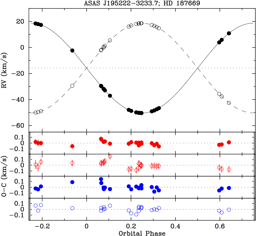
Figure 1: RV measurements and best-fitting orbital solution for ASAS-19. Solid line and filled symbols refer to the primary, and dashed line and open symbols to the secondary component. Differences in RV measurements by two groups are smaller than the size of symbols, and models are practically indistinguishable. Dotted line marks the systemic velocity of the primary. The difference between the two systemic velocities was accounted for. Lower panels depict the residuals for each component and each group (different fits) separately. Phase zero is set to the primary minimum. The resulting $rms$ are 30 and 54 m s^-1 for the primary and secondary respectively from the H-group’s solution (red), and 43 and 42 m s^-1 analogously for the G-group (blue). Colour version of the figure available in the on-line version of the manuscript.

Table 3: Results of the orbital fit to the RVs performed by the H-group.

Parameter	Value	$\pm$
$P$ (d)	88.3891	0.0008
$T_{Q}$ (JD)a	2452069.851	0.043
$K_{1}$ (km s-1)	34.524	0.010
$K_{2}$ (km s-1)	34.461	0.015
$\gamma_{1}$ (km s-1)	-15.846	0.008
$\gamma_{2}-\gamma_{1}$ (km s-1)	0.177	0.015
$a_{12}\sin{i}$ (R⊙)	120.549	0.036
$e$	0.0	(fix)
$q$	1.0018	0.0005
$M_{1}\sin^{3}{i}$ (M⊙)	1.5020	0.0013
$M_{2}\sin^{3}{i}$ (M⊙)	1.5047	0.0011
$rms_{1}$ (m s-1)	30
$rms_{2}$ (m s-1)	54
DOF	43
$\chi^{2}/DOF$	0.9963

^a For a quadrature before the primary eclipse.
Not adopted in further analysis.

3.1.1 H-group

Radial velocities (RVs) were initially calculated with the two-dimensional cross-correlation todcor code (Zucker & Mazeh, 1994), with synthetic spectra taken as templates. These RVs were then used as starting values for the tomographic spectral disentangling and least-squares fitting procedure (Konacki et al., 2010). This procedure uses tomographic methods to produce decomposed spectra of each star, suitable for more precise RV measurements and spectral analysis (after proper scaling). To find the new RVs, the code uses the least-squares method to find shifts of the two spectra in the $\log{\lambda}$ domain, so their sum matches a given observed spectrum.

3.1.2 G-group

Determination of components’ radial velocities was done using RaVeSpAn code (Pilecki et al., 2012) utilizing the Broadening Function formalism (Rucinski, 1992, 1999). We used templates from synthetic library of LTE spectra by Coehlo et al. (2005); the templates were not convolved down to the HARPS resolution. In the beginning we choose templates to match components’ effective temperature, gravity and abundance. However the resulting rms of both radial velocity curves was significantly larger than those from H-group. We decided to investigate the effect. It turned out that using solar metallicity and cooler template (T${}_{\rm eff}\approx 4000$ K) for both components resulted in reducing rms by a factor of 1.5. For more the difference in rms between both stars were reduced to almost zero signifying similar precision of their radial velocity determination. We could expect this because although the secondary rotates two times faster than the primary (producing larger rotational broadening of lines) at the same time it is optically 2.5 times brighter (producing significantly stronger lines in combined spectrum). Both effects should cancel out if there are not other important sources of the scatter (i.e. stellar spots). The resulting radial velocities have slightly larger rms than those derived by tomographic spectral disentangling. Also $\gamma$ difference between components is much smaller – 40 m s^-1– and comparable with individual $rms$ (see further Sections). The overall precision of RV measurements and orbital solutions made by both groups is slightly worse than expected from the spectrograph’s performance. It is probably because of a noticeable rotational broadening of both components and/or stellar activity. Our measurements and their residuals from the WD fit are shown in the Table 2.

3.2 Spectroscopic orbital fit (H-group)

The strategy of the H-group was to obtain partial results with different approaches and working on different data, and combine them into one set later. The orbital fit to the RVs measured by least-squares fitting was done first. The fit was performed with the v2fit code, which is a simple procedure that fits a double-keplerian solution with a Levenberg-Marquardt algorithm. As free parameters we set the two velocity semi-amplitudes $K_{1,2}$, orbital period $P$, centre-of-mass velocity of the primary $\gamma_{1}$, difference between two centre-of-mass velocities $\gamma_{2}-\gamma_{1}$, and a time of phase zero, defined as moment of the periastron passage for eccentric orbits, or a quadrature for circular orbits. Initially we also set free the eccentricity $e$ and argument of the periastron $\omega$, but we have found $e$ to be indifferent from zero.

We have found however that the two components have significantly different values of $\gamma$, with the primary’s (defined here as the hotter star) being blueshifted by $177\pm 15$ m s^-1  – larger than the G-group. Several explanations are possible, but the one we find the most plausible is that it is a systematic introduced by the method used by the H-group, which is optimized for precise measurements of velocity variations, not their absolute values. We also find possible that it was due to stellar spots, which caused time-varying asymmetries in line profiles, which finally led to a template mismatch, or due to different large-scale convective motions in the two stars (Schwarzschild, 1975; Porter & Woodward, 2000). We can exclude the differential gravitational redshift, as it would make the secondary blueshifted.

The measurement errors of the order of single m s^-1 occur to be underestimated, so to get the reduced $\chi^{2}$ close to 1, thus reliable statistical errors of the parameters, we added in quadrature a systematic contribution of of 36 and 52 m s^-1 for the primary and secondary respectively. To account for possible systematics in the final solution, we run 10000 Monte Carlo iterations, perturbing the parameters that were held fixed (i.e. $e$ and $\omega$). We added the MC errors to the statistical ones in quadrature, however they were typically an order of magnitude lower than the statistical ones. All the RV measurements from the tomographic disentangling, together with their residuals from the model RV curve, are shown in the Table 2. Neither of the groups used the spectrum taken in totality for the RV calculations and further modelling. The resulting orbital parameters are presented in Table 3, and the corresponding model RV curves are shown in Figure 1.

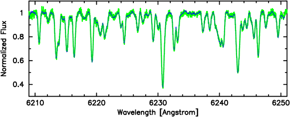
Figure 2: Comparison of the spectrum recorded during the total eclipse (green) with the rescaled secondary’s spectrum from the disentangling (blue). The match is almost perfect, but the disentangled spectrum is of much higher S/N. Colour version of the figure available in the on-line version of the manuscript.

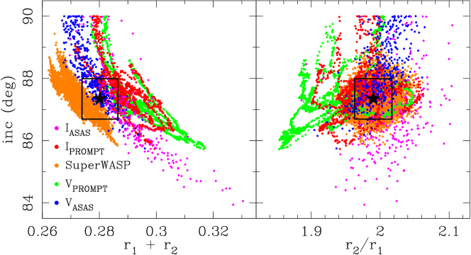
Figure 3: Results of the residual-shifts analysis performed with jktebop on all the data sets separately. Plots present the distribution of consecutive solutions on the $r_{1}+r_{2}$ vs. $i$ (left) and $k=r_{2}/r_{1}$ vs. $i$ (right) panels. Black stars and boxes correspond to the adopted values with their $1\sigma$ uncertainties. Correlation between $r_{1}+r_{2}$ and the inclination is clear, however the inclination itself does not change significantly from set to set. Colour version of the figure available in the on-line version of the manuscript.

3.3 Spectral analysis of the decomposed and total eclipse spectra

3.3.1 moog (G-group)

We disentangled spectra of both components and then we analysed them together with the single spectrum of the secondary component taken at the total primary eclipse. As for disentangling and atmospheric parameters derivation we used the LTE program moog (Sneden, 1973) and follow the prescription given in Graczyk et al. (2014). Details of the method are given in Marino et al. (2008) and the line list in Villanova et al. (2010). The totality spectrum was analysed first, and the temperature $T_{{\rm eff},2}=4360$ K was obtained. The disentangled spectra were scaled using the light ratio determined from solution of radial velocity and light curves, assuming temperature $T_{{\rm eff},2}=4360$ K, by fitting e.g. temperature of the primary $T_{{\rm eff},1}$. The light ratio varied from 2.2490 at 4670 Å, to 2.6712 at 6470 Å. The results are summarized in Tab. 4. Typical errors in $T_{\rm eff}$, $\log{g}$, [$Fe/H$] and $v_{t}$ are 70 K, 0.3, 0.15 dex and 0.2 km s^-1, respectively. Regarding uncertainties parameters derived from the totality spectrum are consistent with those obtained from the disentangled spectrum of the secondary. The small differences on a level of 1$\sigma$ are caused by a little larger depth of absorption lines in disentangled spectrum.

The same procedure of deriving $T_{\rm eff}$ as used here (methodology, and data from HARPS), for Arcturus, a standard star as far as $T_{\rm eff}$ is concern, gives 4290 K (Villanova et al., 2010), which agrees very well with independent measurements (e.g. Ramírez & Allende Prieto, 2011, which gives $T_{\rm eff}=4286$ K). So, in spite of using an LTE approximation, we can recover a reliable $T_{\rm eff}$ for such kind of stars (cold giants at that metallicity) which is essentially free from larger systematic errors.

Table 4: Atmospheric parameters from the moog (G-group)

Spectrum	$T_{\rm eff}$	$\log{g}$	[$Fe/H$]	$v_{t}$
	(K)	(cgs)	(dex)	(km s-1)
primary	4770	2.30	$-0.25$	1.25
secondary	4440	1.60	$-0.22$	1.61
totality	4360	1.57	$-0.44$	1.65
adopteda	4360	1.90b	$-0.30$	1.65

^a For the secondary.
^b From the WD solution.

Table 5: Atmospheric parameters from the sme (H-group)

Spectrum	$T_{\rm eff}$	[$Fe/H$]	$v_{\rm rot}$
	(K)	(dex)	(km s-1)
primary	4610	$-0.24$	6.87
secondary	4310	$-0.21$	13.60
totality	4290	$-0.19$	13.56
adopteda	4300	$-0.20$	13.58

^a For the secondary, from 10 runs.

3.3.2 sme (H-group)

We also analysed the disentangled and total eclipse spectra with the Spectroscopy Made Easy (sme; Valenti & Piskunov, 1996). To ensure that the disentangled spectra are properly scaled, we have used the flux ratios obtained for each echelle order separately, taken from our initial todcor measurements. In the range of the $V$ band they were in a good agreement with the flux ratio obtained from the jktebop solution (next Section). We have also compared the scaled disentangled spectrum of the secondary with the spectrum in totality, and found almost perfect match (Fig. 2).

We run the sme separately on five HARPS orders between 5907 and 6215 Å, with $\log(g)$ being kept fixed to 2.507 and 1.907 for the primary and secondary, respectively – values found in the analysis described in further Sections. For a given component, all runs gave consistent values of $T_{\rm eff}$, [$Fe/H$] and $v_{rot}$, the last one being in agreement with the results expected from the measured radii, assuming spin-orbit alignment and rotational synchronization. As final results we adopted average values of all five runs for the primary, and ten (disentangled + totality) for the secondary, and standard deviations as their uncertainties. We got $T_{\rm eff,1}=4610\pm 50$ K, $[Fe/H]_{1}=-0.24\pm 0.12$ dex, $T_{\rm eff,2}=4300\pm 50$ K, and $[Fe/H]_{2}=-0.20\pm 0.07$ dex. Except $T_{\rm eff,1}$, all values are in a better than 1$\sigma$ agreement with the ones adopted by the G-group (Table 4). However, the final value of $T_{\rm eff,1}$ by the G-group is somewhat lower (Sect. 3.5), and also consistent within 1$\sigma$ with our sme analysis. We summarise our sme results in Table 5. Uncertainties of $v_{\rm rot}$ are 0.3 km s^-1.

Additionally, we estimated the secondary’s effective temperature from the $V-I$ colour vs. line-depth ratio calibrations by Strassmeier & Schordan (2000). We used the totality spectrum and measured 10 ratios of metallic lines from the 6380-6460 Å region, and got the intrinsic secondary’s colour $(V_{2}\!-\!I_{2})_{0}=1.228\pm 0.030$ mag. This corresponds to $T_{\rm eff,2}=4370\pm 80$ K (Worthey & Lee, 2011), and a K2.5-3 III star (Tokunaga, 2000).

3.4 Light curve solution with JKTEBOP (H-group)

Table 6: Results of the jktebop fit to the observed LCs (H-group).

Parameter	$I_{ASAS}$	$V_{ASAS}$	$I_{PROMPT}$	$V_{PROMPT}$	SuperWASP	Adopted
$T_{0}$ (JD-2452000)a	92.118(37)	92.036(47)	92.085(28)	92.095(30)	92.058(17)	92.074(25)
$r_{1}+r_{2}$	0.2929(95)	0.2769(57)	0.2875(73)	0.2931(98)	0.2736(46)	0.2802(63)
$k=r_{2}/r_{1}$	2.014(44)	2.002(23)	1.975(29)	1.933(44)	1.992(22)	1.990(27)
$i$ (deg)	86.5(1.2)	88.0(1.1)	87.52(62)	87.20(79)	87.30(46)	87.34(65)
$r_{1}$	0.0971(40)	0.0923(24)	0.0967(31)	0.0999(49)	0.0914(18)	0.0937(23)b
$r_{2}$	0.1958(62)	0.1847(34)	0.1909(44)	0.1932(54)	0.1821(30)	0.1865(59)b
$(L_{2}/L_{1})_{I}$	2.934(93)	—	2.822(82)	—	—	2.871(87)
$(L_{2}/L_{1})_{V}$	—	2.421(43)	—	2.413(78)	—	2.419(51)
$(L_{2}/L_{1})_{SW}$	—	—	—	—	2.404(27)	2.404(27)
$rms$ (mag)	0.025	0.017	0.017	0.017	0.011

^a Mid-time of the primary eclipse; ^b From the adopted sum and ratio of radii.

One of the codes we used for the light curve (LC) analysis was the version v28 of jktebop (Southworth et al., 2004a, b), which is based on the ebop program (Popper & Etzel, 1981). It is a fast procedure working on one set of photometric data at a time, not allowing for analysis of RV curves. On the basis of spectroscopic data we first found the mass ratio and orbital period, which we included in the LC analysis. We found that the orbital period found directly by jktebop is in agreement with the one from RVs, however leading to significantly worse orbital solution. It is because of a longer time span of spectroscopy with respect to PROMPT and SuperWASP observations, and that ASAS data do not include many points in the eclipses.

For jktebop we used the logarithmic limb darkening (LD) law with coefficients interpolated from the tables of van Hamme (1996) for ASAS and PROMPT. For the SuperWASP data we used tables calculated by the developers of the phoebe code. The gravity darkening coefficients and bolometric albedos were always kept fixed at the values appropriate for stars with convective envelopes ($g=0.32$, $A=0.5$). As mentioned before, no significant eccentricity of the orbit of ASAS-19 was found, nor the third light, thus $e$ and $L_{3}$ were kept fixed to 0. We fitted for the sum of the fractional radii $r_{1}+r_{2}$, their ratio $k$, orbital inclination $i$, moment of the primary minimum $T_{0}$, surface brightness ratios $J$, and brightness scales (out-of-eclipse magnitudes in each filter).

To calculate reliable errors, we run the task 9, which uses the residual-shifts method (Southworth, 2008) to asses the importance of the correlated ‘red’ noise, especially strong in the SuperWASP data (Southworth et al., 2011). We have run several tests to check how the final model varies with various LD coefficients and ephemeris, and we did not notice a strong dependence, but to at least partially account for LD coefficients and ephemeris uncertainties, we let them to be perturbed in the residual-shifts simulations. It is a known fact that orbital inclination is correlated with the radii-related parameters, especially their sum. In Figure 3 we show the results of the jktebop analysis on the $r_{1}+r_{2}$ vs. $i$, and $k=r_{2}/r_{1}$ vs. $i$ diagrams. We see that different data sets give similar values of inclination and $k$, but clearly different areas of the $r_{1}+r_{2}$ vs. $i$ plane are occupied. The most likely reason for this inconsistency is the the activity and the location of spots, probably varying in time, and which was not included in the jktebop analysis. As shown for late-type dwarfs (for example: Różyczka et al., 2009; Windmiller, 2010; Hełminiak et al., 2011), location of spots on different components may lead to variations in resulting radii reaching 2-3 per cent, while the accuracy of our photometry may not be enough to detect the spot-originated brightness variations.

As the resulting parameters we adopted weighted averages of the values found from the five data sets. We mark them in Figure 3, together with the adopted 1$\sigma$ errors. The model LCs are presented in Fig. 4. Looking at the scatter of the PROMPT photometry in both eclipses, we can conclude that more spots reside on the primary (hotter, smaller) component. If so, the $rms$ of the H-group’s RV measurements of both components is more likely enhanced by the rotational broadening, than the activity. If it was activity, we could expect larger $rms$ for the (slower rotating) primary, but we observe the opposite. The resulting values of fractional radii $r_{1,2}$, and the inclination are given in Table 6. The oblateness of both components is below 1%, so the usage of jktebop is justified.

Finally, we have used the jktebop solutions to derive observed $V-I$ colours of both components, and estimate their effective temperatures. Please note, that these simple calculations are possible only for totally-eclipsing systems. For the secondary we have simply used the photometry in the total eclipse and got $1.434(1)$ mag. Taking the intrinsic $(V_{2}\!-\!I_{2})_{0}=1.228(30)$ mag from line depth ratios, we get the value of $E(V\!-\!I)=0.206(30)$ mag, and $E(B\!-\!V)=0.161(23)$, assuming $E(V\!-\!I)=1.28\,E(B\!-\!V)$. From the light curve solutions we got magnitude differences between the components: $V_{2}\!-\!V_{1}=-0.959(23)$ and $I_{2}\!-\!I_{1}=-1.145(32)$ mag. We then get the observed primary’s $V\!-\!I=1.082(39)$ mag, and its intrinsic value of $1.046(39)$ mag. This corresponds to $T_{\rm eff,1}=4710\pm 110$ K, (Worthey & Lee, 2011) and a K0.5 III star (Tokunaga, 2000). Interestingly, both temperatures obtained from the calibrations of Worthey & Lee (2011) – 4710 and 4370 K – are 1.7 per cent larger than those from our sme analysis (4630 and 4300 K).

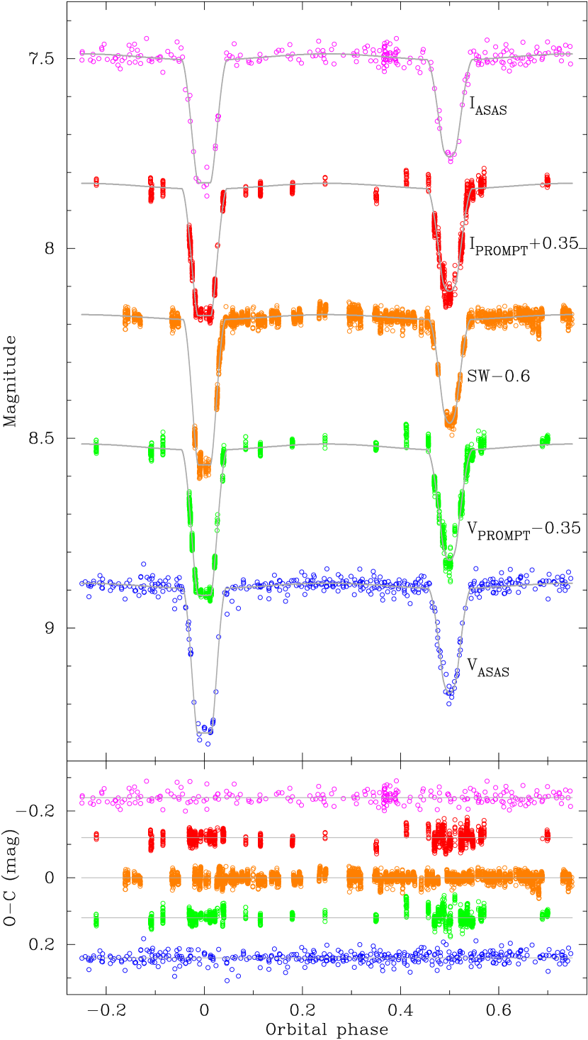
Figure 4: Top: Photometry of ASAS-19 (open circles) and jktebop models (grey lines) for each band. PROMPT and SuperWASP data were shifted for clarity by the indicated values (in mag). Bottom: Residuals of the jktebop models, shifted for clarity. Colour coding and sequence is the same as above. Colour version of the figure available in the on-line version of the manuscript.

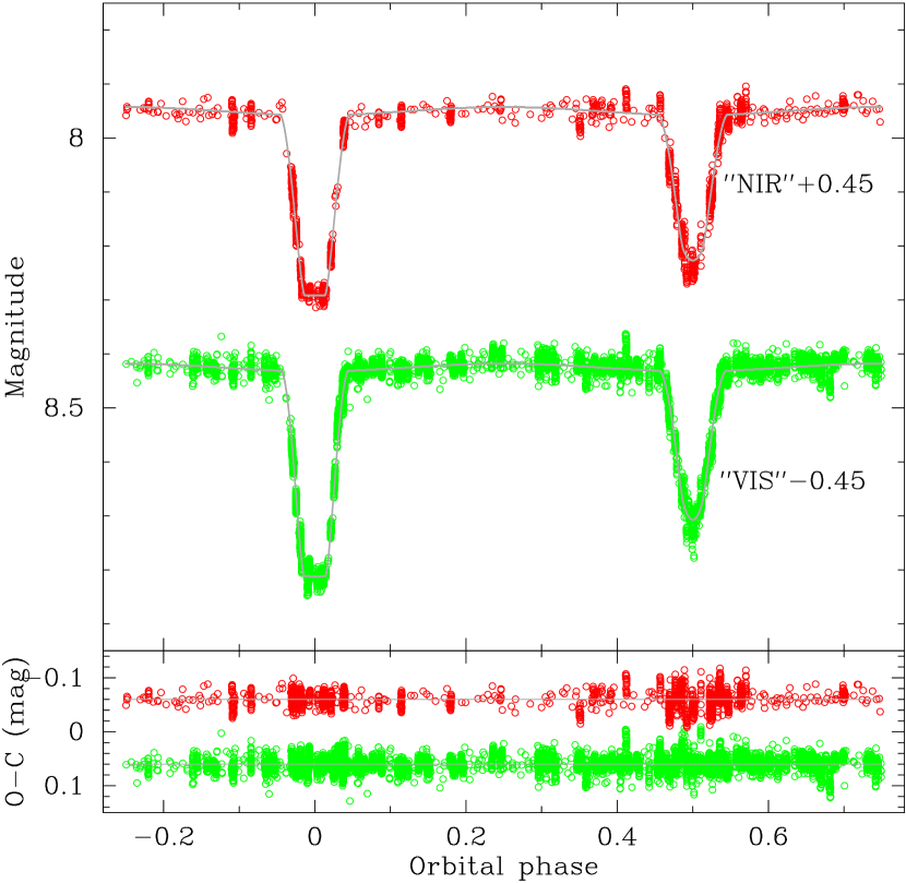
Figure 5: Same as Fig. 4 but for WD models, and combined ”visual” and ”near-infrared” light curves. Colour version of the figure available in the on-line version of the manuscript.

3.5 Simultaneous RV+LC analysis with WD (G-group)

The G-group made the binary model using all data together at the same time. The code used in the analysis was the 2007 version of Wilson-Devinney program (Wilson & Devinney, 1971; Wilson, 1979, 1990; van Hamme & Wilson, 2007). We simultaneously solved all light and radial velocity curves. The light curves were divided into two groups: “visual” – containing all observations in ASAS $V$-band, SuperWASP and PROMPT $V$-band data and “near-infrared” – containing ASAS $I$-band and PROMPT $I$-band data. Within both groups some slight shifts were done to adjust SuperWASP and PROMPT magnitude scales to ASAS magnitudes. The differences in the mean depth and width of the eclipses between different data sets are smaller than systematic effects (night-to-night variations) we noticed in the light curves. In total, the “visual” and “near-infrared” light curves contain 7121 and 1653 points, respectively. We used radial velocities derived from the Broadening Function analysis and we applied a shift of +40 m s^-1 to primary’s velocities to account for its blueshift. The approach to find model solution was essentially similar to method described by Graczyk et al. (2014). The difference was that the primary’s effective temperature was set as free parameter instead of secondary’s one. The reason was that we estimated unique surface temperature of the secondary component from atmospheric analysis of the totality spectrum $T_{2}=4360\pm 80$ K.

We set [$Fe/H$]$=-0.3$ from the atmospheric analysis with moog. The orbital period was kept as a free parameter of a solution. We assumed circular orbit and synchronous rotation of both components. We also checked for the third light, but the fit resulted in negative values, thus we kept it fixed to zero. Logarithmic limb darkening law was used (Klinglesmith & Sobieski, 1970). In total we adjusted 11 parameters of the model. The model LCs are presented in Fig. 5. The resulting parameters are shown in Table 7. We note that our effective temperatures are closer to the values from the Worthey & Lee (2011) calibrations obtained by the H-group, than to their sme results.

Table 7: Results of the WD fit (G-group)

Parameter	Primary	Secondary
$P_{obs}$ (d)	88.3865(27)
$T_{0}$ (JD-2452000)	92.034(97)
$a$ ($R_{\sun}$)	120.51(4)
$q$	1.0004(5)
$i$ (deg)	87.68(15)
$\gamma$ (km s-1)	$-16.19(1)$	$-16.15(1)$
$\Omega^{a}$	11.629(77)	6.323(19)
$r$	0.0941(7)	0.1887(7)
$T_{\rm eff}$ (K)	4687(5)	4360b
$L_{V}$	3.607(7)	8.956(16)
$L_{I}$	3.237(6)	9.307(16)
$K$ (km s-1)	34.458(15)	34.444(15)
RV $rms$ (m s-1)	43	42
$V$-band $rms$ (mag)	0.008
$I$-band $rms$ (mag)	0.016
DOF	8815
$\chi^{2}/$DOF	0.991

^a Dimensionless equipotential of the Roche model.
^b Fixed.

4 Physical parameters

4.1 G-group

Absolute values of parameters were calculated with the WD code, assuming the same astronomical constants as in Table 5 of Graczyk et al. (2012). The distance to the system was derived using di Benedetto (2005) calibration of visual surface brightness vs. $(V\!-\!K)$ colour relation appropriate for giant stars and expressed in Johnson photometric system. We used 2MASS magnitudes from Cutri et al. (2003): $J=6.492$ mag and $K=5.674$ mag and extrapolated components’ light ratio in $J$- and $K$-band from the WD model $l_{21}(J)=3.26$, $l_{21}(K)=3.65$. The 2MASS magnitudes were converted onto Johnson’s system using equations given by Bessell & Brett (1988) and Carpenter (2001). The interstellar reddening was derived from reddening maps (Schlegel et al., 1998) using normalization given by Schlafly & Finkbeiner (2011), assuming a distance to our target (see below) and galactic dust distribution consistent with thin disc model from  Drimmel & Spergel (2001). The resulting $E(B\!-\!V)=0.121\pm 0.016$, where error takes into account uncertainty of total extinction from Schlegel et al. (1998) maps and Milky Way’s thin disc model parameters. The BC’s were calculated from Alonso et al. (1999) calibration for given effective temperature. The derived extinction is almost equal to the extinction estimated by the H-group, which puts confidence in our approach and resulting distance of $614\pm 18$ pc. The distance corresponds to parallax of $1.63\pm 0.05$ mas.

Table 8: Comparison of used approaches. For each method a main advantage and presumable source of systematic errors is given

	G-group			H-group
Analysis stage	Method	Advantages	Systematics	Method	Advantages	Systematics
RVs derivation	RaVeSpAn	direct determination from BF	use of templates	tomography & least-squares fitting	use of disentangled spectra	initial template mismatch
Atmospheric	moog	well calibrated against temperature standards	use of LTE	sme and line depth ratios	line profiles fitting, also blends	use of LTE
Light curves	WD	all light curves simultaneously	fluxes from LTE models; activity	jktebop	fast; red noise accounted for	stellar activity
RV curves	WD	tidal corrections included	relativ. effects not included	v2fit	relativistic eff- ects included	tidal corrections not included
Distance	SB – colour relation	direct, empirical	SB calibration	jktabsdim	average of various methods	calibration of the methods used

Table 9: Physical parameters of the system.

	G-groupa		H-groupb		Adopted
Parameter	Primary	Secondary	Primary	Secondary	Primary	Secondary
Spectrum	K0 IIIc	K2.5 IIIc	K0.5 IIId	K2.5-3 IIId	K0-0.5 III	K2.5 III
$M$ (M☉)	1.501(2)	1.502(2)	1.507(3)	1.509(3)	1.504(4)	1.505(4)
$R$ (R☉)	11.34(9)	22.74(9)	11.31(28)	22.50(71)	11.33(28)	22.62(50)
$\log{g}$ (cgs)	2.505(6)	1.901(3)	2.509(21)	1.913(27)	2.507(20)	1.907(19)
$T_{\rm eff}$ (K)	4687(85)	4360(80)	4610(50)e	4300(50)e	4650(80)	4330(70)
$L$ (L☉)	55.7(4.1)	168(12)	51.9(3.3)	155(12)	53.9(3.9)	161(13)
$M_{\rm bol}$ (mag)	0.39	$-0.81$	0.46	$-0.72$	0.42	$-0.77$
$BC_{V}$ (mag)	$-0.48$	$-0.71$	$-0.44$	$-0.66$	$-0.46$	$-0.69$
$[Fe/H]$	$-0.25(15)$	$-0.30(15)$	$-0.24(12)$	$-0.20(7)$	$-0.25$(10)
Distance (pc)	614(18)		598(18)		606(18)
$E(B\!-\!V)$ (mag)	0.12(2)		0.13(7)		0.13(5)

^a Formal WD fit errors, systematics not always included; ^b Systematics included; ^c According to calibration by Alonso et al. (1999); ^d According to calibration by Tokunaga (2000); ^e From the sme analysis.

4.2 H-group

Absolute values of parameters and their uncertainties were calculated with the jktabsdim code, available together with jktebop, assuming astronomical constants suggested by Harmanec & Prša (2011). This simple code combines the spectroscopic and light curve solutions to derive a set of stellar absolute dimensions, related quantities, and distance. We used photometry from 2MASS in $JHK$ ($J=6.492$, $H=5.674$, $K=5.674$ mag), Tycho (Høg et al., 2000) in $B$ (10.13 mag), and out-of-eclipse combined Johnson’s $V$ magnitude from the jktebop solution (8.866 mag). jktabsdim calculates distances using a number of bolometric corrections for various filters (Bessell et al., 1998; Flower, 1996; Girardi et al., 2002) and surface brightness-$T_{\rm eff}$ relations from Kervella et al. (2004) – 13 in our case. We found $E(B\!-\!V)$ for which the standard deviation of the resulting distance (assumed to be its uncertainty) is the lowest. Outside the given error of $E(B\!-\!V)$, distances differ from each other by more than 1$\sigma$. The result – 0.13(7) mag – is in a good agreement with the one found on the basis of the secondary’s $V\!-\!I$ colours – 0.16(2) mag. Employing this value, and temperatures from calibrations of Worthey & Lee (2011) – 4710 and 4370 K – we get a very similar distance of 604(18) pc.

4.3 Adopted parameters

We combined results from analysis done by our two groups to derive absolute parameters. The comparison of two approaches is presented in Tab. 8, and the final set of physical parameters in Tab. 9. As final values, we adopted straight averages of the two obtained by two groups. To get conservative errors, we took the average of the two uncertainties and added it in quadrature to half of the difference between the two values. When systematics were not included ($R$ and $\log(g)$), we assumed that they are $2\times$ the uncertainty given. All in all, we reached a very good precision in radii (2.5+2.2 per cent), and one of the best estimates of stellar masses in literature (0.27+0.27 per cent). We have also calculated the distance to the system with 3.3 per cent error (total systematic and statistical uncertainty), which translates into 0.05 mas uncertainty in parallax at 606 pc (1.65 mas). Having precisely measured distances on such scales will be important to independently verify the results of the recently launched Gaia mission.

5 Discussion

5.1 Galactic binaries with giant components

In the on-line DEBCat catalogue there are only 17 system listed that have at least one star evolved and larger than 5 R_⊙, and both masses and radii known with accuracy 2 per cent or better. Of these only 3 are galactic systems (others belong to LMC or SMC) and only the primaries are larger than 5 R_⊙. These are V380 Cyg (B1.5 III; Tkachenko et al., 2014), TZ For (Andersen et al., 1991) and KIC 8410637 (Frandsen et al., 2013). A number of other galactic systems have smaller components, although evolved from the main sequence (AI Phe, Andersen et al. 1988, Hełminiak et al. 2009; CF Tau, Lacy et al. 2012; V432 Aur, Siviero et al. 2004), or are much more evolved but measured less precisely (OW Gem, Gałan et al. 2008; $\alpha$ Aur, Torres et al. 2009; ASAS J182510-2435.5 and V1980 Sgr, Ratajczak et al. 2013). This makes ASAS-19 the best measured, evolved galactic binary, and a very unique object, important for studies of late stages of the stellar evolution.

5.2 Age and evolutionary status

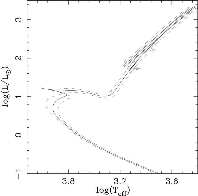
Figure 6: Location of ASAS-19 on the H-R diagram. Black line is the isochrone for $[Fe/H]=-0.25$ and 2.38 Gyr. Two grey dashed lines are are isochrones for $[Fe/H]=-0.15$, 2.55 Gyr (“colder”), and $[Fe/H]=-0.35$, 2.24 Gyr (“hotter”).

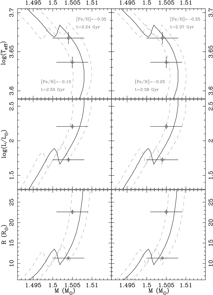
Figure 7: Comparison of our final results with a 2.38 Gyr, $[Fe/H]=-0.25$ isochrone from the PARSEC set (black solid line). Other, marginally-fitting isochrones are plotted in grey (dashed): on the left panels for $(\tau,[Fe/H])=(2.55$ Gyr, $-0.15)$, and $(2.24$ Gyr, $-0.35)$, showing the age uncertainty due to metallicity, and on the right panels for $(\tau,[Fe/H])=(2.37$ Gyr, $-0.25)$, and $(2.39$ Gyr, $-0.25)$, showing the age uncertainty due to mass.

Both stars are currently on the red giant branch, but before the Red Clump (Fig. 6). On this stage of evolution, stars of a similar mass present a wide range of radii, temperatures, luminosities etc., so precise mass and metallicity determination is crucial to constrain their age and exact evolutionary phase. We compared our results from Table 9 with stellar isochrones from the PAdova and tRieste Stellar Evolution Code (PARSEC; Bressan et al., 2012). We used the value of $[Fe/H]=-0.25$, which for this set translates into $Z=0.00855$, $Y=0.2642$. We looked for the age that fits best to our precise and direct mass measurements, and found that ASAS-19 is $2.38^{+0.17}_{-0.14}$ Gyr old. Most of this age uncertainty comes from the [$Fe/H$] determination – for a fixed metal content, the uncertainty coming from the mass determination is only 0.01 Gyr.

In the Figure 7 we show our results on mass vs. temperature, luminosity and radius diagrams, together with various isochrones: the best-fitting (2.38 Gyr, $-0.25$ dex), two for the marginal values of age and metallicity that still reproduce our results within 1$\sigma$ – 2.24 Gyr for $-0.35$, and 2.55 Gyr for $-0.15$ dex (left, also in Figure 6), and two more for fixed metallicity of $-0.25$ dex but the age of 2.37 and 2.39 Gyr (right). One can note, that the 2.38 Gyr, $-0.25$ dex isochrone that fits the mass measurements best, predicts slightly hotter and more luminous stars (Fig. 6). This discrepancy may come from either metallicity or temperatures being a bit underestimated. The 2.38 Gyr, $-0.25$ dex isochrone fits better if temperatures from the calibrations of Worthey & Lee (2011) are used.

5.3 Usefulness of observations during total eclipses

The cases like ASAS-19 allow for independent verification of indirect approaches to determine physical parameters of stars in eclipsing binaries. It shows how the observations performed during a total eclipse are useful for the analysis of DEBs. Especially important was the spectrum taken when only one star was visible. From its analysis we could independently estimate the temperature of one of the components and metallicity of the whole system. Light curves alone do not constrain well the temperature scale, only the ratio of the two $T_{\rm eff}$-s. The common approach to light curve modelling utilizes the observed colour of the whole system, but it works fine only if the components have similar temperature or the total light is dominated by one of them, and only if the observed colour is properly dereddened. In our case we could securely keep one of the $T_{\rm eff}$-s fixed. We could also calculate the observed colours of both stars, one directly from the photometry in the total eclipse, and the other from simple calculations described in Section 3.4. Having the multi-band photometry and the $T_{\rm eff}$ estimation from the spectrum, one can also calculate the $E(B\!-\!V)$ by comparing the colours observed and predicted by colour-temperature calibrations. For nearby systems, where the interstellar extinction is not significant, the observed colours would be enough to calculate the temperature of both components.

We have also used the totality spectrum to estimate the metallicity of the system. This helped us to constrain the age of the binary. The well known age-metallicity degeneration is weaker for red giants than for main sequence stars, but is still present. As we’ve found in Section 5.2, 0.1 dex uncertainty in [$Fe/H$] translates into 0.1 Gyr error in age. For main sequence objects it is at least 10 times more, but it would still be enough to discriminate between stars that have just started their MS evolution, and those that are about to finish it soon.

Metallicity can also be estimated from tomographically disentangled spectra, but the disentangled spectra have to be correctly renormalized in order to account for the companion’s continuum which dilutes the depth of the absorption lines. It is relatively easy for systems showing total eclipses, as from the depth of this eclipse it is straightforward to calculate the contribution of each component, and it also allows us to check if the flux ratio inferred from todcor is correct. It is also possible to verify the results of decomposition by comparing the decomposed and totality spectra, as in Figure 2. As one can see, the disentangled spectra are of higher S/N, however, the approach we used (H-group) requires at least 8 observations in evenly-spread orbital phases. For totally-eclipsing systems, having a single observation during the total eclipse is less time-consuming and can give important results with less effort. We also want to note, that the decomposition itself is easier, as for each observed composite spectrum it is required to know only two parameters: the velocity difference for the component visible in totality and the flux ratio, both of which can be estimated separately or are easy to fit for.

Finally we want to emphasize that a high signal-to-noise spectrum taken during totality can also be a very good template for RV measurements of at least one component, as it obviously matches its $T_{\rm eff}$, $\log{g}$, [$Fe/H$] and turbulence velocities.

References

- Alonso et al. (1999) Alonso A., Arribas S., Martínez-Roger C., 1999, A&ASS, 140, 261
- Andersen et al. (1988) Andersen J., Clausen J. V., Nordström B., Gustaffson G., Vandenberg D. A., 1988, A&A, 196, 128
- Andersen et al. (1991) Andersen J., Clausen J. V., Nordström B., Tomkin J., Mayor M., 1991, A&A, 246, 99
- Baines et al. (2014) Baines E. K., Armstrong J. T., Schmitt H. R., Benson J. A., Zavala R. T., van Belle G. T., 2014, ApJ, 781, 90
- Bedding et al. (2010) Bedding T. R. et al., 2010, ApJ, 713, 176
- Bessell & Brett (1988) Bessell M. S., Brett J. M., 1988, PASP, 100, 1134
- Bessell et al. (1998) Bessell M. S., Castelli F., Plez B., 1998, A&A, 333, 231
- Bressan et al. (2012) Bressan A., Marigo P., Girardi L., Salasnich B., Dal Cero C., Rubele S., Nanni A., 2012, MNRAS, 427, 127
- Carpenter (2001) Carpenter J. M., 2001, AJ, 121, 2851
- Coehlo et al. (2005) Coelho P., Barbuy B., Meléndez J., Schiavon R. P., Castilho B. V., 2005, A&A, 443, 735
- Cutri et al. (2003) Cutri R. M. et al., 2003, VizieR, Online Data Catalogue, 2246, 0
- di Benedetto (2005) di Benedetto G. P., 2005, MNRAS, 357, 174
- Drimmel & Spergel (2001) Drimmel, R. & Spergel, D. N., 2001, ApJ, 556, 181
- Flower (1996) Flower P. J., 1996, ApJ, 469, 355
- Frandsen et al. (2013) Frandsen S. et al., 2013, A&A, 556, A138
- Gałan et al. (2008) Gałan C., Mikołajewski M., Tomov T., Kolev D., Graczyk D., Majcher A., Janowski J. L., Cikała M., 2008, Observatory, 128, 298
- Girardi et al. (2002) Girardi L., Bertelli G., Bressan A., Chiosi C., Groenewegen M. A. T., Marigo P., Salasnich B., Weiss A., 2002, A&A, 391, 195
- Graczyk et al. (2012) Graczyk D. et al., 2012, ApJ, 750, 140
- Graczyk et al. (2014) Graczyk D. et al., 2014, ApJ, 780, 59
- Harmanec & Prša (2011) Harmanec P., Prša A., 2011, PASP, 123, 976
- Hełminiak et al. (2009) Hełminiak K. G., Konacki M., Ratajczak M., Muterspaugh M. W., 2009, MNRAS, 400, 969
- Hełminiak et al. (2011) Hełminiak K. G. et al., 2011, A&A, 527, A14
- Houk (1982) Houk N., 1982, Michigan Catalogue of Two-dimensional Spectral Types for the HD stars. Volume 3. Declinations -40 deg to -26 deg.
- Høg et al. (2000) Høg E. et al., 2000, A&A, 355, L27
- Kallinger et al. (2009) Kallinger T., Weiss W. W., De Ridder J., Hekker S., Barban C., 2009, ASC, 404, 307
- Kervella et al. (2004) Kervella P., Thévenin F., Di Folco E., Ségransan D., 2004, A&A, 426, 297
- Klinglesmith & Sobieski (1970) Klinglesmith D. A., Sobieski S., 1970, AJ, 75, 175
- Konacki et al. (2010) Konacki M., Muterspaugh M. W., Kulkarni S. R., Hełminiak, K. G., 2010, ApJ, 719, 1293
- Lacy et al. (2012) Lacy C. H. S., Torres G., Claret A., 2012, AJ, 144, 167
- Mayor et al. (2003) Mayor M. et al., 2003, The Messenger, 114, 20
- Marino et al. (2008) Marino, A. F., Villanova, S., Piotto, G., et al., 2008, A&A, 490, 62
- Pietrzyński et al. (2013) Pietrzyński G. et al., 2013, Nature, 495, 76
- Pilecki et al. (2012) Pilecki B., Konorski P., Górski M., 2012, From Interacting Binaries to Exoplanets, IAU Symposium, 282, 301
- Pojmański (2002) Pojmański G., 2002, AcA, 52, 397
- Pollacco et al. (2006) Pollacco D. L. et al., 2006, PASP, 118, 1407
- Popper & Etzel (1981) Popper D. M., Etzel P. B., 1981, AJ, 86, 102
- Porter & Woodward (2000) Porter D. H., Woodward P. R., 2000, ApJS, 127, 159
- Ramírez & Allende Prieto (2011) Ramírez, I. & Allende Prieto, C., 2011, ApJ, 743, 135
- Ratajczak et al. (2013) Ratajczak M., Hełminiak K. G., Konacki M., Jordán A., 2013, MNRAS, 433, 2357
- Różyczka et al. (2009) Różyczka M., Kałużny J., Pietrukowicz P., Pych W., Mazur B., Catelán M., Thompson I. B., 2009, AcA, 59, 385
- Rucinski (1992) Rucinski S. M., 1992, AJ, 104, 1968
- Rucinski (1999) Rucinski S. M., 1999, in Hearnshaw J. B., Scarfe C. D., eds, ASP Conf. Ser. Vol. 185, IAU Colloquium 170, Precise Stellar Radial Velocities. Astron. Soc. Pac., San Francisco, p. 82
- Schlafly & Finkbeiner (2011) Schlafly, E. F. & Finkbeiner, D. P., 2011, ApJ, 737, 103
- Schlegel et al. (1998) Schlegel, D. J., Finkbeiner, D. P. & Davis, M., 1998, ApJ, 500, 525
- Schwarzschild (1975) Schwarzschild M., 1975, ApJ, 195, 137
- Siviero et al. (2004) Siviero A., Munari U., Sordo R., Dallaporta S., Marrese P. M., Zwitter T., Milone E. F., 2004, A&A, 417, 1083
- Sneden (1973) Sneden C., 1973, ApJ, 184, 839
- Southworth (2008) Southworth J., 2008, MNRAS, 386, 1644
- Southworth et al. (2004a) Southworth J., Maxted P. F. L., Smalley B., 2004a, MNRAS, 351, 1277
- Southworth et al. (2004b) Southworth J., Zucker S., Maxted P. F. L., Smalley B., 2004b, MNRAS, 355, 986
- Southworth et al. (2011) Southworth J., Pavlovski K., Tamajo E., Smalley B., West R. G., Anderson D. R., 2011, MNRAS, 414, 3740
- Strassmeier & Schordan (2000) Strassmeier K. G., Schordan P., 2000, AN, 321, 277
- Tokunaga (2000) Tokunaga A.T. 2000, in Allen’s Astrophysical Quantities, 4th edition, ed. A.N. Cox, Springer-Verlag (New York), p. 143.
- Tkachenko et al. (2014) Tkachenko A. et al., 2014, MNRAS, 438, 3093
- Torres et al. (2009) Torres G., Claret A., Young P. A., 2009, ApJ, 700, 1349
- Torres et al. (2010) Torres G., Andersen J., Gimenez A., 2010, A&ARv, 18, 67
- Valenti & Piskunov (1996) Valenti J. A., Piskunov N., 1996, A&AS, 118, 595
- van Hamme (1996) van Hamme W., 1996, AJ, 106, 2096
- van Hamme & Wilson (2007) van Hamme W., Wilson R. E., 2007, ApJ, 661, 1129
- Villanova et al. (2010) Villanova, S., Geisler, D., & Piotto, G., 2010, ApJ, 722, 18
- Wilson & Devinney (1971) Wilson R. E., Devinney E. J., 1971, ApJ, 166, 605
- Wilson (1979) Wilson R. E., 1979, ApJ, 234, 1054
- Wilson (1990) Wilson R. E., 1990, ApJ, 356, 613
- Windmiller (2010) Windmiller G., Orosz J. A., Etzel P. B., 2010, ApJ, 712, 1003
- Worthey & Lee (2011) Worthey G., Lee H.-C., 2011, ApJS, 193, 1
- Zucker & Mazeh (1994) Zucker S., Mazeh T., 1994, ApJ, 420, 806